Investigating Robotaxi Crash Severity Using Geographical Random Forest

Abstract

This paper quantitatively investigates the crash severity of Autonomous Vehicles (AVs) with spatially localized machine learning and macroscopic measures of the urban built environment. We address spatial heterogeneity and spatial autocorrelation, while focusing on land use patterns and human behavior. Our Geographical Random Forest (GRF) model, accompanied with a crash severity risk map of San Francisco, presents three findings that are useful for commercial operations of AVs and robotaxis. First, spatially localized machine learning performed better than regular machine learning, when predicting AV crash severity. Bias-variance tradeoff was evident as we adjust the localization weight hyperparameter. Second, land use was the most important built environment measure, compared to intersections, building footprints, public transit stops, and Points Of Interests (POIs). Third, it was predicted that city center areas with greater diversity and commercial activities were more likely to result in low-severity AV crashes, than residential neighborhoods. Residential land use may be associated with higher severity due to human behavior and less restrictive environment. This paper recommends to explicitly consider geographic locations, and to design safety measures specific to residential neighborhoods, when robotaxi operators train their AV systems.

Keywords— Autonomous Vehicles (AVs); Geographical Random Forest (GRF); Built environment; Land use

1 Introduction

Autonomous Vehicles (AVs) and autonomous taxi commonly known as robotaxi are already on the road. AVs have a fundamentally different motion planning paradigm compared to regular vehicles [1, 2], and its technology is anticipated to “revolutionize the way consumers experience mobility [3]”. AVs plan their movement by sensing the environment with various equipments like LiDAR, RADAR, cameras, ultrasonic, and GPS [4, 5, 6]. Integrating information from these sensors remove human factors from the loop and has a solid potential to improve transportation safety [7, 8].

However, safety concerns remain regarding its commercial operations [9, 10, 11]. Also, there were non-negligible numbers of fatal crash incidents that an AV could not avoid. Data from the National Highway Traffic Safety Administration (NHTSA) shows that there were 3566 vehicle crashes with automated driving systems (Level 3 or higher in Table 1) during August 2021 to February 2025. Among that, 318 (9%) crashes resulted in injuries, and 112 (3%) were fatal [12]. As it is projected that well over half of new car sales in the U.S., Europe, and China can be AVs by 2040 [13], number of injuries and fatalities can accordingly increase. In order to mitigate this, understanding the how and why of AV crashes is essential.

Table 1: SAE J3016 Standard for Driving Automation

Level	Description	Responsibility
		Vehicle	Human
0	No Driving Automation	Momentary Assistance	Drive
1	Driver Assistance	Assistance (brakes or gas)	Drive
2	Partial Driving Automation	Assistance (brakes and gas)	Drive
3	Conditional Driving Automation	Drive (if conditions are met)	Standby for takeover
4	High Driving Automation	Drive (in designated areas)	Ride as passenger
5	Full Driving Automation	Drive	Ride as passenger

A substantial amount of research on identifying factors associated to AV crashes have been made. Based on multiple exploratory data analyses, it is shown that crash occurrence is greatly related to pre-crash scenarios such as whether the vehicle was on intersections or whether it was making a turn [14, 15, 16]. Certain physical factors like lighting conditions and road conditions have also been identified to be associated with crash outcome [17, 18]. This is understood to be caused by the microscopic interaction between AV sensors and the physical environment [19, 20]. However, little works have been attempted to examine the macroscopic pattern between AV crashes and the higher level urban systems like the built environment and land use.

The Built Environment (BE) is a comprehensive description of artificial surroundings built to support human activities: living, recreating, and working [21]. Examples include buildings, parks, sidewalks, commercial signage, shopfronts [22], open space, and utilities [23]. There are multiple BE measures relevant to transportation safety: intersections [24] or roadway characteristics [25], street network connectivity [26], population density [27], development density [28], and even the subjective perception of streetscape [29]. Land Use (LU), an overarching concept that illustrates economic and cultural activities practiced within the BE [30], is another major aspect. LU has been utilized in previous non-AV studies either as area partitions [31, 32] or as specific locations [33, 34]. Also, vehicle travel patterns are governed by how people use places [35, 36, 37]. This behavioral aspect cannot be captured by individual physical elements.

Broadening the scope from individual elements to macroscopic patterns of the BE and LU can be particularly useful in AV safety research because AVs are mobile, and their data geographically distributed across multiple neighborhoods. The performance of AV perception systems, thus the data generating mechanism of AV crashes, can differ by location. This prohibits independent and identical distribution of data, and a model obtained from one location may not be able to perform well in another location [38, 39]. A macroscopic perspective opens a way to address this problem by incorporating spatial heterogeneity and spatial autocorrelation. Spatial heterogeneity (or spatial non-stationarity) refers to the variation in parametric relationships across geographic space, while spatial autocorrelation (or spatial dependence) describes the tendency of nearby locations to inherently exhibit similar characteristics [40, 41]. Some recent works have successfully incorporated spatially localized methods to their analyses on regular vehicles [42, 43], but these efforts are yet to be extended to AVs and robotaxis.

This paper contributes to the literature in AV crash analysis from a macroscopic urban systems standpoint. We aim to reveal which BE measures and its corresponding LU behavior is associated with AV safety, and propose a novel spatially localized machine learning framework to predict crash outcomes. The remainder of the paper is structured as follows. First, we present a literature review focusing on how previous AV studies leave gaps regarding macroscopic BE patterns and spatial localization. Then, we organize the data, variables, and methodologies used in this study to predict safety outcome (crash severity) and visualize its risk.

2 Literature Review

Existing works extensively investigated the relationship between transportation safety and urban BE patterns. They attempted to identify BE/LU factors significantly associated with crash outcomes of non-AVs. [44] examined BE, LU, socioeconomic factors, and road infrastructure on cyclist-motorist crashes. This paper found that crash occurrence increase with more commercial LU, and decrease with more recreational and residential LU. Similarly, [45] found that commercial LU, road mileage, and intersection density are related with high occurrence crashes. Utilizing a Geographically Weighted Regression (GWR) model, this paper confirms spatial autocorrelation and heterogeneity in BE-safety relationship. GWR had shown better predictive power than standard regression. A review by [46] emphasized the need for considering spatially localized data generating mechanism. Their paper stated that it is unknown whether (1) specific design are substantively safer or (2) different locations have different relationships. [47] particularly address the Modifiable Areal Unit Problem (MAUP) [48], showing that geographical space partitioning based on traffic density is useful in identifying relevant BE features. Employment density, road density, highway density, LU diversity, and public transit accessibility were associated with higher crash occurrence. [33] used Google Street View images, Points Of Interest (POI) density, and a multi-level machine learning framework. The results indicated that educational POIs and corporate POIs were the greatest contributors to crash frequency. [49] continue to investigate BE/LU factors and found that commercial LU, green areas, and bus stations were associated with greater crash occurrence. [43], via a geographically weighted neural network regressor, showed that intersection density and bus stop density have a greater affect on crash frequency than population density, LU diversity, and destination accessibility. The authors suggested that microscopic traffic interactions are more important then macroscopic BE factors.

These works on general transportation shows that BE and LU are considered as an important factor of transportation safety. Examining both microscopic interactions and macroscopic patterns revealed that high density urban development and commercial activities are less safer for vehicles. The need for such comprehensive analysis remains, especially for crash severity. [50] stated in his paper that “there is a lack of research studies investigating the role of … traffic, non-traffic, physical, built-environment parameters”, regarding crash severity. Regarding research methods, spatial heterogeneity and spatial autocorrelation have been explicitly considered for modeling crash risks. Existing literature suggests the need of a spatially localized model for geographically distributed data like vehicle crashes.

However, existing literature focusing exclusively on AVs are often indifferent to these critical topics. The majority of works have weak consideration of the BE and its geospatial patterns. [14] used AV collision reports from California Department of Motor Vehicles (CA DMV) to visually reconstruct crashes and analyze its maneuvers. They showed that crash occurrence of AVs linearly correlate with cumulative miles traveled. [15] revisit the same data and add satellite imagery to analyze road characteristics. Their model indicated that autonomous driving mode, intersections, curbside parking, rear-end collision, and one-way road types were significantly associated with crash severity. [51] extracted keywords with Natural Language Processing (NLP) and built a machine learning classifier to investigate AV crashes involving Vulnerable Road Users (VRUs). They concluded that crosswalks, intersections, traffic signals, pre-crash maneuvers (turning, slowing down, stopping) were good predictors of VRU-related AV crashes. [52] similarly extracted latent topics with NLP and machine learning. When investigating crash severity, controlling the class imbalance problem was highlighted to ensure classification (recall) power. [53] found that manufacturer, facility type, intersection, pre-crash movement, collision direction, lighting condition and accident year are associated with crash severity. [17] and [18] continue update the literature with CA DMV dataset and conclude that lighting, weather, and road surface conditions are major factors in AV crashes, emphasizing the need of reliable sensors. [16] also update the literature by utilizing CA DMV data from April 2018 to January 2024. They implemented a scenario-based program to analyze AV crashes. [54] analyzed POI data from 4 categories: commercial, residential, office, and traffic. With this, they quantified development intensity around the crash sites (buffer analysis) by calculating POI diversity. The authors concluded that dense developments and LU diversity cause complex environments, in which AVs can malfunction. [55] included more specified variables: metro stops, trees, LU, parks, and schools. They found that rain, mixed-use LU, presence of light rail, and driving at night were associated with higher AV crash severity. [56] gathered a much extensive types of POIs, such as community centers, nightclubs, hospitals, ice cream shops, and parking spaces. Their machine learning model showed that entertainment facilities, places of worship, fountains, and nightclubs were positively associated with AV crash severity.

The literature review above presents three takeaways. First, the majority of AV crash analyses naively focused on microscopic effects of individual elements. They did not sufficiently consider the macroscopic, behavioral patterns of the urban systems found in non-AV research. Research on AV safety should also investigate urban scale BE patterns that can embrace beyond roadway design, pre-crash maneuvers, and POIs. Second, existing AV crash analyses did not incorporate spatial heterogeneity or spatial autocorrelation. In order to effectively close the gap in the literature, there is a need to bring spatially localized methodologies from non-AV studies and apply them to AV studies.

3 Methodology

3.1 Data

We used the CA DMV dataset, which had been utilized in many previous AV crash analyses. We utilized a Large Language Model (LLM) to extract information from California’s Report of Traffic Accident Involving an Autonomous Vehicle (OL 316) documents. We limited our time frame from 2019 to 2024, and our study area to the City and County of San Francisco. The location, severity, and kernel density estimate (KDE) of 496 AV crashes are shown below in Figure 1. More than half of our data were clustered around downtown San Francisco.

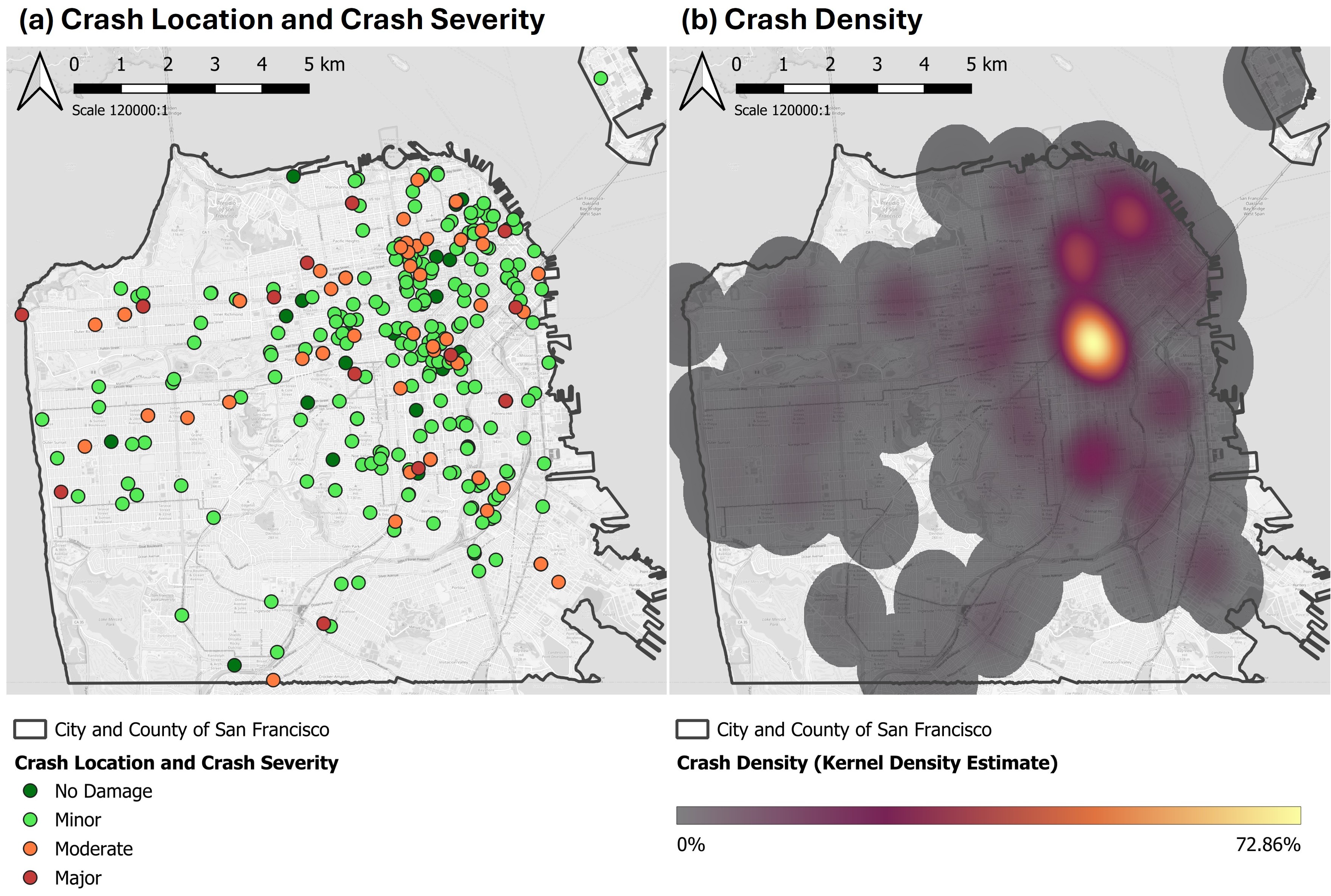
Figure 1: (a) Crash Location and Crash Severity; (b) Crash Density

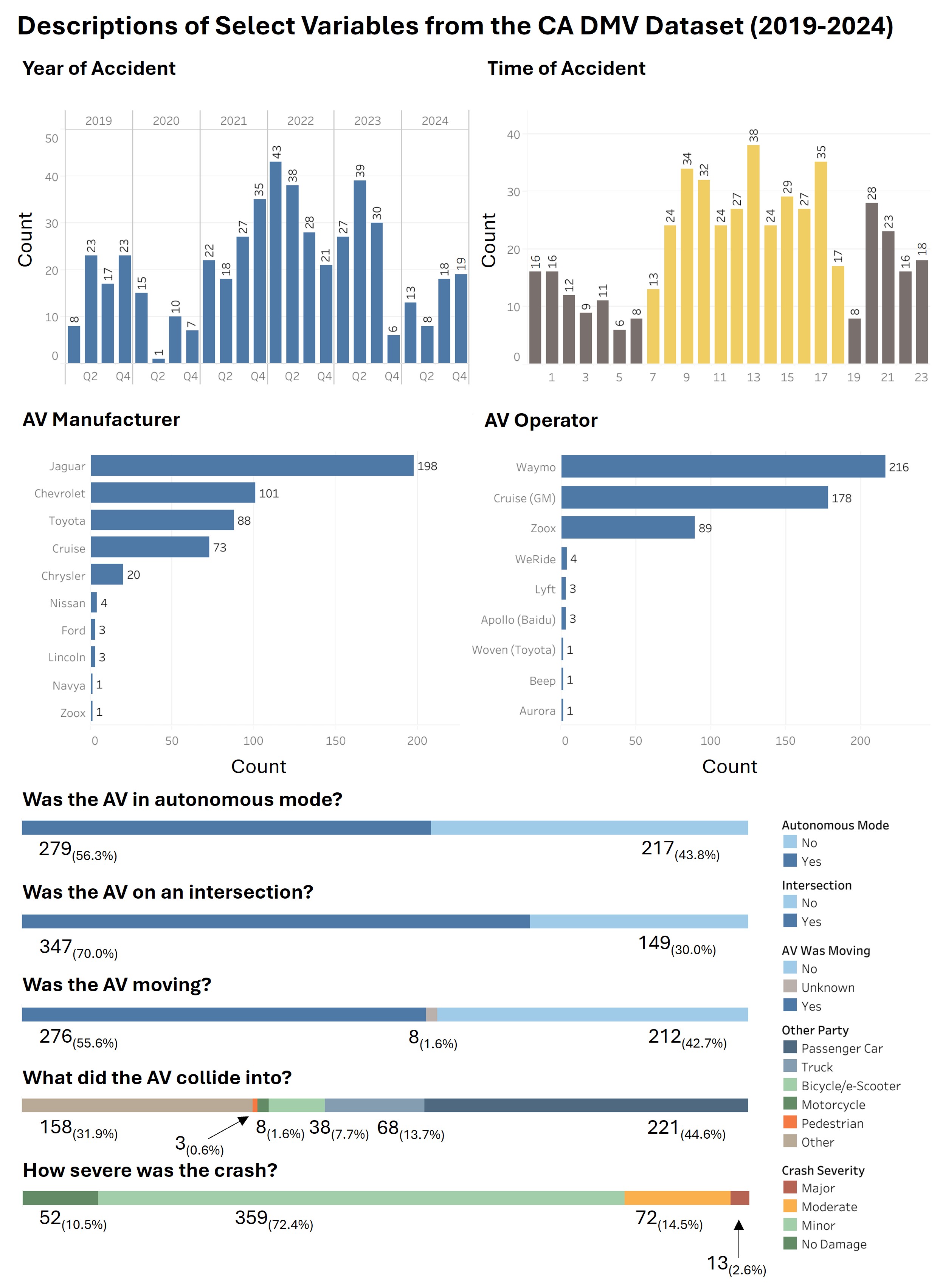
Figure 2: Description of Select Variables from the CA DMV Dataset (2019-2024)

Descriptions of a few select variables are as Figure 2. Accident was most frequent between 2021 and 2023 with a noticeable drop in 2020 Q2 and 2023 Q4. Accidents happened throughout the day except sunrise and sunset. The biggest AV manufacturer was Jaguar, followed by Chevrolet and Toyota. The biggest business operating the AVs was Waymo, followed by Cruise and Zoox. Among 496 accidents, 43.8% happened while autonomous driving was disengaged. 70.0% of accidents happened on an intersection, and 55.6% happened while the AV was moving. The AVs most frequently collided with another passenger car at 44.6%. The crash severity was greatly imbalanced as nearly 83% were Minor or No Damage instances.

3.2 Variables

We select BE variables that can capture the macroscopic, city scale BE patterns and use them to predict AV crash outcomes. We shortlist relevant features as Figure 3. While there is no clear definition on what are microscopic or macroscopic BE features, we implement the ‘5D’ framework. The 5D framework is an extension of the ‘3D’ or ‘4D’ framework [57, 58, 28], and is a well established way to represent high level BE/LU characteristics in transportation studies. In order to quantitatively model the BE-safety relationship, we set BE proxies that comprehensively transcribe the 5Ds while generating tabular data. There are two reasons for setting proxies. First, the five ‘D’s themselves are not individual variables and can be interpreted in multiple interwoven ways [59]. Second, no such index or metric directly representing the 5Ds is available in public data sources.

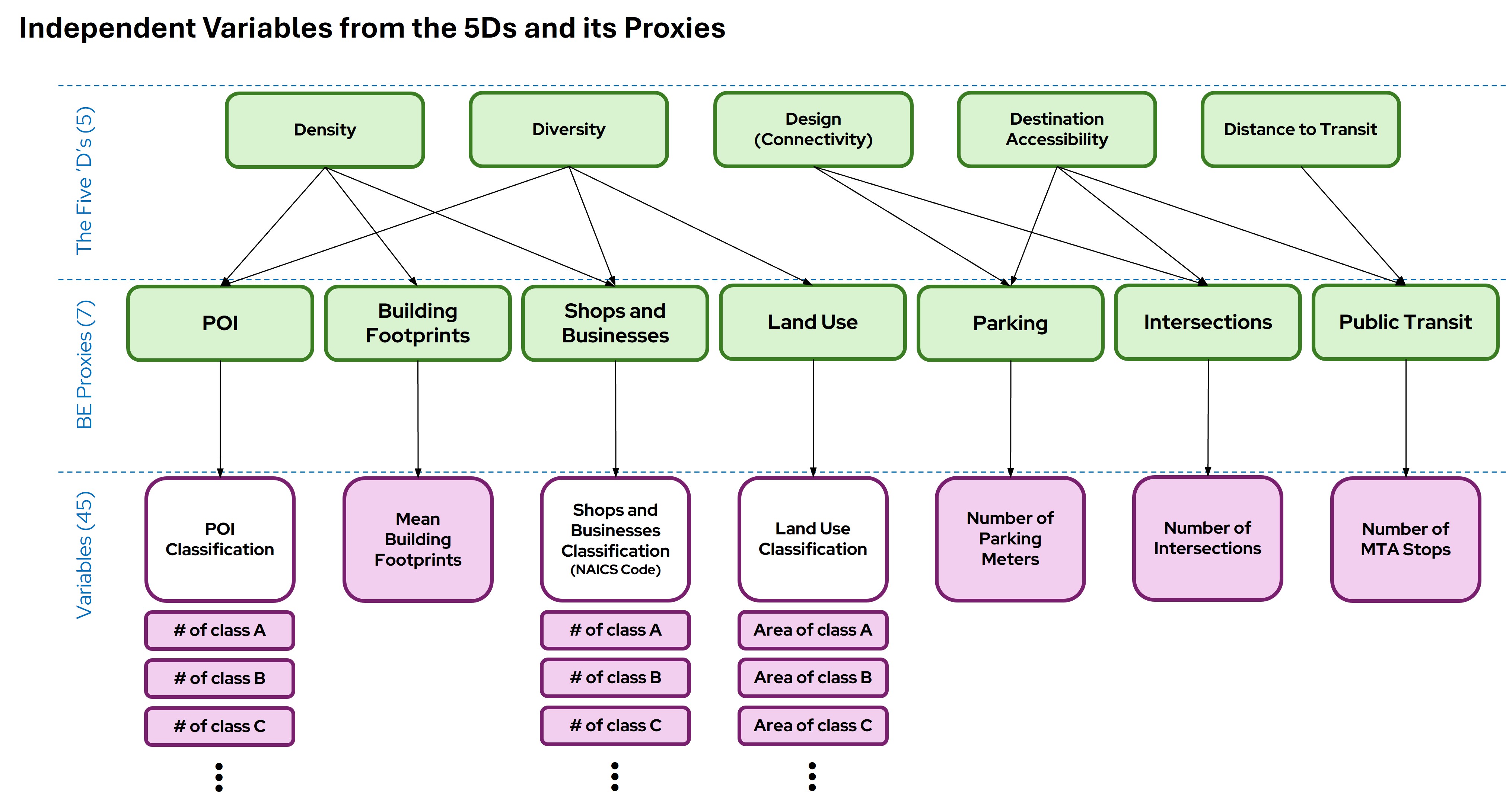
Figure 3: Independent Variables from the 5Ds and its Proxies

The shortlisted 45 independent variables from 7 proxies are as Table 3.2. Descriptions and methodologies for each variable are as follows. (1) POI data has been previously used for building machine learning models that predict crash severity. The categorization of POIs can capture diversity [54] while the types of individual POIs can be an independent variable itself [56]. The number of POIs in proximity to crash sites can indicate density. In this paper, we gathered OpenStreetMap POI data via Overpass Turbo. We used the query amenity=* to extract all available POI features. In total, there were 10 POI categories. All other data are retrieved from San Francisco Open Data Portal, DataSF. (2) Building footprint is the area of land each building occupies. Building footprint is a good indicator of density, which had been investigated in classical studies [28, 60]. It also can differentiate between small-scale and large-scale installations [45]. The dataset we used is individual building geometry built from airborne LiDAR scanning. We calculated the surface area and its centroid of each building via GIS. (3) Shops and businesses are individual locations of registered, tax-paying businesses. The dataset we accessed was last updated at April 13, 2025. Shops and businesses indicate density and diversity of the crash site, along with POIs. Most businesses were tagged with North American Industry Classification System (NAICS) codes, and this enables the classification of businesses. (4) Land use is the current status and nature of how a parcel of land is being used. This is different from zoning regulations that define how land can be used within designated zoning districts. Land use has been used in previous studies [44, 25] and supports the diversity element. DataSF land use dataset (2023) had 12 land use classifications. (5) For parking and public transit, we used the data organized by the San Francisco Municipal Transportation Agency (SFMTA) system, which were available on DataSF. (6) The locations of intersections were obtained by road network data. We extracted all points where two or more roads intersect via GIS.

Table 2: Shortlisted BE Variables

BE Proxy	Variable	Description	Unit	Summary Statistics
				Min	Max	Mean	SD
Points Of	POI Sust	Sustenance (Food & Beverage) POIs	Count	0	393	95.55	72.37
Interests (POI)	POI Edu	Education POIs	Count	0	9	2.46	3.94
	POI Trans	Transportation POIs	Count	0	25	4.89	3.81
	POI Fin	Financial POIs	Count	0	146	10.37	17.46
	POI Health	Healthcare POIs	Count	0	16	2.89	2.59
	POI EAC	Entertainment, Arts, & Culture POIs	Count	0	17	3.32	3.94
	POI Pub	Public Service POIs	Count	0	25	4.89	3.81
	POI Faci	Facilities POIs	Count	0	146	10.37	17.46
	POI Waste	Waste Management POIs	Count	0	63	4.16	6.52
	POI Other	Other POIs	Count	0	53	6.55	8.61
Bldg. Footprint	Mean BFP	Mean Building FootPrint	$\text{ft}^{2}$	94	2078	404.63	344.17
Shops and	Shop Acc	Accommodation	Count	0	144	41.80	25.34
Businesses	Shop Admin	Administrative & Support Service	Count	0	393	25.08	37.67
	Shop AER	Arts, Entertainment, & Recreation	Count	2	162	51.59	29.66
	Shop Cert	Other certain service	Count	0	169	29.27	24.14
	Shop Const	Construction	Count	0	134	35.76	17.64
	Shop Fin	Financial Service	Count	0	1149	36.72	111.66
	Shop Food	Food Service	Count	0	463	111.07	86.28
	Shop Info	Information Service	Count	0	603	34.86	61.61
	Shop Insu	Insurance Service	Count	0	180	4.43	14.26
	Shop Manu	Manufacturing	Count	0	96	11.50	11.68
	Shop PEH	Private Education & Health Serv.	Count	0	430	58.17	68.63
	Shop PST	Professional, Scientific, & Tech. Serv.	Count	0	3143	168.20	283.87
	Shop RERL	Real Estate, Rental & Leasing Serv.	Count	0	1945	183.37	173.00
	Shop Retail	Retail Trade	Count	0	535	91.95	76.29
	Shop Trans	Transportation & Warehousing	Count	0	53	13.62	10.78
	Shop Util	Utilities	Count	0	16	1.38	2.32
	Shop Whole	Wholesale Trade	Count	0	110	15.98	15.38
	Shop Multi	Multiple Classification	Count	0	196	33.52	24.22
	Shop Other	Other unspecified businesses	Count	3	6618	824.21	690.40
Land Use	LU Resident	Residential	$\text{km}^{2}$	0	0.3290	0.1115	0.0859
	LU MixRes	Mixed Use with Residential	$\text{km}^{2}$	0	0.2618	0.0685	0.0397
	LU Mixed	Mixed Use without Residential	$\text{km}^{2}$	0	0.6072	0.0410	0.0512
	LU CIE	Cultural, Institutional, & Education	$\text{km}^{2}$	0	0.3830	0.0194	0.0274
	LU PDR	Production, Distribution, & Repair	$\text{km}^{2}$	0	0.0105	0.0080	0.0119
	LU Medi	Medical	$\text{km}^{2}$	0	0.0487	0.0029	0.0067
	LU Visit	Hotels & Motels	$\text{km}^{2}$	0	0.0488	0.0027	0.0069
	LU MIPS	Mgmt., Info., & Professional Serv.	$\text{km}^{2}$	0	0.3219	0.0349	0.0442
	LU RetailEnt	Retail & Entertainment	$\text{km}^{2}$	0	0.1098	0.0206	0.0228
	LU Openspace	Open Space	$\text{km}^{2}$	0	10.9373	0.3290	1.4143
	LU Vacant	Vacant or undeveloped lots	$\text{km}^{2}$	0	2.8961	0.0648	0.1412
	LU Other	Other unspecified or unknown LU	$\text{km}^{2}$	0	0.2398	0.0038	0.0243
Parking	Parking Meters	SFMTA Parking Meters	Count	0	1222	396.23	340.32
Intersection	Intersections	Intersection of two or more roads	Count	2	91	34.80	16.18
Public Transit	MTA Stops	SFMTA Public Transit Stops	Count	0	35	13.33	7.90

3.3 Quantifying AV Crash Severity Risk

We implemented a machine learning model to quantify AV crash severity risk at a given location. An overview of the pipeline is as Figure 4. As the first step, we conducted a buffer analysis to acquire a tabular data for each shortlisted BE variables. Then, we performed feature selection for our machine learning model with a set a rules.

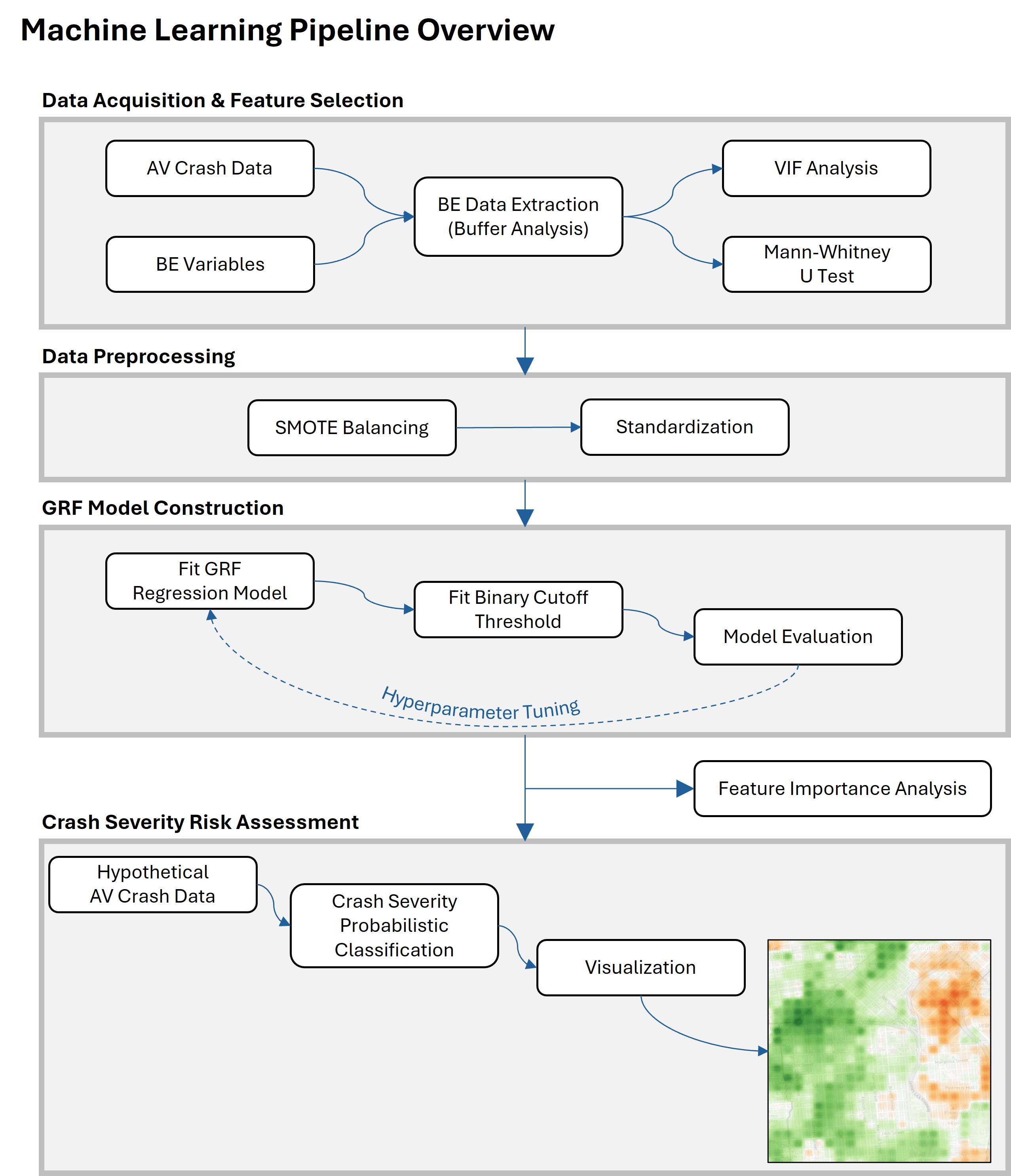
Figure 4: Machine Learning Pipeline Overview

For our buffer analysis, we chose the size of the buffer as the following. According to [5] who collected specifications of multiple AV sensors, the max perception range of AV LiDARs ranged from 30 meters to 245 meters. Since we are interested in the macroscopic BE/LU beyond the AVs’ physical interaction, our size of buffer had to be bigger than this. According to [61] who tried different buffer sizes for machine learning, a buffer of 600 meters showed best results in predicting metro ridership with BE. Since we are interested in road vehicles and their data points are much granular, our size of buffer had to be smaller than this. A common buffer size in urban planning is Perry’s Neighborhood Unit of $\frac{1}{4}$ miles or 400 meters [62, 63]. This value is between 245 and 600 meters. It also have been used in many previous transportation studies [64, 65, 66]. As a result, we have chosen our buffer size as 400 meters.

Feature selection was performed via Mann-Whitney $U$ tests (MWU) and Variance Inflation Factor (VIF) analysis to reduce dimensionality while retaining useful features. MWU is a robust, non-parametric (rank-ordered) counterpart to the $t$-test and is used to determine whether two independent samples come from the same distribution or not [67]. A $t$-test was inappropriate since it requires approximately Gaussian distributions, homogeneous variance, and similar sample sizes between the (crash severity) categories [68]. The resulting $p$-values from MWU are the probability of the two samples coming from two indistinguishable distributions. In our study, we reassigned the crash severity into High and Low to perform a pairwise MWU. VIF detects multicollinearity of each variables. It measures how much it inflates a linear model’s regression coefficients by fitting one variable with all other variables. Excessively high VIF can make the model redundantly complex and less interpretable [69]. A variable with VIF $>10$ has been considered unfit in previous works [55, 56]. Deleting a high VIF variable is acceptable because high VIF means that other collinear variables can work as a proxy of the deleted variable. In our study, we used variables that are: (1) VIF $<10$ or (2) MWU $p<0.2$.

Next, we addressed the class imbalance problem which is a known issue in the CA DMV datset. Our AV crash data has great imbalance among the 4 severity levels as shown in Figure 3. Class imbalance leads to the lack of representative samples in the high severity class, making it difficult to build a general and accurate predictive model [70, 71]. To mitigate this, we used Synthetic Minority Oversampling Technique (SMOTE) to artificially create data points from the minority class [72]. SMOTE has been used in previous geospatial research [73, 74] and AV crash analysis [56]. For each feature vector (one crash instance) $\mathbf{x}$ in the minority class sample, SMOTE creates an artificial sample $\mathbf{x_{NEW}}$ along the line joining $\mathbf{x}$ and one of its nearest neighbors $\mathbf{x_{N}}$ as Equation 1. The weight parameter $w$ is random between 0 and 1. In addition, since we have diverse BE variables, their numeric scales are also diverse. For example, the scale of mean building footprint (square feets) is about on hundred times bigger than the scale of number of intersections (count). For this reason, we standardized all variables into their standard score (z-score).

$$\mathbf{x_{NEW}}=\mathbf{x}+w(\mathbf{x_{N}}-\mathbf{x})$$ (1)

Our spatially localized machine learning model, the Geographical Random Forest (GRF), is a unique configuration of Random Forest (RF). RF is a popular ensemble learning technique with injected randomness regarding which features to use [75]. RF is effective in prediction tasks with geospatial data [76, 77]. From the training data $D$, RF randomly draws $B$ samples with replacement and makes multiple bootstrap subsets ($D_{1},D_{2},D_{3},\dots,D_{b},\dots D_{B}$). An intermediate predictor (a decision tree) is trained independently for each bootstrap subset. For each feature vector (one crash instance) $\mathbf{x}$, a hypothesis (crash severity prediction) $\hat{y}_{\text{RF}}$ is made as Equations 2 and 3.

$$\mathbf{x}\xrightarrow{\quad\text{Prediction with }D_{b}\quad}\hat{y}_{b}\qquad\forall b\in{1,2,3,\dots}$$ (2)

$$\frac{1}{B}\sum_{b=1}^{B}\hat{y}_{b}=\hat{y}_{\text{RF}}$$ (3)

GRF builds multiple locally calibrated RF models, one ‘forest’ per location. These RF sub-models are trained using a limited number of nearby observations. This can directly address spatial heterogeneity and autocorrelation [78]. GRF is also known as Geographically Weighted Random Forest (GWRF) and has been utilized in environmental science [79, 80, 81] and transportation studies [82]. For each feature vector (one crash instance) $\mathbf{x}$ at location $i$, a local hypothesis (crash severity prediction) $\hat{y}_{\text{RF}(i)}$ is made as Equation 5. $(u_{i},v_{i})$ is the geographic coordinate of location $i$. Localized predictions are combined with global (regular) RF as Equation 6. $\hat{y}_{\text{GRF}(i)}$ is the final prediction for crash instance $\mathbf{x}$ in location $i$. GRF has two special hyperparameters: the bandwidth parameter $n$ and the localization weight parameter $a$. Parameter $n$ is the number of nearest neighbors used to define each neighborhood (kernel). Parameter $a$ balances between local RF and global RF. This controls how ‘spatially aware’ or ‘localized’ the GRF model is. If $a=1$, GRF predictions are completely localized (lower spatial bias). If $a=0$, GRF predictions are the same with a regular, global RF (lower spatial variance).

$$\mathbf{x}\xrightarrow{\quad\text{Global RF}\quad}\hat{y}_{\text{RF}}$$ (4)

$$\mathbf{x},(u_{i},v_{i})\xrightarrow{\quad\text{Local RF at location }i\text{ with }n\text{ neighbors}\quad}\hat{y}_{\text{RF}(i)}$$ (5)

$$\hat{y}_{\text{GRF}(i)}=(a)\hat{y}_{\text{RF}(i)}+(1-a)\hat{y}_{\text{RF}}$$ (6)

In order to quantify the crash severity risk of a location, we formulated a binary probabilistic classification problem. Assuming that a crash has happened at an arbitrary location, we attempted to predict its probability of being a high-severity crash. We reassigned 1 (high-severity) for Moderate and Major instances and 0 (low-severity) for No Damage and Minor instances. This made our GRF regression model to give out predictions between 0 and 1. We used a recently developed Python library called PyGRF [83] to implement GRF. For evaluation purposes, we temporarily discretized GRF’s predictions to either 0 or 1, and calculated performance metrics as Equations 7 to 9.

$$\text{Recall}=\frac{\text{True Positives(TP)}}{\text{True Positives(TP)}+\text{False Negatives(FN)}}$$ (7)

$$\text{Precision}=\frac{\text{True Positives(TP)}}{\text{True Positives(TP)}+\text{False Positives(FP)}}$$ (8)

$$\text{Accuracy}=\frac{\text{TP}+\text{TN}}{\text{TP}+\text{FN}+\text{TN}+\text{FP}}$$ (9)

We chose Accuracy (Equation 9) as our GRF model’s primary performance metric. Accuracy enables one to evaluate the model’s overall predictive power with no preference on neither high severity nor low severity. We performed hyperparameter tuning to obtain: (1) a best accuracy model, (2) a best recall model, (3) a completely global RF model, and (4) a completely local RF model. Once we obtained all of them, we applied the best accuracy GRF model to our study area. For this, we created 4,913 hypothetical crash locations across the study area, each being 100 meters apart in all cardinal directions. A buffer analysis was conducted to extract same variables as the original CA DMV dataset. These hypothetical crash dataset was fed into the trained GRF model to quantify the probability of high-severity crashes. The results were visualized via Inverse Distance Weighing (IDW).

In addition, to interpret the GRF model and evaluate each BE feature’s association with AV crash severity, we conducted a feature importance analysis. For each variable and each node split in the GRF model, we calculated the average reduction of Gini impurity. In our study, Gini impurity measures each node’s diversity (‘impureness’) of corresponding crash severity values. For each branch split, an important feature will reduce this impurity by effectively differentiating high-severity and low-severity crashes. A less important feature will less reduce this impurity. Averaging out the reduction of Gini impurity across all nodes in a tree, we get the Gini importance of individual features. In order to reveal the direction of association, we conducted a series of t-tests between high-severity zones and low-severity zones.

4 Results

4.1 Feature Selection Results

Feature selection results are as Table 4.1. MWU tests revealed no statistically significant differences between the two (High vs Low) severity classes, except the count of POI Other. Real Estate, Rental & Leasing businesses (Shop RERL), Wholesale Trade businesses (Shop Whole), Mixed Use LU with Residential (LU MixRes) Utility businesses (Shop Util), Mixed Use LU without Residential (LU Mixed), and Vacant or undeveloped lots (LU Vacant) showed trivially weak association ($p<0.2$) with either higher or lower crash severity. VIF tests found severe multicollinearity (VIF $>10$) in well over half of Shops and Businesses variables. This was expected, as urban agglomeration often leads to the clustering of businesses; where one kind of shop is found, others are likely to follow. Applying our feature selection criteria of (1) VIF $<10$ or (2) MWU $p<0.2$, 24 out of 45 variables were used to train our GRF model.

Table 3: Feature Selection Results

BE Proxy	Variable	Mann-Whitney U			VIF	Selected
		Values greater in:	U	p
POI	POI Sust		17527.5	0.41	52.08
	POI Edu		17999.5	0.27	†5.67	$\checkmark$
	POI Trans		17358.5	0.47	11.07
	POI Fin		17288	0.49	18.62
	POI Health		17403.5	0.45	†7.46	$\checkmark$
	POI EAC		18092	0.24	10.03	$\checkmark$
	POI Pub		17723	0.35	16.32
	POI Faci		17288.5	0.43	†6.49	$\checkmark$
	POI Waste		17728	0.35	†6.96	$\checkmark$
	POI Other	High Severity	19352.5	*0.04	†8.46	$\checkmark$
Bldg. Footprint	Mean BFP		17493	0.42	†7.12	$\checkmark$
Shops and	Shop Acc		17533	0.41	17.21
Businesses	Shop Admin		17367	0.47	31.80
	Shop AER		17552.5	0.40	30.23
	Shop Cert		17648	0.37	38.56
	Shop Const		18016.5	0.26	27.22
	Shop Fin		17723	0.35	78.86
	Shop Food		18148.5	0.23	40.78
	Shop Info		17919	0.29	47.91
	Shop Insu		17780.5	0.33	32.92
	Shop Manu		17665.5	0.37	†8.58	$\checkmark$
	Shop PEH		18168	0.22	10.36
	Shop PST		17786.5	0.33	376.38
	Shop RERL	High Severity	18582.0	∘0.13	10.31	$\checkmark$
	Shop Retail		17351	0.47	30.96
	Shop Trans		17917.5	0.29	12.46
	Shop Util	Low Severity	19014.0	∘0.07	†4.63	$\checkmark$
	Shop Whole	High Severity	18334.5	∘0.19	15.54	$\checkmark$
	Shop Multi		17407	0.45	54.54
	Shop Other		17633.5	0.38	349.26
Land Use	LU Resident		17733.5	0.35	†8.11	$\checkmark$
	LU MixRes	High Severity	18688.5	∘0.12	12.57	$\checkmark$
	LU Mixed	Low Severity	18393.0	∘0.17	†2.97	$\checkmark$
	LU CIE		17604	0.39	†1.78	$\checkmark$
	LU PDR		17750.5	0.34	†4.69	$\checkmark$
	LU Medi		17947	0.28	†1.70	$\checkmark$
	LU Visit		18286	0.20	†4.96	$\checkmark$
	LU MIPS		17448	0.44	12.22
	LU RetailEnt		17905	0.30	†7.16	$\checkmark$
	LU Openspace		18087	0.25	†1.41	$\checkmark$
	LU Vacant	Low Severity	18548.5	∘0.14	†2.40	$\checkmark$
	LU Other		17838.5	0.32	†1.42	$\checkmark$
Parking	Parking Meters		17540.5	0.41	26.16
Intersection	Intersections	Low Severity	18758.0	∘0.11	13.56	$\checkmark$
Public Transit	MTA Stops		17632	0.38	14.79	$\checkmark$
				∘:$p<0.2$	*:$p<0.05$	†:VIF$<10$

4.2 Geographical Random Forest Model

The performances of our GRF models is as Table 4.2. Best accuracy ($a=0.50$) model had 78% overall accuracy and 53% recall. Best recall ($a=0.16$) model had 61% accuracy and 82% recall. Varying localization parameter $a$ showed no change in average $R^{2}$, which is, how much a model can explain the variability in data. Extreme localization like $a=0.01$ or $a=0.99$ decreased overall accuracy. Completely localized RF showed better accuracy and lower recall when compared with completely global (regular) RF.

Table 4: GRF Model Perfomance

Parameter $a$	Model Weight		$R^{2}$	Accuracy	Precision	Recall
	Global RF (%)	Local RF (%)
0.01	99	1	0.67	0.65	0.30	0.76
0.16	84	16	0.67	0.61	0.28	0.82
0.25	75	25	0.67	0.73	0.33	0.59
0.50	50	50	0.67	0.78	0.39	0.53
0.75	25	75	0.67	0.71	0.33	0.71
0.99	1	99	0.67	0.72	0.34	0.71

Feature importance analysis results are as Figure 5. In general, Land Use variables were deemed most important, followed by Intersections and Shops and Businesses. Particularly, LU Resident and LU MixRes was ranked the highest, reducing Gini impurity by 5.66% and 5.34%, respectively. LU Other was least important at 2.39%. POI variables, Building Footprint, and Public Transit were ranked lower. The directions of association show that residential land use (LU Resident), cultural/institutional/educational land use (LU CIE), and open spaces (LU Openspace) caused the GRF model to present a higher AV crash severity risk. On the other hand, mixed land use (LU MixRes & LU Mixed), commercial land use (LU RetailEnt) were associated with lower AV crash severity risk.

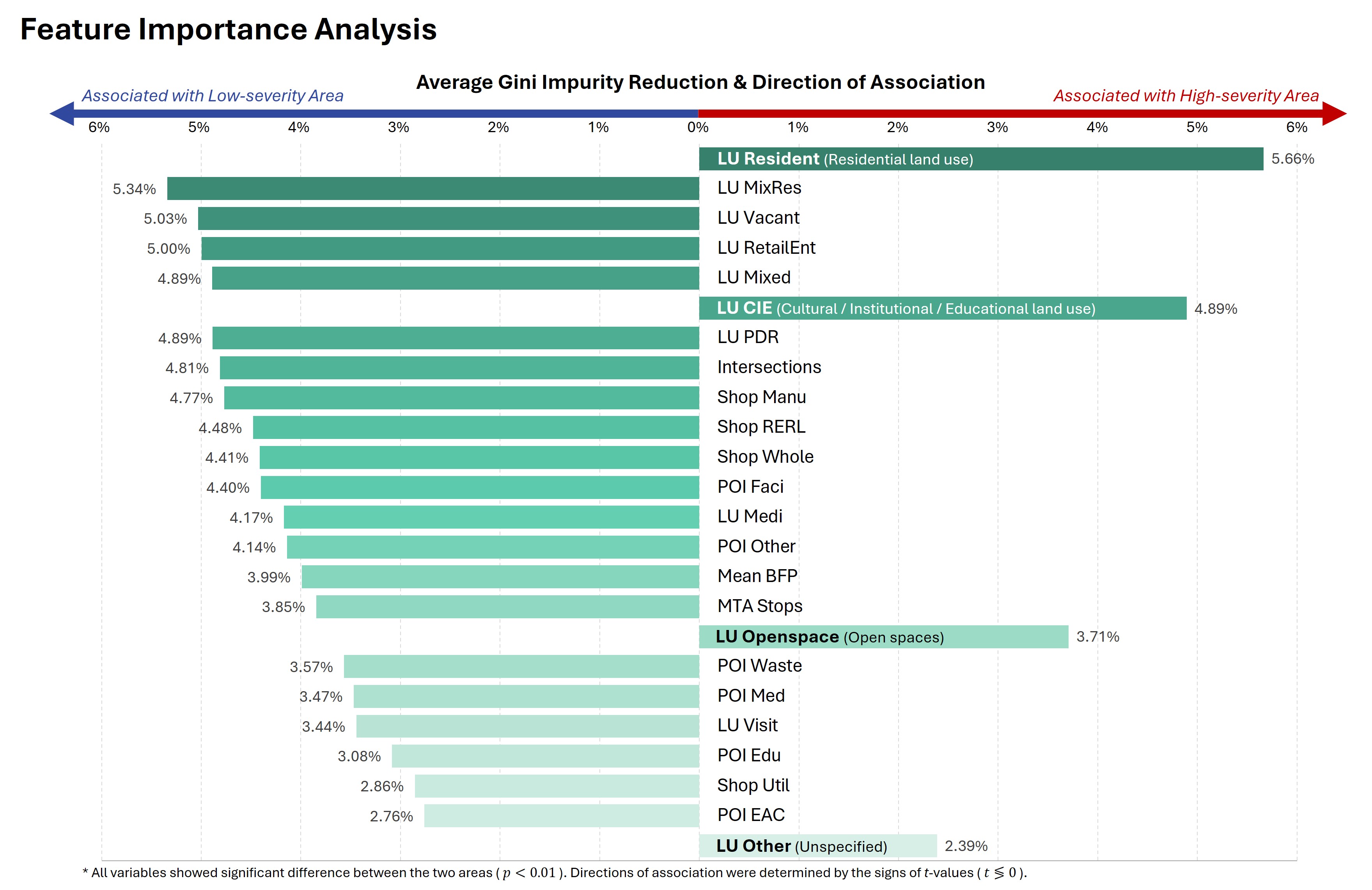
Figure 5: Feature Importance Analysis

4.3 AV Crash Severity Risk Map

We quantified and visualized the AV crash severity risk of San Francisco. The resulting map from our best accuracy ($a=0.5$) GRF model is as Figure 6. Green locations are where high-severity crashes are predicted to be less likely, and red locations are where high-severity crashes are predicted to be more likely. In general, high-severity predictions were more frequent in western residential areas, than in northeastern downtown areas. Distinct patches of either high-severity or low-severity locations were identified throughout the study area.

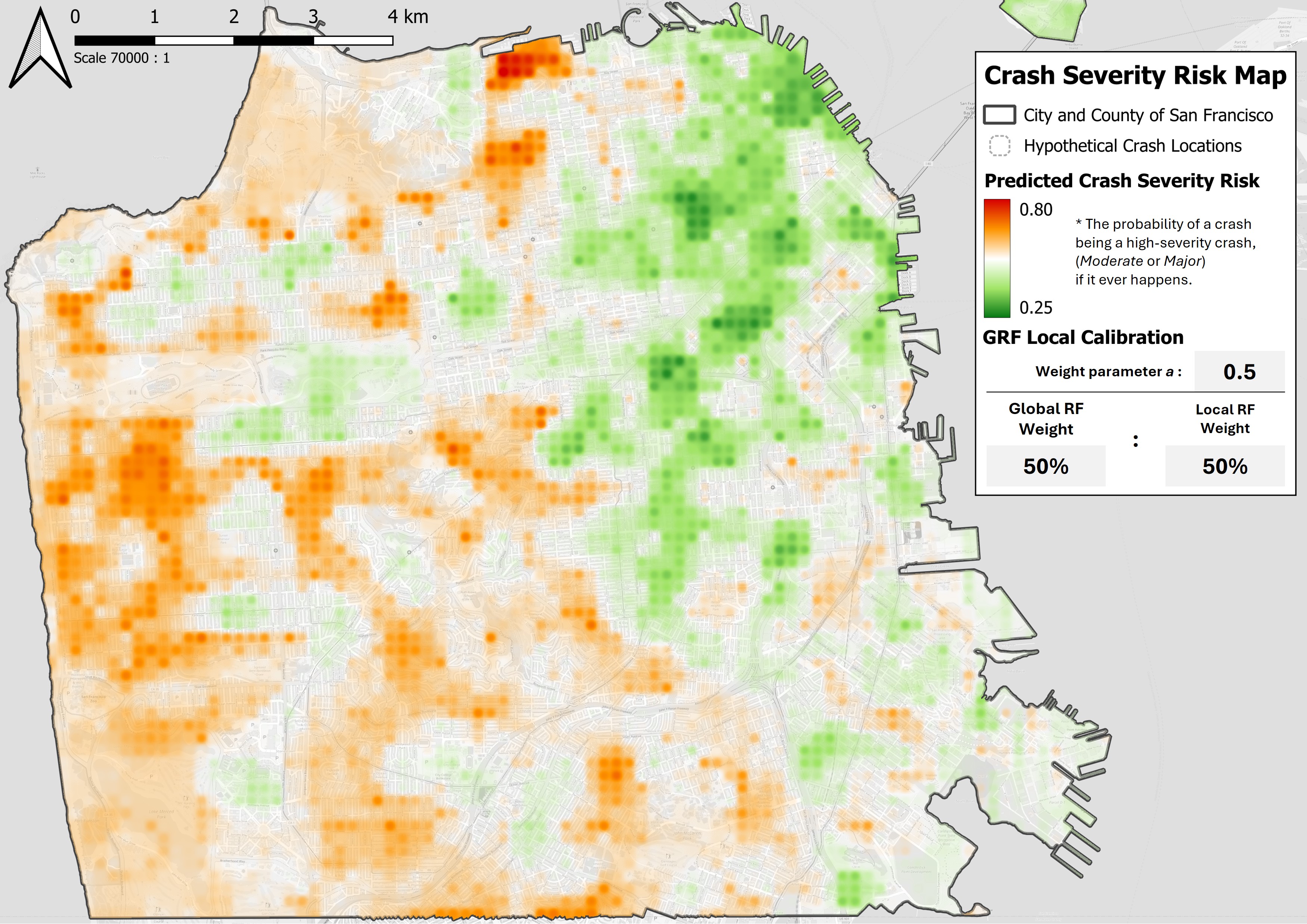
Figure 6: Crash Severity Risk Map of San Francisco

5 Discussion

5.1 Effects of Geographical Random Forest

We could perform a controlled comparison between global RF and localized RF. When all else remains the same, adjusting the weight parameter $a$ significantly impacted model performance. Despite different localization weights similarly explained the variability in data ($R^{2}$), it was possible for GRF models ($a>0.01$) to show better performance than regular RF ($a=0.01$) models, in either overall accuracy (50% localization) or recall (16% localization). This suggests that AV crash severity exhibits spatial heterogeneity and spatial autocorrelation. Geographical localization improves a machine learning model’s predictive power by capturing these spatial effects. However, predicting AV crash severity with GRF worked best if we balance between the global model and local models. Appropriately controlling the level of localization was essential.

Changing the parameter $a$ yielded varying results as Figure 7. Model (b) at 50% localization is the best accuracy model. Model (a) is the visualization made with 1% weight on local RF, and model (c) is made with 99% weight on local RF. In general, stronger localization yielded more higher and more pronounced predictions on AV crash severity. Model (c) showed more extreme predictions especially towards both higher severity. Also, predicted low-severity ‘safe zones’ were more granular and scattered across the study area.

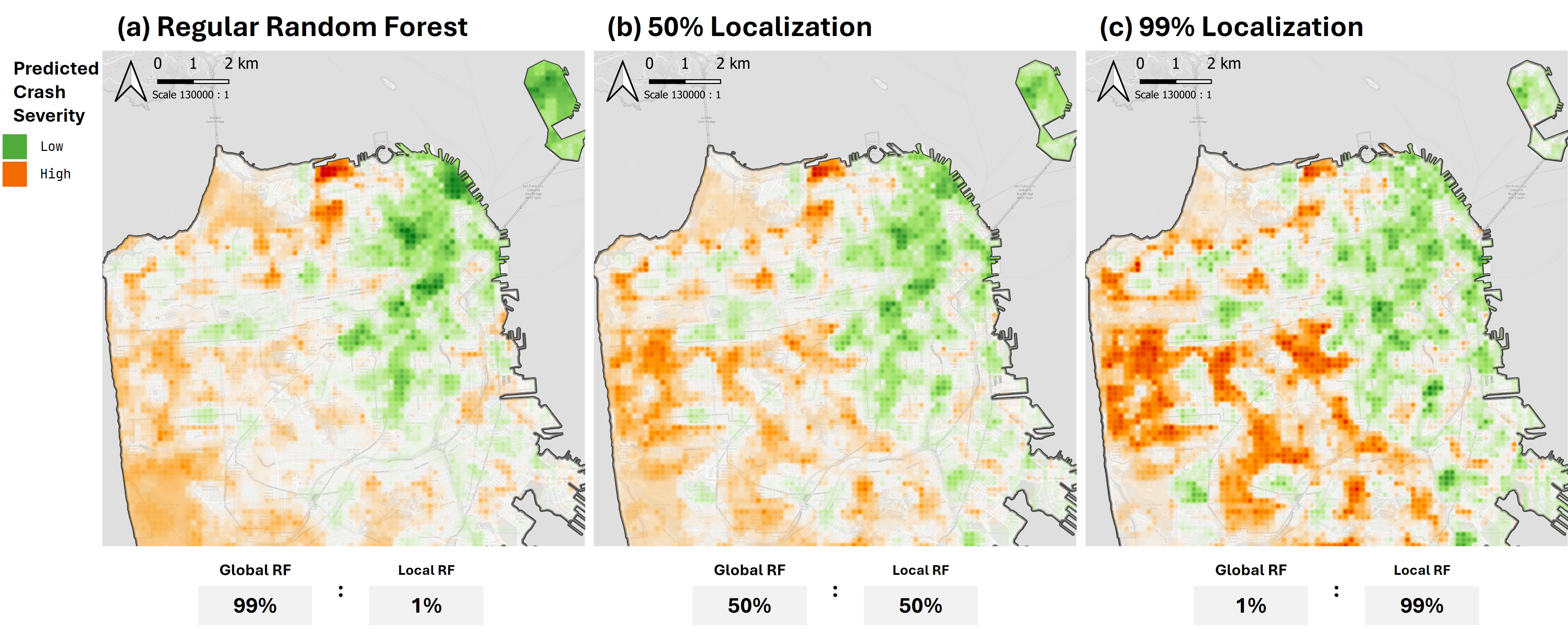
Figure 7: AV Crash Severity Risk Profiles with Varying Localization Weights; (a) Regular Random Forest; (b) 50% Localization; (c): 99% Localization

We can interpret this from a bias-variance tradeoff perspective. GRF is designed to suppress variance with a global model and suppress bias with local models [78]. Our AV crash severity risk profiles in 7 are evident that stronger localization (c) shows increased variance in crash severity risks, while weaker localization (a) shows superficial and coarse predictions. Considering that (b) had best overall accuracy at 78%, we can say that (a) resulted from underfitting and (c) resulted from overfitting. Underfitting means that the model did not sufficiently capture locally heterogeneous signals, and overfitting means that the model failed to generalize by focusing too much on local signals.

5.2 Land Use and AV Crash Severity

The feature importance analysis in Figure 5 shows that LU classification was the most important BE measure in predicting AV crash severity. Number of intersections, number of shops, POIs, and mean building footprints turned out to be relatively weak predictors. This suggests the need for AV systems to be aware of their higher level surroundings. On top of recognizing individual physical elements, the perception systems of AVs need to be fine-tuned regarding in which part of the city the system is expected to run on. Figure 5 also shows that residential LU is associated with higher AV crash severity, while commercial or mixed use LU is associated with the opposite.

In order to further support this finding, we conducted a neighborhood-level examination as Figure 8. The crash severity predictions in downtown area (a) and residential area (b) alongside parcel-level land use classification (seven highest feature importance only) are shown. LU diversity and commercial activity was noticeably greater (MixRes, Mixed, and RetailEnt LU) at low-severity locations like Lower Nob Hill and South of Market (SoMa). On the other hand, high-severity locations were dominated by uniform, rectangular tract homes (Residential LU). Also, the three small, mixed use strip malls on the east side of Outer Sunset and Parkside showed distinct low-severity clusters surrounded by high-severity predictions. Despite vehicle crashes happen more frequently in diverse commercial areas [44, 45], our analyses show that uniform residential areas can pose a greater risk on AV crash severity. Since crash frequency and crash severity are not the same, we can interpret this as the following. Once an AV crash happen in a residential area, it is expected to be more severe, compared to commercial areas.

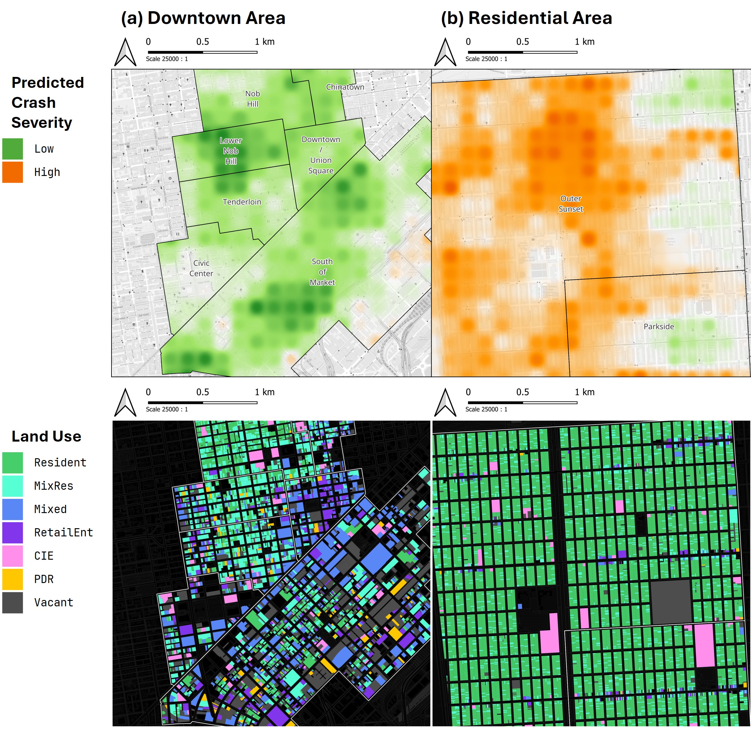
Figure 8: Land Use Comparison; (a) Downtown Area; (b) Residential Area

There are two possible reasons for this. First, residential LU may be related to certain human behaviors that lead to high-severity crashes. For instance, pedestrians in residential areas jaywalk more often, and this can be a critical cause for AV crashes [84]. AVs are less likely to react promptly if pedestrians are not expected on roads. Also, certain pedestrians including children and joggers are more likely to exhibit active behaviors, and less likely to promptly react. This is supported by the positive association of education (LU CIE) and open spaces (LU Openspace) to higher crash severity. Second, residential LU may lead AVs to exhibit certain driving characteristics that can result in high-severity crashes. The complex, congested environment in dense city centers limit the reliability of AV perception systems [54], naturally restricting its speed and freedom of movement. On the contrary, in residential areas, especially where development density is low, there are less congestion and less traffic interactions. This means that AVs can drive in higher speeds. Higher speed, in turn, leaves less time for the system to react to unforeseen obstacles. Less restrictive environment may be paradoxically causing more severe crash outcomes.

6 Conclusion

This study predicts the crash severity of Autonomous Vehicles (AVs) with Geographical Random Forest (GRF) and city scale measures of the urban built environment. This study contributes to the growing body of research on AV safety from two novel aspects. First, our spatially localized machine learning model incorporates spatial heterogeneity and spatial autocorrelation in predicting AV crash severity. Second, we investigate the higher level, city scale built environment measures including both Points Of Interests (POIs) and land use classification in predicting AV crash severity. Both aspects have not been addressed in existing AV safety research.

This study has three major findings. First, our GRF model reveals that spatially localized machine learning performs better than regular machine learning. It also highlights the importance of carefully controlling the degree of localization from a bias-variance tradeoff standpoint. Second, land use classification was most important in predicting AV crash severity, among other measures like intersections, building footprints, public transit stops, and POIs. Third, diverse commercial areas were associated with lower AV crash severity, whereas residential neighborhoods were associated with higher AV crash severity. From these findings, it is suggested that residential land use effects AV crash severity via: (1) certain behavioral patterns of pedestrians and (2) less complex environment resulting in higher AV speeds.

These findings offer two practical insights for commercial operations of AVs, especially, autonomous taxi services (robotaxi). First, robotaxi operators should incorporate geographic location when training the perception systems for their AV fleet. The system will perform better when the model localized; a set of motion planning rules which differ across geographic space can capture the latent effects from spatial heterogeneity and spatial autocorrelation. Second, even if dense city centers are more complex and diverse, it does not mean that residential neighborhoods are safer. More robust safety measures should be implemented when driving in residential neighborhoods, because if a crash ever happens, its outcome is expected to be more severe. This can include lower speed limits, more consideration of potential unsafe human behavior, and better training on such environments such as geographically localized fine-tuning on the AVs’ perception system.

There are limitations that should be addressed in subsequent research. First, our study focused exclusively on San Francisco, which has unique urban characteristics that may not generalize to other cities. Despite San Francisco having the most accessible dataset, a cross-city analysis is required to test our findings. Second, we examined crash severity without controlling for crash frequency and traffic volume, which limits our understanding of overall AV safety management. Since crash severity does not directly relate to human injury, preventing a crash from happening in the first place must also be investigated. Interpreting low-severity locations as ‘safe streets’ is not perfectly appropriate. Integrating both crash severity and crash occurrence should present a more comprehensive AV safety risk assessment.

CRediT authorship contribution statement

Junfeng Jiao: Supervision, Project administration, Funding acquisition. Seung Gyu Baik: Writing - Original Draft, Conceptualization, Methodology, Software, Visualization. Seung Jun Choi: Writing - Review & Editing, Supervision, Conceptualization, Investigation. Yiming Xu: Writing - Review & Editing, Resources, Data Curation, Validation.

Declaration of competing interest

The authors declare that they have no known competing financial interests or personal relationships that could have appeared to influence the work reported in this paper.

Data availability

The data and Python scripts used in this article are available upon request.

References

- [1] SAE International “Taxonomy and Definitions for Terms Related to Driving Automation Systems for On-Road Motor Vehicles” In SAE J3016_202104, 2021
- [2] NHTSA “Automated Vehicles for Safety” National Highway Traffic Safety Administration URL: https://www.nhtsa.gov/vehicle-safety/automated-vehicles-safety
- [3] Johannes Deichmann et al. “Autonomous driving’s future: Convenient and connected” McKinsey & Company, 2023 URL: https://www.mckinsey.com/industries/automotive-and-assembly/our-insights/autonomous-drivings-future-convenient-and-connected
- [4] Center for Sustainable Systems “Autonomous Vehicles Factsheet” University of Michigan, 2024 URL: https://css.umich.edu/publications/factsheets/mobility/autonomous-vehicles-factsheet
- [5] Henry Alexander Ignatious, Hesham El-Sayed and Manzoor Khan “An overview of sensors in Autonomous Vehicles” In Procedia Comput. Sci. 198, 2022, pp. 736–741 DOI: 10.1016/j.procs.2021.12.315
- [6] Fenglian Pan et al. “Reliability modeling for perception systems in autonomous vehicles: A recursive event-triggering point process approach” In Transp. Res. C 169, 2024, pp. 104868 DOI: 10.1016/j.trc.2024.104868
- [7] Jean-François Bonnefon, Azim Shariff and Iyad Rahwan “The social dilemma of autonomous vehicles” In Science 352, 2016, pp. 1573–1576 DOI: 10.1126/science.aaf2654
- [8] James M. Anderson et al. “Autonomous Vehicle Technology: A Guide for Policymakers”, 2016 URL: https://www.rand.org/pubs/research_reports/RR443-2.html
- [9] Daniel J. Fagnant and Kara Kockelman “Preparing a nation for autonomous vehicles: opportunities, barriers and policy recommendations” In Transp. Res. A 77 Pergamon, 2015, pp. 167–181 DOI: 10.1016/J.TRA.2015.04.003
- [10] Hye Min Park and Fabian Villalobos “Reining in the Risks of Robotaxis” RAND Corporation, 2024 URL: https://www.governing.com/policy/reining-in-the-risks-of-robotaxis
- [11] Peter André Busch “Non-user acceptance of autonomous technology: A survey of bicyclist receptivity to fully autonomous vehicles” In Comput. Hum. Behav. Rep. 16 Elsevier, 2024, pp. 100490 DOI: 10.1016/J.CHBR.2024.100490
- [12] NHTSA “ADS Incident Report Data” National Highway Traffic Safety Administration, 2025 URL: https://www.nhtsa.gov/laws-regulations/standing-general-order-crash-reporting#data
- [13] Goldman Sachs “Partially autonomous cars forecast to comprise 10% of new vehicle sales by 2030”, 2024 URL: https://www.goldmansachs.com/insights/articles/partially-autonomous-cars-forecast-to-comprise-10-percent-of-new-vehicle-sales-by-2030
- [14] Francesca M. Favarò et al. “Examining accident reports involving autonomous vehicles in California” In PLOS ONE 12, 2017, pp. e0184952 DOI: 10.1371/journal.pone.0184952
- [15] Chengcheng Xu, Zijian Ding, Chen Wang and Zhibin Li “Statistical analysis of the patterns and characteristics of connected and autonomous vehicle involved crashes” In J. Safety. Res. 71, 2019, pp. 41–47 DOI: 10.1016/j.jsr.2019.09.001
- [16] Yixuan Li, Xuesong Wang, Tianyi Wang and Qian Liu “Characteristics Analysis of Autonomous Vehicle Pre-crash Scenarios”, 2025 arXiv: https://arxiv.org/abs/2502.20789
- [17] Teshome Kumsa Kurse, Girma Gebresenbet, Geleta Fikadu Daba and Negasa Tesfaye Tefera “Experimental determination of factors causing crashes involving automated vehicles” In Multimodal Transp. 4 Elsevier, 2025, pp. 100186 DOI: 10.1016/J.MULTRA.2024.100186
- [18] Hanlong Fu et al. “New insights into factors affecting the severity of autonomous vehicle crashes from two sources of AV incident records” In Travel Behav. Soc. 38 Elsevier, 2025, pp. 100934 DOI: 10.1016/J.TBS.2024.100934
- [19] Jorge Vargas et al. “An Overview of Autonomous Vehicles Sensors and Their Vulnerability to Weather Conditions” In Sensors 21, 2021, pp. 5397 DOI: 10.3390/s21165397
- [20] Mohamed Abdel-Aty and Shengxuan Ding “A matched case-control analysis of autonomous vs human-driven vehicle accidents” In Nat. Commun. 15, 2024, pp. 4931 DOI: 10.1038/s41467-024-48526-4
- [21] United States Environmental Protection Agency “Basic Information about the Built Environment” United States Environmental Protection Agency, 2025 URL: https://www.epa.gov/smm/basic-information-about-built-environment
- [22] Adriana Araujo Portella “Built Environment” In Encyclopedia of Quality of Life and Well-Being Research Springer Netherlands, 2014, pp. 454–461 DOI: 10.1007/978-94-007-0753-5˙240
- [23] Nancy Hepp and Lorelei Walker “Built Environment” Collaborative for Health & Environment, 2016 URL: https://www.healthandenvironment.org/resources/environmental-hazards/exposure-sources/built-environment
- [24] Benoît Flahaut “Impact of infrastructure and local environment on road unsafety: Logistic modeling with spatial autocorrelation” In Accid. Anal. Prev. 36 Pergamon, 2004, pp. 1055–1066 DOI: 10.1016/J.AAP.2003.12.003
- [25] Peijie Wu, Li Song and Xianghai Meng “Influence of built environment and roadway characteristics on the frequency of vehicle crashes caused by driver inattention: A comparison between rural roads and urban roads” In J. Safety. Res. 79 Pergamon, 2021, pp. 199–210 DOI: 10.1016/J.JSR.2021.09.001
- [26] Wesley Earl Marshall and Norman W. Garrick “Does street network design affect traffic safety?” In Accid. Anal. Prev. 43, 2011, pp. 769–781 DOI: 10.1016/j.aap.2010.10.024
- [27] Nicholas N. Ferenchak and Wesley E. Marshall “Traffic safety for all road users: A paired comparison study of small & mid-sized U.S. cities with high/low bicycling rates” In J. Cycl. Micromobility Res. 2 Elsevier, 2024, pp. 100010 DOI: 10.1016/J.JCMR.2024.100010
- [28] Reid Ewing and Eric Dumbaugh “The built environment and traffic safety: A review of empirical evidence” In J. Plan. Lit. 23, 2009, pp. 347–367 DOI: 10.1177/0885412209335553
- [29] Yiping Liu et al. “Is there an emotional dimension to road safety? A spatial analysis for traffic crashes considering streetscape perception and built environment” In Anal. Methods Accid. Res. 46, 2025, pp. 100374 DOI: 10.1016/j.amar.2025.100374
- [30] United States Environmental Protection Agency “Land Use” United States Environmental Protection Agency, 2025 URL: https://www.epa.gov/report-environment/land-use
- [31] Eric Dumbaugh and Wenhao Li “Designing for the Safety of Pedestrians, Cyclists, and Motorists in Urban Environments” In J. Am. Plan. Assoc. 77, 2010, pp. 69–88 DOI: 10.1080/01944363.2011.536101
- [32] Satish Ukkusuri, Luis F. Miranda-Moreno, Gitakrishnan Ramadurai and Jhael Isa-Tavarez “The role of built environment on pedestrian crash frequency” In Saf. Sci. 50 Elsevier, 2012, pp. 1141–1151 DOI: 10.1016/J.SSCI.2011.09.012
- [33] Huiwen Liu, Weihua Zhang, Zeyang Cheng and Tengfei Wang “Investigating the contributing factors of urban crash levels: A novel stacking integrated learning framework” In Appl. Geogr. 173 Pergamon, 2024, pp. 103440 DOI: 10.1016/J.APGEOG.2024.103440
- [34] Pei-Fen Kuo, Umroh Dian Sulistyah, I Gede Brawiswa Putra and Dominique Lord “Exploring the spatial relationship of e-bike and motorcycle crashes: Implications for risk reduction” In J. Safety. Res. 88, 2024, pp. 199–216 DOI: 10.1016/j.jsr.2023.11.007
- [35] Robert Cervero “Mixed land-uses and commuting: Evidence from the American Housing Survey” In Transp. Res. A 30 Pergamon, 1996, pp. 361–377 DOI: 10.1016/0965-8564(95)00033-X
- [36] Zhuo Yang et al. “Analysis of Washington, DC taxi demand using GPS and land-use data” In J. Transp. Geogr. 66 Pergamon, 2018, pp. 35–44 DOI: 10.1016/J.JTRANGEO.2017.10.021
- [37] Junyong Choi, Wonjun No, Minju Park and Youngchul Kim “Inferring land use from spatialtemporal taxi ride data” In Appl. Geogr. 142 Pergamon, 2022, pp. 102688 DOI: 10.1016/J.APGEOG.2022.102688
- [38] Song Gao, Yingjie Hu and Wenwen Li “Heterogeneity-Aware Deep Learning in Space: Performance and Fairness” In Handbook of Geospatial Artificial Intelligence CRC Press, 2023, pp. 151–176 DOI: 10.1201/9781003308423
- [39] Gengchen Mai et al. “Towards the next generation of Geospatial Artificial Intelligence” In Int. J. Appl. Earth Obs. Geoinf. 136, 2025, pp. 104368 DOI: 10.1016/j.jag.2025.104368
- [40] Luc Anselin “Spatial Econometrics: Methods and Models” Springer Netherlands, 1988 DOI: 10.1007/978-94-015-7799-1
- [41] James LeSage and Robert Kelley Pace “Introduction” In Introduction to Spatial Econometrics ChapmanHall/CRC, 2009, pp. 1–24 DOI: 10.1201/9781420064254
- [42] Shuli Wang et al. “Geographically weighted machine learning for modeling spatial heterogeneity in traffic crash frequency and determinants in US” In Accid. Anal. Prev. 199, 2024, pp. 107528 DOI: 10.1016/j.aap.2024.107528
- [43] Tian Li et al. “Spatial heterogeneity effect of built environment on traffic safety using geographically weighted atrous convolutions neural network” In Accid. Anal. Prev. 213, 2025, pp. 107934 DOI: 10.1016/j.aap.2025.107934
- [44] Ahmed Osama and Tarek Sayed “Evaluating the Impact of Socioeconomics, Land Use, Built Environment, and Road Facility on Cyclist Safety” In Transp. Res. Rec. 2659, 2017, pp. 33–42 DOI: 10.3141/2659-04
- [45] Yuan Huang, Xiaoguang Wang and David Patton “Examining spatial relationships between crashes and the built environment: A geographically weighted regression approach” In J. Transp. Geogr. 69, 2018, pp. 221–233 DOI: 10.1016/j.jtrangeo.2018.04.027
- [46] Louis A. Merlin, Erick Guerra and Eric Dumbaugh “Crash risk, crash exposure, and the built environment: A conceptual review” In Accid. Anal. Prev. 134 Pergamon, 2020, pp. 105244 DOI: 10.1016/J.AAP.2019.07.020
- [47] Dong Xiao, Hongliang Ding, N N Sze and Nan Zheng “Investigating built environment and traffic flow impact on crash frequency in urban road networks” In Accid. Anal. Prev. 201, 2024, pp. 107561 DOI: 10.1016/j.aap.2024.107561
- [48] D.W. Wong “Modifiable Areal Unit Problem” In International Encyclopedia of Human Geography Elsevier, 2009, pp. 169–174 DOI: 10.1016/B978-008044910-4.00475-2
- [49] Hongliang Ding et al. “Quantifying the heterogeneity impact of risk factors on regional bicycle crash frequency: A hybrid approach of clustering and random parameter model” In Accid. Anal. Prev. 207, 2024, pp. 107753 DOI: 10.1016/j.aap.2024.107753
- [50] Swagata Sarkar et al. “Determination of Various Risk Elements’ Association Causing Fatal Crashes in Heterogeneous Traffic Conditions” In Transp. Res. Rec., 2025 DOI: 10.1177/03611981241312221
- [51] Boniphace Kutela, Subasish Das and Bahar Dadashova “Mining patterns of autonomous vehicle crashes involving vulnerable road users to understand the associated factors” In Accid. Anal. Prev. 165 Pergamon, 2022, pp. 106473 DOI: 10.1016/J.AAP.2021.106473
- [52] Pei Li et al. “Analyzing relationships between latent topics in autonomous vehicle crash narratives and crash severity using natural language processing techniques and explainable XGBoost” In Accid. Anal. Prev. 203, 2024, pp. 107605 DOI: 10.1016/j.aap.2024.107605
- [53] Siying Zhu and Qiang Meng “What can we learn from autonomous vehicle collision data on crash severity? A cost-sensitive CART approach” In Accid. Anal. Prev. 174, 2022, pp. 106769 DOI: 10.1016/j.aap.2022.106769
- [54] Hengrui Chen et al. “Analysis of Factors Affecting the Severity of Automated Vehicle Crashes Using XGBoost Model Combining POI Data” In J. Adv. Transp. 2020, 2020, pp. 1–12 DOI: 10.1155/2020/8881545
- [55] Weixi Ren, Bo Yu, Yuren Chen and Kun Gao “Divergent Effects of Factors on Crash Severity under Autonomous and Conventional Driving Modes Using a Hierarchical Bayesian Approach” In Int. J. Environ. Res. Public Health 19, 2022, pp. 11358 DOI: 10.3390/ijerph191811358
- [56] Pei-Fen Kuo, Wei-Ting Hsu, Dominique Lord and I Gede Brawiswa Putra “Classification of autonomous vehicle crash severity: Solving the problems of imbalanced datasets and small sample size” In Accid. Anal. Prev. 205, 2024, pp. 107666 DOI: 10.1016/j.aap.2024.107666
- [57] Robert Cervero and Kara Kockelman “Travel demand and the 3Ds: Density, diversity, and design” In Transp. Res. D 2 Pergamon, 1997, pp. 199–219 DOI: 10.1016/S1361-9209(97)00009-6
- [58] Reid Ewing and Robert Cervero “Travel and the Built Environment: A Synthesis” In Transp. Res. Rec. 1780, 2001, pp. 87–114 DOI: 10.3141/1780-10
- [59] Susan Handy “Enough with the “Ds” Already — Let’s Get Back to “A”” Transfers Magazine, 2018 URL: https://transfersmagazine.org/magazine-article/issue-1/enough-with-the-ds-already-lets-get-back-to-a/
- [60] Eric Dumbaugh and Robert Rae “Safe urban form: Revisiting the relationship between community design and traffic safety” In J. Am. Plan. Assoc. 75, 2009, pp. 309–329 DOI: 10.1080/01944360902950349
- [61] Xiang Liu, Xiaohong Chen, Mingshu Tian and Jonas De Vos “Effects of buffer size on associations between the built environment and metro ridership: A machine learning-based sensitive analysis” In J. Transp. Geogr. 113, 2023, pp. 103730 DOI: 10.1016/j.jtrangeo.2023.103730
- [62] Clarence Arthur Perry “The Neighborhood Unit: A Scheme of Arrangement for the Family Life Community” In Regional Plan for New York and Its Environs 7, 1929
- [63] Michael W. Mehaffy, Sergio Porta and Ombretta Romice “The “neighborhood unit” on trial: a case study in the impacts of urban morphology” In J. Urban. Int. Res. Placemaking Urban Sustain. 8, 2015, pp. 199–217 DOI: 10.1080/17549175.2014.908786
- [64] Robert Cervero and Erick Guerra “Urban Densities and Transit: A Multi-dimensional Perspective” In Institute of Transportation Studies, University of California, Berkeley Institute of Transportation Studies, University of California, Berkeley, 2011
- [65] PSRC “Transit-Supportive Densities and Land Uses” Puget Sound Regional Council, 2015, pp. 13–37 URL: https://www.psrc.org/sites/default/files/2022-03/tsdluguidancepaper.pdf
- [66] Reid Ewing “Contribution of Urban Design Qualities to Pedestrian Activity” In Planning Magazine, 2016 URL: https://planning.org/planning/2016/feb/research.htm
- [67] Douglas C. Montgomery and George C. Runger “Nonparametric Procedures” In Applied Statistics and Probability for Engineers 7th ed., 2018, pp. 234–240
- [68] Tae Kyun Kim and Jae Hong Park “More about the basic assumptions of t-test: normality and sample size” In Korean J. Anesthesiol. 72, 2019, pp. 331–335 DOI: 10.4097/kja.d.18.00292
- [69] Gareth James, Daniela Witten, Trevor Hastie and Robert Tibshirani “Linear Regression” In An Introduction to Statistical Learning Springer, 2021, pp. 59–128 DOI: 10.1007/978-1-0716-1418-1˙3
- [70] Haibo He and E.A. Garcia “Learning from Imbalanced Data” In IEEE Trans. Knowl. Data Eng. 21, 2009, pp. 1263–1284 DOI: 10.1109/TKDE.2008.239
- [71] Bartosz Krawczyk “Learning from imbalanced data: open challenges and future directions” In Prog. Artif. Intell. 5, 2016, pp. 221–232 DOI: 10.1007/s13748-016-0094-0
- [72] N.. Chawla, K.. Bowyer, L.. Hall and W.. Kegelmeyer “SMOTE: Synthetic Minority Over-sampling Technique” In J. Artif. Intell. 16, 2002, pp. 321–357 DOI: 10.1613/jair.953
- [73] Brian A. Johnson and Kotaro Iizuka “Integrating OpenStreetMap crowdsourced data and Landsat time-series imagery for rapid land use/land cover (LULC) mapping: Case study of the Laguna de Bay area of the Philippines” In Appl. Geogr. 67, 2016, pp. 140–149 DOI: 10.1016/j.apgeog.2015.12.006
- [74] Yonghong Zhang, Taotao Ge, Wei Tian and Yuei-An Liou “Debris Flow Susceptibility Mapping Using Machine-Learning Techniques in Shigatse Area, China” In Remote Sens. 11, 2019, pp. 2801 DOI: 10.3390/rs11232801
- [75] Leo Breiman “Random Forests” In Mach. Learn. 45, 2001, pp. 5–32 DOI: 10.1023/A:1010933404324
- [76] Peijun Du et al. “Random Forest and Rotation Forest for fully polarized SAR image classification using polarimetric and spatial features” In ISPRS J. Photogramm. Remote Sens. 105, 2015, pp. 38–53 DOI: 10.1016/j.isprsjprs.2015.03.002
- [77] Meisam Amani et al. “Google Earth Engine Cloud Computing Platform for Remote Sensing Big Data Applications: A Comprehensive Review” In IEEE J. Sel. Top. Appl. Earth. Obs. Remote Sens. 13, 2020, pp. 5326–5350 DOI: 10.1109/JSTARS.2020.3021052
- [78] Stefanos Georganos et al. “Geographical random forests: a spatial extension of the random forest algorithm to address spatial heterogeneity in remote sensing and population modelling” In Geocarto Int. 36, 2021, pp. 121–136 DOI: 10.1080/10106049.2019.1595177
- [79] Jesús Aguirre-Gutiérrez et al. “Pantropical modelling of canopy functional traits using Sentinel-2 remote sensing data” In Remote Sens. Environ. 252, 2021, pp. 112122 DOI: 10.1016/j.rse.2020.112122
- [80] B. Sailaja et al. “Spatial temperature prediction—a machine learning and GIS perspective” In Theor. Appl. Climatol. 155, 2024, pp. 9619–9642 DOI: 10.1007/s00704-024-05167-3
- [81] Weisheng Lu, Bing Yang, Liang Yuan and Ziyu Peng “Understanding fly-tipping in urban areas: A social-economic-spatial combinatorial approach enabled by geographically weighted random forest” In Environ. Impact Assess. Rev. 112, 2025, pp. 107858 DOI: 10.1016/j.eiar.2025.107858
- [82] Dongyu Wu, Yingheng Zhang and Qiaojun Xiang “Geographically weighted random forests for macro-level crash frequency prediction” In Accid. Anal. Prev. 194, 2024, pp. 107370 DOI: 10.1016/j.aap.2023.107370
- [83] Kai Sun, Ryan Zhenqi Zhou, Jiyeon Kim and Yingjie Hu “PyGRF: An Improved Python Geographical Random Forest Model and Case Studies in Public Health and Natural Disasters” In Trans. GIS 28, 2024, pp. 2476–2491 DOI: 10.1111/tgis.13248
- [84] Ziqian Zhang et al. “Decision-making of autonomous vehicles in interactions with jaywalkers: A risk-aware deep reinforcement learning approach” In Accid. Anal. Prev. 210, 2025, pp. 107843 DOI: 10.1016/j.aap.2024.107843