Quantifying uncertainty and stability among highly correlated predictors: a subspace perspective

Abstract.

We study the problem of linear feature selection when features are highly correlated. This setting presents two main challenges. First, how should false positives be defined? Intuitively, selecting a null feature that is highly correlated with a true one may be less problematic than selecting a completely uncorrelated null feature. Second, correlation among features can cause variable selection methods to produce very different feature sets across runs, making it hard to identify stable features. To address these issues, we propose a new framework based on feature subspaces – the subspaces spanned by selected columns of the feature matrix. This framework leads to a new definition of false positives and negatives based on the “similarity” of feature subspaces. Further, instead of measuring stability of individual features, we measure stability with respect to feature subspaces. We propose and theoretically analyze a subspace generalization of stability selection (Meinshausen and Bühlmann, 2010). This procedure outputs multiple candidate stable models which can be considered interchangeable due to multicollinearity. We also propose a method for identifying substitute structures – features that can be swapped and yield “equivalent” models. Finally, we demonstrate our framework and algorithms using both synthetic and real gene expression data. Our methods are implemented in the R package substab.

1. Introduction

Variable selection is a perennial problem in data science. Given a large set of features, the objective is to identify a small subset that is predictive of a response variable of interest. Despite the massive amount of work in this area, variable selection in highly correlated settings remains a significant challenge.

One challenge is assessing the quality of model selection in terms of false positive and false negative errors. Traditionally, false positive error or false negative error corresponds to the number of features that are incorrectly included or excluded in the model. As a simple illustration of the challenge with the traditional perspective on false positive/negative error, suppose our data consists of two features $X_{1},X_{2}$ that are nearly identical up to a small measurement noise, where $X_{1}$ is a signal variable and $X_{2}$ is a null (non-signal) variable. Unless the sample size is very large and the signal-to-noise ratio is high, variable selection methods such as Lasso may select the null variable over the signal variable. In the case where $X_{2}$ is selected over $X_{1}$, we incur one false positive error and one false negative error. Intuitively, however, selecting a feature nearly identical to a truly relevant variable should not incur a false positive/negative error of one, but rather a false positive/negative error of nearly zero.

A second challenge is measuring stability of feature selection procedures. The importance of stability is highlighted in Yu and Kumbier (2020) and Yu (2013), which uses the term to refer to when “statistical conclusions are robust or stable to appropriate perturbations to data.” A widely used stability-based procedure in regression is stability selection (Meinshausen and Bühlmann, 2010). The basic idea is that instead of applying one’s favorite variable selection algorithm such as the Lasso to the whole data set, one instead applies it several times to random subsamples of the data. The proportion of subsamples where each feature is selected then represents the stability of that feature; the features can then be ranked according to their stability. Consider the previous toy illustration. Due to the high correlation of $X_{1}$ and $X_{2}$, nearly half of the subsamples in the stability selection procedure would select feature $X_{1}$ and the other half $X_{2}$ (Faletto and Bien, 2022). This “vote splitting” (Shah and Samworth, 2013) may result in neither $X_{1}$ nor $X_{2}$ being ranked highly by stability selection, despite their relationship with $Y$. Ideally, we would want to give a large stability value to both $X_{1}$ and $X_{2}$.

Building on stability, a third challenge is how to aggregate stable features to output a model. To illustrate this challenge, consider the following toy setup with four features: $X_{1},X_{2},X_{3},X_{4}$, where $X_{1}$ and $X_{3}$ are signal features, and $X_{2}$ and $X_{4}$ are highly correlated with $X_{1}$ and $X_{3}$, respectively. Assuming that we have addressed the second challenge, we may find that all the features are stable. However, these four features should not be combined in a single model as having $X_{1}$ and $X_{2}$, or $X_{3}$ and $X_{4}$ together in a single model would be redundant. Indeed, it is arguably more natural to output multiple stable models including $(X_{1},X_{3})$, $(X_{1},X_{4})$, $(X_{2},X_{3})$, and $(X_{2},X_{4})$. Ideally, we would also communicate that certain features are “substitutes”; they can be swapped and yield an “equivalent” model. Outputting these sets and substitutes provides a more accurate sense of uncertainty over the variable selection procedure. This challenge motivates the following questions: (i) how do we find stable models (rather than stable features)? (ii) how do we efficiently find multiple stable models, given a large model space? (iii) how do we identify substitutes among our multiple stable sets?

In this paper, we propose a framework based on subspaces to address the aforementioned challenges. Throughout, unless otherwise specified, we use the terminology “highly correlated” to mean that the predictors $X$ are (nearly) linearly dependent. The dependency structure we consider can be much more general and complex than simply a high pairwise correlation among some predictors.

1.1. Our Contributions

As our first contribution, we propose in Section 2 a subspace perspective for assessing model selection in highly correlated settings. Suppose $X$ is a data matrix of predictors where columns index features and rows index samples. Instead of quantifying performance in terms of a set of features $\widehat{S}$, we quantify performance in terms of a feature subspace $\mathrm{col}(X_{\widehat{S}})$ – the subspace spanned by the columns of the matrix $X$ corresponding to these features. We then represent false positive and false negative errors in terms of the degree of misalignment between the estimated feature subspace $\mathrm{col}(X_{\widehat{S}})$ and the population feature subspace $\mathrm{col}(X_{S^{\star}})$, where $S^{\star}$ is the set of signal features. These subspace-based metrics reduce to the classical notions of false positive and false negative error when features are orthogonal but give more meaningful answers in highly correlated settings. The subspace perspective also enables natural measures of stability. In particular, given access to estimates $\widehat{S}^{(\ell)}(\ell=1,2,\dots,B)$, we measure stability of a feature $X_{j}$ as the degree of alignment between the subspace $\mathrm{col}(X_{j})$ and the subspaces $\mathrm{col}(X_{\widehat{S}^{(\ell)}})$; this idea can also be generalized to find the stability of a set of features. When the features are orthogonal, this metric simplifies to traditional stability measure, but it provides more meaningful measure in highly correlated settings. Finally, we can use our subspace perspective to measure the extent to which two sets of features are substitutes, i.e., capture similar components of the response variable when used as predictors.

As our second contribution, we propose in Section 3 the algorithm feature subspace stability selection (FSSS), a procedure for enumerating stable models. Similar to stability selection, as input, FSSS takes selected features $\widehat{S}^{(\ell)}(\ell=1,2,\dots,B)$ after deploying one’s favorite variable selection procedure on subsamples of the data. After mapping each subset to a subspace $\mathrm{col}(X_{\widehat{S}^{(\ell)}})$, FSSS uses a sequential procedure to obtain a collection of stable models, where each model maps to a feature subspace that is “close to” most of the estimated subspaces; the specific measure of distance here is based on the stability formalism described earlier. Since the output of FSSS can consist of many selection sets, we use our measure of substitutes to identify features (contained in the selection sets) that are good substitutes.

In Section 4, we analyze the theoretical performance of FSSS. We focus our analysis in the setting where the features can be grouped into highly correlated clusters; and describe generalizations to more complex dependency structures in the appendix. We provide false positive error guarantees for any model selected by FSSS, where the bound on the error depends on the “quality of the base procedure”. Under some assumptions on the base procedure, we show that FSSS has feature selection consistency: it returns all “equivalent” selection sets consisting of one feature from each signal cluster (a cluster containing a signal feature) and no feature from a non-signal cluster is selected.

Finally, in Section 5, we contrast FSSS with other stability selection variants using synthetic and real data. The real data analysis is a biological application involving gene expression data. FSSS shows improvements in several ways. First, in a number of synthetic experiments, as compared to other stability procedures, FSSS achieves the lowest test mean squared error and false positive error, while also producing the most consistent selection sets across different runs. In real data, FSSS performs similarly or better in predictions and selects larger feature sets. Finally, FSSS produces multiple stable models and identifies substitute structures that are meaningful in both synthetic and real data experiments, while other methods produce only one stable model.

Our methods are implemented in the R package substab. Our package provides two primary functionalities: $(i)$ Subsampling and FSSS, which takes as input a dataset of features and a response variable and outputs a collection of stable models; $(ii)$ Substitute structure discovery, which searches through these stable models and returns a list of substitute structures to help interpret the selected models.

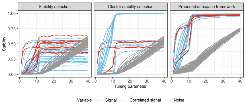
Figure 1. Stability paths of the base procedure $\ell_{0}$-penalized regression on a synthetic dataset (see Appendix C.1 for details). From left to right: stability values using stability selection, cluster stability selection, and our proposed subspace framework for different choice of tuning parameter in the base procedure. The “signal” refers to features directly generating the response. The “correlated signal” refers to features that are highly correlated with the signals. The “noise” refers to features independent of signals.

1.2. Related Work

In the last decade there has been some work devoted to tackling different aspects of the variable selection problem under high feature correlation. For example, Bühlmann et al. (2013) propose a feature selection method designed for the setting in which there are clusters of highly correlated features; however, this work does not address questions of stability or the inadequacy of traditional measures of false positive errors when features are highly correlated.

G’Sell et al. (2013) tackle this latter challenge by quantifying false positives as features in the selected model that can be explained by other features in the selected model. While in some highly correlated settings, this new metric provides more reasonable values than the standard notion, it typically gives smaller false positive errors than one may expect; see Appendix A.4.

Cluster stability selection (CSS; Faletto and Bien 2022, and Alexander and Lange 2011) is a recent method designed to improve stability selection. CSS uses a pre-defined cluster assignment of features and calculates the selection probability for each cluster. A cluster is considered selected by a subsample if any of its features are selected. CSS gathers votes from the features in each cluster, then ranks them based on the cluster’s selection probability. When features are well-clustered (either orthogonal or highly correlated), CSS helps avoid the “vote splitting” issue in stability selection. However, CSS may perform poorly in more complex settings. Figure 1 compares CSS, stability selection, and our proposed subspace framework in a setting with more complex feature correlations. While CSS partially improves upon stability selection’s performance, it still fails to identify signal variables; only our method is able to completely distinguish between noise and non-noise features.

Approaches based on principal components analysis (Bair et al., 2006, Yu et al., 2006) are widely used in highly correlated settings. These methods identify a few principal components of the feature matrix and use them to predict the response. However, since principal components are typically linear combinations of many features, they can be less interpretable than directly selecting a small number of features from the original set, which is the task considered in this paper.

High feature correlation undermines the value of finding a unique “best” model and leads, as we do here, to thinking about a set of good models. This connects our work to Breiman’s notion of the Rashomon effect (Breiman, 2001), which acknowledges that there may be a “multitude of different descriptions” of models that all achieve close to the best performance. A growing literature considers the Rashomon effect (Fisher et al., 2019, Dong and Rudin, 2020, Zhong et al., 2023). In fact, Breiman (2001) discusses stability (or rather instability) in this context. Some recent work has explicitly considered stability in the context of this multitude of models (Kissel and Mentch, 2024, Adrian et al., 2024), although neither focuses on subspaces in the way that our work does.

1.3. Notation

For a subspace $T\subseteq\mathbb{R}^{n}$, we denote the projection onto $T$ by $\mathcal{P}_{T}$. The subspace consisting of all vectors that are orthogonal to those in $T$ are denoted by $T^{\perp}$. For a matrix $M\in\mathbb{R}^{m\times m}$, we denote the span of the columns of $M$ (i.e. its column space) by $\mathrm{col}(M)$. We denote the singular values of $M$, in descending order by $\sigma_{1},\sigma_{2},\dots,\sigma_{m}$. For a set $S\subseteq\{1,2,\dots,p\}$, we denote $S^{c}$ as its complement.

2. Why are subspaces useful?

Setup: Let $X\in\mathbb{R}^{n\times p}$ represent the data matrix of predictors where columns index the $p$ features and rows index the $n$ samples. Let $y\in\mathbb{R}^{n}$ encode observations of the response variable. Throughout, we consider linear regression models in which linear combinations of features are used to predict the response; we discuss extensions to generalized linear models in Appendix A.2. We assume that the features are centered, so that the sum of entries in every column in $X$ is zero.

This section is organized as follows: Section 2.1 gives a brief description of what it means to represent selection sets as subspaces; Section 2.2 describes how a subspace perspective enables a natural measure of false positive and false negative error in highly correlated settings; Section 2.3 describes a measure of stability using subspaces; and finally, as multiple models may be simultaneously stable, Section 2.4 presents methods to detect substitute structures among stable models.

2.1. Representing selection sets as subspaces

Consider two regression models. The first uses the features $X_{1}$ and $X_{2}$ to predict the response, and the second uses $X_{3}$ and $X_{4}$. A common perspective is to represent the first model’s structure as the selection set $S=\{1,2\}$ and the second as $\widetilde{S}=\{3,4\}$. Since the sets $S$ and $\widetilde{S}$ are disjoint, the two model structures would be viewed as having nothing in common. Two observations can be made here. First, suppose that $X_{1}$ and $X_{3}$ are identical up to small measurement noise, and $X_{2}$ and $X_{4}$ are identical up to small measurement noise. In this highly correlated setting, contrary to the conclusion made earlier, our two model structures have significant commonalities: linear combinations of $X_{1}$ and $X_{2}$ are very close to linear combinations of $X_{3}$ and $X_{4}$. Second, the comparison of our two models based on the commonality between $S$ and $\widetilde{S}$ always yields the same answer, regardless of the correlation level. Intuitively, however, the stronger the correlation, the more similar the two model structures become.

The previous thought experiment motivates the following question: If not the selection set, what structure accounts for correlation and enables an appropriate comparison between models? Consider a model that uses a set of predictors $S\subseteq\{1,2,\dots,p\}$. Any linear prediction obtained using these predictors lies in the features subspace $\mathrm{col}(X_{S})$ – the subspace spanned by the columns of $X$ corresponding to the features in $S$. Thus, instead of using $S$ to encode the structure of the model, it is arguably more natural to use the feature subspace $\mathrm{col}(X_{S})$. Furthermore, to compare a model that uses predictors $S$ and a model that uses predictors $\widetilde{S}$, we can compare their associated subspaces $\mathrm{col}(X_{S})$ and $\mathrm{col}(X_{\widetilde{S}})$.

Using subspaces instead of subsets to represent model structures offers several benefits. First, subspaces naturally account for feature correlations when comparing models. Consider the earlier illustration with $S=\{1,2\}$ and $\widetilde{S}=\{3,4\}$. When the correlation level between $X_{1}$ and $X_{3}$, and between $X_{2}$ and $X_{4}$ is high, the feature subspaces $\mathrm{col}(X_{S})$ and $\mathrm{col}(X_{\widetilde{S}})$ are closely aligned, and thus the model structures in this case would be considered close. As the correlation level decreases, the alignment of the subspaces (and thus the similarity of the model structures) decreases smoothly. In other words, the smooth representation that subspaces provide enables a smooth measure of proximity between model structures. Second, subspaces naturally encode the prediction ability of features. Specifically, for a given set of features in $S$, the best linear prediction of the response $y$ is given by $\mathcal{P}_{\mathrm{col}(X_{S})}(y)$, the projection of $y$ onto the subspace $\mathrm{col}(X_{S})$.

The reader may wonder about other model structures or attributes for comparing models. One way to compare models is by their in-sample prediction error, but two models might perform similarly while capturing different parts of the response variable $y$. As a simple illustration, suppose the underlying data-generating process is $y=X_{1}\beta^{\star}_{1}+X_{2}\beta^{\star}_{2}+\epsilon$, with $X_{1}$ and $X_{2}$ being orthogonal. Let the first model be ${S}=\{1\}$ and the second model be $\widetilde{S}=\{2\}$. Then, if $\|X_{1}\beta^{\star}_{1}\|_{2}\approx\|X_{2}\beta^{\star}_{2}\|_{2}$, the in-sample prediction errors of models $S$ and $\widetilde{S}$ will be similar even though the prediction vector of the first model is $\mathcal{P}_{\mathrm{col}(X_{S})}(y)$ and for the second model, it is $\mathcal{P}_{\mathrm{col}(X_{\widetilde{S}})}(y)$, and these two are orthogonal. Another approach, common in Bayesian inference, is to compare models based on their posterior probabilities, but this also has the same issue as comparing based on prediction performance. In contrast, if we compare two models based on the proximity of their associated subspaces $\mathrm{col}(X_{S})$ and $\mathrm{col}(X_{\widetilde{S}})$, we would find that models that are close capture similar components of $y$, since $\mathrm{col}(X_{S})\approx\mathrm{col}(X_{\widetilde{S}})$ implies $\mathcal{P}_{\mathrm{col}(X_{S})}(y)\approx\mathcal{P}_{\mathrm{col}(X_{\widetilde{S}})}(y)$.

2.2. Assessing false positive and false negative errors via subspaces

Let $S^{\star}\subseteq\{1,2,\dots,p\}$ be the set of signal features that generate the response variable in the true data-generating mechanism, and $\widehat{S}\subseteq\{1,2,\dots,p\}$ be an estimated set of features. We assume that $X_{S^{\star}}$ consist of linearly independent columns; otherwise, the true model could have been reduced to a smaller set of features. As subspaces are a natural encoding of model structures, the feature subspace $\mathrm{col}(X_{S^{\star}})$ represents the population model structure and the feature subspace $\mathrm{col}(X_{\widehat{S}})$ represents our estimated model structure or our “discovery”. How do we assess the extent to which our estimate reflects true or false discoveries about the population subspace?

One approach is to measure the amount of true positives (i.e., the similarity between the subspaces $\mathrm{col}(X_{S^{\star}})$ and $\mathrm{col}(X_{\widehat{S}})$ as the dimension of the intersection between the “discovery subspace” and the population subspace. The false positive error is then the cardinality of $\widehat{S}$ minus the amount of true positives (i.e., $|\widehat{S}|-\text{dim}(\mathrm{col}(X_{S^{\star}})\cap\mathrm{col}(X_{\widehat{S}}))$), and the false negative error is the cardinality of $S^{\star}$ minus the amount of true positives (i.e., $|S^{\star}|-\text{dim}(\mathrm{col}(X_{S^{\star}})\cap\mathrm{col}(X_{\widehat{S}}))$). In this case, the false positive error and false negative error reduce to the traditional measures $|{S^{\star}}^{c}\cap\widehat{S}|$ and $|{S^{\star}}\cap\widehat{S}^{c}|$, respectively. However, as described in the introduction, measuring false positives or false negatives by the number of features incorrectly included or excluded is ill-suited for highly correlated settings; for example, a non-signal variable in the estimate that is highly correlated with a signal variable incurs a false positive error of one. Intuitively, we expect the false positive error to decrease the larger the correlation level, and be close to zero when the correlation level is very high. The attempted definition, however, yields the same answer regardless of the correlation level.

In some sense, the preceding attempt fails as it is based on a sharp binary choice that declares components of the “discovery subspace” exclusively as true or false discoveries, which is ill-suited to the smooth structure underlying subspaces. We need a measure of false positive and false negative error that varies smoothly with respect to the underlying subspaces, unlike dimensions of the intersection of subspaces. The following definition provides such a measure.

Definition 1.

Let $S^{\star}\subseteq\{1,2,\dots,p\}$ be the true set of features and $\widehat{S}\subseteq\{1,2,\dots,p\}$ be an estimated set of features. Then, the amount of true discoveries, and false positive error and false negative error are, respectively, defined as follows:

(1) $$\begin{aligned} \mathrm{TP}(\widehat{S},S^{\star})&:=\mathrm{trace}\left(\mathcal{P}_{\mathrm{col}(X_{\widehat{S}})}\mathcal{P}_{\mathrm{col}(X_{S^{\star}})}\right),\\ \mathrm{FPE}(\widehat{S},S^{\star})&:=|\widehat{S}|-\mathrm{TP}(\widehat{S},S^{\star}),\\ \mathrm{FNE}(\widehat{S},S^{\star})&:=|S^{\star}|-\mathrm{TP}(\widehat{S},S^{\star}).\end{aligned}$$

Relative to our previous attempt at quantifying false positives and false negatives, the only change in (1) is replacing the measure of true discoveries with $\mathrm{trace}(\mathcal{P}_{\mathrm{col}(X_{\widehat{S}})}\mathcal{P}_{\mathrm{col}(X_{S^{\star}})})$. Why is the quantity $\mathrm{trace}(\mathcal{P}_{\mathrm{col}(X_{\widehat{S}})}\mathcal{P}_{\mathrm{col}(X_{S^{\star}})})$ a good measure of the amount of similarity between the subspaces $\mathrm{col}(X_{S^{\star}})$ and $\mathrm{col}(X_{\widehat{S}})$? First, the expression $\mathrm{trace}(\mathcal{P}_{\mathrm{col}(X_{\widehat{S}})}\mathcal{P}_{\mathrm{col}(X_{S^{\star}})})$ is equal to the sum of the squares of the cosines of the principle angles between $\mathrm{col}(X_{\widehat{S}})$ and $\mathrm{col}(X_{\widehat{S}})$ (Björck and Golub, 1973). As a result, $\mathrm{TP}(\widehat{S},S^{\star})$ measures the degree of alignment between the subspaces $\mathrm{col}(X_{\widehat{S}})$ and $\mathrm{col}(X_{{S}^{\star}})$, and it does so in a manner that varies smoothly with respect to perturbations in these subspaces. Second, building on the previous property, $\mathrm{TP}(\widehat{S},S^{\star})$ accounts for the correlation structure among features, yielding larger values as the features in $\widehat{S}$ become more correlated with those in $S^{\star}$. For example, suppose $S^{\star}=\{1\}$ and $\widehat{S}=\{2\}$. As the correlation between $X_{1}$ and $X_{2}$ increases, the amount of true discoveries approaches one, while the false positive and false negative errors approach zero. Third, if the features are orthogonal, the metrics in (1) reduce to the traditional measures of false positive and false negative errors. Further, if $\widehat{S}\subseteq S^{\star}$ or $S^{\star}\subseteq\widehat{S}$, then, $\mathrm{TP}(\widehat{S},S^{\star})=|\widehat{S}\cap S^{\star}|$, reducing to our previous attempted definition. Finally, we have that $0\leq\mathrm{TP}(\widehat{S},S^{\star})\leq\min\{|\widehat{S}|,|S^{\star}|\}$, which is in agreement with the intuition that the amount of true discoveries is non-negative and should not exceed the number of features in the estimated and true models.

We highlight additional interpretations of the measures in (1). A simple calculation shows that $\mathrm{TP}(\widehat{S},S^{\star})$ is the sum of the squares of the canonical correlation coefficients between the data matrices $X_{\widehat{S}}$ and $X_{S^{\star}}$. Taeb et al. (2020) proposes a measure of true discoveries in subspace estimation, and $\mathrm{TP}(\widehat{S},S^{\star})$ is a special case of this measure for subspaces formed by the span of the columns of $X$. Lastly, the definitions in (1) are a particular instance of the framework in Taeb et al. (2024), which organizes models in a partially ordered set and uses it to define false positive and false negative errors; see Appendix A.1.

2.3. Assessing stability via subspaces

The stability principle in model selection focuses on finding model features that remain consistent when data is randomly changed. Features that change a lot with small data changes are likely due to noise or artifacts and are considered unreliable. Given this, how can we assess stability when selecting features in regression?

A common method to evaluate stability is called stability selection (Meinshausen and Bühlmann, 2010, Shah and Samworth, 2013). It works by applying a variable selection procedure (e.g., Lasso) to subsamples of the data to obtain estimated sets $\{\widehat{S}^{(\ell)}\}_{\ell=1}^{B}\subseteq\{1,\dots,p\}$, where $B$ represents the number of datasets produced from subsampling. Then, the stability of a feature $X_{j}$ is measured as $\frac{1}{B}\sum_{\ell=1}^{B}\mathds{1}(j\in\widehat{S}^{(\ell)})$, the proportion of subsamples where the feature $j$ is selected. Features are ranked by stability, and the most stable ones are chosen for the final model. The model’s stability is determined by the least stable feature.

The previous method for measuring stability does not work well in highly correlated settings. In the introduction, we illustrated this point with two examples, where we highlighted that: $i)$ High correlation can cause “vote splitting”, where subsampling may choose a correlated non-signal feature instead of the true signal, reducing the signal feature’s stability; $ii)$ Due to the vote-splitting phenomenon, a correlated non-signal feature may also have low stability, even though it can serve as a good substitute for the signal; and $iii)$ Methods like cluster stability selection can help reduce vote-splitting by grouping variables, but they may still give inaccurate stability values if the pre-assigned cluster assignment is wrong or if the relationships between features are more complex than simple correlations.

The failure of previous methods is again mainly due to the sharp binary choice that determines whether a feature is included in the selection set $\widehat{S}^{(\ell)}$, or how variables are grouped together. As described next, a subspace approach provides a smoother measure of stability that works better in settings with highly correlated variables and unknown correlation structures.

Definition 2 (Stability of a set $S$ via subspaces).

Given estimates $\{\widehat{S}^{(\ell)}\}_{\ell=1}^{B}$ from applying a variable selection procedure to $B$ subsamples of the data, the stability of a set $S\subseteq\{1,2,\dots,p\}$ is computed as

(2) $$\pi(S):=\sigma_{|S|}(\mathcal{P}_{\mathrm{col}(X_{S})}\mathcal{P}_{\mathrm{avg}}\mathcal{P}_{\mathrm{col}(X_{S})})\in[0,1],$$

where $\mathcal{P}_{\mathrm{avg}}:=\frac{1}{B}\sum_{\ell=1}^{B}\mathcal{P}_{\mathrm{col}({X_{\widehat{S}^{(\ell)}}})}$. A larger $\pi(S)$ indicates a more stable $S$.

The property $\pi(S)\in[0,1]$ follows from noting first that since $\mathcal{P}_{\mathrm{col}({X_{\widehat{S}^{(\ell)}}})}$ has eigenvalues in $\{0,1\}$, the matrix $\mathcal{P}_{\mathrm{avg}}$ is symmetric and has eigenvalues in the interval $[0,1]$. As the largest eigenvalue of $\mathcal{P}_{\mathrm{col}({X_{S})}}$ is bounded by one, we conclude that $\pi(S)\in[0,1]$. Here, $\mathcal{P}_{\mathrm{avg}}$ is the average of projection matrices obtained from subsampling, although it is itself not a projection matrix. The quantity $\pi(S)$ captures how aligned is the feature subspace $\mathrm{col}(X_{S})$ with this average projection matrix.

To better understand the metric $\pi(S)$, first consider size-one sets $S=\{j\}$. In this case, the stability measure can be written as $\pi(\{j\})=\frac{1}{B}\sum_{\ell=1}^{B}\mathrm{trace}(\allowbreak\mathcal{P}_{\mathrm{col}\allowbreak(X_{j})}\mathcal{P}_{\mathrm{col}(\widehat{S}^{(\ell)})})$, the average cosine squared of the principal angle between the subspaces $\mathrm{col}(X_{j})$ and $\mathrm{col}(X_{\widehat{S}^{(\ell)}})$, averaged over all selection sets obtained from subsampling. In simpler terms, this measure calculates how aligned the subspace spanned by $X_{j}$ is with the subspaces obtained from subsampling. It adapts to the correlation structure of features, offering more meaningful stability measures than traditional stability selection in highly correlated settings. For example, even if $X_{j}$ is not often in the selection sets, $\pi(\{j\})$ will be close to one if $X_{j}$ is nearly in the span of features in $\widehat{S}^{(\ell)}$ for most $\ell$; this is in contrast to stability selection that would assign a low stability value to $X_{j}$, a property that is unappealing for example when $X_{j}$ is a signal feature that is highly correlated with non-signal features. In the case of orthogonal features, the cosine of the principal angle between $\mathrm{col}(X_{j})$ and $\mathrm{col}(X_{\widehat{S}^{(\ell)}})$ is either $0$ or $1$, and equals $1$ only if $j$ is in $\widehat{S}^{(\ell)}$. In this orthogonal case, $\pi(\{j\})$ simply measures how often feature $j$ appears in the selected sets from subsampling, which is exactly what stability selection does.

For arbitrary-sized sets $S$, if $X_{S}$ consists of linearly dependent columns, the rank of the matrix $\mathcal{P}_{\mathrm{col}(X_{S})}\mathcal{P}_{\mathrm{avg}}\mathcal{P}_{\mathrm{col}(X_{S})}$ is strictly smaller than $|S|$, and thus $\pi(S)=0$. In other words, if there are redundant features in the set, the stability would be zero. Otherwise, we can show that $\pi(S)$ can be equivalently expressed as $\pi(S)=\min_{z\in\mathrm{col}(X_{S})}\frac{1}{B}\sum_{\ell=1}^{B}\allowbreak\mathrm{trace}\allowbreak(\mathcal{P}_{\mathrm{col}(z)}\mathcal{P}_{\mathrm{col}(\widehat{S}^{(\ell)})})$ (see Appendix D.1 for a proof). This means that $\pi(S)$ measures the lowest alignment of any direction in the subspace $\mathrm{col}(X_{S})$ with the subspaces obtained from subsampling. The reader may wonder why we did not use $\min_{j\in S}\pi(\{j\})$ to generalize our stability measure from size-one set $S$ to multi-element set $S$. For illustration, suppose $S=\{j,k\}$ where $X_{j}$ and $X_{k}$ are highly correlated. If $\pi(\{j\})\approx 1$, the high correlation implies that $\pi(\{k\})\approx 1$. However, having both $X_{j}$ and $X_{k}$ in the selection set $S$ is redundant and should exhibit low stability, unless the new “directions” that arise from having both in the set (as opposed to just one of them) are also stable and aligned with the subspaces from subsampling. As desired, our measure $\pi(\{j,k\})$ would only output large values if all the new directions in the span of $X_{j}$ and $X_{k}$ are stable. Furthermore, if $X_{j}$ and $X_{k}$ are orthogonal, our measure simplifies to $\min_{j\in S}\pi(\{j\})$.

We remark on some additional points. First, since $\pi(S)$ may not equal $\min_{j\in S}\allowbreak\pi(\{j\})$ for multi-element sets $S$, finding stable sets $S$ (i.e., sets with $\pi(S)\approx 1$) is not just about combining stable features with $\pi(\{j\})\approx 1$. When features are highly correlated, combining individual stable features might be redundant and result in a lower $\pi(S)$. In Section 3, we propose an algorithm to efficiently identify stable sets $S$. Second, any submodel $\widetilde{S}$ of $S$ (with $\widetilde{S}\subseteq S$) satisfies $\pi(\widetilde{S})\geq\pi(S)$. This property will be used in our algorithm of searching for stable models. Finally, Taeb et al. (2020) defines the stability of a subspace relative to those obtained through subsampling; $\pi(S)$ is a specific version of this metric, focusing on subspaces formed by the span of the columns of $X$.

2.4. Assessing the degree of substitutability via subspaces

In highly correlated settings, many sets $S$ may have stability values $\pi(S)$ close to one (see, for example, our real data analysis in Section 5.2). As described in Section 3, one of our contributions is efficiently enumerating stable sets. While presenting multiple stable models (instead of just one) is informative, practitioners may seek additional insights: $(i)$ If two stable models differ by a pair of features, can we assess whether the features are substitutes, meaning they can be swapped to create an “equivalent” prediction model?; $(ii)$ Can we assess substitutability between two sets, beyond just pairs of features?; and $(iii)$ When finding substitute structures between multi-sized sets, how can we ensure we focus on “interesting” substitutes, such as avoiding cases where substitutability is simply due to single features being substitutes for each other?

Our objective in this subsection is to answer these questions. Formally, let $\widebar{S},\widetilde{S},S\subseteq\{1,\dots,p\}$ be three sets with $S\cap\widebar{S}=S\cap\widetilde{S}=\varnothing$. Our goal is to compare the influence of $\widebar{S}$ and $\widetilde{S}$ in the prediction models $S\cup\widebar{S}$ and $S\cup\widetilde{S}$. The more similar their influence, the stronger the evidence that $\widebar{S}$ and $\widetilde{S}$ are substitutes in a model involving $S$. We emphasize here that substitutability of two sets $\widebar{S}$ and $\widetilde{S}$ should always be viewed with respect to a set of features $S$, as whether $\widebar{S}$ and $\widetilde{S}$ can be swapped in a model should depend on the remaining features.

One approach to assess the substitutability of $\widebar{S}$ and $\widetilde{S}$ with respect to $S$ is to compare the prediction performance of $\widebar{S}\cup S$ and $\widetilde{S}\cup S$. This approach, however, has the shortcoming that $\widebar{S}\cup S$ and $\widetilde{S}\cup S$ may have very similar prediction performance, but the contributions of $\widebar{S}$ and $\widetilde{S}$ in their respective models may be quite different; see also the discussion in Section 2.1.

To alleviate the issues described with the previous approach, we consider a subspace perspective. Let $z_{S}=\mathcal{P}_{\mathrm{col}(X_{S})}(y)$, $\widebar{T}=\mathrm{col}(X_{S})^{\perp}\cap\mathrm{col}(X_{\widebar{S}})$, and $\widetilde{T}=\mathrm{col}(X_{S})^{\perp}\cap\mathrm{col}(X_{\widetilde{S}})$. Recall that $\mathcal{P}_{\mathrm{col}(X_{S\cup\widebar{S}})}(y)$ and $\mathcal{P}_{\mathrm{col}(X_{S\cup\widetilde{S}})}(y)$ represent the components of $y$ that can be captured by $S\cup\widebar{S}$ and $S\cup\widetilde{S}$, respectively. We can decompose $\mathcal{P}_{\mathrm{col}(X_{S\cup\widebar{S}})}(y)$ and $\mathcal{P}_{\mathrm{col}(X_{S\cup\widetilde{S}})}(y)$ into orthogonal parts $\mathcal{P}_{\mathrm{col}(X_{S\cup\widebar{S}})}(y)=z_{S}+\mathcal{P}_{\widebar{T}}(y)$ and $\mathcal{P}_{\mathrm{col}(X_{S\cup\widetilde{S}})}(y)=z_{S}+\mathcal{P}_{\widetilde{T}}(y)$, respectively. Thus, $\mathcal{P}_{\widebar{T}}(y)$ and $\mathcal{P}_{\widetilde{T}}(y)$ represent the components of $y$ that are captured by $\widebar{S}$ and $\widetilde{S}$ in the two regression models. As our substitutability metric, we compare the vectors $\mathcal{P}_{\widebar{T}}(y)$ and $\mathcal{P}_{\widetilde{T}}(y)$.

Definition 3 (Substitutability metric).

Let $\widebar{S},\widetilde{S},S\subseteq\{1,2,\dots,p\}$ with $S\cap\widebar{S}=S\cap\widetilde{S}=\varnothing$. For vectors $a,b\in\mathbb{R}^{n}$, we denote their correlation as $\mathrm{Corr}(a,b):=|a^{\top}{b}|/[\|a\|_{2}\|b\|_{2}]$. The degree of substitutability of $\widebar{S}$ and $\widetilde{S}$ with respect to set $S$ is

(3) $$\tau(\widebar{S},\widetilde{S};S):=\frac{\min\{\|\mathcal{P}_{\widebar{T}}(y)\|_{2},\|\mathcal{P}_{\widetilde{T}}(y)\|_{2}\}}{\max\{\|\mathcal{P}_{\widebar{T}}(y)\|_{2},\|\mathcal{P}_{\widetilde{T}}(y)\|_{2}\}}\cdot|\mathrm{Corr}(\mathcal{P}_{\widebar{T}}(y),\mathcal{P}_{\widetilde{T}}(y))|\in[0,1],$$

where $0/0=0$. Larger values indicate a larger degree of substitutability.

Note that the measure $\tau(\widebar{S},\widetilde{S};S)$ is a product of two terms. The first term, $\min\{\|\mathcal{P}_{\widebar{T}}(y)\|_{2},\allowbreak\|\mathcal{P}_{\widetilde{T}}(y)\|_{2}\}/\max\{\|\mathcal{P}_{\widebar{T}}(y)\|_{2},\|\mathcal{P}_{\widetilde{T}}(y)\|_{2}\}$, compares the proportion of variability in $y$ captured by $\widebar{S}$ and $\widetilde{S}$ in their regression models. The second term $|\mathrm{Corr}(\mathcal{P}_{\widebar{T}}(y),\mathcal{P}_{\widetilde{T}}(y))|$ computes the correlation between $\mathcal{P}_{\widebar{T}}(y)$ and $\mathcal{P}_{\widetilde{T}}(y)$, thus comparing the components of $y$ explained by both models. The product of the two terms accounts for both the amount and portion of $y$ explained by $\widebar{S}$ and $\widetilde{S}$. Our metric has some favorable properties. It lies in the interval $[0,1]$ with larger values indicating a larger degree of substitutability. It is equal to 1 if and only if $\mathcal{P}_{\widebar{T}}(y)=\alpha\mathcal{P}_{\widetilde{T}}(y)$ for $\alpha\in\{-1,1\}$. Moreover, it is equal to 0 if and only if either $\mathcal{P}_{\widebar{T}}(y)\perp\mathcal{P}_{\widetilde{T}}(y)$ or at least one of $\mathcal{P}_{\widebar{T}}(y)$ and $\mathcal{P}_{\widetilde{T}}(y)$ is equal to the zero vector. Finally, if $\widebar{S}\subseteq\widetilde{S}$, a straightforward calculation yields that $\tau(\widebar{S},\widetilde{S};S)=1-\|\mathcal{P}_{\widetilde{T}}(y)-\mathcal{P}_{\widebar{T}}(y)\|_{2}^{2}/\|\mathcal{P}_{\widetilde{T}}(y)\|_{2}^{2}$, which can be readily interpreted as the $R^{2}$ value when regressing $\mathcal{P}_{\widetilde{T}}(y)$ on to $\mathcal{P}_{\widebar{T}}(y)$.

A large substitutability value $\tau(\widebar{S},\widetilde{S};S)$ may not always be particularly interesting. One reason is that $\widebar{S}$ and $\widetilde{S}$ may be substitutes that result from what we will refer to as a feature perturbation structure, meaning that each feature in $\widebar{S}$ has a highly correlated “twin feature” in $\widetilde{S}$ (or vice versa). This type of structure implies that the substitutability between $\widebar{S}$ and $\widetilde{S}$ can be easily attributed to their features being substitutes of each other. For example, let $\widebar{S}=\{1,2\}$ and $\widetilde{S}=\{3,4\}$, with $X_{1}$ highly correlated with $X_{3}$ and $X_{2}$ highly correlated with $X_{4}$. If $y=X_{1}+X_{2}$, then, the high substitutability between $\widebar{S}$ and $\widetilde{S}$ with respect to $S=\varnothing$ is due to the high substitutability between individual features in $\widebar{S}$ and $\widetilde{S}$. Substitutability arising from feature perturbation structures may be the most common yet trivial type of substitutability in practice, providing no additional information beyond size-one substitutes. As a result, we introduce the following metric to exclude such uninteresting substitutes.

Definition 4 (Feature perturbation metric).

Let $\widebar{S},\widetilde{S},S\subseteq\{1,2,\dots,p\}$ with $S\cap\widebar{S}=S\cap\widetilde{S}=\varnothing$. Initialize $(i_{0},j_{0})\leftarrow(\varnothing,\varnothing)$, and iterate $(i_{0},j_{0})\in\arg\max_{i\in\widebar{S},\ j\in\widetilde{S}}\allowbreak\tau(\{i\},\{j\};S)$, $\widebar{S}\leftarrow\widebar{S}\setminus\{i_{0}\}$ and $\widetilde{S}\leftarrow\widetilde{S}\setminus\{j_{0}\}$, until $\widebar{S}=\varnothing$ or $\widetilde{S}=\varnothing$. Then, we define the feature perturbation metric as:

$$\nabla\tau(\widebar{S},\widetilde{S};S):=\frac{|\tau(\{i_{0}\},\{j_{0}\};S)-\tau(\widebar{S},\widetilde{S};S)|}{\max\{\tau(\{i_{0}\},\{j_{0}\};S),\ \tau(\widebar{S},\widetilde{S};S)\}}\in[0,1],$$

where $0/0=0$. When $|\widebar{S}|=|\widetilde{S}|=1$, let $\nabla\tau(\widebar{S},\widetilde{S};S)=1$.

Suppose that $\tau(\widebar{S},\widetilde{S};S)\approx 1$. The feature perturbation metric first identifies the $k$-th ($k=1,\dots,\min\{|\widebar{S}|,|\widetilde{S}|\}$) most substitutable “twins” sequentially, and then computes the normalized difference between $\tau(\widebar{S},\widetilde{S};S)$ and the $\tau$-value of the least substitutable “twins”. If the least substitutable “twins” has a high $\tau$-value, then, the substitutability of $\widebar{S}$ and $\widetilde{S}$ is simply due to their features being substitutes of one another. Focusing on substitutes with high $\nabla\tau$ values helps avoid reporting uninteresting substitute structures.

Another uninteresting type of substitutability arises from degeneracy, where the substitutability of $\widebar{S}$ or $\widetilde{S}$ is fundamentally driven by that of their proper subsets. For example, let $\widebar{S}=\{1,2\}$, $\widetilde{S}=\{2,3\}$, and $y=X_{2}$. Then one can arguably replace $\widebar{S}$ (as well as $\widetilde{S}$) with $\{2\}$ when calculating $\tau(\widebar{S},\widetilde{S};\varnothing)$, since $\mathcal{P}_{\widebar{S}}(y)=\mathcal{P}_{\{2\}}(y)=\mathcal{P}_{\widetilde{S}}(y)$. The following metric quantifies the extent to which either $\widebar{S}$ or $\widetilde{S}$ can be replaced by one of their subsets.

Definition 5 (Degeneracy metric).

Let $\widebar{S},\widetilde{S},S\subseteq\{1,2,\dots,p\}$ with $S\cap\widebar{S}=S\cap\widetilde{S}=\varnothing$. Define $P(\widebar{S})$ as the powerset of $\widebar{S}$ excluding $\varnothing$ and $\widebar{S}$ itself. Similarly, define $P(\widetilde{S})$ as the power set of $\widetilde{S}$ excluding $\varnothing$ and $\widetilde{S}$. The degeneracy metric is

$$\triangle\tau(\widebar{S},\widetilde{S};S):=\max\left\{\max_{\widebar{s}\in P(\widebar{S})}\tau(\widebar{s},\widebar{S};S),\max_{\widetilde{s}\in P(\widetilde{S})}\tau(\widetilde{s},\widetilde{S};S)\right\}.$$

When $|\widebar{S}|=|\widetilde{S}|=1$, we let $\triangle\tau(\widebar{S},\widetilde{S};S)=0$.

Practitioners may prefer to avoid substitutes with high degeneracy, although understanding how such substitutes reduce to certain subsets can also be informative. In Section 5, we use radar charts to visualize degeneracy patterns and hence provide additional insights.

3. FSSS: An algorithm for selecting multiple stable models

In this section, we propose a model selection algorithm, Feature Subspace Stability Selection (FSSS), which efficiently identifies selection sets with high stability (according to the measure in Definition 2). We also present a procedure for finding “interesting” substitutes among selected features (according to Definitions 3–5).

For notational simplicity, we use $\mathcal{P}_{v}:=\mathcal{P}_{\mathrm{col}(v)}$ for any vector $v\in\mathbb{R}^{n}$, $\mathcal{P}_{S}:=\mathcal{P}_{\mathrm{col}(X_{S})}$ and $\mathcal{P}_{S^{\perp}}:=\mathcal{P}_{\mathrm{col}(X_{S})^{\perp}}$ for any subset $S\subseteq\{1,\dots,p\}$.

3.1. Algorithm description

Let $\alpha\in(1/2,1)$ be a user-specified threshold for the desired stability. We refer to a set $\widehat{S}$ as $\alpha$-stable whenever $\pi(\widehat{S})\geq\alpha$. Our objective is to find maximal $\alpha$-stable sets $\widehat{S}\subseteq\{1,\dots,p\}$. (By maximal, we mean that there is no superset of $\widehat{S}$ that is also $\alpha$-stable). This objective is akin to seeking the largest amount of discovery subject to control on stability.

The subsampling mechanism is crucial to the stability measure $\pi(\widehat{S})$ in Definition 2. Our algorithm, FSSS, uses a subsampling mechanism that creates $B/2$ complementary subsamples of size $\lfloor n/2\rfloor$, where $B$ is an even integer. For each subsample $\ell\in\{1,\dots,B\}$, a base procedure like Lasso or $\ell_{0}$-regression selects a feature set $\widehat{S}^{(\ell)}\subseteq\{1,\dots,p\}$. The matrix $\mathcal{P}_{\mathrm{avg}}=\frac{1}{B}\sum_{\ell=1}^{B}\mathcal{P}_{\widehat{S}^{(\ell)}}$ is then computed from these sets and used to measure the stability $\pi(\widehat{S})$ of a set $\widehat{S}$.

Now that we have defined the subsampling mechanism of FSSS, a naive approach to finding maximal $\alpha$-stable models is to enumerate all sets $\widehat{S}$ and check their stability, but this is inefficient, especially with many features. To improve efficiency, FSSS exploits the property $\pi(\widetilde{S})\geq\pi(S)$ for any $\widetilde{S}\subseteq S$ which implies that a set $S$ is $\alpha$-stable only if all its subsets are also $\alpha$-stable. In particular, starting from $\widehat{S}=\varnothing$, FSSS constructs a candidate set $\mathcal{F}$, which includes all potential new features $j\in\{1,\dots,p\}\setminus\widehat{S}$ that satisfy ${\rm trace}(\mathcal{P}_{v}\mathcal{P}_{\mathrm{avg}})\geq\alpha$ for $v=\mathcal{P}_{\widehat{S}^{\perp}}X_{j}$. FSSS then picks a feature $j\in\mathcal{F}$ at random and adds it to $\widehat{S}$, provided that the new model $\widehat{S}\leftarrow\widehat{S}\cup\{j\}$ remains $\alpha$-stable. The algorithm proceeds sequentially until $\mathcal{F}=\varnothing$, or no feature in $\mathcal{F}$ yields a $\alpha$-stable model when added to $\widehat{S}$. FSSS is summarized in Algorithm 1.

Algorithm 1 Feature subspace stability selection (FSSS)

Input: Features $X\in\mathbb{R}^{n\times p}$, response variable $y\in\mathbb{R}^{n}$, stability threshold $\alpha\in(1/2,1)$, even integer $B$, and a base variable selection procedure

Subsampling: Obtain estimates $\{\widehat{S}^{(2\ell-1)},\widehat{S}^{(2\ell)}\}_{l=1}^{B/2}$ from applying base procedure to complementary subsamples, and compute $\mathcal{P}_{\rm avg}=\frac{1}{B}\sum_{l=1}^{B}\mathcal{P}_{\widehat{S}^{(\ell)}}$.

Sequentially add variables: Set $\widehat{S}\leftarrow\varnothing$ and perform:

1. Let $\mathcal{F}\leftarrow\{i\in\{1,\dots,p\}\setminus\widehat{S}:{\rm trace}(\mathcal{P}_{v}\mathcal{P}_{\rm avg})\geq\alpha\text{ for }v=\mathcal{P}_{\widehat{S}^{\perp}}X_{j}\}$.

2. If $|\mathcal{F}|>0$, randomly select one $j$ from $\mathcal{F}$, and:

   1. If $\pi(\widehat{S}\cup\{j\})\geq\alpha$, go to step (c);

   2. Otherwise, let $\mathcal{F}\leftarrow\mathcal{F}\setminus\{j\}$, and repeat (b) until either (b)(i) is satisfied, or $\mathcal{F}$ becomes empty.

3. If $|\mathcal{F}|=0$, return $\widehat{S}$. Otherwise, let $\widehat{S}\leftarrow\widehat{S}\cup\{j\}$, and repeat (a)–(c).

Output: The selection set $\widehat{S}$.

Note that the set of candidate features $\mathcal{F}$ in step (a) could have been set to a simpler version: $\mathcal{F}=\{1,2,\dots,p\}\setminus\widehat{S}$. The additional restrictions on the candidate set $\mathcal{F}$ are for computational reasons. In particular, checking whether the model $\widehat{S}\cup\{j\}$ is $\alpha$-stable requires computing the singular value decomposition of a product of matrices, which is costly whenever $n$ is large. To speed up the computations, step (a) in Algorithm 1 reduces the set of candidate features $\mathcal{F}$ that will be considered. Importantly, the reduction in the set of candidate features $\mathcal{F}$ does not exclude features that can be added to $\widehat{S}$ while maintaining $\alpha$-stability. To see why that is, note that $v$ is a direction inside the subspace $\mathrm{col}(X_{\widehat{S}\cup\{j\}})$. Thus, $\pi(\widehat{S}\cup\{j\})=\min_{z\in\mathrm{col}(X_{\widehat{S}\cup\{j\}})}{\rm trace}(\mathcal{P}_{z}\mathcal{P}_{\rm avg})\leq{\rm trace}(\mathcal{P}_{v}\mathcal{P}_{\rm avg})$, and so if ${\rm trace}(\mathcal{P}_{v}\mathcal{P}_{\rm avg})<\alpha$, then $\pi(\widehat{S}\cup\{j\})<\alpha$. The particular direction $v$ that we consider is based on the intuition that $\min_{z\in\mathrm{col}(X_{\widehat{S}})}{\rm trace}(\mathcal{P}_{z}\mathcal{P}_{\mathrm{avg}})\geq\alpha$ (as $\widehat{S}$ is $\alpha$-stable), and so, $v$ represents the only direction inside $\mathrm{col}(X_{\widehat{S}\cup\{j\}})$ that is orthogonal to $\mathrm{col}(X_{\widehat{S}})$.

Algorithm 1 is a stochastic algorithm (even for a given $\mathcal{P}_{\mathrm{avg}}$), as the feature $j$ in step (c) is randomly selected from $\mathcal{F}$. Consequently, each run of Algorithm 1 may yield different selection sets, all of which are guaranteed to be $\alpha$-stable. When the number of features $p$ is not too large, one can enumerate all stable models using FSSS. In our experiments with synthetic and real data, we apply Algorithm 1 many times to gather multiple selection sets. Further, we choose the stability threshold $\alpha$ based on cross-validation.

Remark 1.

FSSS can be modified into a greedy algorithm, by replacing step (b) in Algorithm 1 with selecting $j\in\arg\max_{j\in\mathcal{F}}\pi(\widehat{S}\cup\{j\})$ such that $\pi(\widehat{S}\cup\{j\})\geq\alpha$. For a given $\mathcal{P}_{\rm avg}$, the greedy FSSS is deterministic and always returns the same selection set. Further, it can be seen as a special case of forward step-wise selection, where a new variable is added at each step if the resulting model is $\alpha$-stable.

Remark 2.

When the features are orthogonal, FSSS reduces to the stability selection algorithm. Specifically, ${\rm trace}(\mathcal{P}_{v}\mathcal{P}_{\mathrm{avg}})$ simplifies to the selection proportion of feature $j$, and $\pi(\widehat{S}\cup\{j\})$ simplifies to the smallest selection proportion of features in $\widehat{S}\cup\{j\}$. Thus, when the features are orthogonal, FSSS will return a set consisting of those features with a selection proportion greater than $\alpha$.

3.2. Selecting interesting substitutes

In highly correlated settings, FSSS may produce many selection sets. To enhance interpretability, we present an algorithm that uses the metrics $\tau$, $\nabla\tau$ and $\triangle\tau$ from Definitions 3–5 to identify interesting substitutes among the selected features.

Let $\mathfrak{S}$ be the collection of sets formed by FSSS. Consider two subsets $\widetilde{S}_{1}\subset S_{1}$ and $\widetilde{S}_{2}\subset S_{2}$ for distinct FSSS selection sets $S_{1},S_{2}\in\mathfrak{S}$. We further require $\widetilde{S}_{1}\cup\widetilde{S}_{2}\not\subseteq S$ for any $S\in\mathfrak{S}$, since it is only meaningful to measure substitutability when $\widetilde{S}_{1}$ and $\widetilde{S}_{2}$ never occur together in the same FSSS model. In order to evaluate substitutability of $\widetilde{S}_{1}$ and $\widetilde{S}_{1}$ within each FSSS selection sets, we denote the anchor sets of $(\widetilde{S}_{1},\widetilde{S}_{2})$ as follows: $\mathscr{S}(\widetilde{S}_{1},\widetilde{S}_{2}):=\{S\setminus\{\widetilde{S}_{1}\cup\widetilde{S}_{2}\}:S\in\mathfrak{S},\ \widetilde{S}_{1}\subseteq S\text{ or }\widetilde{S}_{2}\subseteq S\}$. Each anchor set represents the unchanged components of a FSSS selection set when $\widetilde{S}_{1}$ is substituted with $\widetilde{S}_{2}$ or vice versa. We then compute the minimum degree of substitutability for sets $\widetilde{S}_{1}$ and $\widetilde{S}_{2}$ among FSSS models by $\tau(\widetilde{S}_{1},\widetilde{S}_{2};\mathfrak{S}):=\min_{S_{0}\in\mathscr{S}}\tau(\widetilde{S}_{1},\widetilde{S}_{2};S_{0})$. (Here, we have the used the short-hand notation $\mathscr{S}:=\mathscr{S}(\widetilde{S}_{1},\widetilde{S}_{2})$). If $\tau(\widetilde{S}_{1},\widetilde{S}_{2};\mathfrak{S})$ is high, it means that for any model outputted by FSSS, $\widetilde{S}_{1}$ and $\widetilde{S}_{2}$ can be swapped. As described in Section 2.4, a large feature perturbation metric and a small degeneracy metric are important for identifying interesting substitute structures. Thus, we similarly define $\nabla\tau(\widetilde{S}_{1},\widetilde{S}_{2};\mathfrak{S}):=\min_{S_{0}\in\mathscr{S}}\nabla\tau(\widetilde{S}_{1},\widetilde{S}_{2};S_{0})$ and $\triangle\tau(\widetilde{S}_{1},\widetilde{S}_{2};\mathfrak{S}):=\max_{S_{0}\in\mathscr{S}}\triangle\tau(\widetilde{S}_{1},\widetilde{S}_{2};S_{0})$.

Algorithm 2 Search for substitute structures among subsets of size at most $k$

Input: FSSS selection sets $\mathfrak{S}$, the subset size $k\in\mathbb{N}$, stability threshold $\alpha\in(1/2,1)$, substitute threshold $\tau_{0}\in(1/2,1)$, feature perturbation threshold $\tau_{1}\in(1/2,1)$, and degeneracy threshold $\tau_{2}\in(0,1/2)$.

Searching: For each pair of distinct selection sets $(S_{1},S_{2})$ in $\mathfrak{S}$ and every subsets $\widetilde{S}_{1}\subset S_{1}$ and $\widetilde{S}_{2}\subset S_{2}$ of size at most $k$:

1. Discard if $\widetilde{S}_{1}$ and $\widetilde{S}_{2}$ are stable together ($\pi(\widetilde{S}_{1}\cup\widetilde{S}_{2})\geq\alpha$);

2. Find the anchor sets: $\mathscr{S}:=\mathscr{S}(\widetilde{S}_{1},\widetilde{S}_{2})\leftarrow\{S\setminus\{\widetilde{S}_{1}\cup\widetilde{S}_{2}\}:S\in\mathfrak{S},\ \widetilde{S}_{1}\subseteq S\text{ or }\widetilde{S}_{2}\subseteq S\}$, a collection of selection sets after excluding features in $\widetilde{S}_{1}$ or $\widetilde{S}_{2}$;

3. Compute substitutability metric: $\tau(\widetilde{S}_{1},\widetilde{S}_{2};\mathfrak{S})\leftarrow\min_{S\in\mathscr{S}}\tau(\widetilde{S}_{1},\widetilde{S}_{2};S)$;

4. Compute feature perturbation metric: $\nabla\tau(\widetilde{S}_{1},\widetilde{S}_{2};\mathfrak{S})\leftarrow\min_{S\in\mathscr{S}}\nabla\tau(\widetilde{S}_{1},\widetilde{S}_{2};S)$;

5. Compute degeneracy metric: $\triangle\tau(\widetilde{S}_{1},\widetilde{S}_{2};\mathfrak{S})\leftarrow\max_{S\in\mathscr{S}}\triangle\tau(\widetilde{S}_{1},\widetilde{S}_{2};S)$;

6. Record if the substitutability, perturbation, and degeneracy metrics exceed their thresholds.

Output: A collection of substitutes and their substitutability metrics

$\left\{(\widetilde{S}_{1},\widetilde{S}_{2});\ \tau(\widetilde{S}_{1},\widetilde{S}_{2};\mathfrak{S});\ \nabla\tau(\widetilde{S}_{1},\widetilde{S}_{2};\mathfrak{S});\ \triangle\tau(\widetilde{S}_{1},\widetilde{S}_{2};\mathfrak{S})\right\}$.

Among FSSS models $\mathfrak{S}$, we seek sets $\widetilde{S}_{1}$ and $\widetilde{S}_{2}$ with high $\tau$ and $\nabla\tau$ values, and low $\triangle\tau$ values. Algorithm 2 identifies such sets with cardinality less than or equal to $k$. The algorithm takes as input three thresholds $\tau_{0},\tau_{1}\in(1/2,1)$ and $\tau_{2}\in(0,1/2)$, to determine if $\tau$ and $\nabla\tau$ are sufficiently large, and $\triangle\tau$ is sufficiently small. In step $(i)$ of the algorithm, we exclude sets $\widetilde{S}_{1}$ and $\widetilde{S}_{2}$ that together form a stable model, i.e., $\pi(\widetilde{S}_{1}\cup\widetilde{S}_{2})\geq\alpha$. Even though these sets are not together in $\mathfrak{S}$, they would appear together in an FSSS model after enough runs. In practice, $\alpha$ can be selected via cross-validation, with $\tau_{0}=0.8$ and $\tau_{1}=0.5$ as recommended defaults. Once $\alpha$, $\tau_{0}$, and $\tau_{1}$ are fixed, $\tau_{2}$ can be tuned based on how many pairs one is willing or able to examine: smaller values yield fewer pairs.

4. Theoretical properties of FSSS

In this section, we use the big-O notation $\mathcal{O}(f(n,p))$ to suppress constants and higher-order terms as $f(n,p)\to 0$ when $n,p\rightarrow\infty$. Specifically, $g(n,p)=\mathcal{O}(f(n,p))$ means there exist constants $C>0$, such that $|g(n,p)|\leq C|f(n,p)|$ when $f(n,p)\to 0$. For constants $c^{\star}>0$ and $c_{\star}<0$, we write $\mathcal{O}(f(n,p))\leq c^{\star}$ if $C|f(n,p)|\leq c^{\star}$, and $\mathcal{O}(f(n,p))\geq c_{\star}$ if $C|f(n,p)|\leq-c_{\star}$, when $n$ and $p$ are sufficiently large.

4.1. Setup

We assume that the data consists of multiple clusters, where features within each cluster are small perturbations of a representative feature (and thus highly correlated), while features between clusters are nearly orthogonal. We consider extensions to more complex structures in Section 4.3.

Let $\mathcal{K}$ be the index set of representative features. For each $k\in\mathcal{K}$, let $\mathcal{V}_{k}$ be the index set of proxy features associated with $X_{k}$, and let $\mathcal{V}:=\bigcup_{k}\mathcal{V}_{k}$ be the index set of all proxy features. The cluster corresponding to $X_{k}$ is $\mathcal{C}_{k}:=\{k\}\cup\mathcal{V}_{k}$, which includes both the representative feature and its proxies. We let $D:=\max_{k\in\mathcal{K}}|\mathcal{C}_{k}|$ be the maximum number of features in any cluster. For any $k\in\mathcal{K}$, we assume for simplicity that $X_{k}$ is normalized so that $\|X_{k}\|_{\ell_{2}}=1$. Further, its proxy features are generated as $X_{j}=X_{k}+\delta_{j}$ for $j\in\mathcal{V}$, where $\delta_{j}$ is a perturbation with $\|\delta_{j}\|_{\ell_{2}}=\eta_{1}\ll 1$. We also assume that all representative features and perturbations are nearly orthogonal, meaning that $\mathrm{Corr}(X_{k},X_{k^{\prime}})$ (for any $k,k^{\prime}\in\mathcal{K}$), $\mathrm{Corr}(X_{k},\delta_{j})$ (for any $k\in\mathcal{K}$ and $j\in\mathcal{V}_{k}$) and $\mathrm{Corr}(\delta_{j},\delta_{j^{\prime}})$ (for any $j,j^{\prime}\in\mathcal{V}$) are bounded by $\mathcal{O}(\sqrt{\log p/n})$. (Here, $\mathrm{Corr}(a,b)=|a^{\top}{b}|/(\|a\|_{\ell_{2}}\|b\|_{\ell_{2}})$). We suppose the response $y\in\mathbb{R}^{n}$ is generated according to the linear model $y=X\beta^{\star}+\epsilon,$ where $S^{\star}\subseteq\mathcal{K}$ is the support of $\beta^{\star}\in\mathbb{R}^{p}$ with $s^{\star}:=|S^{\star}|$ and $N^{\star}:=(S^{\star})^{c}$. Here, $\epsilon\in\mathbb{R}^{n}$ is a random vector with independent and identically distributed entries. Note that $X\in\mathbb{R}^{n\times p}$ is viewed as a fixed (non-random) feature matrix.

Since $\eta_{1}\ll 1$, unless the sample size is very large or the signal-to-noise ratio is very high, one cannot distinguish a representative signal feature from the highly correlated features in its cluster. As a result, targeting the signal set $S^{\star}$ is not meaningful. Instead, we define as our target a class of “equally good models”:

(4) $$\begin{split}\mathcal{S}:=\left\{S\subseteq\{1,\dots,p\}:\left|S\cap\mathcal{C}_{k}\right|=1,\forall k\in S^{\star};\left|S\cap\mathcal{C}_{k}\right|=0,\forall k\in N^{\star}\cap\mathcal{K}\right\}.\end{split}$$

Each model $S\in\mathcal{S}$ contains exactly one feature from each signal cluster (a cluster with a representative signal feature) and no features from non-signal clusters. In Remark 3, we will exhibit results for a common variable selection method showing that targeting $\mathcal{S}$ can be achieved with much smaller sample size than targeting $S^{\star}$.

4.2. False positive error control and consistency using FSSS

Let $\mathfrak{S}$ consist of $\alpha$-stable sets (i.e., sets $S$ with $\pi(S)\geq\alpha$ obtained using Algorithm 1) for some $\alpha\in(1/2,1)$. In this subsection, we show that, under the clustering setup in Section 4.1, the expected false positive error is bounded for any selection set in $\mathfrak{S}$. Additionally, we show that FSSS can consistently estimate the set of “equally good models” $\mathcal{S}$ in (4), meaning that with high probability (the “better” the base procedure, the higher the probability), any $S\in\mathfrak{S}$ also belongs to $\mathcal{S}$. If $\mathfrak{S}$ contains all $\alpha$-stable sets (which it will with high probability if it is run for a large number of iterations), then, with high probability, $\mathfrak{S}=\mathcal{S}$.

Let $\mathscr{T}$ be the collection of subsample indices used in FSSS’s subsampling process. For simplicity, we assume this collection is fixed (e.g., if FSSS uses all complementary $n$ choose $\lfloor n/2\rfloor$ subsamples). Let $\widehat{S}:\mathscr{T}\to\{1,\dots,p\}$ be a base procedure that takes an index set $T\in\mathscr{T}$ and returns a selection set based on the subsamples corresponding to $T$. We assume that for all $T\in\mathscr{T}$, the base procedure produces a selection set with at most $s_{0}$ features, where $s_{0}\ll p$.

Since FSSS is a wrapper around a base procedure, we expect its performance to rely on how “good” the base procedure is. Our theoretical analysis thus involves the following quantity that captures the “quality of the base procedure”.

Definition 6 (Quality of the base procedure).

We quantify the quality of the base procedure by the quantities $\gamma_{\mathcal{W}}:=\max_{u\in\mathcal{W}}\max_{T\in\mathscr{T}}\mathbb{E}\left[{\rm trace}(\mathcal{P}_{\mathrm{col}(u)}\mathcal{P}_{\mathrm{col}(X_{\widehat{S}(T)})})\right]$ and $\gamma_{\mathcal{U}}:=\max_{u\in\mathcal{W}}\allowbreak\max_{T\in\mathscr{T}}\allowbreak\mathbb{E}\Big{[}{\rm trace}\allowbreak(\mathcal{P}_{\mathrm{col}(u)}\allowbreak\mathcal{P}_{\mathrm{col}(X_{\widehat{S}(T)})})\Big{]}$, where the sets $\mathcal{W}:=\{\delta_{j}:j\in\mathcal{V}\}\cup\bigcup_{j\in\mathcal{K}\cap N^{\star}}\{X_{j}\}$ and $\mathcal{U}:=\bigcup_{k\in S^{\star}}\{\delta_{j}-\delta_{l}:j\neq l\in\mathcal{V}_{k}\}\cup\bigcup_{k\in\mathcal{K}\cap S^{\star}}\{\delta_{j}:j\in\mathcal{V}_{k}\}\cup\bigcup_{k\in\mathcal{K}\cap N^{\star}}\{X_{j}:j\in\mathcal{C}_{k}\}$ consist of “noise directions”.

Here, the classes $\mathcal{W}$ and $\mathcal{U}$ consist of different combinations of perturbation directions as well as features in noise clusters. The quantity $\gamma_{\mathcal{W}}$ (respectively, $\gamma_{\mathcal{U}}$) represents the degree of alignment (averaged over the randomness in $\epsilon$) between any noise direction in $\mathcal{W}$ (respectively, $\mathcal{U}$) and a subspace $\mathrm{col}(X_{\widehat{S}(T)})$ obtained by the base procedure. A small $\gamma_{\mathcal{W}}$ or $\gamma_{\mathcal{U}}$ means that the base procedure does not significantly favor any noise direction in the corresponding set. In Appendix B.2, under assumptions that are similar in spirit to those in other stability-based methods (Meinshausen and Bühlmann, 2010, Shah and Samworth, 2013, Faletto and Bien, 2022), we show that $\gamma_{\mathcal{W}}\approx s_{0}/p$. Additional insights on the behavior of $\gamma_{\mathcal{U}}$ are also discussed therein.

The following theorem bounds the expected false positive error of any FSSS selection set in terms of the quality of the base procedure $\gamma_{\mathcal{W}}$.

Theorem 1.

Suppose that $(i)$ $\mathrm{Corr}(X_{j},X_{k})^{2}\leq{1}/{2}$ for any $S\in\mathfrak{S}$ and $j,k\in S$; and $(ii)$ $1/(1+\eta_{1}^{2})+\mathcal{O}(\sqrt{\log p/n})>\sqrt{2}/2$. Then, any set $S$ returned by Algorithm 1 has the false positive error bound

(5) $$\mathbb{E}\left[\mathrm{FPE}(S,S^{\star})\right]\leq\frac{p(\gamma_{\mathcal{W}}+b)^{2}}{2\alpha-1}+a,$$

where $a=s_{0}[\eta_{1}^{2}/(1+\eta_{1}^{2})+\mathcal{O}(\sqrt{\log p/n})]$, and $b=2\sqrt{\eta_{1}^{2}/(1+\eta_{1}^{2})}+\mathcal{O}(s_{0}\sqrt{\log p/n}).$

We prove Theorem 1 in Appendix D.2.2. The conditions of this theorem are mild: $(i)$ can be easily enforced in Algorithm 1 (with little effect on its outputs), and $(ii)$ holds as long as the perturbation $\eta_{1}$ is not too large. From (5), as expected, a larger stability threshold $\alpha$ and a better base procedure (i.e., smaller $\gamma_{\mathcal{W}}$) lead to a smaller false positive error. The quantities $a$ and $b$ account for the correlation between feature pairs in different clusters (assumed to be on the order of $\sqrt{\log{p}/n}$) and the perturbation level $\eta_{1}$ within each cluster. If the features are orthogonal (i.e., features form size-one clusters with zero correlations among them and $\eta_{1}=0$), the quantities $a$ and $b$ vanish, and the bound in (5) simplifies to the false discovery bounds of stability selection (Meinshausen and Bühlmann, 2010, Shah and Samworth, 2013). This reduction follows from the fact that our subspace notion of false positive error reduces to the standard notion in highly correlated settings.

Theorem 1 is rather general and makes no assumptions about the base procedure. Next, we show that under certain assumptions on the base procedure, FSSS produces, with high probability, models in the set $\mathcal{S}$.

Theorem 2.

Suppose that: $(i)$ the base procedure, when applied to a subsample corresponding to some index set $T\in\mathscr{T}$, selects at least one feature from every signal cluster; $(ii)$ $\eta_{1}^{2}/(1+\eta_{1}^{2})+\mathcal{O}(s^{\star}\sqrt{\log p/n})<\frac{1}{2}$; and $(iii)$ $s^{\star}\leq(n/\log p)^{1/8}$. Let $f_{1}(s^{\star},\eta_{1}):=1+20s^{\star}(2\eta_{1}^{2}(\eta_{1}^{2}+2))^{1/2}/(\eta_{1}^{2}+1)+8(s^{\star})^{2}\eta_{1}^{2}(\eta_{1}^{2}+2)/(1+\eta_{1}^{2})^{2}$, and $f_{2}(s^{\star},\eta_{1},s_{0}):=1-(s^{\star}s_{0}+2(s^{\star})^{2}s_{0}+3(s^{\star})^{3})(\eta_{1}^{2}/(1+\eta_{1}^{2}))^{1/2}-((s^{\star})^{2}s_{0}+3(s^{\star})^{3})\eta_{1}^{2}/(1+\eta_{1}^{2})-(s^{\star})^{3}(\eta_{1}^{2}(1+\eta_{1}^{2}))^{3/2}$. Then, for any $\alpha_{0}\in(0,1/2)$, if the stability threshold $\alpha$ is chosen so that:

$$f_{1}(s^{\star},\eta_{1})-\alpha_{0}+\mathcal{O}\left((s^{\star})^{2}\sqrt{{\log p}/{n}}\right)\leq\alpha\leq f_{2}(s^{\star},\eta_{1},s_{0})+\mathcal{O}\left((s^{\star})^{2}s_{0}D\sqrt{{\log p}/{n}}\right),$$

we have with probability $1-(s^{\star}\binom{D-1}{2}+p-s^{\star})\cdot\gamma_{\mathcal{U}}^{2}/(1-2\alpha_{0})$ that $\mathfrak{S}\subseteq\mathcal{S}$.

We prove Theorem 2 in Appendix D.2.3. This theorem states that if the base procedure picks at least one feature from each signal cluster, the perturbation $\eta_{1}$ is small, the true model is sparse, and the stability threshold $\alpha$ is chosen well, then FSSS will likely return models in the set of “equally good models” $\mathcal{S}$. Importantly, the result holds even if the base procedure chooses many noise or redundant features, highlighting the benefits of selecting stable models. Notice that $\alpha$ cannot be too small or too large: if it is too small, FSSS may pick up noise features (i.e., features that are not in any set $S\in\mathcal{S}$); if it is too large, FSSS may miss “signal” features (i.e., features that either signal or are highly correlated with signals). The interval for good choices of $\alpha$ expands as $\eta_{1}$ decreases, with the interval approaching $(1-\alpha_{0}+\mathcal{O}((s^{\star})^{2}\sqrt{\log{p}/n}),1)$ as $\eta_{1}\to 0$. Further, as with Theorem 1, the quality of the base procedure $\gamma_{\mathcal{U}}$ plays a key role in Theorem 2: smaller values of $\gamma_{\mathcal{U}}$ lead to a higher probability of FSSS returning models in $\mathcal{S}$.

Remark 3.

We provide a base procedure that, with high probability, satisfies condition $(i)$ in Theorem 2. For any index set $T\in\mathscr{T}$, let $y_{T}\in\mathbb{R}^{\lfloor n/2\rfloor}$ and $X_{T,:}\in\mathbb{R}^{\lfloor n/2\rfloor\times p}$ represents the subsample corresponding to $T$. Then, we consider the following $\ell_{0}$-regression procedure applied to this subsample

$$\widehat{\beta}(T)\in\arg\min_{\beta\in\mathbb{R}^{p}}\|y_{T}-X_{T,:}\beta\|_{\ell_{2}}^{2},\quad\text{subject-to}\quad\|\beta\|_{\ell_{0}}\leq s_{0},$$

with $\widehat{S}(T)=\{j:\widehat{\beta}_{j}(T)\neq 0\}$ representing its selection set. Here, $\|\beta\|_{\ell_{0}}$ computes the number of non-zero entries in $\beta$, and $s_{0}$ is a user-specified threshold for the maximal number of features allowed in the regression model. In Appendix B.1, for Gaussian $\epsilon$, we show that if $s_{0}\geq s^{\star}$, the nonzero coefficients $\beta^{\star}$ are sufficiently away from zero, and the sample size is sufficiently large, then condition $(i)$ is satisfied with high probability. We also show that if $s_{0}=s^{\star}$, with high probability, $\ell_{0}$-regression selects a model $S\in\mathcal{S}$. Finally, we show that recovering the exact model $S^{\star}$ may require a substantially larger sample size, making $\mathcal{S}$ a more reasonable and attainable target.

Remark 4.

The result $\mathfrak{S}\subseteq\mathcal{S}$ in Theorem 2 implies that the models in $\mathfrak{S}$ have similar in-sample prediction error. Specifically, assuming $\epsilon\sim\mathcal{N}(0,\sigma^{2}/nI_{n})$ for some $\sigma>0$, we show in Appendix D.2.7 that, with high probability, $\max_{S_{1}\neq S_{2}\in\mathcal{S}}\left|\mathrm{pe}(S_{1})-\mathrm{pe}(S_{2})\right|\leq\frac{\eta_{1}^{2}}{1+\eta_{1}^{2}}\|\beta^{\star}\|_{2}^{2}+\mathcal{O}\left(s^{\star}\sqrt{\frac{\log p}{n}}\right)(\|\beta^{\star}\|_{1}+\sigma)^{2}$, where $\mathrm{pe}(S)=\left\|\mathcal{P}_{\mathrm{col}(X_{S})^{\perp}}(y)\right\|_{2}^{2}$ is the in-sample prediction error for the model $S$. As expected, smaller perturbations $\eta_{1}$ lead to more similar in-sample predictions errors among models in $\mathfrak{S}$.

4.3. Theoretical analysis beyond the clustering setup

In Appendix B.3, we extend our theoretical results to more complex dependency structures than the clustering setup in Section 4.1. Specifically, we consider a parent-child dependency, where a child feature is a perturbed linear combination of its parent features. In this setup, we define a set of “equally good models” similar to $\mathcal{S}$ in (4). We then show that, under certain assumptions on the base procedure, FSSS returns models from the set of “equally good models” with high probability, and this probability increases as the base procedure improves.

5. Simulations and real data application

In this section, we present experiments on synthetic and real data to illustrate the utility of FSSS (Algorithm 1) along with substitutability analysis (Algorithm 2). The code to reproduce all the experiments is available at the GitHub repository.

5.1. Synthetic study

In Figure 1, we presented a synthetic experiment in which our subspace-based notion of stability outperforms previous stability-based metrics in distinguishing between noise and non-noise features. We show in the Appendix C.1 that in this setting, compared to stability selection and cluster stability selection, our method FSSS yields a better predictive model with a substantially higher amount of true discoveries, while maintaining a similar false positive error.

Next, we analyze a more challenging synthetic setup with a low signal-to-noise ratio. In this setup, we generate: three signal clusters, ${\mathcal{C}_{k}}$ $(k\in\{1,4,7\})$, each of size three; three complex dependency blocks, $\mathcal{B}_{1}$, $\mathcal{B}_{2}$, and $\mathcal{B}_{3}$, with a parent–child relationship; and 179 individual features, amounting to a total of $p=200$ features. We inherit the notations in Section 4.

For each cluster $\mathcal{C}_{k}$ ($k=1,4,7$), the representative feature is generated as $X_{k}\overset{iid}{\sim}\mathcal{N}(0,I_{n})$, and its proxies are defined as $X_{j}=X_{k}+\delta_{j}$ for all $j\in\mathcal{V}_{k}=\{k+1,k+2\}$, where the perturbation directions follow $\delta_{j}\overset{iid}{\sim}\mathcal{N}(0,0.5^{2}I_{n})$. We set $\beta^{\star}_{k}=1$ for $k\in\{1,4,7\}$, while $\beta^{\star}_{j}=0$ for any $j\in\{\mathcal{V}_{k}\}_{k\in\{1,4,7\}}$. The first dependency block $\mathcal{B}_{1}$ consists of two parents $\mathcal{K}_{1}=\{10,11\}$ and a child $\{c_{1}\}=\{12\}$. The second dependency block $\mathcal{B}_{2}$ consists of three parents $\mathcal{K}_{2}=\{13,14,15\}$ and a child $\{c_{2}\}=\{16\}$. The last dependency block $\mathcal{B}_{3}$ consists of four parents $\mathcal{K}_{3}=\{17,18,19,20\}$ and a child $\{c_{3}\}=\{21\}$. For each block $\mathcal{B}_{l}$ ($l=1,2,3$), the parent features are generated by $X_{j}\overset{iid}{\sim}\mathcal{N}(0,I_{n})$, $j\in\mathcal{K}_{l}$, and the child is defined as $X_{c_{l}}=\sum_{j\in\mathcal{K}_{l}}X_{j}+\delta_{c_{l}}$, where the perturbation directions follow $\delta_{c_{l}}\overset{iid}{\sim}\mathcal{N}(0,\eta_{l}^{2}I_{n})$ with $\eta_{1}=0.01$, $\eta_{2}=0.1$ and $\eta_{3}=0.1$. We set all parents as signals: $(\beta^{\star}_{10},\beta^{\star}_{11})=(1,-1)$, $(\beta^{\star}_{13},\beta^{\star}_{14},\beta^{\star}_{15})=(1,-1,1)$, and $(\beta^{\star}_{17},\beta^{\star}_{18},\beta^{\star}_{19},\beta^{\star}_{20})=(1,-1,1,-1)$. The children features are set to be noise, i.e., $\beta^{\star}_{j}=0$ for all $j\in\{12,16,21\}$. Moreover, the individual features $\{X_{j}\}_{j\in\mathcal{I}}$, $\mathcal{I}=\{22,\dots,200\}$ are given by $X_{j}\overset{iid}{\sim}\mathcal{N}(0,I_{n})$, for all $j\in\mathcal{I}.$ We pick 5 weak-signal individual features with $\beta^{\star}_{j}=0.2$ for $j\in\{22,\dots,26\}$. The remaining features are noise, i.e., $\beta^{\star}_{j}=0$ for $j\in\{27,\dots,200\}$. Finally, the response variable is generated from the linear model $y=X\beta^{\star}+\epsilon$, where $\epsilon\sim\mathcal{N}(0,\sigma^{2}I_{n})$, drawn independently from the other components. We set $\sigma=1.5$, the training sample size to be $n_{\text{training}}=600$, and the testing sample size to be $n_{\text{test}}=500$.

We compare the performance of greedy FSSS with the stability-based methods stability selection (SS) and cluster stability selection (CSS). (For CSS, we use the version SPS that outputs features from the original set). For each procedure, model selection is carried out using a three-fold partition of the training data: subsampling (using $B=200$) and the selection procedure are performed on the first fold (size $n_{\text{fitting}}{=200}$), the model coefficients are estimated on the second fold (size $n_{\text{model}}{=200}$), and validation is performed on the third fold (size $n_{\text{val}}{=200}$). For all stability-based methods, the stability threshold $\alpha$ is selected from the set $\{0.8,0.85,0.9,0.95\}$ based on validation mean squared error (MSE). In the case of CSS, the hierarchical clustering cutoff height $h$ is also chosen from the set $\{0.1,0.3,0.5\}$ using validation MSE. For each procedure, we fix its corresponding cross-validated parameters ($\alpha$ and, when applicable, $h$). We then generate $M=50$ different splits of the training data, which are used to select $M$ different selection sets. For a given split of the data into a training and test set, each procedure’s performance is then evaluated based on averaging the following metrics over its $50$ different select sets: test MSE, amount of true positives $\mathrm{TP}$, and false positive error $\mathrm{FPE}$. In addition to these metrics, we assess the stability of each variable selection algorithm across $M$ different selection sets using output stability (OS):

$$\text{OS}:=\frac{2}{M(M-1)}\sum_{i=1}^{M}\sum_{j=i+1}^{M}\frac{{\rm trace}(\mathcal{P}_{\widehat{S}^{[i]}}\mathcal{P}_{\widehat{S}^{[j]}})}{\max\{|\widehat{S}^{[i]}|,|\widehat{S}^{[j]}|\}}\in[0,1],$$

where $0/0=1$. Here, $\widehat{S}^{[i]}$ denotes the selection set obtained in the $i$-th repetition of deploying the variable selection algorithm, and $\mathcal{P}_{S}:=\mathcal{P}_{\mathrm{col}(X_{S})}$ for any selection set $S$. Consider a pair of repetitions $i$ and $j$. Appealing to the discussion in Section 2.2, the quantity ${\rm trace}(\mathcal{P}_{\widehat{S}^{[i]}}\mathcal{P}_{\widehat{S}^{[j]}})$ serves as a natural measure of similarity between the models $\widehat{S}^{[i]}$ and $\widehat{S}^{[j]}$: the closer the subspaces $\mathrm{col}(\widehat{S}^{[i]})$ and $\mathrm{col}(\widehat{S}^{[j]})$, the larger this measure. The quantity $\max\{|\widehat{S}^{[i]}|,|\widehat{S}^{[j]}|\}$ is a normalization term ensuring that the measure of similarity between two models lies in the interval $[0,1]$. The metric OS thus quantifies the normalized similarity between models across $M$ repetitions with larger values indicating a more robust variable selection algorithm.

We consider two base procedures. The first is $\ell_{0}$-regression (described in Remark 3), which is (approximately) solved using the package L0Learn (Hazimeh et al., 2023). The second is Lasso (Tibshirani, 1996), solved using the package glmnet (Friedman et al., 2010). Let $s_{0}$ denote the number of features selected by a base procedure. For each $s_{0}\in\{2,3,\dots,41\}$, we apply the modeling procedure described above, obtain the evaluation metrics, and average them over $500$ independently generated datasets. The metric values for all $s_{0}$ are shown in Appendix C.2. While one method may outperform another at specific $s_{0}$ values, a fair comparison requires evaluating each method at its own optimal $s_{0}$ that achieves the “best” performance.

Table 1 summarizes the results at the lowest test MSE point for each method across two base procedures (Lasso and $\ell_{0}$-regression). First, we observe that Lasso can be substantially stabilized by SS, CSS, and FSSS, leading to significant reductions in false positive error and notable gains in output stability. In contrast, the gains from applying FSSS to $\ell_{0}$-regression are less pronounced, demonstrating the inherent strength of $\ell_{0}$-penalized regression in handling highly correlated features. Notably, $\ell_{0}$-regression outperforms SS in terms of MSE, true positives, and output stability, as SS is affected by vote splitting, whereas $\ell_{0}$ tends to select features that span similar subspaces. While CSS mitigates vote splitting within clusters, its performance may still be limited by imperfect cluster assignments that fail to reliably capture the underlying dependency structure. Overall, these results suggest that greedy FSSS, using $\ell_{0}$-regression as its base procedure, offers the most balanced performance by effectively controlling MSE and false positive error while achieving the highest output stability.

	MSE	FPE	TP	OS		MSE	FPE	TP	OS
$\ell_{0}$	0.19 (0.01)	0.77 (0.21)	12.10 (0.23)	0.88 (0.02)	Lasso $\ell_{1}$	0.19 (0.01)	4.52 (0.31)	12.80 (0.30)	0.73 (0.01)
FSSS ($\ell_{0}$ BP)	0.19 (0.01)	0.08 (0.04)	11.51 (0.30)	0.95 (0.01)	FSSS ($\ell_{1}$ BP)	0.19 (0.01)	0.90 (0.60)	12.30 (0.30)	0.89 (0.06)
CSS ($\ell_{0}$ BP)	0.26 (0.04)	0.14 (0.10)	11.01 (0.54)	0.89 (0.04)	CSS ($\ell_{1}$ BP)	0.19 (0.02)	0.91 (0.41)	12.22 (0.26)	0.88 (0.04)
SS ($\ell_{0}$ BP)	0.34 (0.04)	0.02 (0.02)	9.90 (0.50)	0.85 (0.03)	SS ($\ell_{1}$ BP)	0.19 (0.02)	1.07 (0.36)	12.24 (0.23)	0.86 (0.03)

Table 1. Performance of SS, sparsity CSS (CSS SPS), and greedy FSSS using the base procedures $\ell_{0}$-regression and Lasso on synthetic datasets. For comparison, we also include results from the base procedures without any stability method. Each value is averaged over 500 independent experiments. Each entry gives the result at the $s_{0}$ value that gives the lowest test MSE for each method. Parentheses after each method (e.g., $\ell_{0}$ BP) indicate the corresponding base procedure. Standard deviations are presented inside parentheses.

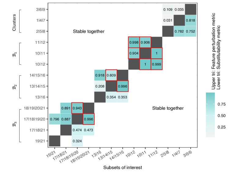
Figure 2. A tile plot for several subsets of interest in the synthetic data. The lower (and upper) triangular matrix in the tile plot displays $\tau(\widebar{S},\widetilde{S};\mathfrak{S})$ values (and $\nabla\tau(\widebar{S},\widetilde{S};\mathfrak{S})$ values) for subsets with $\pi(\widebar{S},\widetilde{S})<0.7$. Blank entries indicate subset pairs that is stable together. The entries highlighted with red frames correspond to pairs that have both large $\tau$ and $\nabla\tau$ values.

In addition to better performance on the metrics described earlier, in highly correlated settings, FSSS can produce multiple stable models, whereas CSS and SS produce only a single model. Specifically, instead of applying greedy FSSS, we repeatedly apply Algorithm 1 using cross-validated parameters $s_{0}=35$ and $\alpha=0.7$ on a single dataset of size $n=600$. This yields $100$ selection sets, denoted by $\mathfrak{S}=\{S_{i}\}_{i=1}^{100}$. Notably, each selection set includes exactly one feature per signal cluster, $|\mathcal{K}_{l}|$ features from blocks $\mathcal{B}_{l}$ ($l=1,2,3$), but no weak signals $X_{22},\dots,X_{26}$ or noise features. In other words, these sets demonstrate a form of “highly correlated” selection consistency within $\{\mathcal{C}_{k}\}_{k\in\mathcal{K}}$ and $\{\mathcal{B}_{l}\}_{l=1}^{3}$, and span similar subspaces through diverse feature combinations, making them equally valid and sparse models for both interpretation and prediction.

We next use our substitutability metrics $\tau$, $\nabla\tau$, and $\triangle\tau$ to identify substitute structures among the $100$ selection sets. In this synthetic setup, we know several subsets of interest and use these to highlight our substitutability metrics. (In the real data analysis in Section 5.2, we will use Algorithm 2 to do a full search for substitute structures). Figure 2 compares several subsets of interest in our synthetic dataset. The lower triangular matrix in the tile plot presents the pairwise $\tau(\widebar{S},\widetilde{S};\mathfrak{S})$. Here, we set $\tau(\widebar{S},\widetilde{S};\mathfrak{S})=0$ if $\widebar{S}$ and $\widetilde{S}$ are together stable (i.e., $\pi(\widebar{S}\cup\widetilde{S})\geq 0.7$), so that $\widebar{S}$ and $\widetilde{S}$ are ignored as potential substitutes. The upper triangular matrix in the tile plot shows pairwise values of $\nabla\tau(\widebar{S},\widetilde{S};\mathfrak{S})$. We observe that the sets $\{1,4,7\}$, $\{2,5,8\}$ and $\{3,6,9\}$ – each selecting one feature per the three clusters – serve as strong substitutes (high $\tau$ values). However, this is largely due to feature perturbation, as indicated by low $\nabla\tau$ values. The block structures $\mathcal{B}_{1}$, $\mathcal{B}_{2}$, and $\mathcal{B}_{3}$, on the other hand, yield subsets that are substitutes that do not arise from feature perturbation structure, with $\tau\geq 0.8$ and $\nabla\tau\geq 0.5$ (see the entries with red frames). Among these sets, we use the metric $\triangle\tau$ to assess whether the substitutability of any pair of sets is primarily driven mostly by substitutability among their subsets. As shown in Figure 3, the substitutability between $\{13,14,15\}$ and $\{14,15,16\}$ essentially reduces to that between $\{13,14,15\}$ and $\{14,16\}$, since $\mathcal{P}_{\{13,14,15\}}y\approx\mathcal{P}_{\{14,16\}}y$. Similarly, the substitutability between $\{17,18,19,20\}$ and $\{18,19,20,21\}$ also degenerate to their respective subsets. Only the subsets in block $\mathcal{B}_{1}$ act as strong, and non-degenerate substitutes.

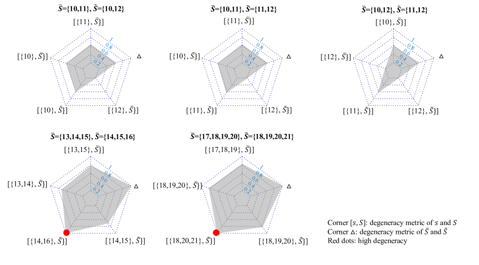
Figure 3. Radar charts of substitutes $(\widebar{S},\widetilde{S})$ with $\tau(\widebar{S},\widetilde{S};\mathfrak{S})\geq 0.8$ and $\nabla\tau(\widebar{S},\widetilde{S};\mathfrak{S})\geq 0.5$ for the synthetic data. The corners $[\widebar{s},\widebar{S}]$ and $[\widetilde{s},\widetilde{S}]$ indicate elements $\widebar{s}\in P(\widebar{S})$ and $\widetilde{s}\in P(\widetilde{S})$ yielding the top two values of $\max_{S\in\mathscr{S}(\widebar{S},\widetilde{S})}\tau(\widebar{s},\widebar{S};S)$ and $\max_{S\in\mathscr{S}(\widebar{S},\widetilde{S})}\tau(\widetilde{s},\widetilde{S};S)$, respectively. The corresponding values are displayed by the shaded region on each corner. The $\triangle$ corner represents $\triangle\tau(\widebar{S},\widetilde{S};\mathfrak{S})$.

5.2. Real data application: gene expression in breast cancer

We consider a publicly available gene expression dataset from the Gene Expression Omnibus with accession code GSE2990 (Sotiriou et al., 2006). The dataset contains microarray measurements from $n=189$ breast cancer tumor samples across 22,283 probes. We filtered out probes with an IQR less than 1.5 and those lacking annotation, resulting in $p=1111$ probes. These remaining expression levels serve as the explanatory variables after centralization. The aim of this analysis is to explore genes potentially associated with breast cancer prognosis. Following the results of Wu et al. (2020), we use the centralized ESR1 gene expression as the response variable $y$, given its established relevance to ER+ breast cancer outcomes.

We use $\ell_{0}$-regression as the base procedure for each stability-based method (greedy FSSS, CSS, and SS). For model selection and assessment, we split the dataset into three folds: subsampling (using $B=200$), feature selection, and coefficient estimation are performed on the first fold (size $n_{\text{fitting}}=143$), validation is performed on the second fold (size $n_{\text{valid}}=16$), and test MSE is assessed using the third fold (size $n_{\text{test}}=30$). Both the stability threshold $\alpha$ and the clustering cutoff height $h$ (for CSS) are chosen based on the validation MSE from the sets $\{0.7,0.75,0.8,0.85,0.9,0.95\}$ and $\{0.1,0.3,0.5\}$, respectively. For each procedure, we fix its corresponding cross-validated parameters $\alpha$ and $h$ (when applicable), and generate $M=50$ different splits of the training data, which are then used to select $M$ different selection sets. For a given split of the data into a training and test set, each procedure’s performance is evaluated based on averaging its test MSE and number of selected features (averaged over the $50$ selection sets). We also compute the output stability of a procedure based on its $50$ selection sets. The analysis above is then repeated over $500$ different splits of the data into training and test set, and the metrics are averaged over these $500$ trials.

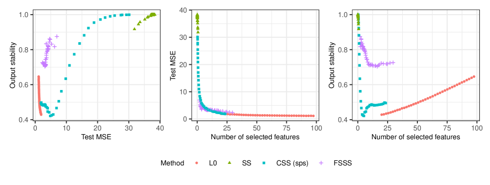
Figure 4. Performance of $\ell_{0}$-regression, SS, sparsity (sps) CSS, and greedy FSSS on the breast cancer gene expression data. The subsampling uses $\ell_{0}$-regression as the base procedure.

Figure 4 compares the test MSE, number of selected features, and output stability across the stability procedures, as well as the base procedure, for different choices of the tuning parameter $s_{0}$. We observe that FSSS is the only method that achieves both high output stability and a nontrivial number of selected features, while effectively stabilizing the base procedure and keeping test MSE low. In contrast, SS seldom selects any feature, whereas CSS cannot achieve low MSE and and high stability simultaneously. Next, we repeatedly apply Algorithm 1 with cross-validated parameters $s_{0}=50$ and stability threshold $\alpha=0.7$ on the entire data. This results in $45$ stable selection sets denoted by $\mathfrak{S}=\{S_{i}\}_{i=1}^{45}$. All selection sets have stability $\pi\in[0.7,0.765]$, and they appear to be scientifically meaningful. As an example, one selection set we obtain includes the following six features: ALDH3B2, IGK_3, CEP55, S100A14, ADAMTS5 and SETD8. Among these, CEP55 and SETD8 are strongly associated with breast cancer, with CEP55 linked to higher tumor grade and poor prognosis, and SETD8 promoting proliferation via histone methylation (Sinha, 2019, Huang et al., 2017). Additional selection sets are provided in Appendix C.3.

Figure 5 presents a dendrogram relating highly substitutable features in the union of $45$ selection sets, using the distance measure $1-\tau(\{i\},\{j\};\mathfrak{S})$ for each pair of features $(i,j)$. Since features that form a stable set together are not considered as substitutes, we set the distance to be one for any $i,j$ with $\pi(\{i,j\})<\alpha$. The most substitutable features are the variants of the same gene expression: (CA12_4, CA12_5) and (ALCAM, ALCAM_2). The expression of both genes are known to be closely associated with breast cancer progression and prognosis, with CA12 upregulated in ER+ tumors and associated with favorable outcomes, while decreased ALCAM expression correlates with higher tumor grade and poorer survival (Lee et al., 2023, King et al., 2004).

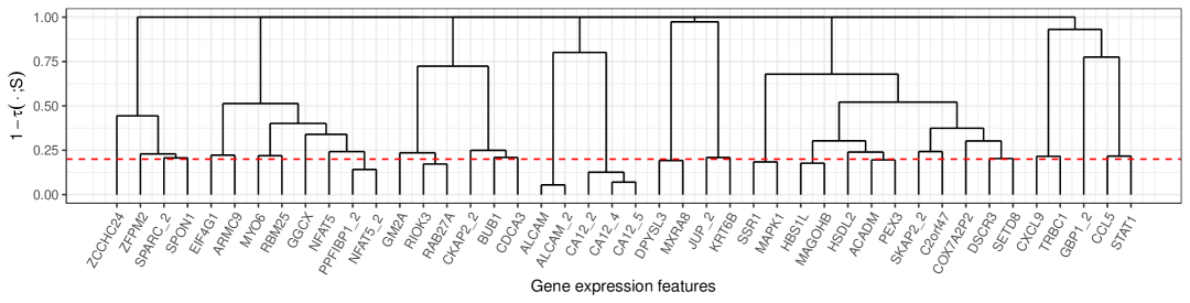
Figure 5. A dendrogram of breast cancer gene expression substitutes $(\{i\},\{j\})$. The distance metric of the dentrogram is $1-\tau(\{i\},\{j\};\mathfrak{S})$ when $\pi(\{i\},\{j\})<0.7$ and 1 otherwise. The red dashed line marks a distance of 0.2.

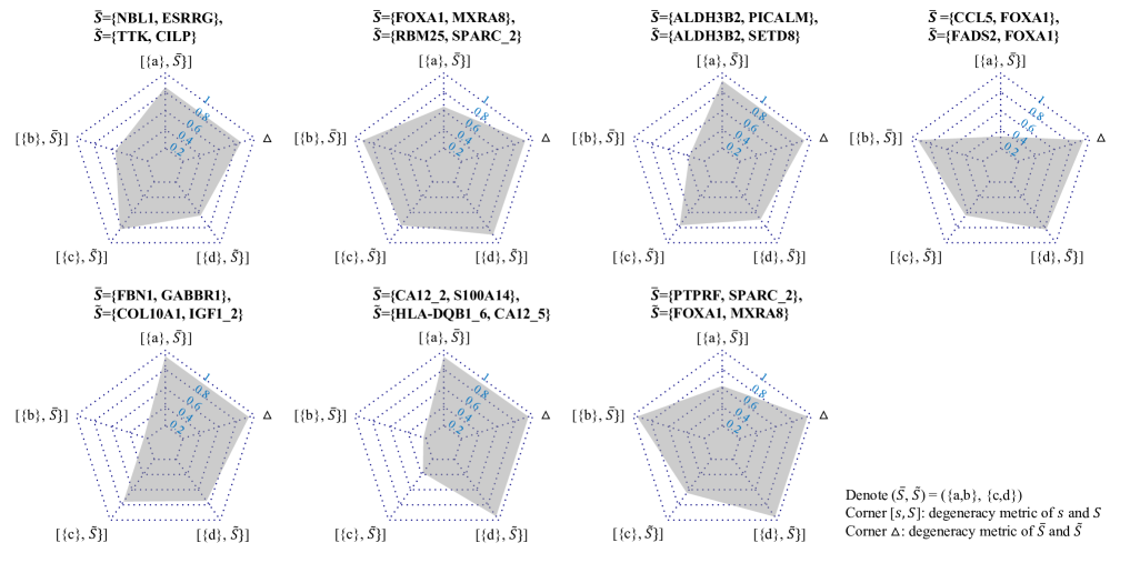
Figure 6. Radar charts of several substitutes identified by Algorithm 2 in the breast cancer dataset. For substitutes in the form of $\{\widebar{S}=(a,b),\widetilde{S}=(c,d)\}$, each corner $[\{i\},\widebar{S}]$ and $[\{j\},\widetilde{S}]$ presents the corresponding $\max_{S\in\mathscr{S}(\widebar{S},\widetilde{S})}\tau(\{i\},\widebar{S};S)$ and $\max_{S\in\mathscr{S}(\widebar{S},\widetilde{S})}\tau(\{j\},\widetilde{S};S)$, respectively, where $i\in\{a,b\}$ and $j\in\{c,d\}$. The $\triangle$ corner presents $\triangle\tau(\widebar{S},\widetilde{S};\mathfrak{S})$.

We now examine more complex subsets returned by Algorithm 2 with $k=2$, $\alpha=0.7$, $\tau_{0}=0.8$, and $\tau_{1}=0.5$. The value of $\tau_{2}$ is set to return the top seven least degenerate substitute pairs. Setting $\tau_{0}=0.8$ helps identify highly substitutable size-2 sets, while $\tau_{1}=0.5$ filters out substitutes caused by “feature perturbation structure.” Figure 6 shows the identified substitutes. We observe that several subsets partially collapse into a single feature – for instance, FOXA1 in the pair (CCL5, FOXA1). Both genes are strongly linked to breast cancer, with FOXA1 specifically known as a favorable prognostic marker in ER+ cases (Thomas et al., 2019, Hurtado et al., 2011). In contrast, pairs like (NBL1, ESRRG) and (TTK, CILP) do not degenerate into smaller subsets. Biologically, NBL1 and ESRRG are linked to tumor-suppressive roles (Nolan et al., 2015, Tiraby et al., 2011), while TTK and CILP are associated with cancer progression and metastasis (King et al., 2018).

6. Discussion

We proposed a subspace framework to quantify false positive/negative errors and stability in highly correlated settings. We also presented an algorithm that leverages our subspace framework to return multiple stable feature sets and described theoretical control on false positive error for this procedure. Further, we proposed metrics to identify substitute structures – namely, features that can be swapped while yielding an equivalent model.

Our work opens several avenues for future research. First, while repeated runs of Algorithm 1 can, in principle, yield all stable models, this process can be inefficient when the number of features is large. It would be interesting to develop more efficient approaches for obtaining all stable models. Second, extending our methodology to generalized additive models with splines — where the response variable depends linearly on unknown spline functions of the predictors – would be of practical interest. Finally, building on the previous point, a general nonlinear version of our framework may be possible by encoding the structure of a prediction model via tangent spaces (i.e., locally linear approximations) of certain manifolds.

7. Acknowledgments

We thank Gemma Moran for insightful conversations. We acknowledge funding from NSF grant DMS-2413074 (Xiaozhu Zhang and Armeen Taeb).

Appendix A Our subspace framework and comparisons to other perspectives

A.1. Connection to model selection over partially ordered sets

There is a strong connection between our proposed subspace framework and the model selection framework proposed in Taeb et al. (2024). We first present the perspective in Taeb et al. (2024), and then describe how our proposed model selection framework is a special case.

Framework in Taeb et al. (2024): Variable selection models are organized as a partially ordered set (poset). The poset is structured hierarchically as shown in Figure 7, starting from its least element (the empty set $\varnothing$), and each model on it is formed by including a new feature to a model at the preceding level. This poset inherits a rank function (formally known as a graded poset) that captures the complexity of a model. In the variable selection poset, the rank of a model $S$ is its cardinality $|S|$, which is also the length of each path from $\varnothing$ to $S$.

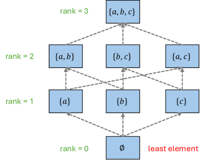
Figure 7. A variable selection poset over features $\{a,b,c\}$.

To assess the similarity between two models $S$ and $\widetilde{S}$, a generic “similarity valuation” metric $\rho(S,\widetilde{S})$ was proposed in Taeb et al. (2024). This metric can take different forms depending on the specific problem domain. Based on this similarity measure, the amount of true positives, false positive error, and false negative error are defined as:

(6) $$\begin{split}\mathrm{TP}(\widehat{S},S^{\star})&:=\rho(\widehat{S},S^{\star}),\\ \mathrm{FPE}(\widehat{S},S^{\star})&:={\rm rank}(\widehat{S})-\rho(\widehat{S},S^{\star}),\\ \mathrm{FNE}(\widehat{S},S^{\star})&:={\rm rank}({S}^{\star})-\rho(\widehat{S},S^{\star}).\end{split}$$

To obtain a model with small false positive error, the poset framework views any selected model $\widehat{S}$ as one that is obtained by following a path that begins at the empty set, and sequentially includes one variable at each level until $\widehat{S}$ is reached. Suppose that the path forming $\widehat{S}$ is given by $(S_{0}=\varnothing,S_{1},\dots,S_{t-1},S_{t}=\widehat{S})$, then the $\mathrm{FPE}(\widehat{S},S^{\star})$ can be written as the telescoping sum

$$\mathrm{FPE}(\widehat{S},S^{\star})=\sum_{i=0}^{t-1}1-\left[\rho(S_{i+1},S^{\star})-\rho(S_{i},S^{\star})\right],$$

where the term $1-[\rho(S_{i},S^{\star})-\rho(S_{i-1},S^{\star})]$ represents the “additional false discovery” incurred by moving from the model $S_{i-1}$ to the model $S_{i}$ on the poset. Based on the telescoping sum decomposition, a greedy algorithm based on subsampling was proposed in Taeb et al. (2024) to control this additional FD term, by guaranteeing the following at each step from $S_{i}$ to $S_{i+1}$:

(7) $$\frac{1}{B}\sum_{\ell=1}^{B}{\rho(S_{i+1},\widehat{S}^{(\ell)})-\rho(S_{i},\widehat{S}^{(\ell)})}\geq\alpha,$$

where $\{\widehat{S}^{(\ell)}\}_{\ell=1}^{B}$ are selection sets obtained from subsampling. The left-hand-side of (7) represent the additional similarity that $S_{i+1}$ exhibits with $\{\widehat{S}^{(\ell)}\}_{\ell=1}^{B}$ relative to $S_{i}$, and is thus a measure of stability associated with the move from model $S_{i}$ to $S_{i+1}$. The quantity $\alpha\in(0,1)$ represents a stability threshold. The algorithm described above is intuitively approximating $1-\left[\rho(S_{i+1},S^{\star})-\rho(S_{i},S^{\star})\right]$ with $\frac{1}{B}\sum_{\ell=1}^{B}{\rho(S_{i+1},\widehat{S}^{(\ell)})-\rho(S_{i},\widehat{S}^{(\ell)})}$.

Our proposed framework: We take $\rho({S},\widetilde{S})={\rm trace}(\mathcal{P}_{{S}}\mathcal{P}_{\widetilde{S}})$, where we use the notation $\mathcal{P}_{S}:=\mathcal{P}_{\mathrm{col}(X_{S})}$. As we describe in Section 2.2 of the main paper, this choice of $\rho$ is motivated by: $(i)$ the subspace $\mathrm{col}(X_{S})$ is a natural and useful representation of $S$ in highly correlated settings; and $(ii)$ motivated by Taeb et al. (2020), the trace inner product of projection matrices onto subspaces is a natural measure of similarity between two subspaces. Note that ${\rm trace}(\mathcal{P}_{{S}}\mathcal{P}_{\widetilde{S}})$ formally qualifies as similarity valuation (as defined in Taeb et al. (2024)) as long as the matrices $X_{S}$ and $X_{\widetilde{S}}$ both consist of linearly independent columns.

With our choice of similarity valuation $\rho$, Definition 1 is a special case of (6). Furthermore, our proposed algorithm FSSS is similar to the algorithm in Taeb et al. (2024) in that it searches for a selection set by growing a path in this poset, starting from the empty set $S_{0}=\varnothing$, and adding one element at a time to reach $S_{i}$. At each step, we require ${\rm trace}((\mathcal{P}_{S_{i}}-\mathcal{P}_{S_{i-1}})\mathcal{P}_{\rm avg})\geq\alpha$, which is a special variate of (7). The final model is denoted by $S_{t}$. As a result, the FPE for $S_{t}$ can be controlled as

$$\begin{split}\mathrm{FPE}(\widehat{S},S^{\star})&=\sum_{i=1}^{t-1}1-\left[{\rm trace}(\mathcal{P}_{S_{i+1}}\mathcal{P}_{S^{\star}})-{\rm trace}(\mathcal{P}_{S_{i}}P_{S^{\star}})\right]\\ &\approx\sum_{i=1}^{t-1}1-\left[{\rm trace}(\mathcal{P}_{S_{i+1}}\mathcal{P}_{\rm avg})-{\rm trace}(\mathcal{P}_{S_{i}}P_{\rm avg})\right]\leq|S_{t}|(1-\alpha),\end{split}$$

where the approximation uses $\mathcal{P}_{\rm avg}$ as an estimate for $\mathcal{P}_{S^{\star}}$. This suggests that $\alpha$-stable models have small false positive error, especially when $\alpha\approx 1$. We provide rigorous false positive error guarantees in Section 4.

A.2. Extension to generalized linear models

Let $X\in\mathbb{R}^{n\times p}$ denote the design matrix, $\beta\in\mathbb{R}^{p}$ denote the coefficient, and $y\in\mathbb{R}^{n}$ denote the response variable. For generalized linear models (GLMs), the conditional expectation of the response is given by $\mathbb{E}[y\mid X]=\mu=g^{-1}(X\beta)$, where $g$ is a link function. Due to the linear component $X\beta$ in GLMs, we can define $\mathrm{TP},\mathrm{FPE},\mathrm{FNE}$ exactly like Definition 1 and stability $\pi$ exactly like Definition 2. Additionally, Algorithm 1 (FSSS) can be applied without any modifications, provided that the base procedures are compatible with the response type – for example, using $\ell_{0}$-penalized logistic regression for binary response $y\in\{0,1\}^{n}$.

However, when assessing substitutability via subspaces, the choice of link function and the type of response variable becomes relevant. In particular, when the model is not linear, $\mathcal{P}_{\mathrm{col}(X_{S})}(y)$ does not represent the component of the response captured by the features in $S$. One can instead estimate $g(\mu)$ – the actual linear combination of $X\beta$ in the GLM framework – and replace all terms involving $\mathcal{P}_{\mathrm{col}(X_{S})}(y)$ in the substitutability metric with $\mathcal{P}_{\mathrm{col}(X_{S})}(g(\widehat{\mu}))$. A possible strategy for estimating $g(\mu_{i})=g(\mathbb{E}[y_{i}\mid X^{(i)}])$ is to use a non-parametric $k$-nearest neighbors (KNN) approach. For the $i$-th observation $X^{(i)}$, we identify its $k$ nearest neighbors, denoted by $N(i)$, and estimate $\widehat{\mu}_{i}$ as $\frac{1}{|N(i)|}\sum_{j\in N(i)}y_{j}$. When the link function is identity, we set $k=1$ so that the estimate of $\mu_{i}$ is simply each $y_{i}$ itself. In contrast, when the link function is the logit function, $k$ must be necessarily greater than 1 in order for $\widehat{\mu}\in(0,1)$, as values of 0 or 1 are not valid under the logistic transformation.

A.3. Regarding our substitutability metric

We address two possible misconceptions about the measure $\tau$ in (3). Clarification (i). For any given $\widebar{S}$, $\widetilde{S}$, $S$, and $a\notin\widebar{S}\cup\widetilde{S}$, it is not always true that $\tau(\widebar{S},\widetilde{S};S)\leq\tau(\widebar{S}\cup\{a\},\widetilde{S}\cup\{a\};S)$. In other words, just because $\widebar{S}$ and $\widetilde{S}$ are strong substitutes, adding $\{a\}$ to both does not necessarily make them strong substitutes as well. This shows that the substitute function ($\tau$) is not always “increasing” for subsets. Here is a counterexample: consider $X_{1}$, $\delta_{2}$, and $\delta_{3}$ as mutually orthogonal, with $|X_{1}|_{2}=1$ and $|\delta_{1}|_{2}=|\delta_{2}|_{2}=\eta_{1}$. Let $X_{2}=X_{1}+\delta_{2}$, $X_{3}=X_{1}+\delta_{3}$, and $y=\delta_{2}+\delta_{3}$. Then, we have $\tau(\{2\},\{3\};\varnothing)=1/(1+\eta_{1}^{2})$, but $\tau(\{1,2\},\{1,3\};\varnothing)=0$.

Clarification (ii). For any set $\widebar{S}$ with $a\notin\widebar{S}$ and $b\notin\widebar{S}$, if $\widebar{S}\cup\{a\}$ and $\widebar{S}\cup\{b\}$ are strong substitutes, $X_{a}$ and $X_{b}$ may not be highly correlated. This means that comparing $\widebar{S}\cup\{a\}$ and $\widebar{S}\cup\{b\}$ is not the same as comparing $\{a\}$ and $\{b\}$. As a counterexample, suppose $X_{1}$ and $X_{2}$ are orthogonal, and let $X_{3}=X_{1}-X_{2}$ and $y=X_{1}+X_{2}$. In this case, we find that $\tau(\{1,3\},\{2,3\};\varnothing)=1$, even though $X_{1}$ and $X_{2}$ are orthogonal and $\tau(\{1\},\{2\};\varnothing)=0$. Another counterexample builds on the idea that the additional feature in each set may be non-predictive. For example, suppose $X_{1}$, $X_{2}$ and $X_{3}$ are mutually orthogonal, and let $y=X_{1}$. In this case, we have $\tau(\{1,2\},\{1,3\};\varnothing)=1$ but $\tau(\{2\},\{3\})=0$.

A.4. Why the proposal in G’Sell et al. (2013) is not suitable for assessing false positive error

First, we define how G’Sell et al. (2013) measure the false positive error. Letting $\widehat{S}$ be a selected set of features and supposing the linear mechanism $y=X\beta^{\star}+\epsilon$ with $X\in\mathbb{R}^{n\times p}$ and $y\in\mathbb{R}^{n}$, G’Sell et al. (2013) project $X\beta^{\star}$ onto the span of the columns of $X$ in $\widehat{S}$ (denoted by $X_{\widehat{S}}$) and obtain a projected mean $X_{\widehat{S}}\widehat{\beta}_{\widehat{S}}$. Then, the false positive error (dubbed false variable selection) associated with the selection set $\widehat{S}$ is measured to be the number of zeros in $\widehat{\beta}_{\widehat{S}}$.

While in some highly correlated settings, this new metric provides more reasonable values than the standard notion, it can yield smaller false positive errors than one might expect. For example, suppose $S^{\star}=\{1\}$, and $\widehat{S}=\{2\}$, where $X_{2}$ is a null feature that is nearly, but not completely, orthogonal to $X_{1}$. Then, a simple calculation shows that $\widehat{\beta}_{\widehat{S}}$ is a scalar that will be nonzero. Hence, G’Sell et al. (2013) would claim that there is no false positive error with this selection set. However, including a null feature instead of a nearly orthogonal signal feature should incur a false positive close to one, which is what our subspace definition outputs.

The shortcoming of G’Sell et al. (2013)’s measure in the previous example arises from its sharp binary decision: namely, that if $\widehat{\beta}_{\widehat{S}}=0$, then we incur a false positive error of one; otherwise, if $\widehat{\beta}_{\widehat{S}}\neq 0$, we incur no false positive errors. As a result, as long as there is any nonzero correlation between $X_{1}$ and $X_{2}$, G’Sell et al. (2013) measures no error. On the other hand, our subspace definition of false positive error varies smoothly depending on the amount of correlation among the features: $\mathrm{FPE}(\widehat{S},S^{\star})=1$ when $X_{1}$ and $X_{2}$ are orthogonal, and $\mathrm{FPE}(\widehat{S},S^{\star})$ decreases gradually as the correlation level increases, with $\mathrm{FPE}(\widehat{S},S^{\star})=0$ when $X_{1}$ and $X_{2}$ are perfectly correlated.

Appendix B Additional theoretical properties of FSSS

Notation: For simplicity, we write the norm $\|x\|_{\ell_{q}}$ as $\|x\|_{q}$. We adopt the notation in Section 3 of the paper, namely that for a vector $w\in\mathbb{R}^{n}$, $\mathcal{P}_{w}=\mathcal{P}_{\mathrm{span}(w)}$ and for any subset $S\subseteq\{1,\dots,p\}$, $\mathcal{P}_{X_{S}}=\mathcal{P}_{\mathrm{col}(X_{S})}$.

This section is organized as follows: Section B.1 presents theoretical properties of $\ell_{0}$-penalized regression as a base procedure under the clustering setup; Section B.2, also under the clustering setup, provides further discussion on the quality terms $\gamma_{\mathcal{W}}$ and $\gamma_{\mathcal{U}}$ introduced in Section 4; and finally, Section B.3 extends our theoretical analysis to setups with complex dependency structures.

B.1. $\ell_{0}$-penalized base procedure

While any feature selection algorithm can serve as the base procedure for FSSS, an $\ell_{0}$-penalized regression is particularly recommended for selecting highly correlated variables. Given a design matrix $X\in\mathbb{R}^{n\times p}$ and a response variable $y\in\mathbb{R}^{n}$, the solution is given by

(8) $$\widehat{\beta}\in\arg\min_{\beta\in\mathbb{R}}\|y-X\beta\|_{2}^{2},\quad{\rm s.t.}\quad\|\beta\|_{0}\leq s_{0}.$$

The following theorem is built on the clustering setup described in Section 4.1.

Theorem 3 (Base procedure).

Suppose $\max_{j\in\mathcal{K}}\mathrm{Corr}(X_{j},\epsilon)\leq\mathcal{O}(\sqrt{\log p/n})$, as well as $\max_{j\in\mathcal{V}}\mathrm{Corr}(\delta_{j},\epsilon)\leq\mathcal{O}(\sqrt{\log p/n})$. Furthermore, assume that $|\mathcal{C}_{k}|=D$ for all $k\in\mathcal{K}$, and

(9) $$\begin{split}\min_{j\in S^{\star}}\left|\beta^{\star}_{j}\right|^{2}>\frac{D\eta_{1}^{2}}{1+\eta_{1}^{2}}\|\beta^{\star}\|_{2}^{2}+\mathcal{O}\left(s_{0}D^{2}\sqrt{\frac{\log p}{n}}\right)(\|\beta^{\star}\|_{1}+\|\epsilon\|_{2})^{2}.\end{split}$$

Then when $s_{0}\geq s^{\star}$,

1. The solution $\widehat{\beta}$ to (8) does not miss any signal groups: there must exist $\widetilde{S}\in\mathcal{S}$ such that $\widetilde{S}\subseteq{\rm supp}(\widehat{\beta})$.

2. When $s_{0}=s^{\star}$, the solution $\widehat{\beta}$ achieves cluster feature selection consistency: ${\rm supp}(\widehat{\beta})\in\mathcal{S}$.

3. When $s_{0}=s^{\star}$ and furthermore

   (10) $$\frac{\eta_{1}^{2}}{1+\eta_{1}^{2}}\|\beta^{\star}\|_{2}^{2}>\mathcal{O}\left(s^{\star}\sqrt{\frac{\log p}{n}}\right)(\|\beta^{\star}\|_{1}+\|\epsilon\|_{2})^{2},$$

   the solution $\widehat{\beta}$ achieves exact feature selection consistency: ${\rm supp}(\widehat{\beta})=S^{\star}$.

We prove Theorem 3 in Section D.2.4. Theorem 3 demonstrates the effectiveness of $\ell_{0}$-regression in the clustering setup. To be specific, under the beta-min condition (9), when $s_{0}\geq s^{\star}$, $\ell_{0}$-regularization manages to select at least one feature per signal group. Under the more restrictive condition $s_{0}=s^{\star}$, exactly one feature is selected per signal group, and no noise clusters can be selected. However, exact feature selection consistency may require a much larger sample size, as indicated by the beta-min condition (10).

Note that Theorem 3 relies on the conditions $\max_{j\in\mathcal{K}}\mathrm{Corr}(X_{j},\epsilon)\leq\mathcal{O}(\sqrt{\log p/n})$, as well as $\max_{j\in\mathcal{V}}\mathrm{Corr}(\delta_{j},\epsilon)\leq\mathcal{O}(\sqrt{\log p/n})$. Under the linear model $y=X\beta^{\star}+\epsilon$, with $\epsilon$ drawn from $\mathcal{N}(0,\sigma^{2}/nI_{n})$, these conditions hold with high probability, as suggested by the concentration inequality $\mathbb{P}\left[\max_{j\in\mathcal{K}}\mathrm{Corr}(X_{j},\epsilon)\leq t,\max_{j\in\mathcal{V}}\mathrm{Corr}(\delta_{j},\epsilon)\leq t\right]\geq 1-ap\exp\{-bnt^{2}\}$ for some $a,b>0$. As a result, and as noted in Remark 3, the $\ell_{0}$-regularized regression is very likely to satisfy the condition (i) in Theorem 1, and hence serves as a good candidate of base procedure for FSSS to achieve promising results.

B.2. Quality of base procedure

Definition 6 characterizes the quality of a base procedure via the terms $\gamma_{\mathcal{W}}$ and $\gamma_{\mathcal{U}}$. In this section, we analyze the behavior of these quantities.

Regarding the term $\gamma_{\mathcal{W}}$: The quality term appeared in Theorem 1. Recall that the collection of all “noise directions” is defined as $\mathcal{W}:=\{\delta_{j}:j\in\mathcal{V}\}\cup\bigcup_{j\in\mathcal{K}\cap N^{\star}}\{X_{j}\}$. We also define the index set $W:=\mathcal{V}\cup(\mathcal{K}\cap N^{\star})$, and associate each $j\in W$ with a direction $w_{j}$, where $w_{j}=\delta_{j}$ for $j\in\mathcal{V}$ and $w_{j}=X_{j}$ for $j\in\mathcal{K}\cap N^{\star}$. That is, we write $\mathcal{W}=\{w_{j}\}_{j\in W}$. We further denote $w_{j}=X_{j}$ for any $j\in[p]\setminus W$. With these notations in place, we introduce two standard assumptions that are commonly used in the study of stability-based methods, to enable a more refined analysis of $\gamma_{\mathcal{W}}$.

Assumption 1 (Better than random guessing).

For all subsamples $\ell\in\{1,\dots,B\}$,

$$\frac{\sum_{j\in W}\mathbb{E}\left[{\rm trace}(\mathcal{P}_{w_{j}}\mathcal{P}_{X_{\widehat{S}^{(\ell)}}})\right]}{p-s^{\star}}\leq\frac{\sum_{j\in[p]\setminus W}\mathbb{E}\left[{\rm trace}(\mathcal{P}_{w_{j}}\mathcal{P}_{X_{\widehat{S}^{(\ell)}}})\right]}{s^{\star}}.$$

Assumption 2 (Exchangeability).

The noise directions are exchangeable in the following sense: for all $j\in W$, $\inf_{T\in\mathscr{T}}\mathbb{E}\left[{\rm trace}(\mathcal{P}_{w_{j}}\mathcal{P}_{X_{\widehat{S}(T)}})\right]\equiv l,$ where $\widehat{S}(T)$ is the selection set of the base procedure on subsample $T$.

Informally, Assumption 1 states that the normalized power of the base procedure on signal directions exceeds its normalized false discovery rate on noise directions. Assumption 2, on the other hand, assumes that the minimum false discoveries made by the base procedure is uniformly distributed across all the noise directions. Remark 5 provides insights into scenarios in which these assumptions are likely to hold.

Under the two assumptions above, Proposition 4 below establishes an upper bound on the quality term $\sum_{j\in W}\sup_{T\in\mathscr{T}}\mathbb{E}\left[{\rm trace}(\mathcal{P}_{w_{j}}\mathcal{P}_{X_{\widehat{S}(T)}})\right]$, which serves as a proxy for $p\gamma_{\mathcal{W}}$. By comparing these two expressions, we find that $\gamma_{\mathcal{W}}$ is approximately $s_{0}/p+1/p\sum_{j\in[p]}r_{j}+\mathcal{O}(s_{0}\sqrt{\log p/n})$. In particular, under the special case described in Remark 5, this quantity simplifies exactly to $s_{0}/p$.

Proposition 4.

Let $r_{j}=\sup_{T\in\mathscr{T}}\mathbb{E}\left[{\rm trace}(\mathcal{P}_{w_{j}}\mathcal{P}_{X_{\widehat{S}(T)}})\right]-l$ for any $j\in[p]$. Under the Assumptions 1 – 2, we have

$$\begin{split}\sum_{j\in W}\sup_{T\in\mathscr{T}}\mathbb{E}\left[{\rm trace}(\mathcal{P}_{w_{j}}\mathcal{P}_{X_{\widehat{S}(T)}})\right]\leq s_{0}+\sum_{j\in[p]}r_{j}+\mathcal{O}\left(s_{0}p\sqrt{\frac{\log p}{n}}\right),\end{split}$$

and

$$\begin{split}&\sum_{j\in W}\sup_{T\in\mathscr{T}}\mathbb{E}\left[{\rm trace}(\mathcal{P}_{w_{j}}\mathcal{P}_{X_{\widehat{S}(T)}})\right]^{2}\leq\frac{s_{0}^{2}}{p}+\sum_{j\in[p]}\left[r_{j}^{2}+\frac{2s_{0}}{p}{r_{j}}\right]+\mathcal{O}\left(s_{0}^{2}p\sqrt{\frac{\log p}{n}}\right).\end{split}$$

Before moving on to the second perspective, we present an immediate corollary of Proposition 4. As shown in Remark 5, the resulting FPE upper bound simplifies to that of stability selection, up to an additive constant factor related to the length of the perturbation directions.

Corollary 5.

Let $r_{j}=\sup_{T\in\mathscr{T}}\mathbb{E}\left[{\rm trace}(\mathcal{P}_{w_{j}}\mathcal{P}_{X_{\widehat{S}(T)}})\right]-l$ for any $j\in[p]$. Under the conditions of Theorem 1 and Assumptions 1 – 2, for every $S$ returned by Algorithm 1,

$$\begin{split}\mathbb{E}\left[\mathrm{FPE}(S,S^{\star})\right]\leq\frac{1}{2\alpha-1}\left[\frac{s_{0}^{2}}{p}+\sum_{j\in[p]}\left(r_{j}^{2}+\frac{2s_{0}}{p}r_{j}\right)\right]+f(\eta_{1})+\mathcal{O}\left(s_{0}^{2}p\sqrt{\frac{\log p}{n}}\right),\end{split}$$

where $f(\eta_{1})=[2(s_{0}+\sum_{j\in[p]}r_{j})\sqrt{\eta_{1}^{2}/(1+\eta_{1}^{2})}+4p\eta_{1}^{2}/(1+\eta_{1}^{2})]/(2\alpha-1)+s_{0}\eta_{1}^{2}/(1+\eta_{1}^{2}).$

Both Proposition 4 and Corollary 5 are proved in Section D.2.5.

Regarding the term $\gamma_{\mathcal{U}}$: This term appears in Theorem 2. Recall that $\mathcal{U}:=\bigcup_{k\in S^{\star}}\{\delta_{j}-\delta_{l}:j\neq l\in\mathcal{V}_{k}\}\cup\bigcup_{k\in\mathcal{K}\cap S^{\star}}\{\delta_{j}:j\in\mathcal{V}_{k}\}\cup\bigcup_{k\in\mathcal{K}\cap N^{\star}}\{X_{j}:j\in\mathcal{C}_{k}\}$. Our heuristic approximation on $\gamma_{\mathcal{U}}$ is based on the following idea: when the sample size $n$ is sufficiently large, both the full data set and any subsample would approximate an idealized setting, in which the directions of representative features, perturbations, and noise are exactly orthogonal. Therefore, analyzing the behavior of $\gamma_{\mathcal{U}}$ under this idealized setup provides valuable insight into its asymptotic behavior.

In order to construct such an idealized setup, we distinguish between two key components of the FSSS procedure: index estimation and subspace estimation. For index estimation, we apply the base procedure to disjoint pairs of subsamples $\mathscr{T}:=\{T^{(2\ell-1)},T^{(2\ell)}\}_{\ell=1}^{B/2}$, where $T^{(2\ell-1)}\cap T^{(2\ell)}=\varnothing$, yielding $B$ estimates $\{\widehat{S}^{(2\ell-1)},\widehat{S}^{(2\ell)}\}_{\ell=1}^{B/2}$. For subspace estimation, we compute the average projection matrix $\mathcal{P}_{\rm avg}=\frac{1}{B}\sum_{\ell=1}^{B}\mathcal{P}_{\widehat{S}^{(\ell)}}$ based on a design matrix restricted to a subset of observations $\mathscr{D}\subseteq\{1,\dots,n\}$. Importantly, the sets $\{T^{(2\ell-1)},T^{(2\ell)}\}_{\ell=1}^{B/2}$ need not be complementary subsamples of equal size, and the evaluation set $\mathscr{D}$ need not coincide with the full dataset. No intrinsic relationship is required between the subsampling sets used for index estimation and the data used for subspace estimation.

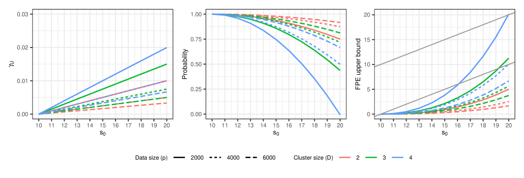
Figure 8. A numerical experiment illustrating the behavior of $\gamma_{\mathcal{U}}$ and its related quantities, with $\alpha_{0}=0.1$, $\eta_{1}=0.01$, $s^{\star}=10$, and $p=2000$. Left panel: $\gamma_{\mathcal{U}}$ values for different $s_{0}$. Middle panel: the probability $1-(s^{\star}\binom{D-1}{2}+p-s^{\star})\cdot\gamma_{\mathcal{U}}^{2}/(1-2\alpha_{0})$ for different $s_{0}$. Right panel: FPE upper bound for different $s_{0}$, where the gray lines indicate the upper bound and lower bound for $\ell_{0}$-base procedures respectively.

Building on this generalization, we now assume that the subspace estimation indices $\mathscr{D}$ and the index estimation indices $\mathscr{T}$ form a partition of $\{1,\dots,n\}$. Within each partition, we further assume that the components $X_{\mathcal{K}}$, $\delta_{\mathcal{V}}$ and $\epsilon$ are perfectly orthogonal; that is, $Z_{i}\perp Z_{j}$ for all $Z_{i}\neq Z_{j}\in X_{\mathcal{K}}\cup\delta_{\mathcal{V}}\cup\{\epsilon\}$. Additionally, we assume that each cluster has size $D>1$. In this setting,

(11) $$\gamma_{\mathcal{U}}=\max\left\{\frac{s_{0}-s^{\star}}{p-s^{\star}},\quad 1-\prod_{i=1}^{D-1}\frac{p-s_{0}-i}{p-s^{\star}-i}\right\},$$

which is about $s_{0}/p$ when $s_{0}$ and $p$ are sufficiently large (see Section D.2.6 for a proof). Figure 8 shows a numerical experiment examining the behavior of $\gamma_{\mathcal{U}}$, the probability of $\mathfrak{S}\subseteq\mathcal{S}$, and the FPE upper bound. We observe a meaningful region where FSSS achieves uniformly lower FPE upper bounds than the base procedure, highlighting the benefits of subsampling.

As a final remark, we point out that this idealized setting can also be applied to $\gamma_{\mathcal{W}}$ analysis. Remark 5 presents a special scenario, in the same spirit of the perfectly orthogonal setting, under which the Assumptions 1 – 2 hold.

Remark 5.

Consider such a special example: (i) the subspace estimation indices $\mathscr{D}$ and the index estimation indices $\mathscr{T}$ are a partition of $\{1,\dots,n\}$; (ii) For each partition, $X_{\mathcal{K}}$, $\delta_{\mathcal{V}}$ and $\epsilon$ are perfectly orthogonal to each other. In this case, the RHS of Assumption 1 attains 1, which is a trivial upper bound of the LHS.

On top of the two conditions above, we further require that all non-singleton clusters are signal clusters (meaning that $\left\{k\in\mathcal{K}:|\mathcal{C}_{k}|\neq 1\right\}\subseteq S^{\star}$). In this case, for $\ell_{0}$-base procedure, $\sup_{T\in\mathscr{T}}\mathbb{E}\left[{\rm trace}(\mathcal{P}_{w_{j}}\mathcal{P}_{X_{\widehat{S}(T)}})\right]=\inf_{T\in\mathscr{T}}\mathbb{E}\left[{\rm trace}(\mathcal{P}_{w_{j}}\mathcal{P}_{X_{\widehat{S}(T)}})\right]\equiv(s_{0}-s^{\star})/(p-s^{\star})$ for any $j\in W$. Hence,

$$\mathbb{E}\left[\mathrm{FPE}(S,S^{\star})\right]\leq\frac{1}{2\alpha-1}\left[\frac{s_{0}^{2}}{p}+2s_{0}\sqrt{\frac{\eta_{1}^{2}}{1+\eta_{1}^{2}}}+\frac{4p\eta_{1}^{2}}{1+\eta_{1}^{2}}\right]+\frac{s_{0}\eta_{1}^{2}}{1+\eta_{1}^{2}}.$$

Figure 9 presents FPE upper bounds for this special example, which are uniformly lower than $s_{0}-s^{\star}$, the lower bound for FPE incurred by $\ell_{0}$-base procedure.

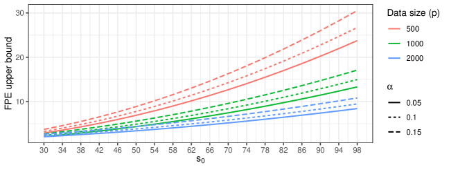
Figure 9. A numerical experiment for the FPE upper bound under Assumptions 1 and 2, with $\alpha=0.9$, $\eta_{1}=0.01$, and $s^{\star}=10$.

B.3. Beyond clustering: the complex dependency setup

We consider a design matrix composed of block structures. Let $\mathcal{K}$ be the index set of block parents. For any $k\in\mathcal{K}$, we assume for simplicity that $X_{k}$ is normalized so that $\|X_{k}\|_{2}=1$. Suppose that the child of $\mathcal{K}$ is given by $X_{c}=\sum_{j\in\mathcal{K}}X_{j}+\delta$, where $\delta$ is a perturbation with $\|\delta_{j}\|_{2}=\eta_{1}\ll 1$. The entire block is denoted by $\mathcal{B}:=\mathcal{K}\cup\{c\}$. Additionally, there are individual features indexed by $\mathcal{I}$, where for any $k\in\mathcal{I}$, $X_{k}$ is normalized so that $\|X_{k}\|_{2}=1$. We further assume that all $X_{k}$, $k\in\mathcal{K}\cup\mathcal{I}$, and the perturbation $\delta$ are nearly orthogonal; that is, for all $k\neq k^{\prime}\in\mathcal{K}\cup\mathcal{I}$, the correlation $|\cos\langle X_{k},X_{k^{\prime}}\rangle|$ and $\cos\langle X_{k},\delta\rangle|$ are upper bounded by $\mathcal{O}(\sqrt{\log p/n})$.

The response variable is generated from block parents and individual features: $y=\sum_{k\in\mathcal{K}\cup\mathcal{I}}X_{k}\beta^{\star}_{k}+\epsilon.$ Here $\epsilon\in\mathbb{R}^{n}$ is a random vector with independent and identically distributed entries. We define the signal block parents as $S^{\star}_{\mathcal{B}}:=\{k\in\mathcal{K}:\beta^{\star}_{k}\neq 0\}$, the noise block parents as $N^{\star}_{\mathcal{B}}:=\{k\in\mathcal{K}:\beta^{\star}_{k}=0\}$, the signal individual parents as $S^{\star}_{\mathcal{I}}:=\{k\in\mathcal{I}:\beta^{\star}_{k}\neq 0\}$, and the noise individual parents as $N^{\star}_{\mathcal{I}}:=\{k\in\mathcal{I}:\beta^{\star}_{k}=0\}$. Moreover, let $K:=|\mathcal{K}|$, $S^{\star}:=S^{\star}_{\mathcal{B}}\cup S^{\star}_{\mathcal{I}}$, and $s^{\star}:=\left|S^{\star}\right|$.

Finally, note that since $\eta_{1}\ll 1$, when $N^{\star}_{\mathcal{B}}=\varnothing$, models that select $K$ features from $\mathcal{K}$ are nearly indistinguishable. In other words, models selecting all parents in $\mathcal{B}$, and models selecting any $K-1$ parents and the child in $\mathcal{B}$ span similar subspaces. As a result, targeting the signal set $S^{\star}$ is not meaningful. Instead, we define a class of “block consistency models”:

$$\mathcal{S}_{0}:=\left\{{\rm supp}(\beta):\beta\in\mathbb{R}^{p};\ \left|{\rm supp}(\beta)\cap\mathcal{B}\right|=K;\ \beta_{j}\neq 0\ \forall j\in S^{\star}_{\mathcal{I}};\ \beta_{j}=0\ \forall j\in N^{\star}_{\mathcal{I}}\right\}.$$

Note that all models in $\mathcal{S}_{0}$ span similar subspaces when $N^{\star}_{\mathcal{B}}=\varnothing$. We further denote $\mathcal{S}_{1}:=\left\{S^{\star}\right\},$ and

$$\mathcal{S}:=\left\{S:S\in\mathcal{S}_{0}\text{ if $N^{\star}_{\mathcal{B}}=\varnothing$};\ S\in\mathcal{S}_{1}\text{ if $N^{\star}_{\mathcal{B}}\neq\varnothing$}\right\}.$$

We first present the properties of $\ell_{0}$-penalized base procedure (8) in the complex dependency setup. Specifically, under a certain beta-min condition, when $s_{0}\geq s^{\star}$, the $\ell_{0}$-base procedure does not miss any signal directions. When $s_{0}=s^{\star}$, the “block selection consistency” is achieved. We proof Theorem 6 in Section D.3.2.

Theorem 6 (Base procedure).

Suppose that $\max_{j\in\mathcal{K\cup\mathcal{I}}}\mathrm{Corr}(X_{j},\epsilon)\leq\mathcal{O}(\sqrt{\log p/n})$ and $\mathrm{Corr}(\delta,\epsilon)\leq\mathcal{O}(\sqrt{\log p/n})$. Furthermore, assume that

(12) $$\begin{split}&\min\left\{\frac{\min_{j\neq k\in S^{\star}_{\mathcal{B}}}|\beta^{\star}_{j}-\beta^{\star}_{k}|^{2}+2\eta_{1}^{2}\min_{j\in S^{\star}_{\mathcal{B}}}|\beta^{\star}_{j}|^{2}}{1+K+(1-K)\mathds{1}_{\{N^{\star}_{\mathcal{B}}=\varnothing\}}+\eta_{1}^{2}},\ \frac{(\eta_{1}^{2}+1)\min_{j\in S^{\star}_{\mathcal{B}}}|\beta^{\star}_{j}|^{2}\mathds{1}_{\{N^{\star}_{\mathcal{B}}\neq\varnothing\}}}{K+\eta_{1}^{2}},\ \min_{j\in S^{\star}_{\mathcal{I}}}|\beta_{j}^{\star}|^{2}\right\}\\ >{}&\frac{\eta_{1}^{2}}{1+\eta_{1}^{2}}\|\beta^{\star}\|_{2}^{2}+\mathcal{O}\left((s_{0}+K)\sqrt{\frac{\log p}{n}}\right)(\|\beta^{\star}\|_{1}+\|\epsilon\|_{2})^{2},\end{split}$$

and additionally

$$\min_{j\in S^{\star}_{\mathcal{B}}}|\beta^{\star}_{j}|^{2}>\mathcal{O}\left(s_{0}\sqrt{\frac{\log p}{n}}\right)\left(\|\beta^{\star}\|_{1}+\|\epsilon\|_{2}\right)^{2}.$$

Then when $s_{0}\geq s^{\star}$,

1. The solution $\widehat{\beta}$ to (8) does not miss any signals. That is, there must exist $\widetilde{S}\in\mathcal{S}_{0}\cup\mathcal{S}_{1}$ such that $\widetilde{S}\subseteq{\rm supp}(\widehat{\beta})$.

2. When $s_{0}=s^{\star}$, the solution $\widehat{\beta}$ achieves block feature selection consistency: ${\rm supp}(\widehat{\beta})\in\mathcal{S}$.

Analogously to the clustering setup, the following theorem demonstrates how FSSS, coupleding with an appropriate base procedure, returns models in $\mathcal{S}$ even if the base procedure chooses many noise or redundant or noise features. Denote the quality of base procedures by

$$\gamma:=\max_{u\in\mathcal{U}}\max_{T\in\mathscr{T}}\mathbb{E}\left[{\rm trace}(\mathcal{P}_{u}\mathcal{P}_{X_{\widehat{S}(T)}})\right],$$

where $\mathscr{T}$ is the collection of subsample indices; additionally, the “undesired direction” is given by $\mathcal{U}:=\{\delta\}\cup\bigcup_{j\in N^{\star}_{\mathcal{I}}}\{X_{j}\}$ if $N^{\star}_{\mathcal{B}}=\varnothing$, and $\mathcal{U}:=\{X_{c}\}\cup\bigcup_{N^{\star}_{\mathcal{B}}\cup N^{\star}_{\mathcal{I}}}\{X_{j}\}$ otherwise.

Theorem 7 (Subsampling consistency).

Suppose that

1. The base procedure does not miss any signal: for any $\ell\in\{1,\dots,B\}$, there must exist $S\in\mathcal{S}_{0}\cup\mathcal{S}_{1}$ such that $S\subseteq\widehat{S}^{(\ell)}$.

2. $\max\left\{\frac{\eta_{1}^{2}}{1+\eta_{1}^{2}},\ \frac{|S^{\star}_{\mathcal{B}}|}{K+\eta_{1}^{2}}\right\}+\mathcal{O}(s^{\star}(K+s^{\star})\sqrt{\frac{\log p}{n}})<\frac{1}{2}$, and $s^{\star}\leq(\frac{n}{\log p})^{1/8}$.

3. $K^{2}\sqrt{\log p/n}\rightarrow 0$ as $K,p,n\rightarrow\infty$.

Then for any $\alpha_{0}\in(0,1/2)$, with the threshold

$$f_{1}(\eta_{1})-\alpha_{0}+\mathcal{O}\left(s^{\star}\sqrt{\frac{\log p}{n}}\right)\leq\alpha\leq f_{2}(s^{\star},\eta_{1},s_{0})+\mathcal{O}\left(s^{\star}(s_{0}+B)\sqrt{\frac{\log p}{n}}\right),$$

where $f_{1}(\eta_{1}):=1+20\sqrt{\eta_{1}^{2}/(1+\eta_{1}^{2})}+8\eta_{1}^{2}/(1+\eta_{1}^{2}),$ and $f_{2}(s^{\star},\eta_{1},s_{0}):=1-(3(s^{\star})^{2}+2s^{\star}s_{0})\sqrt{\eta_{1}^{2}/(1+\eta_{1}^{2})}+(3s^{\star}+s_{0})\eta_{1}^{2}/(1+\eta_{1}^{2})+\left(\eta_{1}^{2}/(1+\eta_{1}^{2})\right)^{3/2},$ we have $\mathfrak{S}\subseteq\mathcal{S}$ with probability $1-\left(p-s^{\star}\right)\cdot\gamma^{2}/(1-2\alpha_{0})$.

We proof Theorem 7 in Section D.3.3. Theorem 7 reveals that, under certain conditions, the subspaces spanned by FSSS selection sets closely resemble the oracle subspace ${\rm span}(X_{S^{\star}})$ with high probability. Consequently, false discovery can be immediately controlled, as established in Corollary 8.

Corollary 8.

Under the assumptions of Theorem 7, we further assume that the FSSS algorithm stops before it selects $s_{0}$ features. Then, every FSSS selection set $S$ satisfies the FPE bound:

$$\begin{split}\mathbb{E}\left[\mathrm{FPE}(S,S^{\star})\right]&\leq\frac{\eta_{1}^{2}}{1+\eta_{1}^{2}}\left[1-\left(p-s^{\star}\right)\cdot\gamma^{2}/(1-2\alpha_{0})\right]+\mathcal{O}\left((s^{\star})^{2}\sqrt{\frac{\log p}{n}}\right)\\ &\quad+s_{0}\left(p-s^{\star}\right)\cdot\gamma^{2}/(1-2\alpha_{0}).\end{split}$$

We proof Corollary 8 in Section D.3.4.

Remark 6.

We study the behavior of $\gamma$ in Theorem 7 throught a very special case. Suppose that the subspace estimation indices $\mathscr{D}$ and the index estimation indices $\mathscr{T}$ are a partition of $\{1,\dots,n\}$. For each partition, $\mathcal{K}$, $\{\delta\}$, $\mathcal{I}$ and $\epsilon$ are perfectly orthogonal: $Z_{i}\perp Z_{j}$ for all $Z_{i}\neq Z_{j}\in X_{\mathcal{K}}\cup\{\delta\}\cup\mathcal{I}\cup\{\epsilon\}$. In this case,

$$\begin{split}\gamma=&\frac{s_{0}-s^{\star}}{p-s^{\star}}\\ &+\max\left\{\sum_{m=0}^{|N^{\star}_{\mathcal{B}}|}\frac{(|S^{\star}_{\mathcal{B}}|+m)}{K+\eta_{1}^{2}}\frac{\binom{|N^{\star}_{\mathcal{B}}|}{m}\binom{p-s^{\star}-|N^{\star}_{\mathcal{B}}|-1}{s_{0}-s^{\star}-m}}{\binom{p-s^{\star}}{s_{0}-s^{\star}}},\sum_{m=0}^{|N^{\star}_{\mathcal{B}}|-1}\frac{1}{|N^{\star}_{\mathcal{B}}|-m+\eta_{1}^{2}}\frac{\binom{|N^{\star}_{\mathcal{B}}|-1}{m}\binom{p-s^{\star}-|N^{\star}_{\mathcal{B}}|-1}{s_{0}-s^{\star}-m}}{\binom{p-s^{\star}}{s_{0}-s^{\star}}}\right\}.\end{split}$$

See Section D.3.5 for a proof. Figure 10 shows a numerical experiment of $\gamma$, the probability of $\mathfrak{S}\subseteq\mathcal{S}$, and the FPE upper bound. We observe a meaningful region where FSSS achieves uniformly lower FPE upper bounds than the base procedure, attributable to the benefits of subsampling.

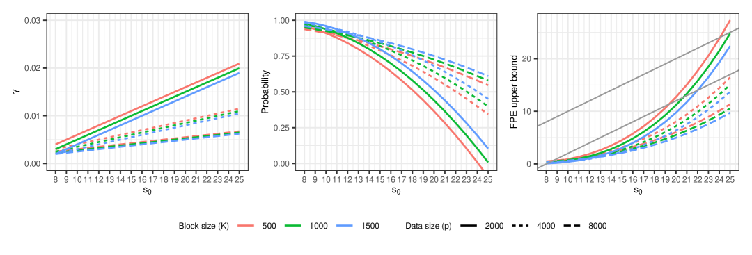
Figure 10. A numerical experiment illustrating the behavior of $\gamma$ and its related quantities in Theorem 7, with $\alpha_{0}=0.1$, $\eta_{1}=0.01$, $|S^{\star}_{\mathcal{I}}|=5$, and $|N^{\star}_{\mathcal{B}}|=\lfloor 0.998K\rfloor$. Left panel: $\gamma$ values for different $s_{0}$. Middle panel: the probability $1-(p-s^{\star})\cdot\gamma^{2}/(1-2\alpha_{0})$ for different $s_{0}$. Right panel: the FPE upper bounds for different $s_{0}$, where the gray lines indicate the upper bound and lower bound for $\ell_{0}$-base procedures respectively.

Appendix C Simulation and data application details

C.1. Setup of Figure 1

Figure 1 presents stability paths of each individual feature on a synthetic dataset $(X\in\mathbb{R}^{n\times p},y\in\mathbb{R}^{n})$. This dataset contains $n=100$ observations and $p=82$ features, organized into 8 cluster blocks, 2 dependency blocks, and 50 individual features. Specifically, for each cluster $\mathcal{C}_{k}=\{k,k+1,k+2\}$ where $k\in\{1,4,7,10,13,16,19,22\}$, the representative feature is generated as $X_{k}\overset{iid}{\sim}\mathcal{N}(0,I_{n})$. The proxies are defined as $X_{j}=X_{k}+\delta_{j}$ for $j\in\{k+1,j+2\}$, where the perturbation directions follow $\delta_{j}\overset{iid}{\sim}\mathcal{N}(0,0.2^{2}I_{n})$. For the first dependency block $\mathcal{B}_{1}=\{25,26,27,28\}$, the parents $X_{25}$ and $X_{26}$ are iid drawn from $\mathcal{N}(0,I_{n})$. Their first child is defined as $X_{27}=X_{25}+X_{26}+\delta_{27}$, and the second as $X_{28}=X_{25}-X_{26}+\delta_{28}$, where the perturbations follows $\delta_{j}\overset{iid}{\sim}\mathcal{N}(0,0.2^{2})$, $j\in\{27,28\}$. The second dependency block $\mathcal{B}_{2}=\{29,30,31,32\}$ is generated in the same way as $\mathcal{B}_{1}$, with $X_{29}$ and $X_{30}$ as the parents, and $X_{31}$ and $X_{32}$ as the children. The remaining 50 individual features are iid drawn from $\mathcal{N}(0,I_{n})$. All representative features, perturbation directions, and individual features are independently generated.

We assign coefficients one to all representative features, while setting the coefficients of their proxies as zero. For each dependency block, the two parent features are assigned coefficients of 1.5 and 1, respectively, whereas the child features receive zero coefficients. All remaining individual features are treated as noise with zero coefficients. Letting $\beta^{\star}$ denote the coefficient vector, the response variable is generated as $y=X\beta^{\star}+\epsilon$ where $\epsilon\overset{iid}{\sim}\mathcal{N}(0,0.2^{2}I_{n})$. Under this setup, the “signal” features in the legend of Figure 1 refer to all representative features in clusters, and all parents features from dependency blocks. The “correlated signal” refers to the cluster proxies and the children in dependency blocks. Finally, the “noise” features refer to those individual features with zero coefficients.

We clarify the quantities computed for each panel in Figure 1. We perform subsampling using $\ell_{0}$-penalized regression as the base procedure, with a total of 100 subsamples. The tuning parameter is the number of features selected in each subsample. In the left panel, corresponding to standard stability selection, the stability value for each feature refers to its selection proportion across the subsamples. In the middle panel, corresponding to cluster stability selection, the stability value refers to the selection proportion of the cluster to which each feature belongs. Clusters are determined using hierarchical clustering with a distance metric defined as $1-\mathrm{cor}(X_{j},X_{k})$ for any two features $X_{j}$ and $X_{k}$, and a cutoff height of 0.2. In the right panel, under our proposed subspace framework, the stability of each feature is measured by the subspace-based quantity $\pi(X_{j})$.

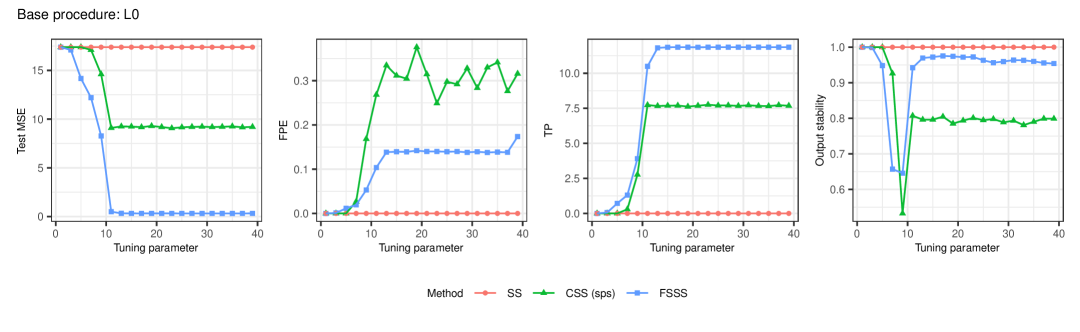
Figure 11. Performance of SS, sparsity (sps) CSS, and FSSS on the dataset of Figure 1 with $\alpha=0.8$. The subsampling uses $\ell_{0}$-regression as the base procedure, and takes $B=100$ subsamples. The tuning parameter is the number of selected features for each subsample.

Lastly, we evaluate the performance of stability selection, sparse cluster stability selection, and FSSS on this dataset with $\alpha=0.8$. Specifically, we apply feature selection and coefficient estimation on this dataset, and report the test MSE, FPE, TP, and output stability using a separate test set drawn from the same distribution. We repeat this procedure $M=50$ times. As shown in Figure 11, stability selection hardly makes any selection, and FSSS uniformly outperforms CSS in terms of test MSE, FPE, TP, and output stability.

C.2. More on the simulations

In Section 5, we compared the performance of different methods across tuning parameters $s_{0}\in\{2,3,\dots,41\}$. Figure 12 and 13 display the evaluation metrics for all $s_{0}$.

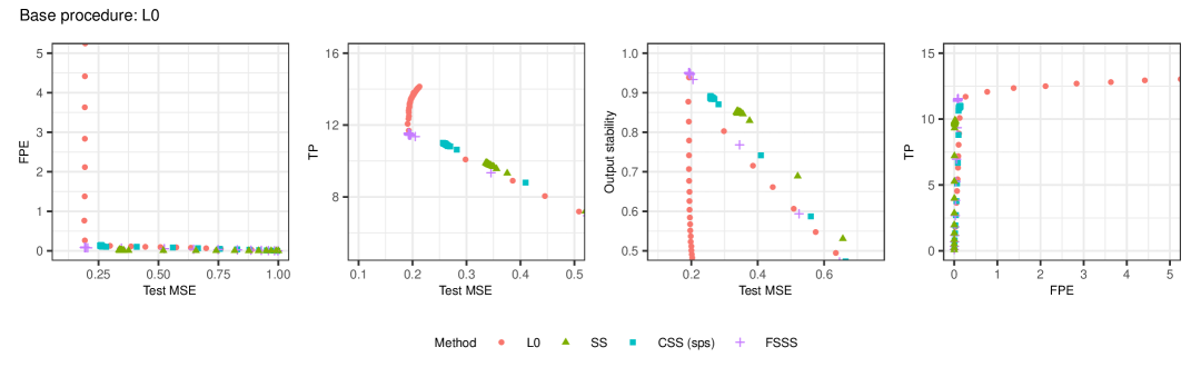
Figure 12. Performance of SS, sparsity (sps) CSS, and FSSS on synthetic datasets. The subsampling uses $\ell_{0}$-regression as the base procedure, and takes $B=200$ subsamples. The tuning parameter is the number of selected features for base procedures.

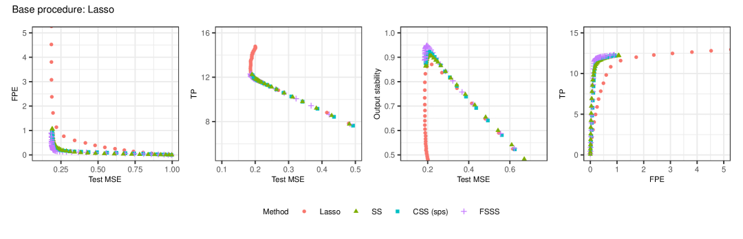
Figure 13. Performance of SS, sparsity (sps) CSS, and FSSS on synthetic datasets. The subsampling uses Lasso as the base procedure, and takes $B=200$ subsamples. The tuning parameter is the number of selected features for base procedures.

C.3. More on the breast cancer dataset

All 45 selection sets in $\mathfrak{S}$ are listed in Table 2.

ALDH3B2, IGK_3, CEP55, S100A14, ADAMTS5, SETD8	MBNL1, AR_2, ZCCHC24, PPFIBP1_2, S100A14
SSR1, BCL2, COL11A1, ID4, HLA-DQB1_6	ALDH3B2, ESR1, IGF1, PTPRC, PICALM
MYB, COL10A1, IGF1_2, HOMER1, NFAT5_2	TOP2A, CD24, WWP1, C1orf115, COL11A1_2
CDC20, MYO6, TRBC1_2, SKAP2_2, S100A14	DPYSL3, NAP1L1, IGF1_2, HLA-DQB1_6, CA12_5
GABRP, EIF4G1, TRBC1_2, MXRA8, COX7A2P2	TTK, PLAGL1, COX7A2P2, S100A14, CD52
FHL1, MSH3_2, AR_2, S100A14, CDCA3	TOP2A, SETBP1, UBE2G1, IGK_4, COL11A1_2
ALCAM, SFRP1, RIOK3, ADH1B, S100A14	RRM2, JUP_2, TBC1D9, HLA-DQB1_6, ARMC9
RIOK3, CA12_2, ALDH3B2, SPON1, S100A14	NBL1, CXCL9, GABRP, DCN_2, MAGOHB
ALCAM_2, HLA-DQB1, KRT14, BUB1, POGZ	SFRP1_2, FBN1, GABBR1, GGCX, LOC100507577
GBP1_2, NFAT5, MAPK1, S100A14, COL5A2_2	FHL1, CA12_2, PCNP, CKAP2_2
SYPL1, IGLC1, CDK1, TRMT13	PPP1R2, KRT14, TRBC1_2, UGCG
HBS1L, ADH1B_2, CCL19, ASPN	DSCR3, FOS, STAT1, S100A14
MUC1, ADH1B_2, RCHY1, ELF5	TOP2A, LOX, ESR1, ARID4B
HPN, WWP1, ASPN, C2orf47	SHC1, ALDH3B2, S100A14, CSAD
XBP1, QPCT, PTPRC, ZBTB20_2	PTPRF, BCL2, RBM25, SPARC_2
SLC39A6, IL6ST, HSDL2, DCN_2	CCL5, PEX3, FOXA1, IGF1_2
ACAP1, LRRC17, AR_2, KRT6B	FOXA1, CDK1, MXRA8, RAB31
PGRMC1, CA12_2, TTK, ACKR1	ANXA3, TRBC1_2, NCAPG, SIDT1
SLC39A6, FABP4, ATAD2, RAB11FIP1	HTRA1, FADS2, ACADM, FOXA1
EFEMP1, KYNU, ECHDC2, ARMC9	FADS2, TFF1, RAB27A, CHRDL1
LPL, CYP2B7P, IGK_4, ESPN	TTK, CILP, CD24_3, CA12_4
SFRP1_2, TRBC1, GM2A, ZFPM2	NBL1, ESR1, ADIPOQ, ESRRG
COL5A1, MAPT_2, IGF1_2, TM2D1

Table 2. The 45 selection sets obtained by FSSS from the breast cancer dataset.

Appendix D Proofs

D.1. Proof of the equivalence in Section 2.3

We prove the result that

$$\pi(S)=\min_{z\in\mathrm{col}(X_{S})}\frac{1}{B}\sum_{\ell=1}^{B}\allowbreak\mathrm{trace}\allowbreak(\mathcal{P}_{\mathrm{col}(z)}\mathcal{P}_{\mathrm{col}(\widehat{S}^{(\ell)})}),$$

when $X_{S}$ are linearly independent. This relation follows from the next lemma.

Lemma 9.

For a subspace $T\subseteq\mathbb{R}^{n}$, and a positive semi-definite matrix $M$, we have that $\sigma_{\mathrm{dim}(T)}(\mathcal{P}_{T}M\mathcal{P}_{T})=\min_{z\in T}{\rm trace}(\mathcal{P}_{\mathrm{col}(z)}M).$ Plugging in $M=\mathcal{P}_{\mathrm{avg}}$, we then have that $\sigma_{\mathrm{dim}(T)}(\mathcal{P}_{T}\mathcal{P}_{\mathrm{avg}}\mathcal{P}_{T})=\min_{z\in T}{\rm trace}(\mathcal{P}_{\mathrm{col}(z)}\mathcal{P}_{\mathrm{avg}})=\min_{z\in T}\frac{1}{B}\sum_{\ell=1}^{B}{\rm trace}(\mathcal{P}_{\mathrm{col}(z)}\mathcal{P}_{\mathrm{col}(X_{\widehat{S}^{(\ell)}})})$.

Proof.

Notice that

$$\begin{split}\sigma_{\mathrm{dim}(T)}(\mathcal{P}_{T}M\mathcal{P}_{T})&=\min_{z\in T,\|z\|_{2}=1}z^{\top}\mathcal{P}_{T}M\mathcal{P}_{T}{z}\\ &=\min_{z\in T,\|z\|_{2}=1}z^{\top}{M}z\\ &=\min_{z\in T,\|z\|_{2}=1}{\rm trace}(zz^{\top}{M})\\ &=\min_{z\in T}{\rm trace}(\mathcal{P}_{\mathrm{col}(z)}{M}).\end{split}$$

To see why the first equality is true, let $\lambda_{1}\geq\lambda_{2}\geq\dots\geq\lambda_{\mathrm{dim}(T)}\geq 0$ be the first $\mathrm{dim}(T)$ singular values of $\mathcal{P}_{T}{M}\mathcal{P}_{T}$. Suppose $\lambda_{\mathrm{dim}(T)}>0$. Let $u_{1},\dots,u_{\mathrm{dim}(T)}$ be the corresponding eigenvectors. Then, any $z\in T$ with $\|z\|_{2}=1$ can be expressed as the linear combination $z=\sum_{i=1}^{\mathrm{dim}(T)}\alpha_{i}{u}_{i}$ with $\sum_{i}\alpha_{i}^{2}=1$. Then, a straightforward calculation yields $z^{\top}\mathcal{P}_{T}M\mathcal{P}_{T}{z}=\sum_{i}\alpha_{i}^{2}\lambda_{i}$. Thus, $\min_{z\in T,\|z\|_{2}=1}z^{\top}\mathcal{P}_{T}{M}\mathcal{P}_{T}{z}=\lambda_{\mathrm{dim}(T)}$, as desired. Now suppose $\lambda_{\mathrm{dim}(T)}=0$. This shows that there exists $z\in T$ such that $\mathcal{P}_{T}{M}\mathcal{P}_{T}{z}=0$. Since $\mathcal{P}_{T}{M}\mathcal{P}_{T}$ is positive semi-definite, we have that in this setting, $\min_{z\in T,\|z\|_{2}=1}z^{\top}\mathcal{P}_{T}{M}\mathcal{P}_{T}{z}=0=\lambda_{\mathrm{dim}(T)}$.

∎

D.2. The clustering setup

Notation: we define an operator that identifies the representative features associated with a given set $S$, defined as $\mathrm{RF}(S):=\{k\in\mathcal{K}:S\cap\mathcal{C}_{k}\neq\varnothing\}$.

D.2.1. Preliminaries

Lemma 10.

Suppose that the following are upper bounded by $\eta_{0}$: $\max_{k\neq k^{\prime}\in\mathcal{K}}\mathrm{Corr}(X_{k},X_{k^{\prime}})$, $\max_{k\in\mathcal{K},j\in\mathcal{V}}\mathrm{Corr}(X_{k},\delta_{j})$, $\max_{j\neq j^{\prime}\in\mathcal{V}}\mathrm{Corr}(\delta_{j},\delta_{j^{\prime}})$, $\max_{k\in\mathcal{K}}\mathrm{Corr}(X_{k},\epsilon)$, and $\max_{j\in\mathcal{V}}\mathrm{Corr}(\delta_{j},\epsilon)$.

We assume $\eta_{0}=\mathcal{O}(\sqrt{\log p/n})$. Then we have

1. For $k\in\mathcal{K}$, $j\in\mathcal{V}_{k^{\prime}}$, $k\neq k^{\prime}$, ${\rm trace}(\mathcal{P}_{X_{k}}\mathcal{P}_{X_{j}})\in\left[0,\ \frac{\eta_{0}^{2}(1+\eta_{1})^{2}}{1-2\eta_{1}\eta_{0}}\right]$.
   Additionally, ${\rm trace}(\mathcal{P}_{X_{k}}\mathcal{P}_{X_{j}})\leq\mathcal{O}(\frac{\log p}{n})$.

2. For $j\in\mathcal{V}_{k_{1}}$, $l\in\mathcal{V}_{k_{2}}$, $k_{1}\neq k_{2}$, ${\rm trace}(\mathcal{P}_{X_{j}}\mathcal{P}_{X_{l}})\in\left[0,\ \frac{\eta_{0}^{2}(1+\eta_{1})^{4}}{(1-2\eta_{1}\eta_{0})^{2}}\right]$.
   Additionally, ${\rm trace}(\mathcal{P}_{X_{j}}\mathcal{P}_{X_{l}})\leq\mathcal{O}(\frac{\log p}{n})$.

3. For $j\in\mathcal{V}_{k_{1}}$, $l\in\mathcal{V}_{k_{2}}$, $k_{1}\neq k_{2}$, ${\rm trace}(\mathcal{P}_{X_{j}}\mathcal{P}_{\delta_{l}})\in\left[0,\ \frac{\eta_{0}^{2}(1+\eta_{1})^{2}}{1-2\eta_{1}\eta_{0}}\right]$.
   Additionally, ${\rm trace}(\mathcal{P}_{X_{j}}\mathcal{P}_{\delta_{l}})\leq\mathcal{O}(\frac{\log p}{n})$.

4. For $k\in\mathcal{K}$, $j\in\mathcal{V}_{k}$, ${\rm trace}(\mathcal{P}_{X_{k}}\mathcal{P}_{X_{j}})\in\left[\frac{(1-\eta_{0}\eta_{1})^{2}}{1+\eta_{1}^{2}+2\eta_{0}\eta_{1}},\ 1\right]$.
   Additionally, ${\rm trace}(\mathcal{P}_{X_{k}}\mathcal{P}_{X_{j}})\geq\frac{1}{1+\eta_{1}^{2}}-\mathcal{O}(\sqrt{\frac{\log p}{n}})$.

5. For $j\neq l\in\mathcal{V}_{k}$, ${\rm trace}(\mathcal{P}_{X_{j}}\mathcal{P}_{X_{l}})\in\left[\frac{(1-2\eta_{0}\eta_{1}-\eta_{0}\eta_{1}^{2})^{2}}{(1+\eta_{1}^{2}+2\eta_{0}\eta_{1})^{2}},\ 1\right]$.
   Additionally, ${\rm trace}(\mathcal{P}_{X_{j}}\mathcal{P}_{X_{l}})\geq\frac{1}{(1+\eta_{1}^{2})^{2}}-\mathcal{O}(\sqrt{\frac{\log p}{n}})$.

6. For $j\neq l\in\mathcal{V}_{k}$, ${\rm trace}(\mathcal{P}_{X_{j}}\mathcal{P}_{\delta_{l}})\in\left[0,\ \frac{\eta_{0}^{2}(1+\eta_{1})^{2}}{1-2\eta_{1}\eta_{0}}\right]$.
   Additionally, ${\rm trace}(\mathcal{P}_{X_{j}}\mathcal{P}_{\delta_{k}})\leq\mathcal{O}(\frac{\log p}{n})$.

7. For $j\in\mathcal{V}_{k}$, ${\rm trace}(\mathcal{P}_{X_{j}}\mathcal{P}_{\delta_{j}})\in\left[0,\ \frac{(\eta_{1}+\eta_{0})^{2}}{1+\eta_{1}^{2}-2\eta_{1}\eta_{0}}\right]$.
   Additionally, ${\rm trace}(\mathcal{P}_{X_{j}}\mathcal{P}_{\delta_{j}})\leq\frac{\eta_{1}^{2}}{1+\eta_{1}^{2}}+\mathcal{O}(\sqrt{\frac{\log p}{n}})$.

8. For $j\in\mathcal{V}_{k}$, ${\rm trace}(\mathcal{P}_{X_{j}}\mathcal{P}_{\epsilon})\in\left[0,\ \frac{\eta_{0}^{2}(1+\eta_{1})^{2}}{(1-2\eta_{1}\eta_{0})^{2}}\right]$.
   Additionally, ${\rm trace}(\mathcal{P}_{X_{j}}\mathcal{P}_{\epsilon})\leq\mathcal{O}(\frac{\log p}{n})$.

Proof.

Part (1). Let $\xi_{j}=\delta_{j}/\|\delta_{j}\|_{2}$, then

$$\begin{split}{\rm trace}(\mathcal{P}_{X_{k}}\mathcal{P}_{X_{j}})&=\frac{|X_{k}^{\top}X_{j}|^{2}}{\|X_{k}\|^{2}_{2}\cdot\|X_{j}\|^{2}_{2}}=\frac{|X_{k}^{\top}(X_{k^{\prime}}+\delta_{j})|^{2}}{\|X_{k^{\prime}}+\delta_{j}\|_{2}^{2}}\\ &\leq\frac{(|X_{k}^{\top}X_{k^{\prime}}|+|X^{\top}_{k}\xi_{j}|\cdot\|\delta_{j}\|_{2})^{2}}{1-2|X_{k^{\prime}}^{\top}\xi_{j}|\cdot\|\delta_{j}\|_{2}}\leq\frac{\eta_{0}^{2}(1+\eta_{1})^{2}}{1-2\eta_{0}\eta_{1}}.\end{split}$$

Part (2). Let $\xi_{j}=\delta_{j}/\|\delta_{j}\|_{2}$, and $\xi_{l}=\delta_{l}/\|\delta_{l}\|_{2}$. Then

$$\begin{split}{\rm trace}(\mathcal{P}_{X_{j}}\mathcal{P}_{X_{l}})&=\frac{|X_{j}^{\top}X_{l}|^{2}}{\|X_{j}\|^{2}_{2}\cdot\|X_{l}\|_{2}^{2}}=\frac{|(X_{k_{1}}+\delta_{j})^{\top}(X_{k_{2}}+\delta_{l})|^{2}}{\|X_{k_{1}}+\delta_{j}\|^{2}_{2}\cdot\|X_{k_{2}}+\delta_{l}\|^{2}_{2}}\\ &\leq\frac{(|X_{k_{1}}^{\top}X_{k_{2}}|+|X_{k_{1}}^{\top}\xi_{l}|\cdot\|\delta_{l}\|_{2}+|\xi_{j}^{\top}X_{k_{2}}|\cdot\|\delta_{j}\|_{2}+|\xi_{j}^{\top}\xi_{l}|\cdot\|\delta_{j}\|_{2}\|\delta_{l}\|_{2})^{2}}{(1-2|X_{k_{1}}^{\top}\xi_{j}|\cdot\|\delta_{j}\|_{2})(1-2|X_{k_{2}}^{\top}\xi_{l}|\cdot\|\delta_{l}\|_{2})}\\ &\leq\frac{\eta_{0}^{2}(1+\eta_{1})^{4}}{(1-2\eta_{1}\eta_{0})^{2}}.\end{split}$$

Part (3). Let $\xi_{j}=\delta_{j}/\|\delta_{j}\|_{2}$, and $\xi_{l}=\delta_{l}/\|\delta_{l}\|_{2}$. Then

$$\begin{split}{\rm trace}(\mathcal{P}_{X_{j}}\mathcal{P}_{\delta_{l}})&=\frac{|X_{j}^{\top}\delta_{l}|^{2}}{\|X_{j}\|^{2}_{2}\cdot\|\delta_{l}\|_{2}^{2}}=\frac{|(X_{k_{1}}+\delta_{j})^{\top}\delta_{l}|^{2}}{\|X_{k_{1}}+\delta_{j}\|^{2}_{2}\cdot\|\delta_{l}\|^{2}_{2}}\leq\frac{(|X_{k_{1}}^{\top}\xi_{l}|\cdot\|\delta_{l}\|_{2}+|\xi_{j}^{\top}\xi_{l}|\cdot\|\delta_{j}\|_{2}\cdot\|\delta_{l}\|_{2})^{2}}{(1-2|X_{k_{1}}^{\top}\xi_{j}|\cdot\|\delta_{j}\|_{2})\cdot\eta_{1}^{2}}\\ &\leq\frac{\eta_{0}^{2}(1+\eta_{1})^{2}}{1-2\eta_{1}\eta_{0}}.\end{split}$$

Part (4). Let $\xi_{j}=\delta_{j}/\|\delta_{j}\|_{2}$. Then

$$\begin{split}{\rm trace}(\mathcal{P}_{X_{k}}\mathcal{P}_{X_{j}})&=\frac{|X_{k}^{\top}X_{j}|^{2}}{\|X_{k}\|^{2}_{2}\cdot\|X_{j}\|_{2}^{2}}=\frac{|X_{k}^{\top}(X_{k}+\delta_{j})|^{2}}{\|X_{k}\|^{2}_{2}\cdot\|X_{k}+\delta_{j}\|^{2}_{2}}\\ &\geq\frac{(1-|X_{k}^{\top}\xi_{j}|\cdot\|\delta_{j}\|_{2})^{2}}{1+\eta_{1}^{2}+2|X_{k}^{\top}\xi_{j}|\cdot\|\delta_{j}\|_{2}}\geq\frac{(1-\eta_{1}\eta_{0})^{2}}{1+\eta_{1}^{2}+2\eta_{1}\eta_{0}}.\end{split}$$

Part (5). Let $\xi_{j}=\delta_{j}/\|\delta_{j}\|_{2}$, and $\xi_{l}=\delta_{l}/\|\delta_{l}\|_{2}$. Then

$$\begin{split}{\rm trace}(\mathcal{P}_{X_{j}}\mathcal{P}_{X_{l}})&=\frac{|X_{j}^{\top}X_{l}|^{2}}{\|X_{j}\|^{2}_{2}\cdot\|X_{l}\|_{2}^{2}}=\frac{|(X_{k}+\delta_{j})^{\top}(X_{k}+\delta_{l})|^{2}}{\|X_{k}+\delta_{j}\|^{2}_{2}\cdot\|X_{k}+\delta_{l}\|^{2}_{2}}\\ &\geq\frac{(1-|X_{k}^{\top}\xi_{l}|\cdot\|\delta_{l}\|_{2}-|X_{k}^{\top}\xi_{j}|\cdot\|\delta_{j}\|_{2}-|\xi_{j}^{\top}\xi_{l}|\cdot\|\delta_{j}\|_{2}\cdot\|\delta_{l}\|_{2})^{2}}{(1+\eta_{1}^{2}+2|X_{k}^{\top}\xi_{j}|\cdot\|\delta_{j}\|_{2})(1+\eta_{1}^{2}+2|X_{k}^{\top}\xi_{l}|\cdot\|\delta_{l}\|_{2})}\\ &\geq\frac{(1-2\eta_{0}\eta_{1}-\eta_{0}\eta_{1}^{2})^{2}}{(1+\eta_{1}^{2}+2\eta_{0}\eta_{1})^{2}}.\end{split}$$

Part (6). Let $\xi_{j}=\delta_{j}/\|\delta_{j}\|_{2}$, and $\xi_{l}=\delta_{l}/\|\delta_{l}\|_{2}$. Then

$$\begin{split}{\rm trace}(\mathcal{P}_{X_{j}}\mathcal{P}_{\delta_{l}})&=\frac{|X_{j}^{\top}\delta_{l}|^{2}}{\|X_{j}\|^{2}_{2}\cdot\|\delta_{l}\|_{2}^{2}}=\frac{|(X_{k}+\delta_{j})^{\top}\delta_{l}|^{2}}{\|X_{k}+\delta_{j}\|^{2}_{2}\cdot\eta_{1}^{2}}\\ &\leq\frac{(|X_{k}^{\top}\xi_{l}|\cdot\|\delta_{l}\|_{2}+|\xi_{j}^{\top}\xi_{l}|\cdot\|\delta_{j}\|_{2}\cdot\|\delta_{l}\|_{2})^{2}}{(1-2|X_{k}^{\top}\xi_{j}|\cdot\|\delta_{j}\|_{2})\cdot\eta_{1}^{2}}\leq\frac{\eta_{0}^{2}(1+\eta_{1})^{2}}{1-2\eta_{1}\eta_{0}}.\end{split}$$

Part (7). Let $\xi_{j}=\delta_{j}/\|\delta_{j}\|_{2}$. Then

$$\begin{split}{\rm trace}(\mathcal{P}_{X_{j}}\mathcal{P}_{\delta_{j}})&=\frac{|X_{j}^{\top}\delta_{j}|^{2}}{\|X_{j}\|^{2}_{2}\cdot\|\delta_{j}\|_{2}^{2}}=\frac{|(X_{k}+\delta_{j})^{\top}\delta_{j}|^{2}}{\|X_{k}+\delta_{j}\|^{2}_{2}\cdot\eta_{1}^{2}}\\ &\leq\frac{(|X_{k}^{\top}\xi_{j}|\cdot\|\delta_{j}\|_{2}+\eta_{1}^{2})^{2}}{(1+\eta_{1}^{2}-2|X_{k}^{\top}\xi_{j}|\cdot\|\delta_{j}\|_{2})\cdot\eta_{1}^{2}}\leq\frac{(\eta_{0}+\eta_{1})^{2}}{1+\eta_{1}^{2}-2\eta_{1}\eta_{0}}.\end{split}$$

Part (8). Let $\xi_{j}=\delta_{j}/\|\delta_{j}\|_{2}$, and $\varepsilon=\epsilon/\|\epsilon\|_{2}$. Then

$$\begin{split}{\rm trace}(\mathcal{P}_{X_{j}}\mathcal{P}_{\epsilon})&=\frac{|X_{j}^{\top}\epsilon|^{2}}{\|X_{j}\|^{2}_{2}\cdot\|\epsilon\|_{2}^{2}}=\frac{|(X_{k}+\delta_{j})^{\top}\epsilon|^{2}}{\|X_{k}+\delta_{j}\|^{2}_{2}\cdot\|\epsilon\|^{2}}\\ &\leq\frac{(|X_{k}^{\top}\varepsilon|\cdot\|\epsilon\|_{2}+|\xi_{j}^{\top}\varepsilon|\cdot\|\delta_{j}\|_{2}\cdot\|\epsilon\|_{2})^{2}}{(1-2|X_{k}^{\top}\xi_{j}|\cdot\|\delta_{j}\|_{2})\cdot\|\epsilon\|_{2}^{2}}\leq\frac{\eta_{0}^{2}(1+\eta_{1})^{2}}{1-2\eta_{1}\eta_{0}}.\end{split}$$

∎

Lemma 11.

Let $\Xi={\rm span}(\{Z_{j}\}_{j\in S})$, and $\Delta=\mathcal{P}_{\Xi}-\sum_{j\in S}\mathcal{P}_{Z_{j}}$. Then

$$\|\Delta\|_{F}^{2}\leq 2\sum_{j<l\in S}{\rm trace}(\mathcal{P}_{Z_{j}}\mathcal{P}_{Z_{l}}).$$

Proof.

Note that

$$\begin{split}\|\Delta\|_{F}^{2}&={\rm trace}\left(\mathcal{P}_{\Xi}-\sum_{j\in S}\mathcal{P}_{Z_{j}}\right)\left(\mathcal{P}_{\Xi}-\sum_{j\in S}\mathcal{P}_{Z_{j}}\right)\\ &={\rm trace}(\mathcal{P}_{\Xi})-2\sum_{j\in S}{\rm trace}(\mathcal{P}_{\Xi}\mathcal{P}_{Z_{j}})+\sum_{j\in S}{\rm trace}(\mathcal{P}_{Z_{j}})+2\sum_{j<l\in S}{\rm trace}(\mathcal{P}_{Z_{j}}\mathcal{P}_{Z_{l}})\\ &=2\sum_{j<l\in S}{\rm trace}(\mathcal{P}_{Z_{j}}\mathcal{P}_{Z_{l}}).\end{split}$$

∎

Lemma 12.

Suppose that $Z_{1}\in{\rm span}(\{X_{\mathcal{C}_{k_{1}}}\})$ and $Z_{2}\in{\rm span}(\{X_{\mathcal{C}_{k_{2}}}\})$ with $k_{1}\neq k_{2}$ and $|\mathcal{C}_{k_{1}}|=|\mathcal{C}_{k_{1}}|=D$. Under the condition of Lemma 10,

1. $\left\|\mathcal{P}_{Z_{1}}\mathcal{P}_{X_{k_{2}}}\right\|_{2}\leq 2D\eta_{0}$.

2. $\left\|\mathcal{P}_{Z_{1}}\mathcal{P}_{\epsilon}\right\|_{2}\leq 2D\eta_{0}$.

3. $\left\|\mathcal{P}_{Z_{1}}\mathcal{P}_{Z_{2}}\right\|_{2}\leq 2D^{2}(\eta_{0}^{2}+\eta_{0})$.

Proof.

Let $\mathcal{C}_{k_{1}}=\{{k_{1}},{j_{1}},\dots,{j_{k_{1}}}\}$ and $\mathcal{C}_{k_{2}}=\{{k_{2}},{l_{1}},\dots,{l_{k_{2}}}\}$. Denote $\Delta_{1}=\mathcal{P}_{\{X_{k_{1}},\delta_{j_{1}},\dots,\delta_{j_{k_{1}}}\}}-\mathcal{P}_{X_{k_{1}}}-\sum_{i\in\{j_{1},\dots,j_{k_{1}}\}}\mathcal{P}_{\delta_{i}}$, and $\Delta_{2}=\mathcal{P}_{\{X_{k_{2}},\delta_{l_{1}},\dots,\delta_{l_{k_{2}}}\}}-\mathcal{P}_{X_{k_{2}}}-\sum_{i\in\{l_{1},\dots,l_{k_{2}}\}}\mathcal{P}_{\delta_{i}}$. By Lemma 11, we have

$$\|\Delta_{1}\|_{2}^{2}\leq\|\Delta_{1}\|_{F}^{2}\leq D^{2}\eta_{0}^{2},\quad\|\Delta_{2}\|_{2}^{2}\leq\|\Delta_{2}\|_{F}^{2}\leq D^{2}\eta_{0}^{2}.$$

Therefore,

$$\begin{split}\left\|\mathcal{P}_{Z_{1}}\mathcal{P}_{X_{k_{2}}}\right\|_{2}&\leq\left\|\mathcal{P}_{\{X_{k_{1}},\delta_{j_{1}},\dots,\delta_{j_{k_{1}}}\}}\mathcal{P}_{X_{k_{2}}}\right\|_{2}=\left\|(\mathcal{P}_{X_{k_{1}}}+\mathcal{P}_{\delta_{j_{1}}}+\dots+\mathcal{P}_{\delta_{j_{k_{1}}}}+\Delta_{1})\mathcal{P}_{X_{k_{2}}}\right\|_{2}\\ &\leq D\eta_{0}+\|\Delta_{1}\|_{2}\leq 2D\eta_{0}.\end{split}$$

Similarly, $\left\|\mathcal{P}_{Z_{1}}\mathcal{P}_{\epsilon}\right\|_{2}\leq 2D\eta_{0}$. Moreover,

$$\begin{split}\left\|\mathcal{P}_{Z_{1}}\mathcal{P}_{Z_{2}}\right\|_{2}&\leq\left\|\mathcal{P}_{\{X_{k_{1}},\delta_{j_{1}},\dots,\delta_{j_{k_{1}}}\}}\mathcal{P}_{\{X_{k_{2}},\delta_{l_{1}},\dots,\delta_{l_{k_{2}}}\}}\right\|_{2}\\ &=\left\|(\mathcal{P}_{X_{k_{1}}}+\mathcal{P}_{\delta_{j_{1}}}+\dots+\mathcal{P}_{\delta_{j_{k_{1}}}}+\Delta_{1})(\mathcal{P}_{X_{k_{2}}}+\mathcal{P}_{\delta_{l_{1}}}+\dots+\mathcal{P}_{\delta_{l_{k_{2}}}}+\Delta_{2})\right\|_{2}\\ &\leq D^{2}\eta_{0}^{2}+D(\|\Delta_{1}\|_{2}+\|\Delta_{2}\|_{2})+\|\Delta_{1}\|_{2}\|\Delta_{2}\|_{2}\leq 2D^{2}(\eta_{0}^{2}+\eta_{0}).\end{split}$$

∎

Lemma 13.

Under the condition of Lemma 10, for $j\in\mathcal{V}_{k}$, $\left\|\mathcal{P}_{X_{j}^{\perp}}X_{k}\right\|_{2}^{2}\geq\frac{\eta_{1}^{2}(1-\eta_{0}^{2})}{1+\eta_{1}^{2}+2\eta_{1}\eta_{0}}$.

Proof.

When $\langle\delta_{j},X_{k}\rangle\leq\pi/2$, let $\langle\delta_{j},X_{k}\rangle=\pi/2-\theta$ as shown in Figure 14. Denote $h=\|X_{k}-\mathcal{P}_{X_{j}}X_{k}\|_{2}$. Then we have $\|\delta_{j}\|_{2}^{2}\cdot(\cos\theta)^{2}\cdot\|X_{k}\|^{2}_{2}=h^{2}\cdot[\|\delta_{j}\|_{2}^{2}\cos^{2}\theta+(\|X_{k}\|_{2}+\|\delta_{j}\|_{2}\sin\theta)^{2}]$, which implies $h^{2}=\frac{\eta_{1}^{2}\cos^{2}\theta}{1+\eta_{1}^{2}+2\eta_{1}\sin\theta}.$ Moreover, note that $\sin^{2}\theta=\cos^{2}\langle\delta_{j},X_{k}\rangle\leq\eta_{0}^{2}$, we have $h^{2}\geq\frac{\eta_{1}^{2}(1-\eta_{0}^{2})}{1+\eta_{1}^{2}2\eta_{1}\eta_{0}}$.

Figure 14. The projection of $X_{k}$ to $X_{j}$.

A similar argument can be shown when $\langle\delta_{j},X_{k}\rangle\in(\pi,\pi/2]$. ∎

Lemma 14.

Suppose that $A=\sum_{i=1}^{k}X_{i}X_{i}^{\top}$ where $X_{i}\in\mathbb{R}^{n}$ with $n>k$ and $\|X_{i}\|_{2}=1$. In addition, $|X_{i}^{\top}X_{j}|\leq\eta_{0}$ is small enough for any $i,j=1,\dots,k$. Then when $\eta_{0}<\frac{1}{k^{3}(k-1)}$,

$$\lambda_{k}(A)\geq\frac{1+\sqrt{1-4k(k-1)\eta_{0}}}{2},\quad\text{and}\quad\lambda_{j}(A)=0,\ \forall j>k.$$

Proof.

Consider the equality $A^{\top}A=A+\Delta$ where

$$\begin{split}\|\Delta\|_{2}&=\left\|A^{\top}A-A\right\|_{2}=\left\|\sum_{i=1}^{k}\sum_{j=1}^{k}X_{i}X_{i}^{\top}X_{j}X_{j}^{\top}-\sum_{i=1}^{k}X_{i}X_{i}^{\top}\right\|_{2}=\left\|\sum_{i\neq j}X_{i}X_{i}^{\top}X_{j}X_{j}^{\top}\right\|_{2}\\ &\leq 2\sum_{i<j}\left\|X_{i}X_{i}^{\top}X_{j}X_{j}^{\top}\right\|_{2}\leq 2\sum_{i<j}\eta_{0}=k(k-1)\eta_{0}.\end{split}$$

Suppose that $Av_{i}=\lambda_{i}v_{i}$, then

$$v_{i}^{\top}A^{\top}Av_{i}=v_{i}^{\top}Av_{i}+v_{i}^{\top}\Delta v_{i}\quad\Longrightarrow\quad\lambda_{i}^{2}=\lambda_{i}+v_{i}^{\top}\Delta v_{i}\quad\Longrightarrow\quad-\|\Delta\|_{2}\leq\lambda_{i}(\lambda_{i}-1)\leq\|\Delta\|_{2}.$$

This implies that either $\frac{1+\sqrt{1-4\|\Delta\|_{2}}}{2}\leq\lambda_{i}\leq\frac{1+\sqrt{1+4\|\Delta\|_{2}}}{2}$ or $\frac{1-\sqrt{1+4\|\Delta\|_{2}}}{2}\leq\lambda_{i}\leq\frac{1-\sqrt{1-4\|\Delta\|_{2}}}{2}.$ Note that $\sum_{i=1}^{n}\lambda_{i}={\rm trace}(A)=\sum_{i=1}^{k}{\rm trace}(X_{i}X_{i}^{\top})=k$. Now we proof the range for $\lambda_{k}(A)$ by contradiction. Suppose that $\lambda_{k}(A)\leq\frac{1-\sqrt{1-4\|\Delta\|_{2}}}{2}$, then

$$\begin{split}\sum_{i=1}^{k}\lambda_{i}&\leq\sum_{i=1}^{k-1}\frac{1+\sqrt{1+4\|\Delta\|_{2}}}{2}+\frac{1-\sqrt{1-4\|\Delta\|_{2}}}{2}\\ &=\frac{k-1}{2}(1+\sqrt{1+4\|\Delta\|_{2}})+\frac{1}{2}(1-\sqrt{1-4\|\Delta\|_{2}})\\ &\leq\frac{k}{2}+\frac{k-1}{2}(1+\sqrt{4\|\Delta\|_{2}})-\frac{1}{2}(1-\sqrt{4\|\Delta\|_{2}})\\ &\leq k-1+\frac{k}{2}\sqrt{4k(k-1)\eta_{0}}\\ &<(k-1)+1=k,\end{split}$$

which leads to a contradiction. Hence we must have $\lambda_{k}(A)\geq\frac{1+\sqrt{1-4\|\Delta\|_{2}}}{2}$. In addition, we know ${\rm rank}(A)\leq k$, which implies that $\lambda_{j}(A)=0$ for all $j>k$.

∎

Lemma 15.

Given any $S\subseteq\widetilde{S}\in\mathcal{S}$ and the set of “undesired” directions $\mathcal{U}$ in Definition 6:

1. For any features $X_{j}$ where $j\in\bigcup_{k\in\mathcal{K}\cap N^{\star}}\mathcal{C}_{k}$ or $j\in\bigcup_{k\in\mathrm{RF}(S)}\mathcal{C}_{k}\setminus S$, denote $r_{j}:=X_{j}-\mathcal{P}_{X_{S}}X_{j}$. Then there must exist $u\in\mathcal{U}$ such that $r_{j}=u-\mathcal{P}_{X_{S}}u$ or $-r_{j}=u-\mathcal{P}_{X_{S}}u$.

2. The $\mathcal{U}$ set is far away from ${\rm span}(X_{S})$: $\max_{u\in\mathcal{U},\ S\in\mathcal{S}}{\rm trace}(\mathcal{P}_{u}\mathcal{P}_{X_{S}})\leq\frac{\eta_{1}^{2}}{1+\eta_{1}^{2}}+\mathcal{O}(s^{\star}\sqrt{\frac{\log p}{n}})$.

Proof.

Part (1). First, we argue that for any “undesired” features $X_{j}$, there must exist $u\in\mathcal{U}$ such that $r_{j}=u-\mathcal{P}_{X_{S}}u$ or $-r_{j}=u-\mathcal{P}_{X_{S}}u$. (1) If the feature $X_{j}$ is from a noise cluster, meaning that $j\in\bigcup_{k\in\mathcal{K}\cap N^{\star}}\mathcal{C}_{k}$, then it is trivial that $u=X_{j}\in\bigcup_{k\in\mathcal{K}\cap N^{\star}}\{X_{j}:j\in\mathcal{C}_{k}\}\subseteq\mathcal{U}$. (2) If the feature $X_{j}$ is a proxy feature in a cluster selected by $S$ and its representative feature is in $S$, meaning that $S\cap\mathcal{C}_{k}=\{k\}$ for some $k\in S^{\star}$ while $j\in\mathcal{V}_{k}$, then we have $r_{j}=X_{j}-\mathcal{P}_{X_{S}}X_{j}=(X_{k}+\delta_{j})-\mathcal{P}_{X_{S}}(X_{k}+\delta_{j})=\delta_{j}-\mathcal{P}_{X_{S}}\delta_{j}$, and hence $u=\delta_{j}\in\bigcup_{k\in\mathcal{K}\cap S^{\star}}\{\delta_{j}:j\in\mathcal{V}_{k}\}\subseteq\mathcal{U}$. (3) If the feature $X_{j}$ is the representative feature of a cluster selected by $S$, meaning that $j\in\mathcal{K}$ while $S\cap\mathcal{C}_{j}=\{l\}\subseteq\mathcal{V}_{j}$, then we have $r_{j}=X_{j}-\mathcal{P}_{X_{S}}X_{j}=(X_{l}-\delta_{l})-\mathcal{P}_{X_{S}}(X_{l}-\delta_{l})=-(\delta_{l}-\mathcal{P}_{X_{S}}\delta_{l})$, and hence $u=\delta_{l}\in\bigcup_{k\in\mathcal{K}\cap S^{\star}}\{\delta_{j}:j\in\mathcal{V}_{k}\}\subseteq\mathcal{U}$. (4) If the feature $X_{j}$ is a proxy feature in a cluster selected by $S$ and its representative feature is not in $S$, meaning that $S\cap\mathcal{C}_{k}=\{l\}\subseteq\mathcal{V}_{k}$ for some $k\in S^{\star}$, $l\neq k$, and $j\in\mathcal{V}_{k}$ as well, then we have $r_{j}=X_{j}-\mathcal{P}_{X_{S}}X_{j}=(X_{l}-\delta_{l}+\delta_{j})-\mathcal{P}_{X_{S}}(X_{l}-\delta_{l}+\delta_{j})=(\delta_{j}-\delta_{l})-\mathcal{P}_{X_{S}}(\delta_{j}-\delta_{l})$, and hence $u=\delta_{j}-\delta_{l}\in\bigcup_{k\in S^{\star}}\{\delta_{j}-\delta_{l}:j\neq l\in\mathcal{V}_{k}\}\subseteq\mathcal{U}$.

Part (2). We used Lemma 10 repeatedly in this proof. Let $\Delta=\mathcal{P}_{X_{S}}-\sum_{j\in S}\mathcal{P}_{X_{j}}$, where $\|\Delta\|_{F}\leq\mathcal{O}(s^{\star}\sqrt{\log p/n})$ by Lemma 11. (1) When $u=\delta_{j}\in\bigcup_{k\in\mathcal{K}\cap S^{\star}}\{\delta_{j}:j\in\mathcal{V}_{k}\}$, we have the following: ${\rm trace}(\mathcal{P}_{u}\mathcal{P}_{X_{S}})=\sum_{j\in S}{\rm trace}(\mathcal{P}_{\delta_{j}}\mathcal{P}_{X_{j}})+{\rm trace}(\mathcal{P}_{\delta_{j}}\Delta)\leq{\rm trace}(\mathcal{P}_{\delta_{j}}\mathcal{P}_{X_{j}})+\mathcal{O}(s^{\star}\sqrt{\log p/n})\leq\eta_{1}^{2}/(1+\eta_{1}^{2})+\mathcal{O}(s^{\star}\sqrt{\log p/n})$. (2) When $u=\delta_{j}-\delta_{l}\in\{\delta_{j}-\delta_{l}:j\neq l\in\mathcal{V}_{k},k\in S^{\star}\}$, we have ${\rm trace}(\mathcal{P}_{u}\mathcal{P}_{X_{S}})\leq\sum_{k\in S}{\rm trace}(\mathcal{P}_{\delta_{j}-\delta_{l}}\mathcal{P}_{X_{k}})+{\rm trace}(\mathcal{P}_{\delta_{j}-\delta_{k}}\Delta)\leq\eta_{1}^{2}/(2+2\eta_{1}^{2})+\mathcal{O}(s^{\star}\sqrt{\log p/n})$. (3) When $u=X_{j}\in\bigcup_{k\in\mathcal{K}\cap N^{\star}}\{X_{j}:j\in\mathcal{C}_{k}\}$, we have ${\rm trace}(\mathcal{P}_{u}\mathcal{P}_{X_{S}})=\sum_{k\in S}{\rm trace}(\mathcal{P}_{X_{j}}\mathcal{P}_{X_{k}})+{\rm trace}(\mathcal{P}_{X_{j}}\Delta)\leq\mathcal{O}(s^{\star}\sqrt{\log p/n})$. The conclusion then follows.

∎

D.2.2. Proof of Theorem 1

Proof.

In this proof, let $\widehat{S}$ be the selection set returned by FSSS. We partition the feature set into four disjoint subsets: $\{1,\dots,p\}=W_{\mathcal{V}}\cup W_{1}\cup W_{2}\cup S^{\star}$, each defined below. For each feature, let $w_{j}$ denote its associated “direction”, and define $\xi_{j}$ as the projection of $w_{j}$ onto either ${\rm span}(X_{\widehat{S}})$ or its orthogonal complement, whichever is closer to $w_{j}$. Finally, note that the notations in Table 3 are aligned with $W$ and $\mathcal{W}$ defined in Section B.2, with the following relationship: $W=W_{\mathcal{V}}\cup W_{1}\cup W_{2}$, and $\mathcal{W}=\{w_{j}\}_{j\in W}$.

	Set notation	$w_{j}$	$\xi_{j}$
Perturbation directions	$W_{\mathcal{V}}=\mathcal{V}$	$\delta_{j}$	$\mathcal{P}_{X_{\widehat{S}}^{\perp}}w_{j}$
Selected representative features in noise groups	$W_{1}:=\{k\in\mathcal{K}\cap N^{\star}:\mathcal{C}_{k}\cap\widehat{S}\neq\varnothing\}$	$X_{j}$	$\mathcal{P}_{X_{\widehat{S}}}w_{j}$
Unselected representative features in noise groups	$W_{2}:=\{k\in\mathcal{K}\cap N^{\star}:\mathcal{C}_{k}\cap\widehat{S}=\varnothing\}$	$X_{j}$	$\mathcal{P}_{X_{\widehat{S}}^{\perp}}w_{j}$
Signals	$S^{\star}$	$X_{j}$	Undefined

Table 3. Notation illustration for proof of Theorem 1.

Step 1: show that $|\mathcal{C}_{k}\cap\widehat{S}|\in\{0,1\}$ for all $k\in\mathcal{K}$. Note that for any $j,k\in\mathcal{C}_{k}$, by condition (ii), we have ${\rm trace}(\mathcal{P}_{X_{j}}\mathcal{P}_{X_{k}})\geq\frac{1}{(1+\eta_{1}^{2})^{2}}+\mathcal{O}(\sqrt{\frac{\log p}{n}})>\frac{1}{2}$ by Lemma 10 part (5).

Therefore, under condition (i), at most one feature per cluster can be selected by $\widehat{S}$.

Step 2: find the FPE upper bound. We start by bounding a term associated with the slackness arising from decomposing $\mathcal{P}_{{X_{S}^{\star}}^{\perp}}$ into the sum of projections onto individual vectors. Let $\Delta^{\star}:=\mathcal{P}_{X_{S^{\star}}^{\perp}}-\sum_{j\in W}\mathcal{P}_{w_{j}}$. Then

$$\begin{split}&\sum_{j\in W_{2}\cup W_{\mathcal{V}}}{\rm trace}(\mathcal{P}_{X_{\widehat{S}}}\mathcal{P}_{w_{j}})+{\rm trace}(\mathcal{P}_{X_{\widehat{S}}}\Delta^{\star})={\rm trace}(\mathcal{P}_{X_{\widehat{S}}}(\mathcal{P}_{X}-\mathcal{P}_{X_{S}^{\star}}-\sum_{j\in W_{1}}\mathcal{P}_{w_{j}}))\\ \leq{}&{\rm trace}(\mathcal{P}_{X_{\widehat{S}}})-\sum_{j\in W_{1}}{\rm trace}(\mathcal{P}_{X_{\widehat{S}}}\mathcal{P}_{w_{j}})\leq|\widehat{S}|\left[1-\min_{j\in W_{1}}{\rm trace}(\mathcal{P}_{X_{\widehat{S}}}\mathcal{P}_{w_{j}})\right]\\ \leq{}&s_{0}\left[\frac{\eta_{1}^{2}}{1+\eta_{1}^{2}}+\mathcal{O}\left(\sqrt{\frac{\log p}{n}}\right)\right]=a.\end{split}$$

Next, we bound a term that characterizes the distance between terms ${\rm trace}(\mathcal{P}_{w_{j}}\mathcal{P}_{X_{\widehat{S}^{(\ell)}}})$ and ${\rm trace}(\mathcal{P}_{\xi_{j}}\mathcal{P}_{X_{\widehat{S}^{(\ell)}}})$. Note $\min_{j\in W_{1}}{\rm trace}(\mathcal{P}_{\xi_{j}}\mathcal{P}_{w_{j}})\geq\frac{1}{1+\eta_{1}^{2}}-\mathcal{O}(s_{0}\sqrt{\frac{\log p}{n}})$, $\min_{j\in W_{2}}{\rm trace}(\mathcal{P}_{\xi_{j}}\mathcal{P}_{w_{j}})\geq 1-\mathcal{O}(\sqrt{\frac{\log p}{n}})$, and $\min_{j\in W_{\mathcal{V}}}{\rm trace}(\mathcal{P}_{\xi_{j}}\mathcal{P}_{w_{j}})\geq\frac{1}{1+\eta_{1}^{2}}-\mathcal{O}(s_{0}\sqrt{\frac{\log p}{n}})$. Therefore, for any $j\in W$ and $\ell\in\{1,\dots,B\}$, we have

$$\begin{split}&{\rm trace}(\mathcal{P}_{\xi_{j}}\mathcal{P}_{X_{\widehat{S}^{(\ell)}}})-{\rm trace}(\mathcal{P}_{w_{j}}\mathcal{P}_{X_{\widehat{S}^{(\ell)}}})={\rm trace}((\mathcal{P}_{\xi_{j}}-\mathcal{P}_{w_{j}})\mathcal{P}_{X_{\widehat{S}^{(\ell)}}})\leq 2\|\mathcal{P}_{\xi_{j}}-\mathcal{P}_{w_{j}}\|_{2}\\ \leq{}&2\sqrt{1-\min_{j\in W}{\rm trace}(\mathcal{P}_{\xi_{j}}\mathcal{P}_{w_{j}})}\leq 2\sqrt{1-\frac{1}{1+\eta_{1}^{2}}+\mathcal{O}\left(s_{0}\sqrt{\frac{\log p}{n}}\right)}\\ ={}&2\sqrt{\frac{\eta_{1}^{2}}{1+\eta_{1}^{2}}}+\mathcal{O}\left(s_{0}\sqrt{\frac{\log p}{n}}\right)=b.\end{split}$$

As a result, for $\alpha\in(1/2,1)$,

$$\begin{split}&\mathbb{E}\left[{\rm trace}(\mathcal{P}_{X_{\widehat{S}}}\mathcal{P}_{X_{S^{\star}}^{\perp}})\right]=\mathbb{E}\left[\sum_{j\in W}{\rm trace}(\mathcal{P}_{X_{\widehat{S}}}\mathcal{P}_{w_{j}})+{\rm trace}(\mathcal{P}_{X_{\widehat{S}}}\Delta^{\star})\right]\\ \leq{}&\mathbb{E}\left[\sum_{j\in W_{1}}{\rm trace}(\mathcal{P}_{X_{\widehat{S}}}\mathcal{P}_{\xi_{j}})+\sum_{j\in W_{2}\cup W_{\mathcal{V}}}{\rm trace}(\mathcal{P}_{X_{\widehat{S}}}\mathcal{P}_{w_{j}})+{\rm trace}(\mathcal{P}_{X_{\widehat{S}}}\Delta^{\star})\right]\\ \leq{}&\sum_{j\in W}\mathbb{E}\left[{\rm trace}(\mathcal{P}_{X_{\widehat{S}}}\mathcal{P}_{\xi_{j}})\right]+a=\sum_{j\in W}\mathbb{E}\left[\mathds{1}(\xi_{j}\in{\rm span}(X_{\widehat{S}}))\right]+a\\ \leq{}&\sum_{j\in W}\mathbb{E}\left[\mathds{1}({\rm trace}(\mathcal{P}_{\xi_{j}}\mathcal{P}_{\rm avg})\geq\alpha)\right]+a\\ \leq{}&\sum_{j\in W}\mathbb{P}\left[\frac{1}{B/2}\sum_{\ell=1}^{B/2}\prod_{i\in\{0,1\}}{\rm trace}(\mathcal{P}_{\xi_{j}}\mathcal{P}_{X_{\widehat{S}^{(2\ell-i)}}})\geq 2\alpha-1\right]+a\\ \leq{}&\sum_{j\in W}\frac{1}{2\alpha-1}\frac{1}{B/2}\sum_{\ell=1}^{B/2}\mathbb{E}\left[{\rm trace}(\mathcal{P}_{\xi_{j}}\mathcal{P}_{X_{\widehat{S}^{(2\ell)}}}){\rm trace}(\mathcal{P}_{\xi_{j}}\mathcal{P}_{X_{\widehat{S}^{(2\ell-1)}}})\right]+a\\ \leq{}&\sum_{j\in W}\frac{1}{2\alpha-1}\frac{1}{B/2}\sum_{\ell=1}^{B/2}\mathbb{E}\left[\left({\rm trace}(\mathcal{P}_{w_{j}}\mathcal{P}_{X_{\widehat{S}^{(2\ell)}}})+b\right)\left({\rm trace}(\mathcal{P}_{w_{j}}\mathcal{P}_{X_{\widehat{S}^{(2\ell-1)}}})+b\right)\right]+a\\ \leq{}&\frac{1}{2\alpha-1}\sum_{j\in W}\left\{\sup_{T\in\mathscr{T}}\mathbb{E}\left[{\rm trace}(\mathcal{P}_{w_{j}}\mathcal{P}_{X_{\widehat{S}(T)}})\right]+b\right\}^{2}+a.\end{split}$$

The first inequality follows from ${\rm trace}(\mathcal{P}_{X_{\widehat{S}}}\mathcal{P}_{w_{j}})\leq{\rm trace}(\mathcal{P}_{X_{\widehat{S}}}\mathcal{P}_{\xi_{j}})=1$ for any $j\in W_{1}$. The third inequality follows from the fact that, for any $j\in W$, ${\rm trace}(\mathcal{P}_{X_{\widehat{S}}}\mathcal{P}_{\xi_{j}})$ takes value only 0 or 1; if ${\rm trace}(\mathcal{P}_{X_{\widehat{S}}}\mathcal{P}_{\xi_{j}})=1$, then we must have $\xi_{j}\in{\rm span}(X_{\widehat{S}})$, implying that ${\rm trace}(\mathcal{P}_{\xi_{j}}\mathcal{P}_{\rm avg})\geq\alpha$. The fourth inequality follows from the fact that, if ${\rm trace}(\mathcal{P}_{\xi_{j}}\mathcal{P}_{\rm avg})\geq\alpha$, then

$$\begin{split}&\frac{1}{B/2}\sum_{\ell=1}^{B/2}\prod_{i\in\{0,1\}}{\rm trace}(\mathcal{P}_{\xi_{j}}\mathcal{P}_{\widehat{S}^{(2\ell-i)}})\geq\frac{1}{B/2}\sum_{\ell=1}^{B/2}\sum_{i\in\{0,1\}}{\rm trace}(\mathcal{P}_{\xi_{j}}\mathcal{P}_{\widehat{S}^{(2\ell-i)}})-1\\ ={}&\frac{2}{B}\sum_{l=1}^{B}{\rm trace}(P_{\xi_{j}}P_{\widehat{S}^{(\ell)}})-1\geq 2\alpha-1.\end{split}$$

The fifth inequality follows from the Markov inequality.

Finally, we conclude that

$$\begin{split}\mathbb{E}\left[{\rm trace}(\mathcal{P}_{X_{\widehat{S}}}\mathcal{P}_{X_{S^{\star}}^{\perp}})\right]&\leq\frac{1}{2\alpha-1}\sum_{j\in W}\left\{\sup_{T\in\mathscr{T}}\mathbb{E}\left[{\rm trace}(\mathcal{P}_{w_{j}}\mathcal{P}_{X_{\widehat{S}(T)}})\right]+b\right\}^{2}+a\\ &\leq\frac{1}{2\alpha-1}|W|(\gamma_{\mathcal{W}}+b)^{2}+a\leq\frac{p(\gamma_{\mathcal{W}}+b)^{2}}{2\alpha-1}+a.\end{split}$$

∎

D.2.3. Proof of Theorem 2

The notation $\mathrm{RF}(S)$ used in this proof is defined at the beginning of Section D.2.

Proof.

By condition (i), we know that for all $\ell\in\{1,\dots,B\}$ and $k\in S^{\star}$, $\widehat{S}^{(\ell)}\cap\mathcal{C}_{k}\neq\varnothing$; that is, each base procedure $\widehat{S}^{(\ell)}$ selects at least one feature per signal cluster. Now consider a set of new basis vectors $\{Z_{j}^{(\ell)}\}_{j\in\widehat{S}^{(\ell)}}$ for ${\rm span}(X_{\widehat{S}^{(\ell)}})$ and construct its “quasi-representative features” $\mathfrak{K}^{(\ell)}$ as follows: (1) If $|\widehat{S}^{(\ell)}\cap\mathcal{C}_{k}|=1$ for some $k$ and $j=\widehat{S}^{(\ell)}\cap\mathcal{C}_{k}$, then take $Z^{(\ell)}_{j}=X_{j}$ and $\mathfrak{K}^{(\ell)}\cap\mathcal{C}_{k}=\{j\}$; (2) If $|\widehat{S}^{(\ell)}\cap\mathcal{C}_{k}|>1$ for some $k$ and $\widehat{S}^{(\ell)}\cap\mathcal{C}_{k}=\{k,j_{1},\dots j_{k}\}$, then take $\left[Z_{k}^{(\ell)},Z_{j_{1}}^{(\ell)},\dots,Z_{j_{k}}^{(\ell)}\right]=\left[X_{k},\delta_{j_{1}},\dots,\delta_{j_{k}}\right]$, and $\mathfrak{K}^{(\ell)}\cap\mathcal{C}_{k}=\{k\}$; (3) If $|\widehat{S}^{(\ell)}\cap\mathcal{C}_{k}|>1$ for some $k$, and $\widehat{S}^{(\ell)}\cap\mathcal{C}_{k}=\{j_{1},\dots j_{k}\}$ where $k\not\in\widehat{S}^{(\ell)}\cap\mathcal{C}_{k}$, then take $\left[Z^{(\ell)}_{j_{1}},Z^{(\ell)}_{j_{2}}\dots,Z_{j_{k}}^{(\ell)}\right]=\left[X_{j_{1}},\mathcal{P}_{X_{j_{1}}^{\perp}}X_{j_{2}},\dots,\mathcal{P}_{\{X_{j_{1}},\dots,X_{j_{k-1}}\}^{\perp}}X_{j_{k}}\right]$, and $\mathfrak{K}^{(\ell)}\cap\mathcal{C}_{k}=\{j_{1}\}$. We define the “quasi-proxies” as $\mathfrak{V}^{(\ell)}=\widehat{S}^{(\ell)}\setminus\mathfrak{K}^{(\ell)}$.

Note that for each $k\in\mathrm{RF}(\widehat{S}^{(\ell)})$, the representative features and its “quasi” version should be very close. Define $q_{k}^{(\ell)}:=\mathcal{C}_{k}\cap\mathfrak{K}^{(\ell)}$, then by Lemma 10,
$\|\mathcal{P}_{X_{k}}-\mathcal{P}_{Z_{q_{k}^{(\ell)}}}\|_{2}\leq\sqrt{1-{\rm trace}(\mathcal{P}_{X_{k}}\mathcal{P}_{Z_{q_{k}^{(\ell)}}})}\leq\sqrt{\frac{\eta_{1}^{2}}{1+\eta_{1}^{2}}}+\mathcal{O}(\sqrt{\frac{\log p}{n}})$.

Step 1: find a lower bound for $\sigma_{|S|}(\mathcal{P}_{X_{S}}\mathcal{P}_{\rm avg}\mathcal{P}_{X_{S}})$ for any $S\subseteq\widetilde{S}\in\mathcal{S}$.

Let $\Delta_{S}^{(\ell)}=\mathcal{P}_{X_{\widehat{S}^{(\ell)}}}-\sum_{k\in\mathrm{RF}(\widehat{S}^{(\ell)})\cap\mathrm{RF}(S)}\mathcal{P}_{X_{k}}-\sum_{k\in\mathrm{RF}(\widehat{S}^{(\ell)})\setminus\mathrm{RF}(S)}\mathcal{P}_{Z_{q_{k}}^{(\ell)}}-\sum_{j\in\mathfrak{V}^{(\ell)}}\mathcal{P}_{Z_{j}^{(\ell)}}$. We have $\|\Delta_{S}^{(\ell)}\|_{2}\leq\left\|\mathcal{P}_{X_{\widehat{S}^{(\ell)}}}-\sum_{j\in\widehat{S}^{(\ell)}}\mathcal{P}_{Z_{j}^{(\ell)}}\right\|_{2}+\left\|\sum_{k\in\mathrm{RF}(\widehat{S}^{(\ell)})\cap\mathrm{RF}(S)}\mathcal{P}_{X_{k}}-\sum_{k\in\mathrm{RF}(\widehat{S}^{(\ell)})\cap\mathrm{RF}(S)}\mathcal{P}_{Z_{q_{k}^{(\ell)}}}\right\|_{2}\leq s^{\star}\sqrt{\frac{\eta_{1}^{2}}{1+\eta_{1}^{2}}}+\mathcal{O}\left(s_{0}D^{2}\sqrt{\frac{\log p}{n}}\right)$. Moreover, let $\Delta=\mathcal{P}_{X_{S}}-\sum_{k\in\mathrm{RF}(S)}\mathcal{P}_{X_{k}}$, and $\|\Delta\|_{2}\leq\|\mathcal{P}_{X_{S}}-\sum_{j\in S}\mathcal{P}_{X_{j}}\|_{2}+\|\sum_{j\in S}\mathcal{P}_{X_{j}}-\sum_{k\in\mathrm{RF}(S)}\mathcal{P}_{X_{k}}\|_{2}\leq s^{\star}\sqrt{\frac{\eta_{1}^{2}}{1+\eta_{1}^{2}}}+\mathcal{O}(s^{\star}\sqrt{\frac{\log p}{n}})$. Therefore,

$$\begin{split}&\mathcal{P}_{X_{S}}\mathcal{P}_{\rm avg}\mathcal{P}_{X_{S}}\\ ={}&\left(\sum_{k\in\mathrm{RF}(S)}\mathcal{P}_{X_{k}}+\Delta\right)\frac{1}{B}\sum_{\ell=1}^{B}\left(\sum_{k\in\mathrm{RF}(S)}\mathcal{P}_{X_{k}}+\sum_{k\in\mathrm{RF}(\widehat{S}^{(\ell)})\setminus\mathrm{RF}(S)}\mathcal{P}_{Z_{q_{k}^{(\ell)}}}+\sum_{j\in\mathfrak{V}^{(\ell)}}\mathcal{P}_{Z_{j}^{(\ell)}}+\Delta_{S}^{(\ell)}\right)\left(\sum_{k\in\mathrm{RF}(S)}\mathcal{P}_{X_{k}}+\Delta\right)\\ ={}&\sum_{k\in\mathrm{RF}(S)}\mathcal{P}_{X_{k}}+\widetilde{\Delta},\end{split}$$

where $\|\widetilde{\Delta}\|_{2}\leq\sum_{i=1}^{12}\mathfrak{T}_{i}(s_{0},n,p)$. Specifically,

$\mathfrak{T}_{1}=\left\|\sum_{j,k,l\in\mathrm{RF}(S)^{3}\setminus\{j=k=l\}}\mathcal{P}_{X_{i}}\mathcal{P}_{X_{j}}\mathcal{P}_{X_{l}}\right\|_{2}\leq(s^{\star})^{3}\mathcal{O}(\sqrt{\frac{\log p}{n}})$;

$\mathfrak{T}_{2}=\left\|\sum_{j,k\in\mathrm{RF}(S)}\mathcal{P}_{X_{j}}\frac{1}{B}\sum_{\ell=1}^{B}\left(\sum_{k\in\mathrm{RF}(\widehat{S}^{(\ell)})\setminus\mathrm{RF}(S)}\mathcal{P}_{Z_{q_{k}}^{(\ell)}}+\sum_{j\in\mathfrak{V}^{(\ell)}}\mathcal{P}_{Z_{j}^{(\ell)}}\right)\mathcal{P}_{X_{k}}\right\|_{2}\leq s^{\star}s_{0}\sqrt{\frac{\eta_{1}^{2}}{1+\eta_{1}^{2}}}+\mathcal{O}((s^{\star})^{2}s_{0}D\sqrt{\frac{\log p}{n}})$;

$\mathfrak{T}_{3}=\left\|\sum_{j,k\in\mathrm{RF}(S)}\mathcal{P}_{X_{j}}\mathcal{P}_{X_{k}}\Delta\right\|_{2}\leq(s^{\star})^{2}\|\Delta\|_{2}\leq(s^{\star})^{3}\sqrt{\frac{\eta_{1}^{2}}{1+\eta_{1}^{2}}}+\mathcal{O}((s^{\star})^{3}\sqrt{\frac{\log p}{n}})$;

$\mathfrak{T}_{4}=\left\|\sum_{j\in\mathrm{RF}(S)}\mathcal{P}_{X_{j}}\frac{1}{B}\sum_{\ell=1}^{B}\left(\sum_{k\in\mathrm{RF}(\widehat{S}^{(\ell)})\setminus\mathrm{RF}(S)}\mathcal{P}_{Z_{q_{k}}^{(\ell)}}+\sum_{j\in\mathfrak{V}^{(\ell)}}\mathcal{P}_{Z_{j}^{(\ell)}}\right)\Delta\right\|_{2}\leq s^{\star}s_{0}\|\Delta\|_{2}\leq(s^{\star})^{2}s_{0}\sqrt{\frac{\eta_{1}^{2}}{1+\eta_{1}^{2}}}+\mathcal{O}((s^{\star})^{2}s_{0}\sqrt{\frac{\log p}{n}})$;

$\mathfrak{T}_{5}=\left\|\sum_{j,k\in\mathrm{RF}(S)}\mathcal{P}_{X_{j}}\left(\frac{1}{B}\sum_{\ell=1}^{B}\Delta_{S}^{(\ell)}\right)\mathcal{P}_{X_{k}}\right\|_{2}\leq(s^{\star})^{2}\frac{1}{B}\sum_{\ell=1}^{B}\|\Delta_{S}^{(\ell)}\|_{2}\leq(s^{\star})^{3}\sqrt{\frac{\eta_{1}^{2}}{1+\eta_{1}^{2}}}+\mathcal{O}((s^{\star})^{2}s_{0}D^{2}\sqrt{\frac{\log p}{n}})$;

$\mathfrak{T}_{6}=\left\|\sum_{j\in\mathrm{RF}(S)}\mathcal{P}_{X_{j}}\left(\frac{1}{B}\sum_{\ell=1}^{B}\Delta_{S}^{(\ell)}\right)\Delta\right\|_{2}\leq s^{\star}\left(\frac{1}{B}\sum_{\ell=1}^{B}\|\Delta_{S}^{(\ell)}\|_{2}\right)\|\Delta\|_{2}\leq(s^{\star})^{3}\frac{\eta_{1}^{2}}{1+\eta_{1}^{2}}+\mathcal{O}((s^{\star})^{2}s_{0}D^{2}\sqrt{\frac{\log p}{n}})$;

$\mathfrak{T}_{7}=\left\|\sum_{j,k\in\mathrm{RF}(S)}\Delta\mathcal{P}_{X_{j}}\mathcal{P}_{X_{k}}\right\|_{2}\leq(s^{\star})^{2}\|\Delta\|_{2}\leq(s^{\star})^{3}\sqrt{\frac{\eta_{1}^{2}}{1+\eta_{1}^{2}}}+\mathcal{O}((s^{\star})^{3}\sqrt{\frac{\log p}{n}})$;

$\mathfrak{T}_{8}=\left\|\sum_{j\in\mathrm{RF}(S)}\Delta\mathcal{P}_{X_{j}}\Delta\right\|_{2}\leq s^{\star}\|\Delta\|_{2}^{2}\leq(s^{\star})^{3}\frac{\eta_{1}^{2}}{1+\eta_{1}^{2}}+\mathcal{O}((s^{\star})^{3}\sqrt{\frac{\log p}{n}})$;

$\mathfrak{T}_{9}=\left\|\sum_{j\in\mathrm{RF}(S)}\Delta\left(\sum_{k\in\mathrm{RF}(\widehat{S}^{(\ell)})\setminus\mathrm{RF}(S)}\mathcal{P}_{Z_{q_{k}}^{(\ell)}}+\sum_{j\in\mathfrak{V}^{(\ell)}}\mathcal{P}_{Z_{j}^{(\ell)}}\right)\mathcal{P}_{X_{j}}\right\|_{2}\leq s^{\star}s_{0}\|\Delta\|_{2}\leq(s^{\star})^{2}s_{0}\sqrt{\frac{\eta_{1}^{2}}{1+\eta_{1}^{2}}}+\mathcal{O}((s^{\star})^{2}s_{0}\sqrt{\frac{\log p}{n}})$;

$\mathfrak{T}_{10}=\left\|\Delta\left(\sum_{k\in\mathrm{RF}(\widehat{S}^{(\ell)})\setminus\mathrm{RF}(S)}\mathcal{P}_{Z_{q_{k}}^{(\ell)}}+\sum_{j\in\mathfrak{V}^{(\ell)}}\mathcal{P}_{Z_{j}^{(\ell)}}\right)\Delta\right\|_{2}\leq s_{0}\|\Delta\|_{2}^{2}\leq s_{0}(s^{\star})^{2}\frac{\eta_{1}^{2}}{1+\eta_{1}^{2}}+\mathcal{O}\left((s^{\star})^{2}s_{0}\sqrt{\frac{\log p}{n}}\right)$;

$\mathfrak{T}_{11}=\left\|\sum_{j\in\mathrm{RF}(S)}\Delta\left(\frac{1}{B}\sum_{\ell=1}^{B}\Delta_{S}^{(\ell)}\right)\mathcal{P}_{X_{k}}\right\|_{2}\leq s^{\star}\|\Delta\|_{2}\left(\frac{1}{B}\sum_{\ell=1}^{B}\|\Delta_{S}^{(\ell)}\|_{2}\right)\leq(s^{\star})^{3}\frac{\eta_{1}^{2}}{1+\eta_{1}^{2}}+\mathcal{O}((s^{\star})^{2}s_{0}D^{2}\sqrt{\frac{\log p}{n}})$;

$\mathfrak{T}_{12}=\left\|\Delta\left(\frac{1}{B}\sum_{\ell=1}^{B}\Delta_{S}^{(\ell)}\right)\Delta\right\|_{2}\leq\|\Delta\|_{2}^{2}\left(\frac{1}{B}\sum_{\ell=1}^{B}\|\Delta_{S}^{(\ell)}\|_{2}\right)\leq(s^{\star})^{3}(\frac{\eta_{1}^{2}}{1+\eta_{1}^{2}})^{3/2}+\mathcal{O}((s^{\star})^{2}s_{0}D^{2}\sqrt{\frac{\log p}{n}}).$ Combining them together, we have $\|\widetilde{\Delta}\|_{2}\leq(s^{\star}s_{0}+2(s^{\star})^{2}s_{0}+3(s^{\star})^{3})\sqrt{\frac{\eta_{1}^{2}}{1+\eta_{1}^{2}}}+((s^{\star})^{2}s_{0}+3(s^{\star})^{3})\frac{\eta_{1}^{2}}{1+\eta_{1}^{2}}+(s^{\star})^{3}(\frac{\eta_{1}^{2}}{1+\eta_{1}^{2}})^{3/2}+\mathcal{O}((s^{\star})^{2}s_{0}\sqrt{\frac{\log p}{n}})$.

As a result, by Weyl’s inequality, $\sigma_{|S|}(\mathcal{P}_{X_{S}}\mathcal{P}_{\rm avg}\mathcal{P}_{X_{S}})\geq\sigma_{|S|}(\sum_{k\in\mathrm{RF}(S)}\mathcal{P}_{X_{k}})-\|\widetilde{\Delta}\|_{2}\geq 1-(s^{\star}s_{0}+2(s^{\star})^{2}s_{0}+3(s^{\star})^{3})\sqrt{\frac{\eta_{1}^{2}}{1+\eta_{1}^{2}}}-((s^{\star})^{2}s_{0}+3(s^{\star})^{3})\frac{\eta_{1}^{2}}{1+\eta_{1}^{2}}-(s^{\star})^{3}(\frac{\eta_{1}^{2}}{1+\eta_{1}^{2}})^{3/2}+\mathcal{O}((s^{\star})^{2}s_{0}\sqrt{\frac{\log p}{n}})=:L_{3},$ where the last inequality follows from Lemma 14 and condition (iii).

Step 2: find an upper bound for the stability of newly added direction when adding an “undesired feature” to $S\subseteq\widetilde{S}\in\mathcal{S}$. The aim is to ensure that no extra features in a selected cluster by $S$, or features in a noise cluster can be added to $S$ with high probability.

Define $r_{j}:=X_{j}-\mathcal{P}_{X_{S}}X_{j}$. By Lemma 15, we know that any “undesired” features $X_{j}$, there must exist $u\in\mathcal{U}$ such that $r_{j}=u-\mathcal{P}_{X_{S}}u$ or $-r_{j}=u-\mathcal{P}_{X_{S}}u$. Now for any “undesired” feature $X_{j}$ and any subsample $\ell\in\{1,\dots,B\}$, consider

$${\rm trace}(\mathcal{P}_{X_{\widehat{S}^{(\ell)}}}\mathcal{P}_{r_{j}})=\frac{r_{j}^{\top}\mathcal{P}_{X_{\widehat{S}^{(\ell)}}}r_{j}}{r_{j}^{\top}r_{j}}=\frac{(u-\mathcal{P}_{X_{S}}u)^{\top}\mathcal{P}_{X_{\widehat{S}^{(\ell)}}}(u-\mathcal{P}_{X_{S}}u)}{(u-\mathcal{P}_{X_{S}}u)^{\top}(u-\mathcal{P}_{X_{S}}u)}.$$

Define $\mathfrak{K}_{S}^{(\ell)}:=\bigcup_{k\in\mathrm{RF}(S)}q_{k}^{(\ell)}$. Let $\nabla=\mathcal{P}_{X_{\mathfrak{K}_{S}^{(\ell)}}}-\mathcal{P}_{X_{S}}$, then $\|\nabla\|_{F}\leq\|\mathcal{P}_{X_{S}}-\sum_{j\in S}\mathcal{P}_{X_{j}}\|_{F}+\|\mathcal{P}_{X_{\mathfrak{K}_{S}^{(\ell)}}}-\sum_{j\in\mathfrak{K}_{S}^{(\ell)}}\mathcal{P}_{X_{j}}\|_{F}+\|\sum_{j\in S}\mathcal{P}_{X_{j}}-\sum_{k\in\mathfrak{K}_{S}^{(\ell)}}\mathcal{P}_{X_{k}}\|_{F}\leq 2s^{\star}\frac{\sqrt{\eta_{1}^{2}(\eta_{1}^{2}+2)}}{\eta_{1}^{2}+1}+\mathcal{O}(s^{\star}\sqrt{\frac{\log p}{n}})$. For the numerator,

$$\begin{split}&(u-\mathcal{P}_{X_{S}}u)^{\top}\mathcal{P}_{X_{\widehat{S}^{(\ell)}}}(u-\mathcal{P}_{X_{S}}u)=u^{\top}\mathcal{P}_{X_{\widehat{S}^{(\ell)}}}u-2u^{\top}\mathcal{P}_{X_{S}}\mathcal{P}_{X_{\widehat{S}^{(\ell)}}}u+u^{\top}\mathcal{P}_{X_{S}}\mathcal{P}_{X_{\widehat{S}^{(\ell)}}}\mathcal{P}_{X_{S}}u\\ ={}&u^{\top}\mathcal{P}_{X_{\widehat{S}^{(\ell)}}}u-2u^{\top}(\mathcal{P}_{X_{\mathfrak{K}_{S}^{(\ell)}}}-\nabla)\mathcal{P}_{X_{\widehat{S}^{(\ell)}}}u+u^{\top}(\mathcal{P}_{X_{\mathfrak{K}_{S}^{(\ell)}}}-\nabla)\mathcal{P}_{X_{\widehat{S}^{(\ell)}}}(\mathcal{P}_{X_{\mathfrak{K}_{S}^{(\ell)}}}-\nabla)u\\ ={}&u^{\top}\mathcal{P}_{X_{\widehat{S}^{(\ell)}}}u-u^{\top}\mathcal{P}_{X_{\mathfrak{K}_{S}^{(\ell)}}}u+2u^{\top}\nabla\mathcal{P}_{X_{\widehat{S}^{(\ell)}}}u-2u^{\top}\nabla\mathcal{P}_{X_{\mathfrak{K}_{S}^{(\ell)}}}u+u^{\top}\nabla\mathcal{P}_{X_{\widehat{S}^{(\ell)}}}\nabla u\\ ={}&u^{\top}\mathcal{P}_{X_{\widehat{S}^{(\ell)}}}u-u^{\top}\mathcal{P}_{X_{S}}u-u^{\top}\nabla u+2u^{\top}\nabla\mathcal{P}_{X_{\widehat{S}^{(\ell)}}}u-2u^{\top}\nabla\mathcal{P}_{X_{\mathfrak{K}_{S}^{(\ell)}}}u+u^{\top}\nabla\mathcal{P}_{X_{\widehat{S}^{(\ell)}}}\nabla u\\ \leq{}&u^{\top}\mathcal{P}_{X_{\widehat{S}^{(\ell)}}}u-u^{\top}\mathcal{P}_{X_{S}}u+5\|\nabla\|_{F}\|u\|_{2}^{2}+\|\nabla\|^{2}_{F}\|u\|_{2}^{2}.\end{split}$$

Therefore,

$$\begin{split}{\rm trace}(\mathcal{P}_{X_{\widehat{S}^{(\ell)}}}\mathcal{P}_{r_{j}})&\leq\frac{{\rm trace}(\mathcal{P}_{u}\mathcal{P}_{X_{\widehat{S}^{(\ell)}}})-{\rm trace}(\mathcal{P}_{u}\mathcal{P}_{X_{S}})}{1-{\rm trace}(\mathcal{P}_{u}\mathcal{P}_{X_{S}})}+\frac{5\|\nabla\|_{F}+\|\nabla\|_{F}^{2}}{1-{\rm trace}(\mathcal{P}_{u}\mathcal{P}_{X_{S}})}\\ &\leq{\rm trace}(\mathcal{P}_{u}\mathcal{P}_{X_{\widehat{S}^{(\ell)}}})+10\|\nabla\|_{F}+2\|\nabla\|_{F}^{2}\\ &\leq{\rm trace}(\mathcal{P}_{u}\mathcal{P}_{X_{\widehat{S}^{(\ell)}}})+20s^{\star}\frac{\sqrt{\eta_{1}^{2}(\eta_{1}^{2}+2)}}{\eta_{1}^{2}+1}+8(s^{\star})^{2}\frac{\eta_{1}^{2}(\eta_{1}^{2}+2)}{(1+\eta_{1}^{2})^{2}}+\mathcal{O}((s^{\star})^{2}\sqrt{\frac{\log p}{n}}),\end{split}$$

where the second inequality follows from the fact that ${\rm trace}(\mathcal{P}_{u}\mathcal{P}_{X_{\widehat{S}^{(\ell)}}})\leq 1$, as well as $\max_{u\in\mathcal{U}}{\rm trace}(\mathcal{P}_{u}\mathcal{P}_{X_{S}})\leq\frac{1}{2}$ by Lemma 15 and condition (ii).

Finally, for the given $\alpha_{0}\in(0,\frac{1}{2})$, we have

$$\begin{split}&\mathbb{P}\left[\frac{1}{B}\sum_{\ell=1}^{B}{\rm trace}(\mathcal{P}_{u}\mathcal{P}_{X_{\widehat{S}^{(\ell)}}})\geq 1-\alpha_{0}\right]\leq\mathbb{P}\left[\frac{1}{B/2}\sum_{\ell=1}^{B/2}\prod_{i\in\{0,1\}}{\rm trace}(\mathcal{P}_{u}\mathcal{P}_{X_{\widehat{S}^{(2\ell-i)}}})\geq 1-2\alpha_{0}\right]\\ \leq{}&\frac{1}{1-2\alpha_{0}}\frac{1}{B/2}\sum_{\ell=1}^{B/2}\mathbb{E}\left[{\rm trace}(\mathcal{P}_{u}\mathcal{P}_{X_{\widehat{S}^{(2\ell)}}})\right]\mathbb{E}\left[{\rm trace}(\mathcal{P}_{u}\mathcal{P}_{X_{\widehat{S}^{(2\ell-1)}}})\right]\leq\frac{\gamma_{\mathcal{U}}^{2}}{1-2\alpha_{0}},\end{split}$$

and hence

$$\begin{split}&\mathbb{P}\left[\max_{u\in\mathcal{U}}\frac{1}{B}\sum_{\ell=1}^{B}{\rm trace}(\mathcal{P}_{u}\mathcal{P}_{X_{\widehat{S}^{(\ell)}}})\geq 1-\alpha_{0}\right]\leq|\mathcal{U}|\gamma_{\mathcal{U}}^{2}/(1-2\alpha_{0})\\ ={}&\left(s^{\star}\binom{D-1}{2}+p-s^{\star}\right)\gamma_{\mathcal{U}}^{2}/(1-2\alpha_{0}).\end{split}$$

In summary, with probability at least $1-\left(s^{\star}\binom{D-1}{2}+p-s^{\star}\right)\gamma_{\mathcal{U}}^{2}/(1-2\alpha_{0})$, for any “undesired” feature $X_{j}$, we have

$$\begin{split}&{\rm trace}(\mathcal{P}_{r_{j}}\mathcal{P}_{\rm avg})\\ \leq{}&\frac{1}{B}\sum_{\ell=1}^{B}\max_{u\in\mathcal{U}}{\rm trace}(\mathcal{P}_{u}\mathcal{P}_{X_{\widehat{S}^{(\ell)}}})+20s^{\star}\frac{\sqrt{\eta_{1}^{2}(\eta_{1}^{2}+2)}}{\eta_{1}^{2}+1}+8(s^{\star})^{2}\frac{\eta_{1}^{2}(\eta_{1}^{2}+2)}{(1+\eta_{1}^{2})^{2}}+\mathcal{O}((s^{\star})^{2}\sqrt{\frac{\log p}{n}})\\ \leq{}&1-\alpha_{0}+20s^{\star}\frac{\sqrt{2\eta_{1}^{2}(\eta_{1}^{2}+2)}}{\eta_{1}^{2}+1}+8(s^{\star})^{2}\frac{\eta_{1}^{2}(\eta_{1}^{2}+2)}{(1+\eta_{1}^{2})^{2}}+\mathcal{O}((s^{\star})^{2}\sqrt{\frac{\log p}{n}})=:U_{3}.\end{split}$$

Step 3: Draw the conclusion. When $U_{3}<\alpha<L_{3}$, the only selection sets can be returned by our algorithm are those in $\{S:S\subseteq\widetilde{S}\in\mathcal{S}\}$. Note that $\sigma_{|S|}(\mathcal{P}_{X_{S}}\mathcal{P}_{\rm avg}\mathcal{P}_{X_{S}})\leq\inf_{Z\in{\rm span}(X_{S})}{\rm trace}(\mathcal{P}_{Z}\mathcal{P}_{\rm avg})$, implying that for any $S\in\mathcal{S}$, both the “new direction condition” and the “$\sigma_{\min}$-condition” will be satisfied and hence only $S$ rather than its subsets will be returned.

∎

D.2.4. Proof of Theorem 3

The notation $\mathrm{RF}(S)$ used in this proof is defined at the beginning of Section D.2.

Proof.

We begin by giving a brief outline of the proof. Note that for any given selection set $S$, the objective function of $\ell_{0}$-penalized regression can be re-written as its prediction error $\mathrm{pe}(S)$:

$$\begin{split}\mathrm{pe}(S)&=\left\|\mathcal{P}_{{X_{S}}^{\perp}}y\right\|_{2}^{2}=\left\|\sum_{k\in\mathcal{K}}\beta_{k}^{\star}\mathcal{P}_{{X_{S}}^{\perp}}X_{k}+\mathcal{P}_{{X_{S}}^{\perp}}\epsilon\right\|_{2}^{2}\\ &=\sum_{k\in S^{\star}}\left|\beta^{\star}_{k}\right|^{2}\left\|\mathcal{P}_{X_{S}^{\perp}}X_{k}\right\|_{2}^{2}+\left\|\mathcal{P}_{X_{S}^{\perp}}\epsilon\right\|_{2}^{2}+2\sum_{k\neq l\in S^{\star}}\beta_{k}^{\star}\beta_{l}^{\star}X_{k}^{\top}\mathcal{P}_{X_{S}^{\perp}}X_{l}+2\sum_{k\in S^{\star}}\beta^{\star}_{k}\epsilon^{\top}\mathcal{P}_{X_{S}^{\perp}}X_{k}.\end{split}$$

Notice that $\mathrm{pe}(S)$ decreases as $S$ expands, so the solution should always select the maximum number of features, i.e. $s_{0}$ features. Accordingly, we develop the following proofs by comparing the objective function values for different selection sets $S$ with $|S|=s_{0}$, and find the selection set that minimizes the objective function.

Part (1). Denote by $S^{\star}_{+}:=\mathrm{RF}(S)\cap S^{\star}$ the signal representative features that are captured by $S$, and denote by $S^{\star}_{-}:=S^{\star}\setminus S^{\star}_{+}$ the signal representative features that are missed by $S$.

Note that multiple features within one cluster may be selected by $S$. We create a set of new basis vectors $\{Z_{1},\dots,Z_{|S|}\}$ for ${\rm span}(X_{S})$ as follows: (1) If $|S\cap\mathcal{C}_{k}|=1$ for some $k$ and $j=S\cap\mathcal{C}_{k}$, then take $Z_{j}=X_{j}$; (2) If $|S\cap\mathcal{C}_{k}|>1$ for some $k$ and $S\cap\mathcal{C}_{k}=\{k,j_{1},\dots j_{k}\}$, then take $\left[Z_{k},Z_{j_{1}},\dots,Z_{j_{k}}\right]=\left[X_{k},\delta_{j_{1}},\dots,\delta_{j_{k}}\right]$; (3) If $|S\cap\mathcal{C}_{k}|>1$ for some $k$, and $S\cap\mathcal{C}_{k}=\{j_{1},\dots j_{k}\}$ where $k\not\in S\cap\mathcal{C}_{k}$, then take $\left[Z_{j_{1}},Z_{j_{2}}\dots,Z_{j_{k}}\right]=\left[X_{j_{1}},\mathcal{P}_{X_{j_{1}}^{\perp}}X_{j_{2}},\dots,\mathcal{P}_{\{X_{j_{1}},\dots,X_{j_{k-1}}\}^{\perp}}X_{j_{k}}\right]$. Now let $\Delta=\mathcal{P}_{X_{S}}-\sum_{j\in S}\mathcal{P}_{Z_{j}}$. By Lemma 11 and 12, we have $\|\Delta\|_{F}\leq\left(2\sum_{j<l\in S}{\rm trace}(\mathcal{P}_{Z_{j}}\mathcal{P}_{Z_{l}})\right)^{1/2}\leq|S|\max_{j<l\in S}\|\mathcal{P}_{Z_{j}}\mathcal{P}_{Z_{l}}\|_{2}\leq\mathcal{O}\left(s_{0}D^{2}\sqrt{\frac{\log p}{n}}\right)$.

Step 1: consider the scenario when $S$ misses no signal groups, which is $S^{\star}=S^{\star}_{+}$.

For any $k\in S^{\star}$, there must be one $j_{0}\in S$ such that $\mathrm{RF}(j_{0})=k$ and $Z_{j_{0}}=X_{j_{0}}$. Hence, $\left\|\mathcal{P}_{{X_{S}}^{\perp}}X_{k}\right\|_{2}^{2}=X_{k}^{\top}\mathcal{P}_{{X_{S}}^{\perp}}X_{k}=\left\|\mathcal{P}_{X_{j_{0}}^{\perp}}X_{k}\right\|_{2}^{2}-\sum_{j\in S\setminus\{j_{0}\}}\left\|\mathcal{P}_{Z_{j}}X_{k}\right\|_{2}^{2}-X_{k}^{\top}\Delta X_{k}$. By Lemma 10, we know $\left\|\mathcal{P}_{X_{j_{0}}^{\perp}}X_{k}\right\|_{2}^{2}=1-{\rm trace}(\mathcal{P}_{X_{j_{0}}}\mathcal{P}_{X_{k}})\leq\frac{\eta_{1}^{2}}{1+\eta_{1}^{2}}+\mathcal{O}\left(\sqrt{\frac{\log p}{n}}\right)$. By Lemma 12, $\left\|\mathcal{P}_{Z_{j}}X_{k}\right\|_{2}^{2}={\rm trace}(\mathcal{P}_{Z_{j}}\mathcal{P}_{X_{k}})\leq\mathcal{O}\left(D^{2}\frac{\log p}{n}\right)$ for any $j\in S\setminus\mathcal{C}_{k}$. For any $j\in\mathcal{C}_{k}\setminus\{j_{0}\}$, $\left\|\mathcal{P}_{Z_{j}}X_{k}\right\|_{2}=\left\|\mathcal{P}_{Z_{j}}\mathcal{P}_{X_{k}}\right\|_{2}\leq\left\|\mathcal{P}_{Z_{j}}\mathcal{P}_{X_{j_{0}}}\right\|_{2}+\left\|\mathcal{P}_{Z_{j}}(\mathcal{P}_{X_{k}}-\mathcal{P}_{X_{j_{0}}})\right\|_{2}\leq\left\|\mathcal{P}_{X_{j_{0}}^{\perp}}X_{k}\right\|_{2}$. Furthermore, $\left|X_{k}^{\top}\Delta X_{k}\right|\leq\|\Delta\|_{F}\leq\mathcal{O}\left(s_{0}D^{2}\sqrt{\frac{\log p}{n}}\right).$ As a result, $\left\|\mathcal{P}_{{X_{S}}^{\perp}}X_{k}\right\|_{2}^{2}\leq\frac{D\eta_{1}^{2}}{1+\eta_{1}^{2}}+\mathcal{O}\left(s_{0}D^{2}\sqrt{\frac{\log p}{n}}\right)$.

For any $k\neq l\in S^{\star}$, we have $\left|X_{k}^{\top}\mathcal{P}_{X_{S}^{\perp}}X_{l}\right|_{2}\leq\left|X_{k}^{\top}X_{l}\right|+\sum_{j\in S}\left|X_{k}^{\top}\mathcal{P}_{Z_{j}}X_{l}\right|+\left|X_{k}^{\top}\Delta X_{l}\right|$. Note that for any $j\in S$, either $j\notin\mathcal{C}_{k}$ or $j\notin\mathcal{C}_{l}$; without loss of generality, we assume that $j\notin\mathcal{C}_{l}$. By Lemma 12, we have $\left|X_{k}^{\top}\mathcal{P}_{Z_{j}}X_{l}\right|\leq\left\|\mathcal{P}_{Z_{j}}X_{l}\right\|_{2}\leq\mathcal{O}\left(D\sqrt{\frac{\log p}{n}}\right)$. Furthermore, $\left|X_{k}^{\top}\Delta X_{l}\right|\leq\|\Delta\|_{F}\leq\mathcal{O}\left(s_{0}D^{2}\sqrt{\frac{\log p}{n}}\right)$. Therefore, $\left|X_{k}^{\top}\mathcal{P}_{X_{S}^{\perp}}X_{l}\right|_{2}\leq\mathcal{O}\left(s_{0}D^{2}\sqrt{\frac{\log p}{n}}\right)$.

For any $k\in S^{\star}$, we have $\left|\epsilon^{\top}\mathcal{P}_{X_{S}^{\perp}}X_{k}\right|\leq\left|\epsilon^{\top}X_{k}\right|+\sum_{j\in S}\left|\epsilon^{\top}\mathcal{P}_{Z_{j}}X_{k}\right|+\left|\epsilon^{\top}\Delta X_{k}\right|$. By Lemma 12, for any $j\in S$, we have $\left|\epsilon^{\top}\mathcal{P}_{Z_{j}}X_{k}\right|\leq\|\epsilon\|_{2}\mathcal{O}\left(D\sqrt{\frac{\log p}{n}}\right)$. Furthermore, we have $\left|\epsilon^{\top}\Delta X_{k}\right|\leq\|\epsilon\|_{2}\|\Delta\|_{F}\leq\|\epsilon\|_{2}\mathcal{O}\left(s_{0}D^{2}\sqrt{\frac{\log p}{n}}\right)$. Hence, $\left|\epsilon^{\top}\mathcal{P}_{X_{S}^{\perp}}X_{k}\right|\leq\|\epsilon\|_{2}\mathcal{O}\left(s_{0}D^{2}\sqrt{\frac{\log p}{n}}\right)$.

Finally, note that $\left\|\mathcal{P}_{X_{S}^{\perp}}\epsilon\right\|_{2}^{2}\leq\|\epsilon\|_{2}^{2}$. In summary, when $S\in\mathcal{S}$,

$$\mathrm{pe}(S)\leq U_{1}:=\frac{D\eta_{1}^{2}}{1+\eta_{1}^{2}}\|\beta^{\star}\|_{2}^{2}+\|\epsilon\|_{2}^{2}+\mathcal{O}\left(s_{0}D^{2}\sqrt{\frac{\log p}{n}}\right)\left(\|\beta^{\star}\|_{1}+\|\epsilon\|_{2}\right)^{2}.$$

Step 2: consider the scenario when $S$ misses $r$ signal groups, which is $|S^{\star}_{-}|=r\geq 1$.

Now for any $k\in S^{\star}_{+}$, $\left\|\mathcal{P}_{{X_{S}}^{\perp}}X_{k}\right\|_{2}^{2}\geq 0$. For any $k\in S^{\star}_{-}$, on the other hand, $\left\|\mathcal{P}_{{X_{S}}^{\perp}}X_{k}\right\|_{2}^{2}=X_{k}^{\top}\mathcal{P}_{{X_{S}}^{\perp}}X_{k}=1-\sum_{j\in S}\left\|\mathcal{P}_{Z_{j}}X_{k}\right\|_{2}^{2}-X_{k}^{\top}\Delta X_{k},$ where for any $j\in S$, by Lemma 12, we have $\left\|\mathcal{P}_{Z_{j}}X_{k}\right\|_{2}^{2}={\rm trace}(\mathcal{P}_{Z_{j}}\mathcal{P}_{X_{k}})\leq\mathcal{O}\left(D^{2}\frac{\log p}{n}\right)$. Furthermore, $\left|X_{k}^{\top}\Delta X_{k}\right|\leq\|\Delta\|_{F}\leq\mathcal{O}\left(s_{0}D^{2}\sqrt{\frac{\log p}{n}}\right).$ As a result, $\left\|\mathcal{P}_{{X_{S}}^{\perp}}X_{k}\right\|_{2}^{2}\geq 1-\mathcal{O}\left(s_{0}D^{2}\sqrt{\frac{\log p}{n}}\right)$ for $k\in S^{\star}_{-}$.

Similarly as in step 1, we have $\left|X_{k}^{\top}\mathcal{P}_{X_{S}^{\perp}}X_{l}\right|_{2}\leq\mathcal{O}\left(s_{0}D^{2}\sqrt{\frac{\log p}{n}}\right)$, and $\left|\epsilon^{\top}\mathcal{P}_{X_{S}^{\perp}}X_{k}\right|\leq\|\epsilon\|_{2}\mathcal{O}\left(s_{0}D^{2}\sqrt{\frac{\log p}{n}}\right)$ for any $k\neq l\in S^{\star}$.

Finally, $\left\|\mathcal{P}_{X_{S}^{\perp}}\epsilon\right\|_{2}^{2}=\epsilon^{\top}\mathcal{P}_{X_{S}^{\perp}}\epsilon=\|\epsilon\|_{2}^{2}-\sum_{j\in S}\|\mathcal{P}_{Z_{j}}\epsilon\|_{2}^{2}-\epsilon^{\top}\Delta\epsilon$. By Lemma 12, for any $j\in S$, we have $\left\|\mathcal{P}_{Z_{j}}\epsilon\right\|^{2}_{2}=\|\epsilon\|_{2}^{2}{\rm trace}(\mathcal{P}_{Z_{j}}\mathcal{P}_{\epsilon})\leq\|\epsilon\|^{2}_{2}\mathcal{O}\left(D^{2}\frac{\log p}{n}\right)$, and $\left|\epsilon^{\top}\Delta\epsilon\right|_{2}\leq\|\epsilon\|_{2}^{2}\|\Delta\|_{F}\leq\|\epsilon\|_{2}^{2}\mathcal{O}\left(s_{0}D^{2}\sqrt{\frac{\log p}{n}}\right)$. Therefore, $\left\|\mathcal{P}_{X_{S}^{\perp}}\epsilon\right\|_{2}^{2}\geq\|\epsilon\|_{2}^{2}\left[1-\mathcal{O}\left(s_{0}D^{2}\sqrt{\frac{\log p}{n}}\right)\right]$.

In summary, when $|S^{\star}_{-}|=r\geq 1$,

$$\mathrm{pe}(S)\geq L_{1}(r):=r\min_{j\in S^{\star}}\left|\beta_{j}^{\star}\right|^{2}+\|\epsilon\|_{2}^{2}+\mathcal{O}\left(s_{0}D^{2}\sqrt{\frac{\log p}{n}}\right)\left(\|\beta^{\star}\|_{1}+\|\epsilon\|_{2}\right)^{2}.$$

Step 3: Find a sufficient condition for not missing any signal groups. Notice that when $\min_{j\in S^{\star}}\left|\beta^{\star}_{j}\right|^{2}>\frac{D\eta_{1}^{2}}{1+\eta_{1}^{2}}\|\beta^{\star}\|_{2}^{2}+\mathcal{O}\left(s_{0}D^{2}\sqrt{\frac{\log p}{n}}\right)\left(\|\beta^{\star}\|_{1}+\|\epsilon\|_{2}\right)^{2}$, we have $L_{1}(r)>U_{1}$ for any $r\geq 1$, meaning that no signal groups should be missed.

Part (2). When $s_{0}=s^{\star}$, the only solutions that miss no signal groups are those selecting exactly one feature per signal group. In other words, ${\rm supp}(\widehat{\beta})\in\mathcal{S}$.

Part (3). Step 1: consider the scenario when $S\in\mathcal{S}\setminus\{S^{\star}\}$. Let $\Delta=\mathcal{P}_{X_{S}}-\sum_{j\in S}\mathcal{P}_{X_{j}}$, and by Lemma 10 and 11, we have $\|\Delta\|_{F}\leq\mathcal{O}\left(s^{\star}\sqrt{\frac{\log p}{n}}\right)$.

For any $k\in S^{\star}$, there must be one and only one $j_{0}\in S$ such that $\mathrm{RF}(j_{0})=k$. Hence, $\left\|\mathcal{P}_{{X_{S}}^{\perp}}X_{k}\right\|_{2}^{2}=X_{k}^{\top}\mathcal{P}_{{X_{S}}^{\perp}}X_{k}=\left\|\mathcal{P}_{X_{j_{0}}^{\perp}}X_{k}\right\|_{2}^{2}-\sum_{j\in S\setminus\{j_{0}\}}\left\|\mathcal{P}_{X_{j}}X_{k}\right\|_{2}^{2}-X_{k}^{\top}\Delta X_{k}$. By Lemma 13, we know $\left\|\mathcal{P}_{X_{j_{0}}^{\perp}}X_{k}\right\|_{2}^{2}\geq\frac{\eta_{1}^{2}}{1+\eta_{1}^{2}}+\mathcal{O}\left(\sqrt{\frac{\log p}{n}}\right)$. By Lemma 10, $\left\|\mathcal{P}_{X_{j}}X_{k}\right\|_{2}^{2}={\rm trace}(\mathcal{P}_{X_{j}}\mathcal{P}_{X_{k}})\leq\mathcal{O}\left(\frac{\log p}{n}\right)$ for any $j\in S\setminus\{j_{0}\}$. Furthermore, $\left|X_{k}^{\top}\Delta X_{k}\right|\leq\|\Delta\|_{F}\leq s^{\star}\mathcal{O}\left(\sqrt{\frac{\log p}{n}}\right).$ As a result, $\left\|\mathcal{P}_{{X_{S}}^{\perp}}X_{k}\right\|_{2}^{2}\geq\frac{\eta_{1}^{2}}{1+\eta_{1}^{2}}-s^{\star}\mathcal{O}\left(\sqrt{\frac{\log p}{n}}\right)$.

For any $k\neq l\in S^{\star}$, we have $\left|X_{k}^{\top}\mathcal{P}_{X_{S}^{\perp}}X_{l}\right|_{2}\leq\left|X_{k}^{\top}X_{l}\right|+\sum_{j\in S}\left|X_{k}^{\top}\mathcal{P}_{X_{j}}X_{l}\right|+\left|X_{k}^{\top}\Delta X_{l}\right|$. Note that for any $j\in S$, either $j\notin\mathcal{C}_{k}$ or $j\notin\mathcal{C}_{l}$; without loss of generality, we assume that $j\notin\mathcal{C}_{l}$. By Lemma 10, we have $\left|X_{k}^{\top}\mathcal{P}_{X_{j}}X_{l}\right|\leq\left\|\mathcal{P}_{X_{j}}X_{l}\right\|_{2}={\rm trace}(\mathcal{P}_{X_{j}}\mathcal{P}_{X_{l}})^{1/2}\leq\mathcal{O}\left(\sqrt{\frac{\log p}{n}}\right)$. Furthermore, $\left|X_{k}^{\top}\Delta X_{l}\right|\leq\|\Delta\|_{F}\leq s^{\star}\mathcal{O}\left(\sqrt{\frac{\log p}{n}}\right)$. Therefore, $\left|X_{k}^{\top}\mathcal{P}_{X_{S}^{\perp}}X_{l}\right|_{2}\leq s^{\star}\mathcal{O}\left(\sqrt{\frac{\log p}{n}}\right)$.

For any $k\in S^{\star}$, we have $\left|\epsilon^{\top}\mathcal{P}_{X_{S}^{\perp}}X_{k}\right|\leq\left|\epsilon^{\top}X_{k}\right|+\sum_{j\in S}\left|\epsilon^{\top}\mathcal{P}_{X_{j}}X_{k}\right|+\left|\epsilon^{\top}\Delta X_{k}\right|$. By Lemma 10, for any $j\in S$, we have $\left|\epsilon^{\top}\mathcal{P}_{X_{j}}X_{k}\right|\leq\|\epsilon\|_{2}\mathcal{O}\left(\sqrt{\frac{\log p}{n}}\right)$. Furthermore, $\left|\epsilon^{\top}\Delta X_{k}\right|\leq\|\epsilon\|_{2}\|\Delta\|_{F}\leq\|\epsilon\|_{2}\mathcal{O}\left(s^{\star}\sqrt{\frac{\log p}{n}}\right)$. Hence, $\left|\epsilon^{\top}\mathcal{P}_{X_{S}^{\perp}}X_{k}\right|\leq\|\epsilon\|_{2}\mathcal{O}\left(s^{\star}\sqrt{\frac{\log p}{n}}\right)$.

Finally, $\left\|\mathcal{P}_{X_{S}^{\perp}}\epsilon\right\|_{2}^{2}=\epsilon^{\top}\mathcal{P}_{X_{S}^{\perp}}\epsilon=\|\epsilon\|_{2}^{2}-\sum_{j\in S}\|\mathcal{P}_{X_{j}}\epsilon\|_{2}^{2}-\epsilon^{\top}\Delta\epsilon$. By Lemma 10, for any $j\in S$, we have $\left\|\mathcal{P}_{X_{j}}\epsilon\right\|^{2}_{2}=\|\epsilon\|_{2}^{2}\cdot{\rm trace}(\mathcal{P}_{X_{j}}\mathcal{P}_{\epsilon})\leq\|\epsilon\|^{2}_{2}\mathcal{O}\left(\frac{\log p}{n}\right)$, and $\left|\epsilon^{\top}\Delta\epsilon\right|_{2}\leq\|\epsilon\|_{2}^{2}\|\Delta\|_{F}\leq\|\epsilon\|_{2}^{2}\mathcal{O}\left(s^{\star}\sqrt{\frac{\log p}{n}}\right)$. Therefore, $\left\|\mathcal{P}_{X_{S}^{\perp}}\epsilon\right\|_{2}^{2}\geq\|\epsilon\|_{2}^{2}\left[1-\mathcal{O}\left(s^{\star}\sqrt{\frac{\log p}{n}}\right)\right]$.

In summary, when $S\in\mathcal{S}\setminus\{S^{\star}\}$,

$$\mathrm{pe}(S)\geq L_{2}:=\min_{j\in S^{\star}}\left|\beta_{j}^{\star}\right|^{2}\frac{\eta_{1}^{2}}{1+\eta_{1}^{2}}+\|\epsilon\|_{2}^{2}-\mathcal{O}\left(s^{\star}\sqrt{\frac{\log p}{n}}\right)\left(\|\beta^{\star}\|_{1}+\|\epsilon\|_{2}\right)^{2}.$$

Step 2: Find a sufficient condition for preferring $S^{\star}$ over $\mathcal{S}\setminus\{S^{\star}\}$. Notice that $\mathrm{pe}(S^{\star})=\left\|\mathcal{P}_{(X_{S^{\star}})^{\perp}}\epsilon\right\|_{2}^{2}$. When $\frac{\eta_{1}^{2}}{1+\eta_{1}^{2}}\|\beta^{\star}\|_{2}^{2}>\mathcal{O}\left(s^{\star}\sqrt{\frac{\log p}{n}}\right)\left(\|\beta^{\star}\|_{1}+\|\epsilon\|_{2}\right)^{2},$ we have $L_{2}>\mathrm{pe}(S^{\star})$, meaning that $S^{\star}$ is more preferred by $\widehat{\beta}$.

∎

D.2.5. Proof of Proposition 4 and Corollary 5

Proof.

Let $\nabla=\mathbb{E}\left[{\rm trace}\left((\mathcal{P}_{X}-\sum_{j\in[p]}\mathcal{P}_{w_{j}})\mathcal{P}_{X_{\widehat{S}^{(\ell)}}}\right)\right]$. By Assumption 1, we have

$$\frac{\sum_{j\in W}\mathbb{E}\left[{\rm trace}(\mathcal{P}_{w_{j}}\mathcal{P}_{X_{\widehat{S}^{(\ell)}}})\right]}{p-s^{\star}}\leq\frac{\mathbb{E}|\widehat{S}^{(\ell)}|-\sum_{j\in W}\mathbb{E}\left[{\rm trace}(\mathcal{P}_{w_{j}}\mathcal{P}_{X_{\widehat{S}^{(\ell)}}})\right]-\nabla}{s^{\star}},$$

which, combined with Assumption 2, implies that

$$(p-s^{\star})l\leq\sum_{j\in W}\mathbb{E}\left[{\rm trace}(\mathcal{P}_{w_{j}}\mathcal{P}_{X_{\widehat{S}^{(\ell)}}})\right]\leq\frac{p-s^{\star}}{p}(\mathbb{E}|\widehat{S}^{(\ell)}|-\nabla),$$

and hence $l\leq\frac{\mathbb{E}|\widehat{S}^{(\ell)}|-\nabla}{p}\leq\frac{s_{0}-\nabla}{p}$, where $|\nabla|\leq s_{0}\|\mathcal{P}_{X}-\sum_{j\in[p]}\mathcal{P}_{w_{j}}\|_{2}\leq\mathcal{O}(s_{0}p\sqrt{\frac{\log p}{n}})$. As a result,

$$\begin{split}&\sum_{j\in W}\sup_{T\in\mathscr{T}}\mathbb{E}\left[{\rm trace}(\mathcal{P}_{w_{j}}\mathcal{P}_{X_{\widehat{S}(T)}})\right]\leq\sum_{j\in W}(l+r_{j})=\sum_{j\in W}\left[\frac{s_{0}-\nabla}{p}+r_{j}\right]\\ \leq{}&s_{0}+\sum_{j\in[p]}r_{j}+\mathcal{O}\left(s_{0}p\sqrt{\frac{\log p}{n}}\right),\end{split}$$

and

$$\begin{split}&\sum_{j\in W}\sup_{T\in\mathscr{T}}\mathbb{E}\left[{\rm trace}(\mathcal{P}_{w_{j}}\mathcal{P}_{X_{\widehat{S}(T)}})\right]^{2}\leq\sum_{j\in W}(l+r_{j})^{2}=\sum_{j\in W}\left[\frac{s_{0}-\nabla}{p}+r_{j}\right]^{2}\\ \leq{}&\sum_{j\in W}\left[\frac{s_{0}^{2}}{p^{2}}+r_{j}^{2}+\frac{2s_{0}}{p}r_{j}+\mathcal{O}\left(s_{0}^{2}\sqrt{\frac{\log p}{n}}\right)\right]\leq\frac{s_{0}^{2}}{p}+\sum_{j\in[p]}\left[r_{j}^{2}+\frac{2s_{0}}{p}{r_{j}}\right]+\mathcal{O}\left(s_{0}^{2}p\sqrt{\frac{\log p}{n}}\right).\end{split}$$

Plugging these terms into the result of Theorem 1, the result of Corollary 5 follows.

∎

D.2.6. Proof of equation 11

Proof.

In the special case, the base procedure $\widehat{S}^{(\ell)}$ would include $S^{\star}$ and uniformly select $(s_{0}-s^{\star})$ other directions from $\bigcup_{k\in S^{\star}}\{\delta_{j}:j\in\mathcal{V}_{k}\}\cup\bigcup_{k\notin S^{\star}}\{X_{j}:j\in\mathcal{C}_{k}\}$.

For any $u=\delta_{j}\in\bigcup_{k\in S^{\star}}\{\delta_{j}:j\in\mathcal{V}_{k}\}$, we have ${\rm trace}(\mathcal{P}_{u}\mathcal{P}_{X_{\widehat{S}^{(\ell)}}})=1$ w.p. $\frac{s_{0}-s^{\star}}{p-s^{\star}}$, and ${\rm trace}(\mathcal{P}_{u}\mathcal{P}_{X_{\widehat{S}^{(\ell)}}})=0$ otherwise.

For any $u=\delta_{j}-\delta_{l}\in\bigcup_{k\in S^{\star}}\{\delta_{j}-\delta_{l}:j\neq l\in\mathcal{V}_{k}\}$, if both $j,k\in\widehat{S}^{(\ell)}$ (w.p. $\frac{\binom{2}{2}\binom{p-s^{\star}-2}{s_{0}-s^{\star}-2}}{\binom{p-s^{\star}}{s_{0}-s^{\star}}}=\frac{(s_{0}-s^{\star})(s_{0}-s^{\star}-1)}{(p-s^{\star})(p-s^{\star}-1)}$), we have ${\rm trace}(\mathcal{P}_{u}\mathcal{P}_{X_{\widehat{S}^{(\ell)}}})=1$. If either $j\in\widehat{S}^{(\ell)}$ or $l\in\widehat{S}^{(\ell)}$ (w.p. $\frac{\binom{2}{1}\binom{p-s^{\star}-2}{s_{0}-s^{\star}-1}}{\binom{p-s^{\star}}{s_{0}-s^{\star}}}=\frac{2(s_{0}-s^{\star})(p-s_{0})}{(p-s^{\star})(p-s^{\star}-1)}$), we have ${\rm trace}(\mathcal{P}_{u}\mathcal{P}_{X_{\widehat{S}^{(\ell)}}})=\frac{\eta_{1}^{2}}{2(1+\eta_{1}^{2})}$. If $j,k\notin\widehat{S}^{(\ell)}$, we have ${\rm trace}(\mathcal{P}_{u}\mathcal{P}_{X_{\widehat{S}^{(\ell)}}})=0$ otherwise.

For any $u=X_{j}\in\bigcup_{k\in\mathcal{K}\cap S^{\star}}\{X_{j}:j\in\mathcal{C}_{k}\}$, if $\mathcal{C}_{\mathrm{RF}(j)}\cap\widehat{S}^{(\ell)}\neq\varnothing$ (w.p. $1-\frac{\binom{D}{0}\binom{p-s^{\star}-D}{s_{0}-s^{\star}}}{\binom{p-s^{\star}}{s_{0}-s^{\star}}}=1-\frac{(p-s_{0})(p-s_{0}-1)\cdots(p-s_{0}-D+1)}{(p-s^{\star})(p-s^{\star}-1)\cdots(p-s^{\star}-D+1)}$), we have ${\rm trace}(\mathcal{P}_{u}\mathcal{P}_{X_{\widehat{S}^{(\ell)}}})\leq 1$. Otherwise, ${\rm trace}(\mathcal{P}_{u}\mathcal{P}_{\widehat{S}^{(\ell)}})=0$. ∎

D.2.7. Proof of Remark 4

Proof.

Note that when $\epsilon\sim\mathcal{N}(0,\sigma^{2}/nI_{n})$, we have the following regarding correlation with high probability: (i) $\max_{j\in\mathcal{K}}\mathrm{Corr}(X_{j},\epsilon)\leq\mathcal{O}(\sqrt{\log p/n})$, (i) $\max_{j\in\mathcal{V}}\mathrm{Corr}(\delta_{j},\epsilon)\leq\mathcal{O}(\sqrt{\log p/n})$, and (iii) $\|\epsilon\|_{2}\leq\sigma+\mathcal{O}(\sigma/\sqrt{n})$. These results follow from the concentration inequalities: for any $t>0$, $\mathbb{P}\left[\max_{j\in\mathcal{K}}\mathrm{Corr}(X_{j},\epsilon)\leq t,\max_{j\in\mathcal{V}}\mathrm{Corr}(\delta_{j},\epsilon)\leq t\right]\geq 1-ap\exp\{-bnt^{2}\}$ and $\mathbb{P}[\left|\|\epsilon\|_{2}-\sigma\right|\leq t]\geq 1-2\exp(-ct^{2})$ with some $a,b,c>0$.

Now since $\mathfrak{S}\subseteq\mathcal{S}$, the goal amounts to finding an upper bound and lower bound of $\mathrm{pe}(S)$ for all $S\in\mathcal{S}$. Let $\Delta=\mathcal{P}_{X_{S}}-\sum_{j\in S}\mathcal{P}_{X_{j}}$, and by Lemma 10 and 11, we have $\|\Delta\|_{F}\leq\mathcal{O}\left(s^{\star}\sqrt{\frac{\log p}{n}}\right)$.

Step 1: find a lower bound for $\mathrm{pe}(S)$ for all $S\in\mathcal{S}$. For any $k\in S^{\star}$, we have $\|\mathcal{P}_{X_{S}^{\perp}}X_{k}\|_{2}^{2}\geq 0$.

For any $k\neq l\in S^{\star}$, we have $\left|X_{k}^{\top}\mathcal{P}_{X_{S}^{\perp}}X_{l}\right|_{2}\leq\left|X_{k}^{\top}X_{l}\right|+\sum_{j\in S}\left|X_{k}^{\top}\mathcal{P}_{X_{j}}X_{l}\right|+\left|X_{k}^{\top}\Delta X_{l}\right|$. Note that for any $j\in S$, either $j\notin\mathcal{C}_{k}$ or $j\notin\mathcal{C}_{l}$; without loss of generality, we assume that $j\notin\mathcal{C}_{l}$. By Lemma 10, we have $\left|X_{k}^{\top}\mathcal{P}_{X_{j}}X_{l}\right|\leq\left\|\mathcal{P}_{X_{j}}X_{l}\right\|_{2}={\rm trace}(\mathcal{P}_{X_{j}}\mathcal{P}_{X_{l}})^{1/2}\leq\mathcal{O}\left(\sqrt{\frac{\log p}{n}}\right)$. Furthermore, $\left|X_{k}^{\top}\Delta X_{l}\right|\leq\|\Delta\|_{F}\leq s^{\star}\mathcal{O}\left(\sqrt{\frac{\log p}{n}}\right)$. Therefore, $\left|X_{k}^{\top}\mathcal{P}_{X_{S}^{\perp}}X_{l}\right|_{2}\leq s^{\star}\mathcal{O}\left(\sqrt{\frac{\log p}{n}}\right)$.

For any $k\in S^{\star}$, we have $\left|\epsilon^{\top}\mathcal{P}_{X_{S}^{\perp}}X_{k}\right|\leq\left|\epsilon^{\top}X_{k}\right|+\sum_{j\in S}\left|\epsilon^{\top}\mathcal{P}_{X_{j}}X_{k}\right|+\left|\epsilon^{\top}\Delta X_{k}\right|$. By Lemma 10, for any $j\in S$, we have $\left|\epsilon^{\top}\mathcal{P}_{X_{j}}X_{k}\right|\leq\|\epsilon\|_{2}\mathcal{O}\left(\sqrt{\frac{\log p}{n}}\right)$. Furthermore, $\left|\epsilon^{\top}\Delta X_{k}\right|\leq\|\epsilon\|_{2}\|\Delta\|_{F}\leq\|\epsilon\|_{2}\mathcal{O}\left(s^{\star}\sqrt{\frac{\log p}{n}}\right)$. Hence, $\left|\epsilon^{\top}\mathcal{P}_{X_{S}^{\perp}}X_{k}\right|\leq\|\epsilon\|_{2}\mathcal{O}\left(s^{\star}\sqrt{\frac{\log p}{n}}\right)$.

Finally, $\left\|\mathcal{P}_{X_{S}^{\perp}}\epsilon\right\|_{2}^{2}=\epsilon^{\top}\mathcal{P}_{X_{S}^{\perp}}\epsilon=\|\epsilon\|_{2}^{2}-\sum_{j\in S}\|\mathcal{P}_{X_{j}}\epsilon\|_{2}^{2}-\epsilon^{\top}\Delta\epsilon$. By Lemma 10, for any $j\in S$, we have $\left\|\mathcal{P}_{X_{j}}\epsilon\right\|^{2}_{2}=\|\epsilon\|_{2}^{2}{\rm trace}(\mathcal{P}_{X_{j}}\mathcal{P}_{\epsilon})\leq\|\epsilon\|^{2}_{2}\mathcal{O}\left(\frac{\log p}{n}\right)$, and $\left|\epsilon^{\top}\Delta\epsilon\right|_{2}\leq\|\epsilon\|_{2}^{2}\|\Delta\|_{F}\leq\|\epsilon\|_{2}^{2}\mathcal{O}\left(s^{\star}\sqrt{\frac{\log p}{n}}\right)$. Therefore, $\left\|\mathcal{P}_{X_{S}^{\perp}}\epsilon\right\|_{2}^{2}\geq\|\epsilon\|_{2}^{2}\left[1-\mathcal{O}\left(s^{\star}\sqrt{\frac{\log p}{n}}\right)\right]$.

In summary, when $S\in\mathcal{S}$,

$$\mathrm{pe}(S)\geq L_{3}:=\|\epsilon\|_{2}^{2}-\mathcal{O}\left(s^{\star}\sqrt{\frac{\log p}{n}}\right)\left(\|\epsilon\|_{2}+\|\beta^{\star}\|_{1}\right)^{2}.$$

Step 2: find an upper bound for $\mathrm{pe}(S)$ for all $S\in\mathcal{S}$.

For any $k\in S^{\star}$, there must be one and only one $j_{0}\in S$ such that $\mathrm{RF}(j_{0})=k$. Hence, $\left\|\mathcal{P}_{{X_{S}}^{\perp}}X_{k}\right\|_{2}^{2}=X_{k}^{\top}\mathcal{P}_{{X_{S}}^{\perp}}X_{k}=\left\|\mathcal{P}_{X_{j_{0}}^{\perp}}X_{k}\right\|_{2}^{2}-\sum_{j\in S\setminus\{j_{0}\}}\left\|\mathcal{P}_{X_{j}}X_{k}\right\|_{2}^{2}-X_{k}^{\top}\Delta X_{k}$. By Lemma 10, we know $\left\|\mathcal{P}_{X_{j_{0}}^{\perp}}X_{k}\right\|_{2}^{2}\leq\frac{\eta_{1}^{2}}{1+\eta_{1}^{2}}+\mathcal{O}\left(\sqrt{\frac{\log p}{n}}\right)$. Furthermore, $\left\|\mathcal{P}_{X_{j}}X_{k}\right\|_{2}^{2}={\rm trace}(\mathcal{P}_{X_{j}}\mathcal{P}_{X_{k}})\leq\mathcal{O}\left(\frac{\log p}{n}\right)$ for any $j\in S\setminus\{j_{0}\}$. Furthermore, $\left|X_{k}^{\top}\Delta X_{k}\right|\leq\|\Delta\|_{F}\leq s^{\star}\mathcal{O}\left(\sqrt{\frac{\log p}{n}}\right).$ As a result, $\left\|\mathcal{P}_{{X_{S}}^{\perp}}X_{k}\right\|_{2}^{2}\leq\frac{\eta_{1}^{2}}{1+\eta_{1}^{2}}+s^{\star}\mathcal{O}\left(\sqrt{\frac{\log p}{n}}\right)$.

Similarly as the step 1, we have $\left|X_{k}^{\top}\mathcal{P}_{X_{S}^{\perp}}X_{l}\right|_{2}\leq s^{\star}\mathcal{O}\left(\sqrt{\frac{\log p}{n}}\right)$, as well as $\left|\epsilon^{\top}\mathcal{P}_{X_{S}^{\perp}}X_{k}\right|\leq\|\epsilon\|_{2}\mathcal{O}\left(s^{\star}\sqrt{\frac{\log p}{n}}\right)$ for any $k\neq l\in S^{\star}$. Finally, $\|\mathcal{P}_{X_{S}^{\perp}}\epsilon\|_{2}^{2}\leq\|\epsilon\|_{2}^{2}$.

In summary, when $S\in\mathcal{S}$,

$$\mathrm{pe}(S)\leq U_{3}:=\frac{\eta_{1}^{2}}{1+\eta_{1}^{2}}\|\beta^{\star}\|_{2}^{2}+\|\epsilon\|_{2}^{2}+\mathcal{O}\left(s^{\star}\sqrt{\frac{\log p}{n}}\right)\left(\|\beta^{\star}\|_{1}+\|\epsilon\|_{2}\right)^{2}.$$

Step 3: Draw the conclusion. The prediction error is upper bounded by $U_{3}-L_{3}$:

$$\max_{S_{1}\neq S_{2}\in\mathfrak{S}}\left|\mathrm{pe}(S_{1})-\mathrm{pe}(S_{2})\right|\leq U_{3}-L_{3}.$$

∎

D.3. The complex dependency setup

D.3.1. Preliminaries

Lemma 16.

Suppose that

$$\max\left\{\max_{k\neq k^{\prime}\in\mathcal{K}\cup\mathcal{I}}\left|X_{k}^{\top}X_{k^{\prime}}\right|,\ \max_{k\in\mathcal{K}\cup\mathcal{I}}\frac{\left|X_{k}^{\top}\delta\right|}{\|X_{k}\|_{2}\cdot\|\delta\|_{2}}\right\}\leq\eta_{0},$$

and $\eta_{0}=\mathcal{O}(\sqrt{\log p/n})$. We further assume that $K^{2}\eta_{0}\rightarrow 0$ as $p,n\rightarrow\infty$. Then we have

1. For any $j\in\mathcal{K}$, we have ${\rm trace}(\mathcal{P}_{\delta}\mathcal{P}_{X_{j}+\delta})\in\left[0,\frac{(\eta_{0}+\eta_{1})^{2}}{1-2\eta_{1}\eta_{0}}\right].$
   Additionally, ${\rm trace}(\mathcal{P}_{\delta}\mathcal{P}_{X_{j}+\delta})\leq\mathcal{O}(\sqrt{\frac{\log p}{n}})$.

2. For any $j\in\mathcal{K}$ and $k\in\mathcal{I}$, we have ${\rm trace}(\mathcal{P}_{X_{k}}\mathcal{P}_{X_{j}+\delta})\in\left[0,\frac{\eta_{0}^{2}(1+\eta_{1})^{2}}{1-2\eta_{1}\eta_{0}}\right].$
   Additionally, ${\rm trace}(\mathcal{P}_{X_{k}}\mathcal{P}_{X_{j}+\delta})\leq\mathcal{O}(\frac{\log p}{n})$.

3. For any $S\subseteq\mathcal{K}$, $k\in\mathcal{K}$ but $k\notin S$, define $Z=\sum_{j\in S}X_{j}+\delta$.
   Then ${\rm trace}(\mathcal{P}_{X_{k}}\mathcal{P}_{Z})\in\left[0,\ \frac{\eta_{0}^{2}(|S|+\eta_{1})^{2}}{|S|+\eta_{1}^{2}-|S|(|S|-1)\eta_{0}-2|S|\eta_{0}\eta_{1}}\right]$.
   Additionally, ${\rm trace}(\mathcal{P}_{X_{k}}\mathcal{P}_{Z})\leq\mathcal{O}(|S|\frac{\log p}{n})$.

4. For any $S\subseteq\mathcal{K}$, define $Z=\sum_{j\in S}X_{j}+\delta$.
   Then ${\rm trace}(\mathcal{P}_{\epsilon}\mathcal{P}_{Z})\in\left[0,\ \frac{\eta_{0}^{2}(|S|+\eta_{1})^{2}}{|S|+\eta_{1}^{2}-|S|(|S|-1)\eta_{0}-2|S|\eta_{0}\eta_{1}}\right]$.
   Additionally, ${\rm trace}(\mathcal{P}_{\epsilon}\mathcal{P}_{Z})\leq\mathcal{O}(|S|\frac{\log p}{n})$.

5. For any $S\subseteq\mathcal{K}$ and $\widetilde{S}\subseteq S$, define $Z=\sum_{j\in S}X_{j}+\delta$. Then

   $$\left(\sum_{j\in\widetilde{S}}\beta_{j}^{\star}X_{j}^{\top}\right)\mathcal{P}_{Z}\left(\sum_{j\in\widetilde{S}}\beta_{j}^{\star}X_{j}\right)\leq\frac{(\sum_{j\in\widetilde{S}}\beta_{j}^{\star})^{2}+\|\beta^{\star}_{\widetilde{S}}\|_{1}^{2}(t^{2}\eta_{0}^{2}+2t\eta_{0})}{|S|+\eta_{1}^{2}-|S|(|S|-1)\eta_{0}-2|S|\eta_{1}\eta_{0}}.$$

   where $t=|S|+|\widetilde{S}|+\eta_{1}$.
   Additionally, $\left(\sum_{j\in\widetilde{S}}\beta_{j}^{\star}X_{j}^{\top}\right)\mathcal{P}_{Z}\left(\sum_{j\in\widetilde{S}}\beta_{j}^{\star}X_{j}\right)\leq\frac{(\sum_{j\in\widetilde{S}}\beta_{j}^{\star})^{2}}{|S|+\eta_{1}^{2}}+\mathcal{O}(\sqrt{\frac{\log p}{n}})\cdot\|\beta^{\star}_{\widetilde{S}}\|_{1}^{2}.$

Proof.

Part (1). Let $\xi=\delta/\|\delta\|_{2}$, then

$${\rm trace}(\mathcal{P}_{\delta}\mathcal{P}_{X_{j}+\delta})=\frac{|\delta^{\top}(X_{j}+\delta)|^{2}}{\|\delta\|^{2}_{2}\cdot\|X_{j}+\delta\|^{2}_{2}}\leq\frac{(|\xi^{\top}X_{j}|\cdot\|\delta\|_{2}+\eta_{1}^{2})^{2}}{(1-2|X^{\top}_{j}\xi|\cdot\|\delta\|_{2})\cdot\eta_{1}^{2}}\leq\frac{(\eta_{0}+\eta_{1})^{2}}{1-2\eta_{1}\eta_{0}}.$$

Part (2). Let $\xi=\delta/\|\delta\|_{2}$, then

$${\rm trace}(\mathcal{P}_{X_{k}}\mathcal{P}_{X_{j}+\delta})=\frac{|X_{k}^{\top}(X_{j}+\delta)|^{2}}{\|X_{k}\|^{2}_{2}\cdot\|X_{j}+\delta\|^{2}_{2}}=\frac{(|X_{k}^{\top}X_{j}|+|X_{k}^{\top}\xi|\cdot\|\delta\|_{2})^{2}}{1-2|X^{\top}_{j}\xi|\cdot\|\delta\|_{2}}\leq\frac{(1+\eta_{1})^{2}\eta_{0}^{2}}{1-2\eta_{1}\eta_{0}}.$$

Part (3). Let $\xi=\delta/\|\delta\|_{2}$, then

$$\begin{split}{\rm trace}(\mathcal{P}_{X_{k}}\mathcal{P}_{Z})&=\frac{|X_{k}^{\top}(\sum_{j\in S}X_{j}+\delta)|^{2}}{\|X_{k}\|^{2}_{2}\cdot\|\sum_{j\in S}X_{j}+\delta\|^{2}_{2}}\\ &\leq\frac{(\sum_{j\in S}|X_{k}^{\top}X_{j}|+|X_{k}^{\top}\xi|\cdot\|\delta\|_{2})^{2}}{|S|+\eta_{1}^{2}-2\sum_{j<k\in S}|X^{\top}_{j}X_{k}|-2\sum_{j\in S}|X_{j}^{\top}\xi|\cdot\|\delta\|_{2}}\\ &\leq\frac{\eta_{0}^{2}(|S|+\eta_{1})^{2}}{|S|+\eta_{1}^{2}-|S|(|S|-1)\eta_{0}-2|S|\eta_{0}\eta_{1}}.\end{split}$$

Part (4). Let $\xi=\delta/\|\delta\|_{2}$, and let $\varepsilon=\epsilon/\|\epsilon\|_{2}$. Then

$$\begin{split}{\rm trace}(\mathcal{P}_{\epsilon}\mathcal{P}_{Z})&=\frac{|\epsilon^{\top}(\sum_{j\in S}X_{j}+\delta)|^{2}}{\|\epsilon\|^{2}_{2}\cdot\|\sum_{j\in S}X_{j}+\delta\|^{2}_{2}}\\ &\leq\frac{(\sum_{j\in S}|\varepsilon^{\top}X_{j}|\cdot\|\epsilon\|_{2}+|\varepsilon^{\top}\xi|\cdot\|\epsilon\|_{2}\cdot\|\delta\|_{2})^{2}}{\|\epsilon\|_{2}^{2}\cdot(|S|+\eta_{1}^{2}-2\sum_{j<k\in S}|X^{\top}_{j}X_{k}|-2\sum_{j\in S}|X_{j}^{\top}\xi|\cdot\|\delta\|_{2})}\\ &\leq\frac{\eta_{0}^{2}(|S|+\eta_{1})^{2}}{|S|+\eta_{1}^{2}-|S|(|S|-1)\eta_{0}-2|S|\eta_{0}\eta_{1}}.\end{split}$$

Part (5). Let $\xi=\delta/\|\delta\|_{2}$. Then $\left(\sum_{j\in\widetilde{S}}\beta_{j}^{\star}X_{j}^{\top}\right)\mathcal{P}_{X_{Z}}\left(\sum_{j\in\widetilde{S}}\beta_{j}^{\star}X_{j}\right)=\frac{\left[(\sum_{j\in S}X_{j}+\delta)^{\top}(\sum_{j\in\widetilde{S}}\beta^{\star}_{j}X_{j})\right]^{2}}{\|\sum_{j\in S}X_{j}+\delta\|^{2}_{2}}$. The numerator is upper bounded by $\left[(\sum_{j\in S}X_{j}+\delta)^{\top}(\sum_{j\in\widetilde{S}}\beta^{\star}_{j}X_{j})\right]^{2}\\ =\left[\sum_{j\in\widetilde{S}}\beta^{\star}_{j}+\sum_{j\in\widetilde{S}}\beta^{\star}_{j}X_{j}^{\top}(2\sum_{k\in\widetilde{S},k\neq j}X_{k}+\sum_{k\in S\setminus\widetilde{S}}X_{k}+\delta)\right]^{2}\\ \leq\left[\sum_{j\in\widetilde{S}}\beta^{\star}_{j}\right]^{2}+\left[\sum_{j\in\widetilde{S}}|\beta_{j}^{\star}|\left(2\sum_{k\in\widetilde{S},k\neq j}|X_{j}^{\top}X_{k}|+\sum_{k\in S\setminus\widetilde{S}}|X_{j}^{\top}X_{k}|+|X_{j}^{\top}\xi|\cdot\|\delta\|_{2}\right)\right]^{2}\\ +2\left[\sum_{j\in\widetilde{S}}|\beta^{\star}_{j}|\right]\left[\sum_{j\in\widetilde{S}}|\beta_{j}^{\star}|\left(2\sum_{k\in\widetilde{S},k\neq j}|X_{j}^{\top}X_{k}|+\sum_{k\in S\setminus\widetilde{S}}|X_{j}^{\top}X_{k}|+|X_{j}^{\top}\xi|\cdot\|\delta\|_{2}\right)\right]\\ \leq\left[\sum_{j\in\widetilde{S}}\beta^{\star}_{j}\right]^{2}+\|\beta^{\star}_{\widetilde{S}}\|_{1}^{2}(t^{2}\eta_{0}^{2}+2t\eta_{0}),\\$ where $t=|S|+|\widetilde{S}|+\eta_{1}$. The denominator is given by $\|\sum_{j\in S}X_{j}+\delta\|_{2}^{2}\geq 1+\eta_{1}^{2}-|S|(|S|-1)\eta_{0}-2|S|\eta_{0}\eta_{1}$.

∎

Lemma 17.

Given any $S\in\mathcal{S}$ and the set of “undesired” directions $\mathcal{U}$ in Theorem 7:

1. Suppose that $N^{\star}_{\mathcal{B}}=\varnothing$. For any features $X_{j}$ where $j\in\mathcal{B}\setminus S\cup N^{\star}_{\mathcal{I}}$, denote $r_{j}:=X_{j}-\mathcal{P}_{X_{S}}X_{j}$. Then there must exist $u\in\mathcal{U}$ such that $r_{j}=u-\mathcal{P}_{X_{S}}u$ or $-r_{j}=u-\mathcal{P}_{X_{S}}u$.

2. Suppose that $N^{\star}_{\mathcal{B}}\neq\varnothing$. For any features $X_{j}$ where $j\in N^{\star}_{\mathcal{B}}\cup\{c\}\cup N^{\star}_{\mathcal{I}}$, denote $r_{j}:=X_{j}-\mathcal{P}_{X_{S}}X_{j}$. Then there must exist $u\in\mathcal{U}$ such that $r_{j}=u-\mathcal{P}_{X_{S}}u$ or $-r_{j}=u-\mathcal{P}_{X_{S}}u$.

3. The $\mathcal{U}$ set is far away from ${\rm span}(X_{S})$: $\max_{S\in\mathcal{S},u\in\mathcal{U}}{\rm trace}(\mathcal{P}_{u}\mathcal{P}_{X_{S}})\leq\max\left\{\frac{\eta_{1}^{2}}{1+\eta_{1}^{2}},\ \frac{|S^{\star}_{\mathcal{B}}|}{K+\eta_{1}^{2}}\right\}+\mathcal{O}(s^{\star}(K+s^{\star})\sqrt{\frac{\log p}{n}})$.

Proof.

Part (1). Consider the following cases: (1) If $j\in\mathcal{B}$ and $c\notin S$, then we must have $S=\mathcal{K}$ and $j=c$. Thus $r_{j}=X_{c}-\mathcal{P}_{X_{S}}X_{c}=(\sum_{k\in\mathcal{K}}X_{k}+\delta)-\mathcal{P}_{X_{S}}(\sum_{k\in\mathcal{K}}X_{k}+\delta)=\delta-\mathcal{P}_{X_{S}}\delta$, meaning that $u=\delta\in\mathcal{U}$. (2) If $j\in\mathcal{B}$ and $c\in S$, then we must have $j\in\mathcal{K}$ and $X_{j}+\delta\in{\rm span}(X_{S})$. Thus $r_{j}=X_{j}-\mathcal{P}_{X_{S}}X_{j}=(X_{j}+\delta-\delta)-\mathcal{P}_{X_{S}}(X_{j}+\delta-\delta)=-\delta+\mathcal{P}_{X_{S}}\delta$, meaning that $u=\delta\in\mathcal{U}$. (3) If $j\in N^{\star}_{\mathcal{I}}$, then it is trivial that $u=X_{j}\in\mathcal{U}$.

Part (2). It is trivial that $u=X_{j}\in\mathcal{U}$ for all $j\in N^{\star}_{\mathcal{B}}\cup\{C\}\cup N^{\star}_{\mathcal{I}}$.

Part (3). Consider the following cases: (1) The scenario when $N^{\star}_{\mathcal{B}}=\varnothing$. If $u=\delta$, we have ${\rm trace}(\mathcal{P}_{\delta}\mathcal{P}_{X_{S}})\leq\max_{j_{0}\in\mathcal{K}}{\rm trace}(\mathcal{P}_{\delta}(\sum_{k\in S^{\star}\setminus\{j_{0}\}}\mathcal{P}_{X_{k}}+\mathcal{P}_{X_{j_{0}}+\delta}+\Delta))\leq\frac{\eta_{1}^{2}}{1+\eta_{1}^{2}}+s^{\star}\mathcal{O}(\sqrt{\frac{\log p}{n}})$, where $\Delta=\mathcal{P}_{\{X_{j}\}_{j\in S^{\star}\setminus\{j_{0}\}}\cup\{X_{j_{0}+\delta}\}}-\sum_{k\in S^{\star}\setminus\{j_{0}\}}\mathcal{P}_{X_{k}}-\mathcal{P}_{X_{j_{0}}+\delta}$, and $\|\Delta\|_{F}\leq s^{\star}\mathcal{O}(\sqrt{\frac{\log p}{n}})$. On the other hand, if $u=X_{j}$ with $j\in N^{\star}_{\mathcal{I}}$, we have ${\rm trace}(\mathcal{P}_{X_{j}}\mathcal{P}_{X_{S}})\leq\max_{j_{0}\in\mathcal{K}}{\rm trace}(\mathcal{P}_{X_{j}}(\sum_{k\in S^{\star}\setminus\{j_{0}\}}\mathcal{P}_{X_{k}}+\mathcal{P}_{X_{j_{0}}+\delta}+\Delta))\leq s^{\star}\mathcal{O}(\sqrt{\frac{\log p}{n}})$.

(2) The scenario when $N^{\star}_{\mathcal{B}}\neq\varnothing$. If $u=X_{j}$ where $j\in N^{\star}_{\mathcal{B}}\cup N^{\star}_{\mathcal{I}}$, we have ${\rm trace}(\mathcal{P}_{X_{j}}\mathcal{P}_{X_{S}})={\rm trace}(\mathcal{P}_{X_{j}}(\sum_{k\in S^{\star}}X_{k}+\Delta))\leq\mathcal{O}(s^{\star}\sqrt{\frac{\log p}{n}})$, where $\Delta=\mathcal{P}_{X_{S}}-\sum_{k\in S^{\star}}X_{k}$ with $\|\Delta\|_{F}\leq\mathcal{O}(s^{\star}\sqrt{\frac{\log p}{n}})$. On the other hand, if $u=X_{c}$, then we have
${\rm trace}(\mathcal{P}_{X_{c}}\mathcal{P}_{X_{S}})=\frac{(\sum_{k\in\mathcal{K}}X_{k}+\delta)^{\top}\mathcal{P}_{X_{S}}(\sum_{k\in\mathcal{K}}X_{k}+\delta)}{\|\sum_{k\in\mathcal{K}}X_{k}+\delta\|_{2}^{2}}=\frac{|S^{\star}_{\mathcal{B}}|}{K+\eta_{1}^{2}}+\mathcal{O}(K^{2}\sqrt{\frac{\log p}{n}})$.
Therefore, $\max_{S\in\mathcal{S},\ u\in\mathcal{U}}{\rm trace}(\mathcal{P}_{u}\mathcal{P}_{X_{S}})\leq\max\left\{\frac{\eta_{1}^{2}}{1+\eta_{1}^{2}},\ \frac{|S^{\star}_{\mathcal{B}}|}{K+\eta_{1}^{2}}\right\}+\mathcal{O}(K(K+s^{\star})\sqrt{\frac{\log p}{n}})$.

∎

D.3.2. Proof of Theorem 6

Proof.

The prediction error for $S$ is given by

$$\begin{split}&\mathrm{pe}(S)\\ ={}&\left\|\mathcal{P}_{{X_{S}}^{\perp}}y\right\|_{2}^{2}=\left\|\sum_{k\in\mathcal{K}\cup\mathcal{I}}\beta_{k}^{\star}\mathcal{P}_{{X_{S}}^{\perp}}X_{k}+\mathcal{P}_{{X_{S}}^{\perp}}\epsilon\right\|_{2}^{2}\\ ={}&\sum_{k\in S^{\star}\cap S^{c}}\left|\beta^{\star}_{k}\right|^{2}\left\|\mathcal{P}_{X_{S}^{\perp}}X_{k}\right\|_{2}^{2}+\left\|\mathcal{P}_{X_{S}^{\perp}}\epsilon\right\|_{2}^{2}+2\sum_{k\neq l\in S^{\star}\cap S^{c}}\beta_{k}^{\star}\beta_{l}^{\star}X_{k}^{\top}\mathcal{P}_{X_{S}^{\perp}}X_{l}+2\sum_{k\in S^{\star}\cap S^{c}}\beta^{\star}_{k}\epsilon^{\top}\mathcal{P}_{X_{S}^{\perp}}X_{k}.\end{split}$$

Part (1a): the scenario when $c\not\in S$. Let $\Delta=\mathcal{P}_{X_{S}}-\sum_{j\in S}\mathcal{P}_{X_{j}}$. By Lemma 11, we have $\|\Delta\|_{F}\leq\mathcal{O}(s_{0}\sqrt{\frac{\log p}{n}})$.

Step 1: consider the scenario when $S$ misses $r$ signal features. In other words, $|S^{\star}\cap S^{c}|=r$. For any $k\in S^{\star}\cap S^{c}$, $\|\mathcal{P}_{X_{S}^{\perp}}X_{k}\|_{2}^{2}=X_{k}^{\top}\mathcal{P}_{X_{S}^{\perp}}X_{k}=1-\sum_{j\in S}{\rm trace}(\mathcal{P}_{X_{j}}\mathcal{P}_{X_{k}})-X_{k}^{\top}\Delta X_{k}$, where ${\rm trace}(\mathcal{P}_{X_{j}}\mathcal{P}_{X_{k}})\leq\mathcal{O}(\frac{\log p}{n})$, and $|X_{k}^{\top}\Delta X_{k}|\leq\|\Delta\|_{F}\leq\mathcal{O}(s_{0}\sqrt{\frac{\log p}{n}})$. As a result, $\|\mathcal{P}_{X_{S}^{\perp}}X_{k}\|_{2}^{2}\geq 1-\mathcal{O}(s_{0}\sqrt{\frac{\log p}{n}})$.

For any $k\neq l\in S^{\star}\cap S^{c}$, we have $\left|X_{k}^{\top}\mathcal{P}_{X_{S}^{\perp}}X_{l}\right|\leq\left|X_{k}^{\top}X_{l}\right|+\sum_{j\in S}\left|X_{k}^{\top}\mathcal{P}_{X_{j}}X_{l}\right|+\left|X_{k}^{\top}\Delta X_{l}\right|$, where $|X_{k}^{\top}X_{l}|\leq\mathcal{O}(\sqrt{\frac{\log p}{n}})$, $|X_{k}^{\top}\mathcal{P}_{X_{j}}X_{l}|\leq\mathcal{O}(\sqrt{\frac{\log p}{n}})$, and $|X_{k}^{\top}\Delta X_{l}|\leq\|\Delta\|_{F}\leq\mathcal{O}(s_{0}\sqrt{\frac{\log p}{n}})$. As a result, $\left|X_{k}^{\top}\mathcal{P}_{X_{S}^{\perp}}X_{l}\right|\leq\mathcal{O}(s_{0}\sqrt{\frac{\log p}{n}})$.

For any $k\in S^{\star}$, we have $\left|\epsilon^{\top}\mathcal{P}_{X_{S}^{\perp}}X_{k}\right|\leq\left|\epsilon^{\top}X_{k}\right|+\sum_{j\in S}\left|\epsilon^{\top}\mathcal{P}_{X_{j}}X_{k}\right|+\left|\epsilon^{\top}\Delta X_{k}\right|$, where $|\epsilon^{\top}X_{k}|\leq\|\epsilon\|_{2}\mathcal{O}(\sqrt{\frac{\log p}{n}})$, $|\epsilon^{\top}\mathcal{P}_{X_{j}}X_{k}|\leq\|\epsilon\|_{2}\mathcal{O}(\sqrt{\frac{\log p}{n}})$, and $|\epsilon^{\top}\Delta X_{k}|\leq\|\epsilon\|_{2}\|\Delta\|_{F}\leq\|\epsilon\|_{2}\mathcal{O}(s_{0}\sqrt{\frac{\log p}{n}})$. As a result, $|\epsilon^{\top}\mathcal{P}_{X_{S}^{\perp}}X_{k}|\leq\|\epsilon\|_{2}\mathcal{O}(s_{0}\sqrt{\frac{\log p}{n}})$.

Finally, $\|\mathcal{P}_{X_{S}^{\perp}}\epsilon\|_{2}^{2}=\epsilon^{\top}\mathcal{P}_{X_{S}^{\perp}}\epsilon=\|\epsilon\|_{2}^{2}-\sum_{j\in S}\|\mathcal{P}_{X_{j}}\epsilon\|_{2}^{2}-\epsilon^{\top}\Delta\epsilon$, where $\|\mathcal{P}_{X_{j}}\epsilon\|_{2}^{2}\leq\|\epsilon\|_{2}^{2}\mathcal{O}(\frac{\log p}{n})$, and $\epsilon^{\top}\Delta\epsilon\leq\|\epsilon\|_{2}^{2}\|\Delta\|_{F}\leq\|\epsilon\|_{2}^{2}\mathcal{O}(s_{0}\sqrt{\frac{\log p}{n}})$. As a result, $\|\mathcal{P}_{X_{S}^{\perp}}\epsilon\|_{2}^{2}\geq\|\epsilon\|_{2}^{2}\left[1-\mathcal{O}(s_{0}\sqrt{\frac{\log p}{n}})\right]$.

In summary, when $|S^{\star}\cap S^{c}|=r$,

$$\mathrm{pe}(S)\geq L_{1}(r):=r\min_{j\in S^{\star}}\left|\beta_{j}^{\star}\right|^{2}+\|\epsilon\|_{2}^{2}-\mathcal{O}\left(s_{0}\sqrt{\frac{\log p}{n}}\right)\left(\|\beta^{\star}\|_{1}+\|\epsilon\|_{2}\right)^{2}.$$

Step 2: consider the scenario when $S$ misses no signals, and draw the conclusion. Note that when $c\notin S$, missing no signals implies $S=S^{\star}$. Note that $\mathrm{pe}(S^{\star})=\|\mathcal{P}_{X_{S}^{\perp}}\epsilon\|_{2}^{2}\leq\|\epsilon\|_{2}^{2}$. Therefore, under the beta-min condition 12, we have $\mathrm{pe}(S^{\star})\leq\|\epsilon\|_{2}^{2}<\min_{r\geq 1}L_{1}(r)\leq\mathrm{pe}(S)$ for any $S$ such that $|S^{\star}\cap S^{c}|=r\geq 1$. Hence $S^{\star}$ is more preferred by $\widehat{\beta}$.

Part (1b): the scenario when $c\in S$ and $N_{\mathcal{B}}^{\star}=\varnothing$.

Step 1: consider the scenario when $S$ misses signal features in $\mathcal{B}$. Note that when $|S_{\mathcal{B}}|=|S^{\star}_{\mathcal{B}}|$, all block signals are regarded as being “selected”, since their subspaces are similar up to $\delta$. Suppose that $r_{1}:=|S^{\star}_{\mathcal{B}}\cap S^{c}|\geq 2$ signals in $\mathcal{B}$ and $r_{2}:=|S^{\star}_{\mathcal{I}}\cap S^{c}|\geq 0$ signals in $\mathcal{I}$ are missed. Then the prediction error is given by:

(13) $$\begin{split}&\mathrm{pe}(S)\\ ={}&\left\|\sum_{k\in S^{\star}\cap S^{c}}\beta^{\star}_{k}\mathcal{P}_{X_{S}^{\perp}}X_{k}+\mathcal{P}_{X_{S}^{\perp}}\epsilon\right\|_{2}^{2}=\left\|\sum_{k\in S^{\star}_{\mathcal{B}}\cap S^{c}}\mathcal{P}_{X_{S}^{\perp}}\beta_{k}^{\star}X_{k}\right\|_{2}^{2}+\left\|\sum_{k\in S^{\star}_{\mathcal{I}}\cap S^{c}}\mathcal{P}_{X_{S}^{\perp}}\beta_{k}^{\star}X_{k}\right\|_{2}^{2}+\left\|\mathcal{P}_{X_{S}^{\perp}}\epsilon\right\|_{2}^{2}\\ &+2\left(\sum_{k\in S^{\star}_{\mathcal{B}}\cap S^{c}}\beta^{\star}_{k}X_{k}^{\top}\right)\mathcal{P}_{X_{S}^{\perp}}\left(\sum_{j\in S^{\star}_{\mathcal{I}}\cap S^{c}}\beta^{\star}_{j}X_{j}\right)+2\epsilon^{\top}\mathcal{P}_{X_{S}^{\perp}}\sum_{k\in S^{\star}\cap S^{c}}\beta^{\star}_{k}X_{k}.\end{split}$$

Let $\Delta=\mathcal{P}_{X_{S}}-\sum_{j\in S\setminus\{c\}}\mathcal{P}_{X_{j}}+\mathcal{P}_{\sum_{j\in S^{\star}_{\mathcal{B}}\cap S^{c}}X_{j}+\delta}$, where $\|\Delta\|_{F}\leq(s_{0}+K)\mathcal{O}(\sqrt{\frac{\log p}{n}})$.

For the first term in (13), $\left\|\sum_{k\in S^{\star}_{\mathcal{B}}\cap S^{c}}\mathcal{P}_{X_{S}^{\perp}}\beta_{k}^{\star}X_{k}\right\|_{2}^{2}=\left\|\sum_{k\in S^{\star}_{\mathcal{B}}\cap S^{c}}\beta_{k}^{\star}X_{k}\right\|_{2}^{2}-\left\|\sum_{k\in S^{\star}_{\mathcal{B}}\cap S^{c}}\beta_{k}^{\star}\mathcal{P}_{X_{S}}X_{k}\right\|_{2}^{2}$. Specifically, $\left\|\sum_{k\in S^{\star}_{\mathcal{B}}\cap S^{c}}\beta_{k}^{\star}X_{k}\right\|_{2}^{2}\geq\sum_{k\in S^{\star}_{\mathcal{B}}\cap S^{c}}|\beta^{\star}_{k}|^{2}-2\sum_{j\neq k\in S^{\star}_{\mathcal{B}}\cap S^{c}}|\beta_{j}^{\star}\beta_{k}^{\star}||X_{j}X_{k}|\\ \geq\sum_{k\in S^{\star}_{\mathcal{B}}\cap S^{c}}|\beta_{k}^{\star}|^{2}-\sum_{j\neq k\in S^{\star}_{\mathcal{B}}\cap S^{c}}|\beta_{j}^{\star}\beta_{k}^{\star}|\mathcal{O}(\sqrt{\frac{\log p}{n}}).$

Moreover, $\left\|\sum_{k\in S^{\star}_{\mathcal{B}}\cap S^{c}}\beta_{k}^{\star}\mathcal{P}_{X_{S}}X_{k}\right\|_{2}^{2}=\left(\sum_{k\in S^{\star}_{\mathcal{B}}\cap S^{c}}\beta_{k}^{\star}X_{k}\right)^{\top}\mathcal{P}_{X_{S}}\left(\sum_{k\in S^{\star}_{\mathcal{B}}\cap S^{c}}\beta_{k}^{\star}X_{k}\right)\\ =\left(\sum_{k\in S^{\star}_{\mathcal{B}}\cap S^{c}}\beta_{k}^{\star}X_{k}\right)^{\top}\left(\sum_{j\in S\setminus\{c\}}\mathcal{P}_{X_{j}}+\mathcal{P}_{\sum_{j\in S^{\star}_{\mathcal{B}}\cap S^{c}}X_{j}+\delta}+\Delta\right)\left(\sum_{k\in S^{\star}_{\mathcal{B}}\cap S^{c}}\beta_{k}^{\star}X_{k}\right)\\ \leq\|\beta^{\star}_{S^{\star}_{\mathcal{B}}\cap S^{c}}\|_{1}^{2}\cdot\mathcal{O}\left((s_{0}+K)\sqrt{\frac{\log p}{n}}\right)+\frac{\left(\sum_{k\in S^{\star}_{\mathcal{B}}\cap S^{c}}\beta_{j}^{\star}\right)^{2}}{r_{1}+\eta_{1}^{2}}.$

As a result, $\left\|\sum_{k\in S^{\star}_{\mathcal{B}}\cap S^{c}}\mathcal{P}_{X_{S}^{\perp}}\beta_{k}^{\star}X_{k}\right\|_{2}^{2}\\ \geq\sum_{k\in S^{\star}_{\mathcal{B}}\cap S^{c}}|\beta_{k}^{\star}|^{2}-\sum_{j\neq k\in S^{\star}_{\mathcal{B}}\cap S^{c}}|\beta_{j}^{\star}\beta_{k}^{\star}|\mathcal{O}(\sqrt{\frac{\log p}{n}})-\frac{\left(\sum_{k\in S^{\star}_{\mathcal{B}}\cap S^{c}}\beta_{j}^{\star}\right)^{2}}{r_{1}+\eta_{1}^{2}}-\|\beta^{\star}_{S^{\star}_{\mathcal{B}}\cap S^{c}}\|_{1}^{2}\cdot\mathcal{O}((s_{0}+K)\sqrt{\frac{\log p}{n}})\\ \geq\frac{1}{r_{1}+\eta_{1}^{2}}\left(\sum_{j\neq k\in S^{\star}_{\mathcal{B}}\cap S^{c}}|\beta^{\star}_{j}-\beta^{\star}_{k}|^{2}+\eta_{1}^{2}\|\beta^{\star}_{S^{\star}_{\mathcal{B}}\cap S^{c}}\|_{2}^{2}\right)-\left(\sum_{j\neq k\in S^{\star}_{\mathcal{B}}\cap S^{c}}|\beta_{j}^{\star}\beta_{k}^{\star}|+\|\beta^{\star}_{S^{\star}_{\mathcal{B}}\cap S^{c}}\|_{1}^{2}\right)\mathcal{O}((s_{0}+K)\sqrt{\frac{\log p}{n}}).$

For the second term in (13), $\left\|\sum_{k\in S^{\star}_{\mathcal{I}}\cap S^{c}}\mathcal{P}_{X_{S}^{\perp}}\beta_{k}^{\star}X_{k}\right\|_{2}^{2}=\left\|\sum_{k\in S^{\star}_{\mathcal{I}}\cap S^{c}}\beta^{\star}_{k}X_{k}\right\|_{2}^{2}-\left\|\sum_{k\in S^{\star}_{\mathcal{I}}\cap S^{c}}\mathcal{P}_{X_{S}}\beta_{k}^{\star}X_{k}\right\|_{2}^{2}$. Specifically, $\left\|\sum_{k\in S^{\star}_{\mathcal{I}}\cap S^{c}}\beta^{\star}_{k}X_{k}\right\|_{2}^{2}\geq\sum_{k\in S^{\star}_{\mathcal{I}}\cap S^{c}}|\beta_{k}^{\star}|^{2}-\sum_{j\neq k\in S^{\star}_{\mathcal{I}}\cap S^{c}}|\beta_{j}^{\star}\beta_{k}^{\star}|\mathcal{O}(\sqrt{\frac{\log p}{n}})$.

Moreover, $\left\|\sum_{k\in S^{\star}_{\mathcal{I}}\cap S^{c}}\mathcal{P}_{X_{S}}\beta_{k}^{\star}X_{k}\right\|_{2}^{2}\\ =\left(\sum_{k\in S^{\star}_{\mathcal{I}}\cap S^{c}}\beta_{k}^{\star}X_{k}\right)^{\top}\left(\sum_{j\in S\setminus\{c\}}\mathcal{P}_{X_{j}}+\mathcal{P}_{\sum_{j\in S^{\star}_{\mathcal{B}}\cap S^{c}}X_{j}+\delta}+\Delta\right)\left(\sum_{k\in S^{\star}_{\mathcal{I}}\cap S^{c}}\beta_{k}^{\star}X_{k}\right)\leq\|\beta^{\star}_{S^{\star}_{\mathcal{I}}\cap S^{c}}\|_{1}^{2}\cdot\mathcal{O}\left((s_{0}+K)\sqrt{\frac{\log p}{n}}\right)$.

As a result, $\left\|\sum_{k\in S^{\star}_{\mathcal{I}}\cap S^{c}}\mathcal{P}_{X_{S}^{\perp}}\beta_{k}^{\star}X_{k}\right\|_{2}^{2}\\ \geq\sum_{k\in S^{\star}_{\mathcal{I}}\cap S^{c}}|\beta_{k}^{\star}|^{2}-\left(\sum_{j\neq k\in S^{\star}_{\mathcal{I}}\cap S^{c}}|\beta_{j}^{\star}\beta_{k}^{\star}|+\|\beta^{\star}_{S^{\star}_{\mathcal{I}}\cap S^{c}}\|_{1}^{2}\right)\mathcal{O}((s_{0}+K)\sqrt{\frac{\log p}{n}})$.

For the third term in (13), $\left\|\mathcal{P}_{X_{S}^{\perp}}\epsilon\right\|_{2}^{2}=\|\epsilon\|_{2}^{2}-\left\|\mathcal{P}_{X_{S}}\epsilon\right\|_{2}^{2}$.

Specifically, $\left\|\mathcal{P}_{X_{S}}\epsilon\right\|_{2}^{2}=\epsilon^{\top}\left(\sum_{j\in S\setminus\{c\}}\mathcal{P}_{X_{j}}+\mathcal{P}_{\sum_{j\in S^{\star}_{\mathcal{B}}\cap S^{c}}X_{j}+\delta}+\Delta\right)\epsilon\leq\|\epsilon\|_{2}^{2}\cdot\mathcal{O}\left((s_{0}+K)\sqrt{\frac{\log p}{n}}\right)$.

As a result, $\left\|\mathcal{P}_{X_{S}^{\perp}}\epsilon\right\|_{2}^{2}\geq\|\epsilon\|_{2}^{2}-\|\epsilon\|_{2}^{2}\cdot\mathcal{O}\left((s_{0}+K)\sqrt{\frac{\log p}{n}}\right)$.

For the fourth term in (13), $\left(\sum_{k\in S^{\star}_{\mathcal{B}}\cap S^{c}}\beta^{\star}_{k}X_{k}^{\top}\right)\mathcal{P}_{X_{S}^{\perp}}\left(\sum_{j\in S^{\star}_{\mathcal{I}}\cap S^{c}}\beta^{\star}_{j}X_{j}\right)\\ =\left(\sum_{k\in S^{\star}_{\mathcal{B}}\cap S^{c}}\beta^{\star}_{k}X_{k}^{\top}\right)\left(\sum_{j\in S^{\star}_{\mathcal{I}}\cap S^{c}}\beta^{\star}_{j}X_{j}\right)-\left(\sum_{k\in S^{\star}_{\mathcal{B}}\cap S^{c}}\beta^{\star}_{k}X_{k}^{\top}\right)\mathcal{P}_{X_{S}}\left(\sum_{j\in S^{\star}_{\mathcal{I}}\cap S^{c}}\beta^{\star}_{j}X_{j}\right)$.

Specifically, $\left(\sum_{k\in S^{\star}_{\mathcal{B}}\cap S^{c}}\beta^{\star}_{k}X_{k}^{\top}\right)\left(\sum_{j\in S^{\star}_{\mathcal{I}}\cap S^{c}}\beta^{\star}_{j}X_{j}\right)\leq\sum_{k\in S^{\star}_{\mathcal{B}}\cap S^{c}}\sum_{j\in S^{\star}_{\mathcal{I}}\cap S^{c}}|\beta^{\star}_{k}\beta^{\star}_{j}|\mathcal{O}(\sqrt{\frac{\log p}{n}}).$

Moreover, $\left(\sum_{k\in S^{\star}_{\mathcal{B}}\cap S^{c}}\beta^{\star}_{k}X_{k}^{\top}\right)\mathcal{P}_{X_{S}}\left(\sum_{j\in S^{\star}_{\mathcal{I}}\cap S^{c}}\beta^{\star}_{j}X_{j}\right)\\ =\left(\sum_{k\in S^{\star}_{\mathcal{B}}\cap S^{c}}\beta^{\star}_{k}X_{k}^{\top}\right)\left(\sum_{j\in S\setminus\{c\}}\mathcal{P}_{X_{j}}+\mathcal{P}_{\sum_{j\in S^{\star}_{\mathcal{B}}\cap S^{c}}X_{j}+\delta}+\Delta\right)\left(\sum_{j\in S^{\star}_{\mathcal{I}}\cap S^{c}}\beta^{\star}_{j}X_{j}\right)\\ \leq\sum_{k\in S^{\star}_{\mathcal{B}}\cap S^{c}}\sum_{j\in S^{\star}_{\mathcal{I}}\cap S^{c}}|\beta^{\star}_{k}\beta^{\star}_{j}|\mathcal{O}\left((s_{0}+K)\sqrt{\frac{\log p}{n}}\right)$.

As a result, $\left(\sum_{k\in S^{\star}_{\mathcal{B}}\cap S^{c}}\beta^{\star}_{k}X_{k}^{\top}\right)\mathcal{P}_{X_{S}^{\perp}}\left(\sum_{j\in S^{\star}_{\mathcal{I}}\cap S^{c}}\beta^{\star}_{j}X_{j}\right)\\ \leq\sum_{k\in S^{\star}_{\mathcal{B}}\cap S^{c}}\sum_{j\in S^{\star}_{\mathcal{I}}\cap S^{c}}|\beta^{\star}_{k}\beta^{\star}_{j}|\mathcal{O}\left((s_{0}+K)\sqrt{\frac{\log p}{n}}\right)$.

For the fifth term in (13), $\epsilon^{\top}\mathcal{P}_{X_{S}^{\perp}}\sum_{k\in S^{\star}\cap S^{c}}\beta^{\star}_{k}X_{k}\\ =\sum_{k\in S^{\star}\cap S^{c}}\beta_{k}^{\star}\epsilon^{\top}X_{k}-\epsilon^{\top}\left(\sum_{j\in S\setminus\{c\}}\mathcal{P}_{X_{j}}+\mathcal{P}_{\sum_{j\in S^{\star}_{\mathcal{B}}\cap S^{c}}X_{j}+\delta}+\Delta\right)\left(\sum_{k\in S^{\star}\cap S^{c}}\beta^{\star}_{k}X_{k}\right)\\ \leq\|\epsilon\|_{2}\cdot\|\beta^{\star}_{S^{\star}\cap S^{c}}\|_{1}\mathcal{O}\left((s_{0}+K)\sqrt{\frac{\log p}{n}}\right).$

Therefore,

$$\begin{split}\mathrm{pe}(S)&\geq L_{2}(r_{1},r_{2}):=\frac{\binom{r_{1}}{2}\min_{j\neq k\in S^{\star}_{\mathcal{B}}}|\beta^{\star}_{j}-\beta^{\star}_{k}|^{2}+r_{1}\eta_{1}^{2}\min_{j\in S^{\star}_{\mathcal{B}}}|\beta^{\star}_{j}|^{2}}{r_{1}+\eta_{1}^{2}}+r_{2}\min_{j\in S^{\star}_{\mathcal{I}}}|\beta^{\star}_{j}|^{2}+\|\epsilon\|_{2}^{2}\\ &\quad+\mathcal{O}\left((s_{0}+K)\sqrt{\frac{\log p}{n}}\right)\left(\|\beta^{\star}\|_{1}+\|\epsilon\|_{2}\right)^{2}.\end{split}$$

Step 2: consider the scenario when $S$ misses signals in $\mathcal{I}$ but not $\mathcal{B}$. Note that this means $|S_{\mathcal{B}}|=|S^{\star}_{\mathcal{B}}|$, but $r_{2}=|S^{\star}_{\mathcal{I}}\cap S^{c}|\geq 1$. In this case, there exists at most one element in $S^{\star}_{\mathcal{B}}\cap S^{c}$ and let $\{j_{0}\}=S^{\star}_{\mathcal{B}}\cap S^{c}$. Then the prediction error is given by:

$$\begin{split}\mathrm{pe}(S)&=\left|\beta^{\star}_{j_{0}}\right|^{2}\left\|\mathcal{P}_{X_{S}^{\perp}}X_{j_{0}}\right\|_{2}^{2}+\left\|\sum_{k\in S^{\star}_{\mathcal{I}}\cap S^{c}}\mathcal{P}_{X_{S}^{\perp}}\beta_{k}^{\star}X_{k}\right\|_{2}^{2}+\left\|\mathcal{P}_{X_{S}^{\perp}}\epsilon\right\|_{2}^{2}+\beta^{\star}_{j_{0}}X_{j_{0}}^{\top}\mathcal{P}_{X_{S}^{\perp}}\left(\sum_{j\in S^{\star}_{\mathcal{I}}\cap S^{c}}\beta^{\star}_{j}X_{j}\right)\\ &\quad+2\sum_{k\in\{j_{0}\}\cup(S^{\star}_{\mathcal{I}}\cap S^{c})}\beta^{\star}_{k}\epsilon^{\top}\mathcal{P}_{X_{S}^{\perp}}X_{k}.\end{split}$$

Let $\Delta=\mathcal{P}_{X_{S}}-\sum_{j\in S}\mathcal{P}_{X_{k}}$ where $\|\Delta\|_{F}\leq\mathcal{O}(s_{0}\sqrt{\frac{\log p}{n}})$. Note that $\left\|\mathcal{P}_{X_{S}^{\perp}}X_{j_{0}}\right\|_{2}^{2}\geq 0$. Similarly as in Step 1, we have $\left\|\sum_{k\in S^{\star}_{\mathcal{I}}\cap S^{c}}\mathcal{P}_{X_{S}^{\perp}}\beta_{k}^{\star}X_{k}\right\|_{2}^{2}\geq\sum_{k\in S^{\star}_{\mathcal{I}}\cap S^{c}}|\beta_{k}^{\star}|^{2}-\|\beta^{\star}_{S^{\star}_{\mathcal{I}}\cap S^{c}}\|_{1}^{2}\mathcal{O}(s_{0}\sqrt{\frac{\log p}{n}})$, and $\left\|\mathcal{P}_{X_{S}^{\perp}}\epsilon\right\|_{2}^{2}\geq\|\epsilon\|_{2}^{2}-\|\epsilon\|_{2}^{2}\cdot\mathcal{O}(s_{0}\sqrt{\frac{\log p}{n}})$. Moreover, we have $\beta^{\star}_{j_{0}}X_{j_{0}}^{\top}\mathcal{P}_{X_{S}^{\perp}}\left(\sum_{j\in S^{\star}_{\mathcal{I}}\cap S^{c}}\beta^{\star}_{j}X_{j}\right)\leq\sum_{j\in S^{\star}_{\mathcal{I}}\cap S^{c}}|\beta^{\star}_{j_{0}}||\beta^{\star}_{j}|\mathcal{O}(s_{0}\sqrt{\frac{\log p}{n}})$, and $\sum_{k\in\{j_{0}\}\cup(S^{\star}_{\mathcal{I}}\cap S^{c})}\beta^{\star}_{k}\epsilon^{\top}\mathcal{P}_{X_{S}^{\perp}}X_{k}\leq\|\epsilon\|_{2}\cdot\|\beta^{\star}_{S^{\star}\cap S^{c}}\|_{1}\mathcal{O}(s_{0}\sqrt{\frac{\log p}{n}}).$ Therefore,

$$\mathrm{pe}(S)\geq\widetilde{L}_{2}(r_{2}):=r_{2}\min_{k\in S^{\star}_{\mathcal{I}}}|\beta_{k}^{\star}|^{2}+\|\epsilon\|_{2}^{2}-\mathcal{O}\left(s_{0}\sqrt{\frac{\log p}{n}}\right)(\|\beta^{\star}\|_{1}+\|\epsilon\|_{2})^{2}.$$

Step 3: consider the scenario when $S$ misses no signals, which means that $|S_{\mathcal{B}}|=|S^{\star}_{\mathcal{B}}|$ and $S_{\mathcal{I}}=S^{\star}_{\mathcal{I}}$. In this case, there exists at most one element in $S^{\star}_{\mathcal{B}}\cap S^{c}$ and let $\{j_{0}\}=S^{\star}_{\mathcal{B}}\cap S^{c}$. Then the prediction error is given by:

$$\begin{split}\mathrm{pe}(S)&=\left|\beta^{\star}_{j_{0}}\right|^{2}\left\|\mathcal{P}_{X_{S}^{\perp}}X_{j_{0}}\right\|_{2}^{2}+\left\|\mathcal{P}_{X_{S}^{\perp}}\epsilon\right\|_{2}^{2}+2\beta^{\star}_{j_{0}}\epsilon^{\top}\mathcal{P}_{X_{S}^{\perp}}X_{j_{0}}.\end{split}$$

Note that $\left\|\mathcal{P}_{X_{S}^{\perp}}X_{j_{0}}\right\|_{2}^{2}=1-\left\|\mathcal{P}_{X_{S}}X_{j_{0}}\right\|_{2}^{2}\leq 1-\left\|\mathcal{P}_{X_{j_{0}}+\delta}X_{j_{0}}\right\|_{2}^{2}\leq\frac{\eta_{1}^{2}}{1+\eta_{1}^{2}}+\mathcal{O}(\sqrt{\frac{\log p}{n}})$. In addition, $\|\mathcal{P}_{X_{S}^{\perp}}\epsilon\|_{2}^{2}\leq\|\epsilon\|_{2}^{2}$. Moreover, $\left|\epsilon^{\top}\mathcal{P}_{X_{S}^{\perp}}X_{j_{0}}\right|\leq\left|\epsilon^{\top}X_{j_{0}}\right|+\left|\epsilon^{\top}(\sum_{j\in S}\mathcal{P}_{X_{j}}+\Delta)X_{j_{0}}\right|\leq\|\epsilon\|_{2}\mathcal{O}(s_{0}\sqrt{\frac{\log p}{n}})$, where $\Delta=\mathcal{P}_{X_{S}}-\sum_{j\in S}\mathcal{P}_{X_{k}}$ with $\|\Delta\|_{F}\leq\mathcal{O}(s_{0}\sqrt{\frac{\log p}{n}})$.

Therefore,

$$\mathrm{pe}(S)\leq U_{2}:=\|\beta^{\star}\|_{2}^{2}\frac{\eta_{1}^{2}}{1+\eta_{1}^{2}}+\|\epsilon\|_{2}^{2}+\mathcal{O}\left(s_{0}\sqrt{\frac{\log p}{n}}\right)\left(\|\beta^{\star}\|^{2}_{2}+\|\beta^{\star}\|_{1}\|\epsilon\|_{2}\right).$$

Step 4: draw the conclusion. When

$$\begin{split}&\min\left\{\frac{\min_{j\neq k\in S^{\star}_{\mathcal{B}}}|\beta^{\star}_{j}-\beta^{\star}_{k}|^{2}+2\eta_{1}^{2}\min_{j\in S^{\star}_{\mathcal{B}}}|\beta^{\star}_{j}|^{2}}{2+\eta_{1}^{2}},\ \min_{j\in S^{\star}_{\mathcal{I}}}|\beta_{j}^{\star}|^{2}\right\}\\ >{}&\frac{\eta_{1}^{2}}{1+\eta_{1}^{2}}\|\beta^{\star}\|_{2}^{2}+\mathcal{O}\left((s_{0}+K)\sqrt{\frac{\log p}{n}}\right)(\|\beta^{\star}\|_{1}+\|\epsilon\|_{2})^{2},\end{split}$$

we have $U_{2}<L_{2}(r_{1},r_{2})$ and $U_{2}<\widetilde{L}_{2}(\widetilde{r}_{2})$ for any $r_{1}\geq 2$, $r_{2}\geq 0$ and $\widetilde{r}_{2}\geq 1$, meaning that no signal features should be missed.

Part (1c): the scenario when $c\in S$ and $N_{\mathcal{B}}^{\star}\neq\varnothing$.

Step 1: consider the scenario when $S$ misses signal features in $\mathcal{B}$. Note that when $|S_{\mathcal{B}}|=K$, all block signals are regarded as being “selected”. Suppose that $r_{1}:=|S^{\star}_{\mathcal{B}}\cap S^{c}|\geq 1$ signals in $\mathcal{B}$ and $r_{2}:=|S^{\star}_{\mathcal{I}}\cap S^{c}|\geq 0$ signals in $\mathcal{I}$ are missed. Moreover, denote $r_{3}:=|N^{\star}_{\mathcal{B}}\cap S^{c}|\geq 0$. Additionally note that when $r_{3}=0$, we must have $r_{1}\geq 2$. Then the prediction error is the same as (13):

$$\begin{split}&\mathrm{pe}(S)\\ ={}&\left\|\sum_{k\in S^{\star}\cap S^{c}}\beta^{\star}_{k}\mathcal{P}_{X_{S}^{\perp}}X_{k}+\mathcal{P}_{X_{S}^{\perp}}\epsilon\right\|_{2}^{2}=\left\|\sum_{k\in S^{\star}_{\mathcal{B}}\cap S^{c}}\mathcal{P}_{X_{S}^{\perp}}\beta_{k}^{\star}X_{k}\right\|_{2}^{2}+\left\|\sum_{k\in S^{\star}_{\mathcal{I}}\cap S^{c}}\mathcal{P}_{X_{S}^{\perp}}\beta_{k}^{\star}X_{k}\right\|_{2}^{2}+\left\|\mathcal{P}_{X_{S}^{\perp}}\epsilon\right\|_{2}^{2}\\ &+\left(\sum_{k\in S^{\star}_{\mathcal{B}}\cap S^{c}}\beta^{\star}_{k}X_{k}^{\top}\right)\mathcal{P}_{X_{S}^{\perp}}\left(\sum_{j\in S^{\star}_{\mathcal{I}}\cap S^{c}}\beta^{\star}_{j}X_{j}\right)+\epsilon^{\top}\mathcal{P}_{X_{S}^{\perp}}\sum_{k\in S^{\star}\cap S^{c}}\beta^{\star}_{k}X_{k}.\end{split}$$

Let $\Delta=\mathcal{P}_{X_{S}}-\sum_{j\in S\setminus\{c\}}\mathcal{P}_{X_{j}}+\mathcal{P}_{\sum_{j\in\mathcal{B}\cap S^{c}}X_{j}+\delta}$, where $\|\Delta\|_{F}\leq(s_{0}+K)\mathcal{O}(\sqrt{\frac{\log p}{n}})$.

Similarly as the Step 1 in Part (1b), for the first term in (13), $\\ \left\|\sum_{k\in S^{\star}_{\mathcal{B}}\cap S^{c}}\mathcal{P}_{X_{S}^{\perp}}\beta_{k}^{\star}X_{k}\right\|_{2}^{2}\geq\frac{1}{r_{1}+r_{3}+\eta_{1}^{2}}\left(\sum_{j\neq k\in S^{\star}_{\mathcal{B}}\cap S^{c}}|\beta^{\star}_{j}-\beta^{\star}_{k}|^{2}+(\eta_{1}^{2}+r_{3})\|\beta^{\star}_{S^{\star}_{\mathcal{B}}\cap S^{c}}\|_{2}^{2}\right)\\ -\left(\sum_{j\neq k\in S^{\star}_{\mathcal{B}}\cap S^{c}}|\beta_{j}^{\star}\beta_{k}^{\star}|+\|\beta^{\star}_{S^{\star}_{\mathcal{B}}\cap S^{c}}\|_{1}^{2}\right)\mathcal{O}((s_{0}+K)\sqrt{\frac{\log p}{n}}).$

For the second term in (13), $\\ \left\|\sum_{k\in S^{\star}_{\mathcal{I}}\cap S^{c}}\mathcal{P}_{X_{S}^{\perp}}\beta_{k}^{\star}X_{k}\right\|_{2}^{2}\geq\sum_{k\in S^{\star}_{\mathcal{I}}\cap S^{c}}|\beta_{k}^{\star}|^{2}-\left(\sum_{j\neq k\in S^{\star}_{\mathcal{I}}\cap S^{c}}|\beta_{j}^{\star}\beta_{k}^{\star}|+\|\beta^{\star}_{S^{\star}_{\mathcal{I}}\cap S^{c}}\|_{1}^{2}\right)\mathcal{O}((s_{0}+K)\sqrt{\frac{\log p}{n}})$.

For the third term in (13), $\left\|\mathcal{P}_{X_{S}^{\perp}}\epsilon\right\|_{2}^{2}\geq\|\epsilon\|_{2}^{2}-\|\epsilon\|_{2}^{2}\cdot\mathcal{O}\left((s_{0}+K)\sqrt{\frac{\log p}{n}}\right)$.

For the fourth term in (13), $\\ \left(\sum_{k\in S^{\star}_{\mathcal{B}}\cap S^{c}}\beta^{\star}_{k}X_{k}^{\top}\right)\mathcal{P}_{X_{S}^{\perp}}\left(\sum_{j\in S^{\star}_{\mathcal{I}}\cap S^{c}}\beta^{\star}_{j}X_{j}\right)\leq\sum_{k\in S^{\star}_{\mathcal{B}}\cap S^{c}}\sum_{j\in S^{\star}_{\mathcal{I}}\cap S^{c}}|\beta^{\star}_{k}\beta^{\star}_{j}|\mathcal{O}\left((s_{0}+K)\sqrt{\frac{\log p}{n}}\right)$.

For the fifth term in (13), $\epsilon^{\top}\mathcal{P}_{X_{S}^{\perp}}\sum_{k\in S^{\star}\cap S^{c}}\beta^{\star}_{k}X_{k}\leq\|\epsilon\|_{2}\cdot\|\beta^{\star}_{S^{\star}\cap S^{c}}\|_{1}\mathcal{O}\left((s_{0}+B)\sqrt{\frac{\log p}{n}}\right).$

Therefore,

$$\begin{split}\mathrm{pe}(S)&\geq L_{3}(r_{1},r_{2}):=\frac{\binom{r_{1}}{2}\min_{j\neq k\in S^{\star}_{\mathcal{B}}}|\beta^{\star}_{j}-\beta^{\star}_{k}|^{2}+r_{1}(\eta_{1}^{2}+r_{3})\min_{j\in S^{\star}_{\mathcal{B}}}|\beta^{\star}_{j}|^{2}}{r_{1}+r_{3}+\eta_{1}^{2}}+r_{2}\min_{j\in S^{\star}_{\mathcal{I}}}|\beta^{\star}_{j}|^{2}+\|\epsilon\|_{2}^{2}\\ &\quad+\mathcal{O}\left((s_{0}+K)\sqrt{\frac{\log p}{n}}\right)\left(\|\beta^{\star}\|_{1}+\|\epsilon\|_{2}\right)^{2}.\end{split}$$

Step 2: consider the scenario when $S$ misses signals in $\mathcal{I}$ but $\mathcal{B}$, which means that either $S_{\mathcal{B}}=S^{\star}_{\mathcal{B}}$ or $|S_{\mathcal{B}}|=K$, but $r_{2}=|S^{\star}_{\mathcal{I}}\cap S^{c}|\geq 1$. Similarly as in Step 2 of Part (1b), the prediction error is given by:

$$\mathrm{pe}(S)\geq\widetilde{L}_{3}(r_{2}):=r_{2}\min_{k\in S^{\star}_{\mathcal{I}}}|\beta_{k}^{\star}|^{2}+\|\epsilon\|_{2}^{2}-\mathcal{O}\left(s_{0}\sqrt{\frac{\log p}{n}}\right)(\|\beta^{\star}\|_{1}+\|\epsilon\|_{2})^{2}.$$

Step 3: consider the scenario when $S$ misses no signals, which means that either $S=S^{\star}$, or $|S_{\mathcal{B}}|=K$ and $S_{\mathcal{I}}=S^{\star}_{\mathcal{I}}$. Similarly as in Step 3 of Part (1b), the prediction error is given by:

$$\mathrm{pe}(S)\leq U_{3}:=\|\beta^{\star}\|_{2}^{2}\frac{\eta_{1}^{2}}{1+\eta_{1}^{2}}+\|\epsilon\|_{2}^{2}+\mathcal{O}\left(s_{0}\sqrt{\frac{\log p}{n}}\right)\left(\|\beta^{\star}\|^{2}_{2}+\|\beta^{\star}\|_{1}\|\epsilon\|_{2}\right).$$

Step 4: draw the conclusion. When

$$\begin{split}&\min\left\{\frac{\min_{j\neq k\in S^{\star}_{\mathcal{B}}}|\beta^{\star}_{j}-\beta^{\star}_{k}|^{2}+2\eta_{1}^{2}\min_{j\in S^{\star}_{\mathcal{B}}}|\beta^{\star}_{j}|^{2}}{K+\eta_{1}^{2}},\ \frac{(\eta_{1}^{2}+1)\min_{j\in S^{\star}_{\mathcal{B}}}|\beta^{\star}_{j}|^{2}}{K+\eta_{1}^{2}},\ \min_{j\in S^{\star}_{\mathcal{I}}}|\beta_{j}^{\star}|^{2}\right\}\\ >{}&\frac{\eta_{1}^{2}}{1+\eta_{1}^{2}}\|\beta^{\star}\|_{2}^{2}+\mathcal{O}\left((s_{0}+K)\sqrt{\frac{\log p}{n}}\right)(\|\beta^{\star}\|_{1}+\|\epsilon\|_{2})^{2},\end{split}$$

we have $U_{3}<L_{3}(r_{1},r_{2})$ and $U_{3}<\widetilde{L}_{2}(\widetilde{r}_{2})$ for any $r_{1}\geq 1$, $r_{2}\geq 0$ and $\widetilde{r}_{2}\geq 1$, meaning that no signal features should be missed.

Part (1) Summary. Combining all results in Part (1a) – (1c) above, the condition under which that no signals are missed is given by:

$$\begin{split}&\min\left\{\frac{\min_{j\neq k\in S^{\star}_{\mathcal{B}}}|\beta^{\star}_{j}-\beta^{\star}_{k}|^{2}+2\eta_{1}^{2}\min_{j\in S^{\star}_{\mathcal{B}}}|\beta^{\star}_{j}|^{2}}{1+K+(1-K)\mathds{1}_{\{N^{\star}_{\mathcal{B}}=\varnothing\}}+\eta_{1}^{2}},\ \frac{(\eta_{1}^{2}+1)\min_{j\in S^{\star}_{\mathcal{B}}}|\beta^{\star}_{j}|^{2}\mathds{1}_{\{N^{\star}_{\mathcal{B}}\neq\varnothing\}}}{K+\eta_{1}^{2}},\ \min_{j\in S^{\star}_{\mathcal{I}}}|\beta_{j}^{\star}|^{2}\right\}\\ >{}&\frac{\eta_{1}^{2}}{1+\eta_{1}^{2}}\|\beta^{\star}\|_{2}^{2}+\mathcal{O}\left((s_{0}+K)\sqrt{\frac{\log p}{n}}\right)(\|\beta^{\star}\|_{1}+\|\epsilon\|_{2})^{2},\end{split}$$

and additionally

$$\min_{j\in S^{\star}_{\mathcal{B}}}|\beta^{\star}_{j}|^{2}>\mathcal{O}\left(s_{0}\sqrt{\frac{\log p}{n}}\right)\left(\|\beta^{\star}\|_{1}+\|\epsilon\|_{2}\right)^{2}.$$

Part (2). In the case of $s_{0}=s^{\star}$, the upper bound for $\mathrm{pe}(S)$, when $S$ misses no signals and $N^{\star}_{\mathcal{B}}\neq\varnothing$, can be shaper than that in Part (1). In this case, we must have $S=S^{\star}$, and hence $\mathrm{pe}(S)=\|\mathcal{P}_{X_{S}^{\perp}}\epsilon\|_{2}^{2}\leq\left\|\epsilon\right\|_{2}^{2}.$ As a result, the condition under which no signals are missed is given by:

$$\begin{split}&\min\left\{\frac{\min_{j\neq k\in S^{\star}_{\mathcal{B}}}|\beta^{\star}_{j}-\beta^{\star}_{k}|^{2}\mathds{1}_{\{N^{\star}_{\mathcal{B}}=\varnothing\}}+(1+\mathds{1}_{\{N^{\star}_{\mathcal{B}}=\varnothing\}})\eta_{1}^{2}\min_{j\in S^{\star}_{\mathcal{B}}}|\beta^{\star}_{j}|^{2}}{1+K+(1-K)\mathds{1}_{\{N^{\star}_{\mathcal{B}}=\varnothing\}}+\eta_{1}^{2}},\ \min_{j\in S^{\star}_{\mathcal{I}}}|\beta_{j}^{\star}|^{2}\right\}\\ >{}&\frac{\eta_{1}^{2}}{1+\eta_{1}^{2}}\|\beta^{\star}\|_{2}^{2}\cdot\mathds{1}_{\{N^{\star}_{\mathcal{B}}=\varnothing\}}+\mathcal{O}\left((s_{0}+K)\sqrt{\frac{\log p}{n}}\right)(\|\beta^{\star}\|_{1}+\|\epsilon\|_{2})^{2},\end{split}$$

and additionally

$$\min_{j\in S^{\star}_{\mathcal{B}}}|\beta^{\star}_{j}|^{2}>\mathcal{O}\left(s_{0}\sqrt{\frac{\log p}{n}}\right)\left(\|\beta^{\star}\|_{1}+\|\epsilon\|_{2}\right)^{2}.$$

Finally, we conclude that, when $s_{0}=s^{\star}$, the only solutions that miss no signals are those ${\rm supp}(\widehat{\beta})\in\mathcal{S}$.

∎

D.3.3. Proof of Theorem 7

Proof.

By condition (i), we know that for all $\ell\in\{1,\dots,B\}$, we have $k\in\widehat{S}^{(\ell)}$ for all $k\in S^{\star}$, except possibly for one index $k_{0}\in S^{\star}$, where $X_{k_{0}}\notin{\rm span}(X_{\widehat{S}^{(\ell)}})$ while $X_{k_{0}}+\delta\in{\rm span}(X_{\widehat{S}^{(\ell)}})$. Note that $\|\mathcal{P}_{X_{k}}-\mathcal{P}_{X_{k}+\delta}\|_{2}\leq\sqrt{1-{\rm trace}(\mathcal{P}_{X_{k}}\mathcal{P}_{X_{k}+\delta})}\leq\sqrt{\frac{\eta_{1}^{2}}{1+\eta_{1}^{2}}}+\mathcal{O}(\sqrt{\frac{\log p}{n}})$.

Now consider a set of new basis vectors $\{Z_{j}^{(\ell)}\}_{j\in\widehat{S}^{(\ell)}}$ for ${\rm span}(X_{\widehat{S}^{(\ell)}})$ and construct the “quasi-child” $W^{(\ell)}$ as follows: (1) If $c\notin\widehat{S}^{(\ell)}$, then take $Z_{j}^{(\ell)}=X_{j}$ for all $j\in\widehat{S}^{(\ell)}$, and let $W^{(\ell)}=0$; (2) If $c\in\widehat{S}^{(\ell)}$ and $S^{\star}\subseteq\widehat{S}^{(\ell)}$, then take $Z_{j}^{(\ell)}=X_{j}$ for all $j\in\widehat{S}^{(\ell)}\setminus\{c\}$, take $Z_{c}^{(\ell)}=X_{c}-\sum_{j\in\widehat{S}^{(\ell)}\cap\mathcal{B}}X_{j}+\delta$, and let $W^{(\ell)}=Z_{c}^{(\ell)}$; (3) If $c\in\widehat{S}^{(\ell)}$ and there exists one $k_{0}\in S^{\star}$ such that $S^{\star}\setminus\{k_{0}\}\subseteq\widehat{S}^{(\ell)}$ while $X_{k_{0}}+\delta\in{\rm span}(X_{\widehat{S}^{(\ell)}})$, then take $Z_{j}^{(\ell)}=X_{j}$ for all $j\in\widehat{S}^{(\ell)}\setminus\{c\}$, $Z_{c}^{(\ell)}=X_{k_{0}}+\delta$, and let $W^{(\ell)}=X_{k_{0}}$.

Step 1: find a lower bound for $\sigma_{|S|}(\mathcal{P}_{X_{S}}\mathcal{P}_{\rm avg}\mathcal{P}_{X_{S}})$ for any $S\in\mathcal{S}$.

Let $\Delta_{S}^{(\ell)}=\mathcal{P}_{X_{\widehat{S}^{(\ell)}}}-\sum_{k\in\widehat{S}^{(\ell)}\setminus\{c\}}\mathcal{P}_{Z_{k}}-\mathcal{P}_{W^{(\ell)}}$. We have $\|\Delta_{S}^{(\ell)}\|_{2}\leq\left\|\mathcal{P}_{X_{\widehat{S}^{(\ell)}}}-\sum_{j\in\widehat{S}^{(\ell)}}\mathcal{P}_{Z_{j}^{(\ell)}}\right\|_{2}+\left\|\mathcal{P}_{Z^{(\ell)}_{c}}-\mathcal{P}_{W^{(\ell)}}\right\|_{2}\leq\sqrt{\frac{\eta_{1}^{2}}{1+\eta_{1}^{2}}}+\mathcal{O}\left((s_{0}+B)\sqrt{\frac{\log p}{n}}\right)$.

Moreover, let $\Delta=\mathcal{P}_{X_{S}}-\sum_{k\in S^{\star}}\mathcal{P}_{X_{k}}$, and $\|\Delta\|_{2}\leq\|\mathcal{P}_{X_{S}}-\sum_{j\in S}\mathcal{P}_{X_{j}}\|_{2}+\|\sum_{j\in S}\mathcal{P}_{X_{j}}-\sum_{k\in S^{\star}}\mathcal{P}_{X_{k}}\|_{2}\leq\sqrt{\frac{\eta_{1}^{2}}{1+\eta_{1}^{2}}}+\mathcal{O}(s^{\star}\sqrt{\frac{\log p}{n}})$. Therefore,

$$\begin{split}&\mathcal{P}_{X_{S}}\mathcal{P}_{\rm avg}\mathcal{P}_{X_{S}}\\ ={}&\left(\sum_{k\in S^{\star}}\mathcal{P}_{X_{k}}+\Delta\right)\frac{1}{B}\sum_{\ell=1}^{B}\left(\sum_{k\in S^{\star}}\mathcal{P}_{X_{k}}+\sum_{k\in\widehat{S}^{(\ell)}\setminus\{c\}\setminus S^{\star}}\mathcal{P}_{Z_{k}}+\mathcal{P}_{W^{(\ell)}}\mathds{1}_{W^{(\ell)}=Z^{(\ell)}_{c}}+\Delta_{S}^{(\ell)}\right)\left(\sum_{k\in S^{\star}}\mathcal{P}_{X_{k}}+\Delta\right)\\ ={}&\sum_{k\in S^{\star}}\mathcal{P}_{X_{k}}+\widetilde{\Delta},\end{split}$$

where $\|\widetilde{\Delta}\|_{2}\leq\sum_{i=1}^{12}\mathfrak{T}_{i}(s_{0},n,p)$. Specifically,

$\mathfrak{T}_{1}=\left\|\sum_{j,k,l\in S^{\star}\setminus\{j=k=l\}}\mathcal{P}_{X_{i}}\mathcal{P}_{X_{j}}\mathcal{P}_{X_{l}}\right\|_{2}\leq(s^{\star})^{3}\mathcal{O}(\sqrt{\frac{\log p}{n}})$;

$\mathfrak{T}_{2}=\left\|\sum_{j,k\in S^{\star}}\mathcal{P}_{X_{j}}\frac{1}{B}\sum_{\ell=1}^{B}\left(\sum_{k\in\widehat{S}^{(\ell)}\setminus\{c\}\setminus S^{\star}}\mathcal{P}_{Z_{k}}+\mathcal{P}_{W^{(\ell)}}\mathds{1}_{W^{(\ell)}=Z^{(\ell)}_{c}}\right)\mathcal{P}_{X_{k}}\right\|_{2}\leq\mathcal{O}((s^{\star})^{2}(s_{0}+B)\sqrt{\frac{\log p}{n}})$;

$\mathfrak{T}_{3}=\left\|\sum_{j,k\in\mathrm{RF}(S)}\mathcal{P}_{X_{j}}\mathcal{P}_{X_{k}}\Delta\right\|_{2}\leq(s^{\star})^{2}\|\Delta\|_{2}\leq(s^{\star})^{2}\sqrt{\frac{\eta_{1}^{2}}{1+\eta_{1}^{2}}}+\mathcal{O}((s^{\star})^{3}\sqrt{\frac{\log p}{n}})$;

$\mathfrak{T}_{4}=\left\|\sum_{j\in S^{\star}}\mathcal{P}_{X_{j}}\frac{1}{B}\sum_{\ell=1}^{B}\left(\sum_{k\in\widehat{S}^{(\ell)}\setminus\{c\}\setminus S^{\star}}\mathcal{P}_{Z_{k}}+\mathcal{P}_{W^{(\ell)}}\mathds{1}_{W^{(\ell)}=Z^{(\ell)}_{c}}\right)\Delta\right\|_{2}\leq s^{\star}s_{0}\sqrt{\frac{\eta_{1}^{2}}{1+\eta_{1}^{2}}}+\mathcal{O}((s^{\star})^{2}s_{0}\sqrt{\frac{\log p}{n}})$;

$\mathfrak{T}_{5}=\left\|\sum_{j,k\in S^{\star}}\mathcal{P}_{X_{j}}\left(\frac{1}{B}\sum_{\ell=1}^{B}\Delta_{S}^{(\ell)}\right)\mathcal{P}_{X_{k}}\right\|_{2}\leq(s^{\star})^{2}\frac{1}{B}\sum_{\ell=1}^{B}\|\Delta_{S}^{(\ell)}\|_{2}\leq(s^{\star})^{2}\sqrt{\frac{\eta_{1}^{2}}{1+\eta_{1}^{2}}}+\mathcal{O}((s^{\star})^{2}(s_{0}+B)\sqrt{\frac{\log p}{n}})$;

$\mathfrak{T}_{6}=\left\|\sum_{j\in S^{\star}}\mathcal{P}_{X_{j}}\left(\frac{1}{B}\sum_{\ell=1}^{B}\Delta_{S}^{(\ell)}\right)\Delta\right\|_{2}\leq s^{\star}\left(\frac{1}{B}\sum_{\ell=1}^{B}\|\Delta_{S}^{(\ell)}\|_{2}\right)\|\Delta\|_{2}\leq s^{\star}\frac{\eta_{1}^{2}}{1+\eta_{1}^{2}}+\mathcal{O}((s^{\star})^{2}(s_{0}+B)\sqrt{\frac{\log p}{n}})$;

$\mathfrak{T}_{7}=\left\|\sum_{j,k\in S^{\star}}\Delta\mathcal{P}_{X_{j}}\mathcal{P}_{X_{k}}\right\|_{2}\leq(s^{\star})^{2}\|\Delta\|_{2}\leq(s^{\star})^{2}\sqrt{\frac{\eta_{1}^{2}}{1+\eta_{1}^{2}}}+\mathcal{O}((s^{\star})^{3}\sqrt{\frac{\log p}{n}})$;

$\mathfrak{T}_{8}=\left\|\sum_{j\in S^{\star}}\Delta\mathcal{P}_{X_{j}}\Delta\right\|_{2}\leq s^{\star}\|\Delta\|_{2}^{2}\leq s^{\star}\frac{\eta_{1}^{2}}{1+\eta_{1}^{2}}+\mathcal{O}((s^{\star})^{3}\sqrt{\frac{\log p}{n}})$;

$\mathfrak{T}_{9}=\left\|\sum_{j\in S^{\star}}\Delta\left(\sum_{k\in\widehat{S}^{(\ell)}\setminus\{c\}\setminus S^{\star}}\mathcal{P}_{Z_{k}}+\mathcal{P}_{W^{(\ell)}}\mathds{1}_{W^{(\ell)}=Z^{(\ell)}_{c}}\right)\mathcal{P}_{X_{j}}\right\|_{2}\leq s^{\star}s_{0}\|\Delta\|_{2}\leq s_{0}s^{\star}\sqrt{\frac{\eta_{1}^{2}}{1+\eta_{1}^{2}}}+\mathcal{O}((s^{\star})^{2}s_{0}\sqrt{\frac{\log p}{n}})$;

$\mathfrak{T}_{10}=\left\|\Delta\left(\sum_{k\in\widehat{S}^{(\ell)}\setminus\{c\}\setminus S^{\star}}\mathcal{P}_{Z_{k}}+\mathcal{P}_{W^{(\ell)}}\mathds{1}_{W^{(\ell)}=Z^{(\ell)}_{c}}\right)\Delta\right\|_{2}\leq s_{0}\|\Delta\|_{2}^{2}\leq s_{0}\frac{\eta_{1}^{2}}{1+\eta_{1}^{2}}+\mathcal{O}\left((s^{\star})^{2}s_{0}\sqrt{\frac{\log p}{n}}\right)$;

$\mathfrak{T}_{11}=\left\|\sum_{j\in S^{\star}}\Delta\left(\frac{1}{B}\sum_{\ell=1}^{B}\Delta_{S}^{(\ell)}\right)\mathcal{P}_{X_{k}}\right\|_{2}\leq s^{\star}\|\Delta\|_{2}\left(\frac{1}{B}\sum_{\ell=1}^{B}\|\Delta_{S}^{(\ell)}\|_{2}\right)\leq s^{\star}\frac{\eta_{1}^{2}}{1+\eta_{1}^{2}}+\mathcal{O}((s^{\star})^{2}(s_{0}+B)\sqrt{\frac{\log p}{n}})$;

$\mathfrak{T}_{12}=\left\|\Delta\left(\frac{1}{B}\sum_{\ell=1}^{B}\Delta_{S}^{(\ell)}\right)\Delta\right\|_{2}\leq\|\Delta\|_{2}^{2}\left(\frac{1}{B}\sum_{\ell=1}^{B}\|\Delta_{S}^{(\ell)}\|_{2}\right)\leq(\frac{\eta_{1}^{2}}{1+\eta_{1}^{2}})^{3/2}+\mathcal{O}((s^{\star})^{2}(s_{0}+B)\sqrt{\frac{\log p}{n}}).$

Combining them together, we have $\|\widetilde{\Delta}\|_{2}\leq(3(s^{\star})^{2}+2s^{\star}s_{0})\sqrt{\frac{\eta_{1}^{2}}{1+\eta_{1}^{2}}}+(3s^{\star}+s_{0})\frac{\eta_{1}^{2}}{1+\eta_{1}^{2}}+(\frac{\eta_{1}^{2}}{1+\eta_{1}^{2}})^{3/2}+\mathcal{O}((s^{\star})^{2}(s_{0}+B)\sqrt{\frac{\log p}{n}})$.

As a result, by Weyl’s inequality, $\sigma_{|S|}(\mathcal{P}_{X_{S}}\mathcal{P}_{\rm avg}\mathcal{P}_{X_{S}})\geq\sigma_{|S|}(\sum_{k\in S^{\star}}\mathcal{P}_{X_{k}})-\|\widetilde{\Delta}\|_{2}\geq 1-(3(s^{\star})^{2}+2s^{\star}s_{0})\sqrt{\frac{\eta_{1}^{2}}{1+\eta_{1}^{2}}}-(3s^{\star}+s_{0})\frac{\eta_{1}^{2}}{1+\eta_{1}^{2}}-(\frac{\eta_{1}^{2}}{1+\eta_{1}^{2}})^{3/2}+\mathcal{O}((s^{\star})^{2}(s_{0}+B)\sqrt{\frac{\log p}{n}})=:L_{4},$ where the last inequality follows from Lemma 14 and condition (ii).

Step 2: find an upper bound for the stability of newly added direction when adding an “undesired feature” to $S\in\mathcal{S}$. The aim is to ensure that (1) when $N^{\star}_{\mathcal{B}}=\varnothing$, no extra features in $\mathcal{B}\setminus S$ and $N^{\star}_{\mathcal{I}}$ can be added to $S$ with high probability; (2) when $N^{\star}_{\mathcal{B}}\neq\varnothing$, no extra features in $N^{\star}_{\mathcal{B}}\cup\{c\}$ and $N^{\star}_{\mathcal{I}}$ can be added to $S$ with high probability.

Define $r_{j}:=X_{j}-\mathcal{P}_{X_{S}}X_{j}$. By Lemma 17, we know that any “undesired” features $X_{j}$, there must exist $u\in\mathcal{U}$ such that $r_{j}=u-\mathcal{P}_{X_{S}}u$ or $-r_{j}=u-\mathcal{P}_{X_{S}}u$. Now for any “undesired” feature $X_{j}$ and any subsample $\ell\in\{1,\dots,B\}$, consider

(14) $${\rm trace}(\mathcal{P}_{X_{\widehat{S}^{(\ell)}}}\mathcal{P}_{r_{j}})=\frac{r_{j}^{\top}\mathcal{P}_{X_{\widehat{S}^{(\ell)}}}r_{j}}{r_{j}^{\top}r_{j}}=\frac{(u-\mathcal{P}_{X_{S}}u)^{\top}\mathcal{P}_{X_{\widehat{S}^{(\ell)}}}(u-\mathcal{P}_{X_{S}}u)}{(u-\mathcal{P}_{X_{S}}u)^{\top}(u-\mathcal{P}_{X_{S}}u)}.$$

Define the space $\mathcal{F}^{(\ell)}_{S}$ as follows: (1) if $S^{\star}\subseteq\widehat{S}^{(\ell)}$, then let $\mathcal{F}^{(\ell)}_{S}={\rm span}(\{X_{j}^{(\ell)}\}_{j\in S^{\star}})$; (2) If there exists one $k_{0}\in S^{\star}$ such that $S^{\star}\setminus\{k_{0}\}\subseteq\widehat{S}^{(\ell)}$ while $X_{k_{0}}+\delta\in{\rm span}(X_{\widehat{S}^{(\ell)}})$, then let $\mathcal{F}^{(\ell)}_{S}={\rm span}(\{X_{j}^{(\ell)}\}_{j\in S^{\star}\setminus\{k_{0}\}}\cup\{X_{k_{0}}+\delta\})$.

Let $\nabla=\mathcal{P}_{{\mathcal{F}_{S}^{(\ell)}}}-\mathcal{P}_{X_{S}}$, then $\|\nabla\|_{F}\leq\|\mathcal{P}_{X_{S}}-\sum_{j\in S\setminus\{c\}}\mathcal{P}_{X_{j}}-\mathcal{P}_{X_{j_{0}+\delta}}\mathds{1}_{\{X_{j_{0}}+\delta\in{\rm span}(X_{S})\}}\|_{F}\\ +\|\mathcal{P}_{\mathcal{F}_{S}^{(\ell)}}-\sum_{j\in S^{\star}\setminus\{k_{0}\}}\mathcal{P}_{X_{j}}-\mathcal{P}_{X_{k_{0}+\delta}}\mathds{1}_{\{X_{k_{0}}+\delta\in{\rm span}(X_{S})\}}\|_{F}\\ +\|\sum_{j\in S\setminus\{c\}}\mathcal{P}_{X_{j}}+\mathcal{P}_{X_{j_{0}+\delta}}\mathds{1}_{\{X_{j_{0}}+\delta\in{\rm span}(X_{S})\}}-\sum_{j\in S^{\star}\setminus\{k_{0}\}}\mathcal{P}_{X_{j}}-\mathcal{P}_{X_{k_{0}+\delta}}\mathds{1}_{\{X_{k_{0}}+\delta\in{\rm span}(X_{S})\}}\|_{F}\\ \leq\|\mathcal{P}_{X_{j_{0}+\delta}}-\mathcal{P}_{X_{j_{0}}}\|_{F}+\|\mathcal{P}_{X_{k_{0}+\delta}}-\mathcal{P}_{X_{k_{0}}}\|_{F}+\mathcal{O}(s^{\star}\sqrt{\frac{\log p}{n}})\\ \leq 2\sqrt{\frac{\eta_{1}^{2}}{1+\eta_{1}^{2}}}+\mathcal{O}(s^{\star}\sqrt{\frac{\log p}{n}}).$

For the numerator of (14),

$$\begin{split}&(u-\mathcal{P}_{X_{S}}u)^{\top}\mathcal{P}_{X_{\widehat{S}^{(\ell)}}}(u-\mathcal{P}_{X_{S}}u)=u^{\top}\mathcal{P}_{X_{\widehat{S}^{(\ell)}}}u-2u^{\top}\mathcal{P}_{X_{S}}\mathcal{P}_{X_{\widehat{S}^{(\ell)}}}u+u^{\top}\mathcal{P}_{X_{S}}\mathcal{P}_{X_{\widehat{S}^{(\ell)}}}\mathcal{P}_{X_{S}}u\\ ={}&u^{\top}\mathcal{P}_{X_{\widehat{S}^{(\ell)}}}u-2u^{\top}(\mathcal{P}_{\mathcal{F}_{S}^{(\ell)}}-\nabla)\mathcal{P}_{X_{\widehat{S}^{(\ell)}}}u+u^{\top}(\mathcal{P}_{\mathcal{F}_{S}^{(\ell)}}-\nabla)\mathcal{P}_{X_{\widehat{S}^{(\ell)}}}(\mathcal{P}_{\mathcal{F}_{S}^{(\ell)}}-\nabla)u\\ ={}&u^{\top}\mathcal{P}_{X_{\widehat{S}^{(\ell)}}}u-u^{\top}\mathcal{P}_{\mathcal{F}_{S}^{(\ell)}}u+2u^{\top}\nabla\mathcal{P}_{X_{\widehat{S}^{(\ell)}}}u-2u^{\top}\nabla\mathcal{P}_{\mathcal{F}_{S}^{(\ell)}}u+u^{\top}\nabla\mathcal{P}_{X_{\widehat{S}^{(\ell)}}}\nabla u\\ ={}&u^{\top}\mathcal{P}_{X_{\widehat{S}^{(\ell)}}}u-u^{\top}\mathcal{P}_{X_{S}}u-u^{\top}\nabla u+2u^{\top}\nabla\mathcal{P}_{X_{\widehat{S}^{(\ell)}}}u-2u^{\top}\nabla\mathcal{P}_{\mathcal{F}_{S}^{(\ell)}}u+u^{\top}\nabla\mathcal{P}_{X_{\widehat{S}^{(\ell)}}}\nabla u\\ \leq{}&u^{\top}\mathcal{P}_{X_{\widehat{S}^{(\ell)}}}u-u^{\top}\mathcal{P}_{X_{S}}u+5\|\nabla\|_{F}\|u\|_{2}^{2}+\|\nabla\|^{2}_{F}\|u\|_{2}^{2}.\end{split}$$

Therefore,

$$\begin{split}{\rm trace}(\mathcal{P}_{X_{\widehat{S}^{(\ell)}}}\mathcal{P}_{r_{j}})&\leq\frac{{\rm trace}(\mathcal{P}_{u}\mathcal{P}_{X_{\widehat{S}^{(\ell)}}})-{\rm trace}(\mathcal{P}_{u}\mathcal{P}_{X_{S}})}{1-{\rm trace}(\mathcal{P}_{u}\mathcal{P}_{X_{S}})}+\frac{5\|\nabla\|_{F}+\|\nabla\|_{F}^{2}}{1-{\rm trace}(\mathcal{P}_{u}\mathcal{P}_{X_{S}})}\\ &\leq{\rm trace}(\mathcal{P}_{u}\mathcal{P}_{X_{\widehat{S}^{(\ell)}}})+10\|\nabla\|_{F}+2\|\nabla\|_{F}^{2}\\ &\leq{\rm trace}(\mathcal{P}_{u}\mathcal{P}_{X_{\widehat{S}^{(\ell)}}})+20\sqrt{\frac{\eta_{1}^{2}}{1+\eta_{1}^{2}}}+\frac{8\eta_{1}^{2}}{1+\eta_{1}^{2}}+\mathcal{O}\left(s^{\star}\sqrt{\frac{\log p}{n}}\right),\end{split}$$

where the second inequality follows from the fact that ${\rm trace}(\mathcal{P}_{u}\mathcal{P}_{X_{\widehat{S}^{(\ell)}}})\leq 1$, as well as $\max_{u\in\mathcal{U}}{\rm trace}(\mathcal{P}_{u}\mathcal{P}_{X_{S}})\leq\frac{1}{2}$ by Lemma 17 and condition (ii).

Finally, for the given $\alpha_{0}\in(0,\frac{1}{2})$, we have

$$\begin{split}&\mathbb{P}\left[\frac{1}{B}\sum_{\ell=1}^{B}{\rm trace}(\mathcal{P}_{u}\mathcal{P}_{X_{\widehat{S}^{(\ell)}}})\geq 1-\alpha_{0}\right]\leq\mathbb{P}\left[\frac{1}{B/2}\sum_{\ell=1}^{B/2}\prod_{i\in\{0,1\}}{\rm trace}(\mathcal{P}_{u}\mathcal{P}_{X_{\widehat{S}^{(2\ell-i)}}})\geq 1-2\alpha_{0}\right]\\ \leq{}&\frac{1}{1-2\alpha_{0}}\frac{1}{B/2}\sum_{\ell=1}^{B/2}\mathbb{E}\left[{\rm trace}(\mathcal{P}_{u}\mathcal{P}_{X_{\widehat{S}^{(2\ell))}}})\right]\mathbb{E}\left[{\rm trace}(\mathcal{P}_{u}\mathcal{P}_{X_{\widehat{S}^{(2\ell-1)}}})\right]\leq\frac{\gamma^{2}}{1-2\alpha_{0}},\end{split}$$

and hence $\mathbb{P}\left[\max_{u\in\mathcal{U}}\frac{1}{B}\sum_{\ell=1}^{B}{\rm trace}(\mathcal{P}_{u}\mathcal{P}_{X_{\widehat{S}^{(\ell)}}})\geq 1-\alpha_{0}\right]\leq|\mathcal{U}|\gamma^{2}/(1-2\alpha_{0})=\left(p-s^{\star}\right)\gamma^{2}/(1-2\alpha_{0})$. In summary, with probability at least $1-\left(p-s^{\star}\right)\gamma^{2}/(1-2\alpha_{0})$, for any “undesired” feature $X_{j}$, we have

$$\begin{split}{\rm trace}(\mathcal{P}_{r_{j}}\mathcal{P}_{\rm avg})&\leq\frac{1}{B}\sum_{\ell=1}^{B}\max_{u\in\mathcal{U}}{\rm trace}(\mathcal{P}_{u}\mathcal{P}_{X_{\widehat{S}^{(\ell)}}})+20\sqrt{\frac{\eta_{1}^{2}}{1+\eta_{1}^{2}}}+\frac{8\eta_{1}^{2}}{1+\eta_{1}^{2}}+\mathcal{O}\left(s^{\star}\sqrt{\frac{\log p}{n}}\right)\\ &\leq 1-\alpha_{0}+20\sqrt{\frac{\eta_{1}^{2}}{1+\eta_{1}^{2}}}+\frac{8\eta_{1}^{2}}{1+\eta_{1}^{2}}+\mathcal{O}\left(s^{\star}\sqrt{\frac{\log p}{n}}\right)=:U_{4}.\end{split}$$

Step 3: Draw the conclusion. When $U_{4}<\alpha<L_{4}$, the only selection sets can be returned by our algorithm are those in $\{S:S\in\mathcal{S}\}$. Notice that $\sigma_{|S|}(\mathcal{P}_{X_{S}}\mathcal{P}_{\rm avg}\mathcal{P}_{X_{S}})\leq\inf_{Z\in{\rm span}(X_{S})}{\rm trace}(\mathcal{P}_{Z}\mathcal{P}_{\rm avg})$, implying that for any $S\in\mathcal{S}$, both the “new direction condition” and the “$\sigma_{\min}$-condition” will be satisfied and hence only $S$ rather than its subsets will be returned.

∎

D.3.4. Proof of Corollary 8

Proof.

Let $S$ be any FSSS selection set. When $S\in\mathcal{S}$, we have

$$\begin{split}&{\rm trace}(\mathcal{P}_{X_{S}}\mathcal{P}_{X_{S^{\star}}^{\perp}})\\ ={}&s^{\star}-{\rm trace}(\mathcal{P}_{X_{S}}\mathcal{P}_{X_{S^{\star}}})\\ ={}&s^{\star}-\sum_{j\in S\setminus\{c\}}{\rm trace}(\mathcal{P}_{X_{j}}\mathcal{P}_{X_{S}^{\star}})-{\rm trace}(\mathcal{P}_{X_{j_{0}}+\delta}\mathcal{P}_{X_{S^{\star}}})\mathds{1}_{\{X_{j_{0}}+\delta\in{\rm span}(X_{S})\}}-{\rm trace}(\Delta\mathcal{P}_{X_{S^{\star}}})\\ \leq{}&1-{\rm trace}(\mathcal{P}_{X_{j_{0}}+\delta}\mathcal{P}_{X_{S^{\star}}})+s^{\star}\|\Delta\|_{2}\leq\frac{\eta_{1}^{2}}{1+\eta_{1}^{2}}+\mathcal{O}\left((s^{\star})^{2}\sqrt{\frac{\log p}{n}}\right).\end{split}$$

Otherwise, ${\rm trace}(\mathcal{P}_{X_{S}}\mathcal{P}_{X_{S^{\star\perp}}})\leq s_{0}$. The upper bound for $\mathbb{E}\left[{\rm trace}(\mathcal{P}_{X_{S}}\mathcal{P}_{X_{S^{\star}}^{\perp}})\right]$ hence follows. ∎

D.3.5. Proof of Remark 6

Proof.

Scenario 1: $N^{\star}_{\mathcal{B}}\neq\varnothing$. In the special case, the base procedure $\widehat{S}^{(\ell)}$ would include $S^{\star}$ and uniformly select $(s_{0}-s^{\star})$ other directions from $\{X_{c}\}\cup\bigcup_{j\in N^{\star}_{\mathcal{B}}}\{X_{j}\}\cup\bigcup_{j\in N^{\star}_{\mathcal{I}}}\{X_{j}\}$.

For $u=X_{c}$, if $c\in\widehat{S}^{(\ell)}$ (w.p. $\frac{s_{0}-s^{\star}}{p-s^{\star}}$), we have ${\rm trace}(\mathcal{P}_{u}\mathcal{P}_{X_{\widehat{S}^{(\ell)}}})=1$. If $c\notin\widehat{S}^{(\ell)}$, then $\widehat{S}^{(\ell)}$ must select $m$ features in $N_{\mathcal{B}}^{\star}$ and $s_{0}-s^{\star}$ features in $N_{\mathcal{I}}^{\star}$ for $m\in\{0,\dots,|N^{\star}_{\mathcal{B}}|\}$; this happens w.p. $\frac{\binom{|N^{\star}_{\mathcal{B}}|}{m}\binom{1}{0}\binom{p-s^{\star}-N^{\star}_{\mathcal{B}}-1}{s_{0}-s^{\star}-m}}{\binom{p-s^{\star}}{s_{0}-s^{\star}}}$, and in this case ${\rm trace}(\mathcal{P}_{u}\mathcal{P}_{X_{\widehat{S}^{(\ell)}}})=\frac{|S^{\star}_{\mathcal{B}}|+m}{K+\eta_{1}^{2}}$.

For any $u=X_{j}\in\bigcup_{j\in N^{\star}_{\mathcal{B}}}\{X_{j}\}$, if $j\notin\widehat{S}^{(\ell)}$ and $c\notin\widehat{S}^{(\ell)}$, we have ${\rm trace}(\mathcal{P}_{u}\mathcal{P}_{X_{\widehat{S}^{(\ell)}}})=0$. If $j\notin\widehat{S}^{(\ell)}$ but $c\in\widehat{S}^{(\ell)}$, then $\widehat{S}^{(\ell)}$ must select $m$ features in $N^{\star}_{\mathcal{B}}\setminus\{j\}$ and $s_{0}-s^{\star}-m$ features in $N^{\star}_{\mathcal{I}}$ for $m\in\{0,\dots,|N^{\star}_{\mathcal{B}}|-1\}$; this happens w.p. $\frac{\binom{|N^{\star}_{\mathcal{B}}|-1}{m}\binom{1}{0}\binom{1}{1}\binom{p-s^{\star}-N^{\star}_{\mathcal{B}}-1}{s_{0}-s^{\star}-m}}{\binom{p-s^{\star}}{s_{0}-s^{\star}}}$, and in this case ${\rm trace}(\mathcal{P}_{u}\mathcal{P}_{X_{\widehat{S}^{(\ell)}}})=\frac{1}{|N^{\star}_{\mathcal{B}}|-m+\eta_{1}^{2}}$.

For any $u=X_{j}\in\bigcup_{j\in N^{\star}_{\mathcal{I}}}\{X_{j}\}$, if $j\in\widehat{S}^{(\ell)}$ (w.p. $\frac{s_{0}-s^{\star}}{p-s^{\star}}$), we have ${\rm trace}(\mathcal{P}_{u}\mathcal{P}_{X_{\widehat{S}^{(\ell)}}})=1$; and ${\rm trace}(\mathcal{P}_{u}\mathcal{P}_{X_{\widehat{S}^{(\ell)}}})=0$ otherwise.

Scenario 2: $N^{\star}_{\mathcal{B}}=\varnothing$. In the special case, the base procedure would include $S^{\star}$ and uniformly select $(s_{0}-s^{\star})$ other directions from $\{\delta\}\cup\bigcup_{j\in N^{\star}_{\mathcal{I}}}\{X_{j}\}$. Therefore, for any $u\in\mathcal{U}$, we have ${\rm trace}(\mathcal{P}_{u}\mathcal{P}_{X_{\widehat{S}^{(\ell)}}})=1$ w.p. $\frac{s_{0}-s^{\star}}{p-s^{\star}}$, and ${\rm trace}(\mathcal{P}_{u}\mathcal{P}_{X_{\widehat{S}^{(\ell)}}})=0$ otherwise.

∎

References

• (1)
• Adrian et al. (2024) Adrian, M., Soloff, J. A. and Willett, R. (2024), ‘Stabilizing black-box model selection with the inflated argmax’, arXiv preprint arXiv:2410.18268 .
• Alexander and Lange (2011) Alexander, D. H. and Lange, K. (2011), ‘Stability selection for genome-wide association’, Genetic Epidemiology 35(7), 722–728.
• Bair et al. (2006) Bair, E., Hastie, T., Paul, D. and Tibshirani, R. (2006), ‘Prediction by supervised principal components’, Journal of the American Statistical Association 101(473), 119–137.
• Björck and Golub (1973) Björck, A. and Golub, G. H. (1973), ‘Numerical methods for computing angles between linear subspaces’, Mathematics of Computation 27(123), 579–594.
• Breiman (2001) Breiman, L. (2001), ‘Statistical modeling: The two cultures (with comments and a rejoinder by the author)’, Statistical Science 16(3), 199–231.
• Bühlmann et al. (2013) Bühlmann, P., Rütimann, P., Van De Geer, S. and Zhang, C.-H. (2013), ‘Correlated variables in regression: clustering and sparse estimation’, Journal of Statistical Planning and Inference 143(11), 1835–1858.
• Dong and Rudin (2020) Dong, J. and Rudin, C. (2020), ‘Exploring the cloud of variable importance for the set of all good models’, Nature Machine Intelligence 2(12), 810–824.
• Faletto and Bien (2022) Faletto, G. and Bien, J. (2022), ‘Cluster stability selection’, arXiv preprint arXiv:2201.00494 .
• Fisher et al. (2019) Fisher, A., Rudin, C. and Dominici, F. (2019), ‘All models are wrong, but many are useful: Learning a variable’s importance by studying an entire class of prediction models simultaneously’, Journal of Machine Learning Research 20(177), 1–81.
• Friedman et al. (2010) Friedman, J. H., Hastie, T. and Tibshirani, R. (2010), ‘Regularization paths for generalized linear models via coordinate descent’, Journal of Statistical Software 33, 1–22.
• G’Sell et al. (2013) G’Sell, M. G., Hastie, T. and Tibshirani, R. (2013), ‘False variable selection rates in regression’, arXiv preprint arXiv:1302.2303 .
• Hazimeh et al. (2023) Hazimeh, H., Mazumder, R. and Nonet, T. (2023), ‘L0learn: A scalable package for sparse learning using l0 regularization’, Journal of Machine Learning Research 24(205), 1–8.
• Huang et al. (2017) Huang, R., Yu, Y., Zong, X., Li, X., Ma, L. and Zheng, Q. (2017), ‘Monomethyltransferase setd8 regulates breast cancer metabolism via stabilizing hypoxia-inducible factor 1$\alpha$’, Cancer Letters 390, 1–10.
• Hurtado et al. (2011) Hurtado, A., Holmes, K. A., Ross-Innes, C. S., Schmidt, D. and Carroll, J. S. (2011), ‘Foxa1 is a key determinant of estrogen receptor function and endocrine response’, Nature Genetics 43(1), 27–33.
• King et al. (2004) King, J. A., Ofori-Acquah, S. F., Stevens, T., Al-Mehdi, A.-B., Fodstad, O. and Jiang, W. G. (2004), ‘Activated leukocyte cell adhesion molecule in breast cancer: prognostic indicator’, Breast Cancer Research 6, 1–10.
• King et al. (2018) King, J. L., Zhang, B., Li, Y., Li, K. P., Ni, J. J., Saavedra, H. I. and Dong, J.-T. (2018), ‘Ttk promotes mesenchymal signaling via multiple mechanisms in triple negative breast cancer’, Oncogenesis 7(9), 69.
• Kissel and Mentch (2024) Kissel, N. and Mentch, L. (2024), ‘Forward stability and model path selection’, Statistics and Computing 34(2), 82.
• Lee et al. (2023) Lee, S., Toft, N. J., Axelsen, T. V., Espejo, M. S., Pedersen, T. M., Mele, M., Pedersen, H. L., Balling, E., Johansen, T., Burton, M. et al. (2023), ‘Carbonic anhydrases reduce the acidity of the tumor microenvironment, promote immune infiltration, decelerate tumor growth, and improve survival in erbb2/her2-enriched breast cancer’, Breast Cancer Research 25(1), 46.
• Meinshausen and Bühlmann (2010) Meinshausen, N. and Bühlmann, P. (2010), ‘Stability selection’, Journal of the Royal Statistical Society Series B: Statistical Methodology 72(4), 417–473.
• Nolan et al. (2015) Nolan, K., Kattamuri, C., Luedeke, D. M., Angerman, E. B., Rankin, S. A., Stevens, M. L., Zorn, A. M. and Thompson, T. B. (2015), ‘Structure of neuroblastoma suppressor of tumorigenicity 1 (nbl1): insights for the functional variability across bone morphogenetic protein (bmp) antagonists’, Journal of Biological Chemistry 290(8), 4759–4771.
• Shah and Samworth (2013) Shah, R. D. and Samworth, R. J. (2013), ‘Variable selection with error control: another look at stability selection’, Journal of the Royal Statistical Society Series B: Statistical Methodology 75(1), 55–80.
• Sinha (2019) Sinha, D. (2019), ‘Strategic inhibition of cep55 in aggressive breast cancer leads to mitotic catastrophe’, Annals of Oncology 30, v1.
• Sotiriou et al. (2006) Sotiriou, C., Wirapati, P., Loi, S., Harris, A., Fox, S., Smeds, J., Nordgren, H., Farmer, P., Praz, V., Haibe-Kains, B. et al. (2006), ‘Gene expression profiling in breast cancer: understanding the molecular basis of histologic grade to improve prognosis’, Journal of the National Cancer Institute 98(4), 262–272.
• Taeb et al. (2024) Taeb, A., Bühlmann, P. and Chandrasekaran, V. (2024), ‘Model selection over partially ordered sets’, Proceedings of the National Academy of Sciences 121(8), e2314228121.
• Taeb et al. (2020) Taeb, A., Shah, P. and Chandrasekaran, V. (2020), ‘False discovery and its control in low rank estimation’, Journal of the Royal Statistical Society Series B: Statistical Methodology 82(4), 997–1027.
• Thomas et al. (2019) Thomas, J. K., Mir, H., Kapur, N., Bae, S. and Singh, S. (2019), ‘Cc chemokines are differentially expressed in breast cancer and are associated with disparity in overall survival’, Scientific Reports 9(1), 4014.
• Tibshirani (1996) Tibshirani, R. (1996), ‘Regression shrinkage and selection via the lasso’, Journal of the Royal Statistical Society Series B: Statistical Methodology 58(1), 267–288.
• Tiraby et al. (2011) Tiraby, C., Hazen, B. C., Gantner, M. L. and Kralli, A. (2011), ‘Estrogen-related receptor gamma promotes mesenchymal-to-epithelial transition and suppresses breast tumor growth’, Cancer research 71(7), 2518–2528.
• Wu et al. (2020) Wu, J.-R., Zhao, Y., Zhou, X.-P. and Qin, X. (2020), ‘Estrogen receptor 1 and progesterone receptor are distinct biomarkers and prognostic factors in estrogen receptor-positive breast cancer: Evidence from a bioinformatic analysis’, Biomedicine & Pharmacotherapy 121, 109647.
• Yu (2013) Yu, B. (2013), ‘Stability’, Bernoulli 19(4), 1484–1500.
• Yu and Kumbier (2020) Yu, B. and Kumbier, K. (2020), ‘Veridical data science’, Proceedings of the National Academy of Sciences 117(8), 3920–3929.
• Yu et al. (2006) Yu, S., Yu, K., Tresp, V., Kriegel, H.-P. and Wu, M. (2006), ‘Supervised probabilistic principal component analysis’, Knowledge Discovery and Data Mining 12, 464–473.
• Zhong et al. (2023) Zhong, C., Chen, Z., Liu, J., Seltzer, M. and Rudin, C. (2023), ‘Exploring and interacting with the set of good sparse generalized additive models’, Advances in Neural Information Processing Systems 36, 56673–56699.