University of North Carolina at Chapel Hillpsd@cs.unc.edu University of North Carolina at Chapel Hillthiagu@cs.unc.edu <ccs2012> <concept> <concept_id>10003752.10003753.10003761</concept_id> <concept_desc>Theory of computation Temporal Logics</concept_desc> <concept_significance>500</concept_significance> </concept> </ccs2012> [500]Theory of computation Temporal Logics

LPrL: An Asynchronous Linear Time Hyper Logic

We present a novel asynchronous hyper linear time temporal logic named LPrL (Linear Time Predicate Logic) and establish its basic theory. LPrL is a natural first order extension of LTL (Linear time temporal logic), in which the predicates specify the properties of and the relationships between traces (infinite sequences of actions) using Boolean combinations of LTL formulas. To augment the expressive power of the logic, we introduce a simple language of terms and add the equality predicate t = t’ where t and t’ are terms. We first illustrate how a number of the security policies as well as a basic consistency property of distributed processes can be captured using LPrL. We then establish our main results using automata theoretic techniques. Namely, the satisfiability and model checking problems for LPrL can be solved in elementary time. These results are in sharp contrast to HyperLTL, the prevalent synchronous hyper linear time logic, whose satisfiability problem is undecidable and whose model checking problem has non-elementary time complexity.

1 Introduction

Specifying and verifying the properties of individual traces of reactive systems has been a major research theme for a number of decades. Subsequently, this pursuit has been extended to studying hyper properties, namely properties satisfied by a tuple of traces and hence enable quantification over a corresponding tuple of variables. Hyper properties [7] have been studied from various angles including -and especially- temporal logics. In particular, the logic called HyperLTL [6] has played a key role and has given rise to many variants. We present here a hyper linear time temporal logic named LPrL (linear time predicate logic) which has been influenced by but differs considerably from HyperLTL and its variants [1, 5, 13].

The key features of LPrL are:

• LPrL has a naturally asynchronous semantics.

• It is a lightweight extension LTL (linear time temporal logic) to a first order setting.

• It is expressive enough to capture -in an asynchronous setting- many of the security policies that have been captured in the literature using HyperLTL [6].

• LPrL is ideally suited for reasoning about hyper properties in distributed settings.

• The satisfiability and model checking problems for LPrL are decidable in elementary time (we make these bounds more precise below).

In sharp contrast, HyperLTL has a synchronous semantics. Further, its satisfiability problem is undecidable and its model checking problem has non-elementary time complexity [6]. Moreover, for most of the asynchronous variants of HyperLTl, even the model checking problem is undecidable [2, 13, 5].

As its name suggests, in our logic we use linear time predicates to specify the properties of individual traces and their relationships. In such predicates, the properties of the individual traces are described using LTL formulas and their relationships are captured through a Boolean combination of LTL formulas.

For instance, $P_{\varphi^{(2)}\Rightarrow\varphi^{(1)}}$ is a binary predicate interpreted as the relation $R\subseteq TR\times TR$:
$\{(\sigma_{1},\sigma_{2})\,|\,\sigma_{2}\models\varphi^{(2)}\,\text{implies}\,\sigma_{1}\models\varphi^{(1)}\}$.
Here $TR$ is the set of traces of interest and $\sigma\models\varphi$ says that $\sigma$ is a model of the LTL formula $\varphi$ in the usual sense.

As this example illustrates, the superscript of an LTL formula will indicate the slot to which it belongs in the $n$-ary predicate. Thus the ternary predicate $P_{\varphi^{(1)}\land\varphi^{(3)}\equiv\varphi^{(2)}}$, is interpreted as the relation $R\subseteq TR\times TR\times TR$: $\{(\sigma_{1},\sigma_{2},\sigma_{3})\,|\,(\sigma_{1}\models\varphi^{(1)}\,\,\text{and}\,\,\sigma_{3}\models\varphi^{(3)})\,\text{iff}\,\sigma_{2}\models\varphi^{(2)}\}$.

To augment expressive power of the logic, we introduce a simple language of terms. Specifically, we start with $AP$ a finite set of atomic propositions which induces the alphabet $\Sigma=2^{AP}$ which in turn induces the set of traces $TR=\Sigma^{\omega}$. Then for $\emptyset\neq A\subseteq\Sigma$ and a variable $x$, we let $A[x]$ be a term. If $x$ is interpreted as the trace $\sigma$, then $A[x]$ will be interpreted as the sequence $prj_{A}(\sigma)$ (which can be finite). In other words, it is the sequence obtained by erasing from $\sigma$ all the symbols that are not in $A$. This leads to the equality predicate $x=_{A}y$, abbreviating $A[x]=A[y]$. Thus it defines the binary relation $\{(\sigma_{1},\sigma_{2})\,|\,prj_{A}(\sigma_{1})=prj_{A}(\sigma_{2})\}$.

As illustrated in Section 3, the equality predicate combined with the linear time predicates can be used to capture a number of the security policies [6] as well as a basic consistency property of distributed processes.

In order to bring out the main technical ideas clearly, we study here a small but representative fragment of LPrL. It consists of the unary predicates $P_{\varphi}$ and binary predicates $Q_{\varphi^{(1)}\equiv\varphi^{(2)}}$ with $\varphi$, $\varphi^{(1)}$ and $\varphi^{(2)}$ ranging over the set of LTL formulas. Then using a supply of variables $\mathsf{VAR}=\{x_{1},x_{2},\cdots,x_{n}\}$, we also form the equality predicates $\{x_{i}=_{A}x_{j}\,|\,x_{i},x_{j}\in VAR,A\subseteq\Sigma\}$. We then form the set of formulas in the usual way. It will be easy to see that our proofs can be smoothly extended to the full logic.

A model for the logic consist of $n$ families of traces $\{TR_{i}\}_{1\leq i\leq n}$ with $TR_{i}\subseteq TR$ for each $i$ with $x_{i}$ interpreted over the set $TR_{i}$. Our notion of a model is not the usual one in the literature though it is used in [16] and remarked to be equivalent to the usual one. However we feel that this notion of a model for a hyper logic is of independent interest. The model may be thought of describing the behavior of a network of $n$ interacting components where each $M_{i}$ describes the locally observed behavior of the $i$-th component. As we illustrate in the next section -as also toward the end of section 5- this is a natural notion of a model in distributed settings. We also expect it to be useful for studying multithreaded hardware and software executions.

As pointed in  [16] this is equivalent to the semantics of HyperLTL in terms of the model checking problem. More importantly, we view this notion of models to be of independent interest. The languages $TR_{i}$ can be interpreted as the local behavior of the $i$-th component of a distributed system consisting of $n$ components. and hence a hyper property can be used to relate the local behaviors of different components. Based on these models we define the semantics of the logic in the usual way.

The semantics of LPrL then leads to the satisfiability and model checking problems. Using a mild extension of Büchi word automata (the extension being necessiated by the equality predicates) we establish our two main results. First, whether a sentence $\psi$ of LPrL is satisfiable can be decided in time $O(2^{|\psi|})$ where $|\psi|$ is the size of $\psi$. Second, given a family of $n$ Kripke structures $\{K_{i}\}_{i}$, and a specification $\psi$ whether $\{K_{i}\}_{i}$ is a model of $\psi$ can be decided in time $O(2^{N^{n}_{K}+2^{|\psi|}})$ where $N_{K}=max(|K_{i}|)$. Our extension of LTL to LPrL is such that the decidability proof follows closely the automata theoretic proof for LTL. As a consequence, the quantification machinery of LPrL does not come into play and the set of models satisfying an LPrL sentence is a subset of $(\Sigma^{\omega})^{n}$ which mirrors the fact that the set of models of an LTL formula is a subset of $\Sigma^{\omega}$. However, the presence of equality constraints requires new constructions to establish the decidability of satisfiability. More importantly, the quantification machinery comes into play forcefully for the model checking problem for LPrL and one must develop a new and more involved proof technique.

In this paper, to ensure that that the equality constraints induce languages that can be recognized by Büchi word automata, we impose a syntactic restriction on the sentences. Informally, this restriction disallows a cyclic chain of equality constraints of the form $(x_{i}=_{A}x_{j})\land(x_{j}=_{B}x_{k})\land(x_{k}=_{C}x_{i})$. We formalize this restriction in section 4 after introducing a normal form for sentences.

The basic difference between LPrL and hyper linear time temporal logics such as HyperLTL ( [6]) is this: our semantic objects are members of $(\Sigma^{\omega})^{n}$ (i.e $n$-tuples of infinite sequences of actions). In contrast, the semantic objects studied in HyperLTL, are members of $(\Sigma^{n})^{\omega}$(infinite sequences of $n$-tuples of actions). This has two major consequences. First, LPrL is naturally asynchronous whereas HyperLTL is synchronous. To be sure, there are asynchronous versions of HyperLTL [1], but they involve a non-trivial syntax with an underlying synchronous semantics and often subsume HyperLTL in terms of expressive power. The second and compelling consequence is that, in contrast to HyperLTL and its variants, our way of extending LTL to a first order setting leads to decidable satisfiability and model checking problems while still retaining in some sense the full power of LTL. This is in sharp contrast to HyperLTL whose satisfiability problem is undecidable. Admittedly, there are tractable fragments of HyperLTL that are useful and the logic has been applied in a number of settings including runtime monitoring [14]. In this light, we view LPrL to be an interesting and orthogonal approach to studying hyper logics and we expect it to be applicable in multiple settings.

1.1 Contributions:

• We introduce linear time predicates as well as a simple equality predicate to capture the properties of individual traces and their relationships.

• We propose a temporal logic LPrL built on this idea and show that it can capture hyper properties of important security policies as well as distributed asynchronous behaviors.

• We demonstrate that the satisfiability problem for LPrL is decidable in essentially exponential time.

• We provide an elementary time Büchi automata based procedure for the model checking problem in LPrL.

• This is the first hyper linear time hyper logic that we are aware of that has all these features.

1.2 Related Work:

Hyper properties were first formulated in [7] and the study of hyper temporal logics was initiated in [6] with the focus on HyperLTL. This has been followed by an extensive body of work exploring different aspects and extensions of this logic with a small sample of the literature being [3, 4, 16]. Our focus here mainly on hyper linear time temporal logics and hence we do not go onto other approaches to analyzing hyper properties [19, 21] as well as branching time and probabilistic extensions [9, 8].

LPrL may be viewed as a first order extension of LTL and there are a number of other approaches to such an extension [22, 15, 20]. However these logics do not attempt to deal with hyper properties and do not possess automata theoretic decision procedures for the satisfiability and model checking problems. An intriguing related logic is the team semantics for LTL [17], especially the asynchronous version. Interpreting LTL formulas asynchronously over different traces, is in spirit, close to what is done in LPrL. However, the relationship between the two logics is not clear, though it will be fruitful to explore this in the future. Finally, automatic structures over infinite sequences are, in spirit, related to LPrL [12]. The basic idea is to represent a relational structure $\mathcal{D}=(R_{1},R_{2},\ldots,R_{k})$ where the domain is a regular set so that its relations $R_{1},R_{2},\ldots,R_{k}$ become recognizable by synchronous multitape automata. However automatic structures have been mainly used to explore algebraic structures such as Presburger arithmetic, Cayley graphs of automatic groups etc. In contrast, the relations in the LPrL setting are defined using Boolean combinations of LTL formulas and the primary goal is to specify and verify hyper linear time properties.

1.3 Organization:

In the next section we present the syntax and semantics of LPrL. In section 3 we briefly discuss how LPrL can be used to express various properties. Our decidability results are developed in sections 4 and 5. Section 6 concludes by pointing to some future research directions.

2 LPrL: Syntax and semantics

We begin by recalling the syntax and semantics LTL [24]. We fix a finite non-empty set of atomic propositions $AP$ and set $\Sigma=2^{AP}$ and $TR=\Sigma^{\omega}$, the set of traces over the alphabet $\Sigma$. The formulas of $LTL(\Sigma)$ are:

• $\Sigma\subseteq LTL(\Sigma)$.

• If $\varphi$ and $\varphi^{\prime}$ are in in $LTL(\Sigma)$ then so are $\neg\varphi$, $\varphi\lor\varphi^{\prime}$, $\mathit{X}\varphi$ and $\varphi\,\mathit{U}\,\varphi^{\prime}$

In what follows, LTL will stand for LTL($\Sigma$).

For $\sigma\in TR$ with $\sigma=a_{0}a_{1}\cdots$ and $k\geq 0$, we let $\sigma(k)=a_{k}$, $\sigma[k:]=a_{k}a_{k+1}\cdots$ and $\sigma[:k]=a_{0}a_{1}\dots a_{k-1}$ with $a_{-1}=\epsilon$.

Suppose $\varphi$ is an LTL formula and $\sigma\in TR$. Then $\sigma\models\varphi$ asserts $\sigma$ is a model of $\varphi$ and this is defined as usual:

• For $a\in\Sigma$, $\sigma\models a$ iff $\sigma(0)=a$

• $\sigma\models\neg\varphi$ iff $\sigma\not\models\varphi$

• $\sigma\models\varphi\lor\varphi^{\prime}$ iff $\sigma\models\varphi$ or $\sigma\models\varphi^{\prime}$

• $\sigma\models\mathit{X}\varphi$ iff $\sigma[1:]\models\varphi$

• $\sigma\models\varphi\,\mathit{U}\,\varphi^{\prime}$ iff there exists $k\geq 0$ such that $\sigma[k:]\models\varphi^{\prime}$ and for $0\leq m<k$ $\sigma[m:]\models\varphi$.

This leads to $L_{\varphi}=\{\sigma\,\mid\sigma\models\varphi\}$, the set of models of $\varphi$.

2.1 The linear time predicates of LPrL:

A key component of LPrL consists of linear time predicates that capture the properties of and relationships between traces. For $k>0$, a $k$-ary predicate is a predicate of the form $P^{(k)}_{\phi,X}$ where $X=\{\varphi^{(1)},\varphi^{(2)},\dots,\varphi^{(k)}\}$ is an ordered set of $LTL$ formulas and $\phi\in\mathcal{B}(X)$ with $\mathcal{B}(X)$ being the set of Boolean formulas over $X$.

We will often not specify the arity as also the support set $X$ since they will be clear from the context. Thus we will write $P_{\varphi^{(2)}\Rightarrow\varphi^{(1)}}$ to denote the predicate $P^{(2)}_{\phi,X}$ where $X=\{\varphi^{(1)},\varphi^{(2)}\}$ and $\phi=(\varphi^{(2)}\Rightarrow\varphi^{(1)})$. As explained in the introduction, this predicate will be interpred as the binary relation $R\subseteq TR\times TR$ given by: $R=\{(\sigma_{1},\sigma_{2})\,|\,\sigma_{2}\models\varphi^{(2)}\,\text{implies}\,\sigma_{1}\models\varphi^{(1)}\}$.

In this sense, the predicates in LPrL are linear time predicates that capture relationships between tuples of traces using Boolean combinations of LTL formulas.

2.2 Formulas of LPrL:

In order to bring out the main technical ideas clearly, we will develop the basic theory for a fragment of our logic. It will be clear how our results can be easily extend to the full logic. To be specific, we will work with the family of unary predicates $\{P_{\varphi}\,|\,\varphi\in LTL\}$ and binary predicates $\{Q_{\varphi^{(1)}\equiv\varphi^{(2)}}\,|\,\varphi^{(1)},\varphi^{(2)}\in LTL\}$. Apart from the linear time predicates we will also have an equality predicate over a finite set of terms defined as follows.

• Every variable in $\mathsf{VAR}$ is a term.

• If $x\in\mathsf{VAR}$ and $\emptyset\neq A\subseteq\Sigma$, then $prj_{A}[x]$ is a term.

. If $\sigma$ is a trace, then $prj_{A}(\sigma)$ is the trace obtained by erasing from $\sigma$ all occurrences of the letters in $\Sigma\setminus A$. This will fix the interpretation for $prj_{A}[x]$ once we fix the interpretation of $x$. For convenience, we will from now on write $A[x]$ instead of $prj_{A}[x]$.
We can now define the formulas of LPrL.

$$LPrL ::= T\,|\,F\,|\,A[x]=A[y]\,|\,A[x]\neq A[y]\,|\,P_{\varphi}(x)\,|\,Q_{\varphi^{(1)}\equiv\varphi^{(2)}}(x,y)\,|\,Q_{\varphi^{(1)}\not\equiv\varphi^{(2)}}(x,y)\,|\,$$

$$\psi\lor\psi^{\prime}\,|\,\psi\land\psi^{\prime}\,|\,\exists x(\psi)\,|\,\forall x(\psi).$$

In what follows, we will write $x=_{A}y$ instead of $A[x]=A[y]$ and $x\neq_{A}y$ instead of $A[x]\neq A[y]$. We will also write $\varphi(x)$ instead of $P_{\varphi}(x)$, $\varphi(x)\equiv\varphi^{\prime}(y)$ instead of $Q_{\varphi^{(1)}\equiv\varphi^{(2)}}(x,y)$ with $\varphi^{(1)}=\varphi$ and $\varphi^{(2)}=\varphi^{\prime}$; similarly for $\varphi(x)\not\equiv\varphi^{\prime}(y)$.

As a syntactic convention, we shall use $\psi,\psi^{\prime}$, etc., to denote LPrL formulas and $\varphi,\varphi^{\prime}$, etc., to denote the LTL formulas appearing in the predicates. In our syntax, negation has been driven inwards. For the unary predicates, a negated literal of the form $\neg(\varphi(x))$ is not needed since $\neg(\varphi(x))$ will be semantically equivalent to $(\neg\varphi)(x)$. The derived connectives of propositional logic and the derived modalities of LTL such as $F$ and $G$ are defined in the usual way. In a first order theory with terms, it is customary to form atomic formulas using terms instead of variables. However, in order to minimize notational overheads we have adopted the simpler syntax specified above.

2.3 Semantics:

We define the semantics of LPrL using the notions of substitutions and valuations as formulated in [23]. This will enable us to smoothly relate formulas to their models in our proofs. As usual, a formula is atomic if no quantifiers or Boolean connectives appear in it. We begin by expanding the set of atomic formulas by allowing traces also to be used in forming atomic formulas. Specifically, $\varphi(z)$ is an atomic formula iff $z$ is a variable or a trace. Similarly $\varphi(z)\equiv\varphi^{\prime}(z^{\prime})$ and $\varphi(z)\not\equiv\varphi^{\prime}(z^{\prime})$ are atomic formulas iff $z$ is a variable or a trace and $z^{\prime}$ is a variable or a trace. Finally $z=_{A}z^{\prime}$ and $z\neq_{A}z^{\prime}$ are atomic formulas iff $z$ is a variable or a trace and $z^{\prime}$ is a variable or a trace. We will use this expanded notion of atomic formulas to define the semantics. An atomic formula is pure if it has no traces appearing in it. It is an atomic sentence if it has no variables appearing in it.

We now define substitutions. Let $\psi$ be an ${\rm Phys.\leavevmode\nobreak\ Rev.\leavevmode\nobreak\ Lett.}$ formula, $x$ a variable and $\sigma$ a trace. Then $[\psi]^{x}_{\sigma}$ is the formula obtained by substituting $\sigma$ for $x$ in $\psi$. It is defined inductively as follows:

• If $\alpha$ is an atomic formula, then $[\alpha]^{x}_{\sigma}$ is the formula obtained by substituting $\sigma$ for every appearance of $x$ in $\alpha$.

• ($[\psi_{1}\lor\psi_{2}]^{x}_{\sigma}=[\psi_{1}]^{x}_{\sigma}\lor[\psi_{2}]^{x}_{\sigma}$.

• ( $[\psi_{1}\land\psi_{2}]^{x}_{\sigma}=[\psi_{1}]^{x}_{\sigma}\land[\psi_{2}]^{x}_{\sigma}$, and (iv) $[\exists x(\psi)]^{x}_{\sigma}=\exists x(\psi)$ and $[\forall x(\psi)]^{x}_{\sigma}=\forall x(\psi)$.

  But if $y\neq x$ then $[\exists x(\psi)]^{y}_{\sigma}=\exists x([\psi]^{y}_{\sigma})$   and   $[\forall x(\psi)]^{y}_{\sigma}=\forall x([\psi]^{y}_{\sigma})$.

$\psi$ is a sentence iff $[\psi]^{x}_{\sigma}=\psi$ for every variable $x$ and every $\sigma$ in $TR$. As discussed in [23], substitutions capture the notions of free and bound variables in a different but equivalent way.

2.4 The Satisfiability and Model Checking Problems

We can now present the models of LPrL and the notion of satisfiability. Recall that $\mathsf{VAR}=\{x_{1},x_{2},\cdots,x_{n}\}$ and $TR$. Accordingly -as advocated in [16]- a model of LPrL (or just model) is a family of languages $\mathbf{M}=\{M_{i}\}_{1\leq i\leq n}$ with $\emptyset\neq M_{i}\subseteq TR$ for each $i\in[1,n]$.

We wish to again emphasize that our notion of a model though not the usual one used for hyper logics is of independent interest. It describes the behavior of a network of $n$ interacting components where each $M_{i}$ describes the locally observed behavior of the $i$-th component. As we illustrated in the next section -as also toward the end of section 5- this is a natural notion of a model in distributed settings.

We will interpret $x_{i}$ as a member of $M_{i}$ for each $x_{i}$ in $\mathsf{VAR}$. From now on, for non-negative integers $k\leq k^{\prime}$ we let $[k,k^{\prime}]$ denote the set $\{j\,|\,k\leq j\leq k^{\prime}\}$. We will also often let $\{M_{i}\}_{i}$ abbreviate $\{M_{i}\}_{i\in[1,n]}$. Finally we will always let $i$ range over $[1,n]$.

Let $\mathbf{M}=\{M_{i}\}_{i}$ be a model. A valuation over $\mathbf{M}$ is a map $\mathbf{v}:{\rm Phys.\leavevmode\nobreak\ Rev.\leavevmode\nobreak\ Lett.}\to\{True,False\}$ that satisfies the following conditions. In stating these conditions, we assume $\sigma$, $\sigma_{1}$ and $\sigma_{2}$ are traces while $A$ is a non-empty subset of $\Sigma$.

• $\mathbf{v}(\varphi(\sigma))=True$ iff $\sigma\models\varphi$

• $\mathbf{v}(\varphi_{1}(\sigma_{1})\equiv\varphi_{2}(\sigma_{2}))=True$ iff ($\sigma_{1}\models\varphi_{1}$ iff $\sigma_{2}\models\varphi_{2}$).

• $\mathbf{v}(\varphi_{1}(\sigma_{1})\not\equiv\varphi_{2}(\sigma_{2}))=True$ iff ($\sigma_{1}\models\varphi_{1}$ iff $\sigma_{2}\models\neg\varphi_{2}$).

• $\mathbf{v}(\sigma_{1}=_{A}\sigma_{2})=True$ iff $prj_{A}(\sigma_{1})=prj_{A}(\sigma_{2})$.

• $\mathbf{v}(\sigma_{1}\neq_{A}\sigma_{2})=True$ iff $prj_{A}(\sigma_{1})\neq prj_{A}(\sigma_{2})$.

• $\mathbf{v}(\psi\lor\psi^{\prime})=True$ iff $\mathbf{v}(\psi)=True$ or $\mathbf{v}(\psi^{\prime})=True$

• $\mathbf{v}(\psi\land\psi^{\prime})=True$ iff $\mathbf{v}(\psi)=True$ and $\mathbf{v}(\psi^{\prime})=True$

• $\mathbf{v}(\exists x_{i}(\psi))=True$ iff there exists $\sigma_{i}\in M_{i}$ such that $\mathbf{v}([\psi]^{x_{i}}_{\sigma_{i}}]=True$

• $\mathbf{v}(\forall x_{i}(\psi))=True$ iff for every $\sigma_{i}\in M_{i}$, $\mathbf{v}([\psi]^{x_{i}}_{\sigma_{i}}]=True$

Thus a valuation takes into account the intended meaning of an atomic formula only if it is an atomic sentence. Otherwise it treats the formula as a literal and just enforces the usual semantics of the Boolean connectives. In the case of the atomic sentences, their truthhoods are fixed, independent of the chosen valuation. In addition, the truth values assigned to the existentially and universally quantified formulas also do not depend on the chosen valuation. Consequently, all valuations will assign the same truth value to a sentence. We note that it is when interpreting the existential and universal quantifiers, the valuation appeals to $\mathbf{M}$. We can now define the satisfiability and model checking problems for LPrL.

Let $\psi$ be an LPrL sentence and $\mathbf{M}=\{M_{i}\}_{i\in[1,n]}$ be a model. Then $\mathbf{M}\models\psi$ iff $\mathbf{v}(\psi)=True$ for every (some) valuation $\mathbf{v}$ over $\mathbf{M}$. The sentence $\psi$ is satisfiable iff there is a model $\mathbf{M}$ such that $\mathbf{M}\models\psi$. In this case we say that $\mathbf{M}$ is a model for $\psi$. The satisfiability problem for LPrL is to determine if a given sentence has a model.

The model checking problem:

We conclude this section by formulating the model checking problem for LPrL. A Kripke structure is a tuple $K=(S,s_{in},R,AP,\lambda)$ where:

• $S$ is a finite set of states.

• $s_{in}\in S$ is the initial state.

• $R\subseteq S\times S$ is a transition relation such that for every $s\in S$ there exists $s^{\prime}\in S$ with $(s,s^{\prime})\in R$.

• $\lambda:S\to 2^{AP}$ is a labeling function.

An infinite path of $K$ starting from $s$ is an infinite sequence of states $\pi=s_{0}s_{1}\cdots$ such that $s_{0}=s$ and $(s_{k},s_{k+1})\in R$ for every $k\geq 0$. We define $tr(\pi)=\lambda(s_{0})\lambda(s_{1})\cdots$ to be the trace induced by $\pi$. Finally, $Paths$ is the set of infinite paths of $K$ that start from $s_{in}$ and $M_{K}=\{tr(\pi)\mid\pi\in Paths\}$ is the set of traces of $K$.

Let $\psi$ be a sentence and $\{K_{x_{i}}\}_{i}$ be a family of Kripke structures indexed with the elements of $\mathsf{VAR}$. Writing $K_{i}$ instead of $K_{x_{i}}$, $M_{i}$ instead of $M_{K_{i}}$ and $\mathbf{M}=\{M_{i}\}_{i}$, we say $\{K_{i}\}_{i}$ meets the specification $\psi$, iff $\mathbf{M}\models\psi$. The model checking problem is to determine whether $\{K_{i}\}_{i}$ meets the specification $\psi$.

3 Expressiveness of LPrL

Many of the hyper properties appearing in the literature can be expressed -assuming an asynchronous setting- in LPrL . Here we shall consider three security specifications, namely, observational determinism, noninterference, and generalized noninterference. We will then discuss the expressivity of LPrL in relation to other relevant temporal logics. Finally we will illustrate how hyper properties of distributed processes including a basic consistency property can be captured in LPrL.

Observational Determinism:

Suppose that a given system has a high privilege alphabet $\Sigma_{1}$ and a low privilege alphabet $\Sigma_{2}$. Observational determinism [6] states that if the initial states of two traces are equivalent with respect to low privilege alphabet then the corresponding behavior is equivalent w.r.t. the low privilege alphabet. Thus the system would appear to be deterministic to a low privilege user. Suppose $\Sigma_{2}=\{a_{1},a_{2},\ldots,a_{k}\}$. We can capture observational determinism by:

$$\forall x\forall y(\bigwedge_{j\in[1,k]}(a_{j}(x)\equiv a_{j}(y))\implies x=_{\Sigma_{2}}y).$$

Non-interference:

We next consider non-interference property which says that erasure of high-secret inputs should not result in change of low-secret outputs [2]. Specifically, consider a high privilege alphabet $\Sigma_{1}$, partitioned into input and output actions as $\Sigma_{1}^{in}$ and $\Sigma_{1}^{out}$ and a low privilege alphabet $\Sigma_{2}$. With $\Sigma_{1}^{in}=\{a_{1},a_{2},\ldots,a_{k}\}$, the non-interference property can be modeled in LPrL as:

$$\forall x\exists y(G(\bigwedge_{j\in[1,k]}\neg a_{j}(y))\implies(x=_{\Sigma_{2}}y))$$ (1)

Generalized non-interference is a stronger property which says that observations of low-secret outputs is not influenced by high-secret inputs. Similar to non-interference, an asynchronous version of the non-interference property can be expressed as follows.

$$\forall x\forall y\exists z(z=_{\Sigma_{1}^{in}}y)\wedge(z=_{\Sigma_{2}}x)$$ (2)

Using a similar encoding, we can model possiblistic non-interference provided in [19].

Relationships between LPrL and other temporal logics

Formulas of LPrL that do not involve the equality predicate can be easily translated to HyperLTL. However, the equality predicate allows for two traces to advance asynchronously using actions in $\Sigma\setminus A$ before performing a common action in $A$. This necessarily requires the use of asynchronous HyperLTL. Hence we claim that LPrL can be embedded into asynchronous HyperLTL presented in [2]. For now we shall only conjecture that LPrL and HyperLTL are incomparable and asynchronous HyperLTL is strictly more expressive than LPrL.

Turning now to traditional temporal logics, in [11], HyperLTL was shown to be more expressive than LTL and CTL* because HyperLTL can express observational determinism. A similar technique can be used to show that LPrL is strictly more expressive than LTL and is incomparable with CTL*.

LPrL to express hyper properties of distributed systems:

To conclude this brief discussion, LPrL can be used to specify the consistency of and the relationships between locally observed component behaviors in a distributed setting. To bring this out, let $\{TS_{i}\}_{i\in[1,2,\dots,k]}$ be a network of transitions systems that synchronize on common actions. In other words, $TS_{i}=(S_{i},\Sigma_{i},s_{in,i},\longrightarrow_{i})$ for each $i$ with $\longrightarrow_{i}\subseteq S_{i}\times\Sigma_{i}\times S_{i}$ being the local transition relation. The global behavior of such a network is captured by $TS=(\mathbf{S},\Sigma,\mathbf{s}_{in},\longrightarrow)$ where $\mathbf{S}=S_{1}\times S_{2}\dots\times S_{k}$, $\Sigma=\bigcup_{i}\Sigma_{i}$ and $\longrightarrow$ is given by: $\mathbf{s}\stackrel{{\scriptstyle a}}{{\longrightarrow}}\mathbf{s}^{\prime}$ iff $\mathbf{s}(i)\stackrel{{\scriptstyle a}}{{\longrightarrow_{i}}}\mathbf{s}^{\prime}(i)$ if $a\in\Sigma_{i}$ and $\mathbf{s}(i)=\mathbf{s}^{\prime}(i)$ otherwise. Many basic models of concurrency theory can be captured by this formalism. We can now define the local behaviors $L_{i}\subseteq(\Sigma_{i})^{\omega}$ using $TS_{i}$ and the global behavior $L\subseteq(\Sigma)^{\omega}$ using $TS$ just as the language of a Kripke structure was defined in the previous section.

A basic observation is that a $k$-tuple of local traces $(\sigma_{1},\sigma_{2},\ldots,\sigma_{n})$ -with $\sigma_{i}\in L_{i}$- are the local observations of a global stretch of behavior iff $prj_{\Sigma_{i}\cap\Sigma_{j}}(\sigma_{i})=prj_{\Sigma_{i}\cap\Sigma_{j}}(\sigma_{j})$ for every $i,j\in[1,k]$. Interestingly, this compatibility relation between local behaviors can be captured in LPrL as: $CON(x_{1},x_{2},\ldots,x_{n})=\bigwedge_{i,j\in[1,k]}x_{i}=_{\Sigma_{i}\cap\Sigma_{j}}x_{j}$. Here $x_{i}$ $x_{j}$ are interpreted as traces in $L_{i}$ and $L_{j}$ respectively. As a result, we can formulate a variety of interesting hyper properties relating a consistent set local observations without having to appeal to global behaviors. For instance, with $k=2$, the sentence $\forall x_{1}\exists x_{2}(CON(x_{1},x_{2})\land(G(p)(x_{1})\implies F(q))(x_{2}))$ states that for every trace $x_{1}$ of the first component, there exists a compatible trace $x_{2}$ of the second component such that if the first component enforces the safety property $G(p)$ along $x_{1}$ then the second component will achieve the liveness property $F(q)$ along $x_{2}$. On the other hand, the sentence $\forall x_{1}\forall x_{2}(CON(x_{1},x_{2})\implies(G(\varphi(x_{1})\equiv G(\varphi^{\prime}))(x_{2}))$ states that in any global stretch of behavior, $\varphi$ is an invariant property of the first component iff $\varphi^{\prime}$ is an invariant property of the second component.

4 The satisfiability problem

Through the rest of this section we fix an ${\rm Phys.\leavevmode\nobreak\ Rev.\leavevmode\nobreak\ Lett.}$ sentence $\psi$. We shall assume that $\psi$ is in prenex normal form with $\psi=Q_{1}x_{1}Q_{2}x_{2}\cdots Q_{n}x_{n}(C_{1}\lor C_{2}\cdots\lor C_{m})$ where:

• $Q_{i}\in\{\exists,\forall\}$ for each $i$.

• For each $j\in[1,m]$, $C_{j}=\alpha^{1}_{j}\land\alpha^{2}_{j}\cdots\land\alpha^{k_{j}}_{j}$ with each $\alpha^{l}_{j}$, a pure atomic formula.

As usual, we shall refer to $Q_{1}x_{1}Q_{2}x_{2}\cdots Q_{n}x_{n}$ as the prefix and $C_{1}\lor C_{2}\lor\cdots\lor C_{m}$ as the matrix of $\psi$. It involves no loss of generality to assume this normal form [10]. From now on, we will refer to pure atomic formulas as just atomic formulas.

A syntactic restriction

As mentioned in the introduction, in this paper we will solve the satisfiability and model checking problems for sentences that satisfy a syntactic restriction. To state this restriction, for $j\in[1,m]$, let $EQ_{j}$ be the set of constraints of the form $x_{i}=_{A}x_{k}$ or $x_{i}\neq_{A}x_{k}$ that appear in $C_{j}$. Let $G_{j}=(VAR,E_{j})$ where $E_{j}$ is given by:

• $\{x_{i},x_{j}\}\in E_{j}$ iff there exists $(x_{i}\,\,eq\,\,x_{j})\in EQ_{j}$.

We will say that $\psi$ is cycle-free iff the following conditions are satisfied for each $j\in[1,m]$.

• If $(x_{i}\,\,eq\,\,x_{j}),(x_{i}\,eq^{\prime}\,x_{j})\in EQ_{j}$ then $eq=eq^{\prime}$. In other words, for each pair of variables, there is at most one equality constraint linking them.

• $G_{j}$ is acyclic.

In what follows, we will assume that the normal form sentences we encounter are cycle-free. We note that the sentences considered in the previous section are cycle-free with the only exception being the consistency formula $CON$ used in the distributed system example; namely, the formula $CON(x_{1},x_{2},\ldots,x_{n})=\bigwedge_{i,j\in[1,k]}x_{i}=_{\Sigma_{i}\cap\Sigma_{j}}x_{j}$. The cycle-free restriction will then amount to only admitting networks of transitions systems whose communication graph is acyclic where the communication graph is $(VAR,E_{com})$ where $E_{com}=\{\{x_{i},x_{j}\}\,|\,\Sigma_{i}\cap\Sigma_{j}\neq\emptyset\}$. However, as pointed toward the end of the next section, our results will go through for specifications in which the cycle free restriction needs to be satisfied only by $EQ_{j}\setminus\{CON(x_{1},x_{2},\dots,x_{n})\}$ for each $j$. Thus no restriction needs to be placed on the communication architecture of the network.

4.1 The language $L(\psi)$

First, we shall define the language $L(\psi)\subseteq TR^{n}$ and establish that $\psi$ is satisfiable iff $L(\psi)\neq\emptyset$. Then we will construct a Büchi word automaton $\mathcal{B}(\psi)$ such that the language accepted by this automaton is $L(\psi)$. This automaton will operate over the alphabet over the alphabet $\Sigma_{\epsilon}^{n}$ where $\Sigma_{\epsilon}^{n}=(\Sigma\cup\{\epsilon\})^{n}\setminus\{\epsilon\}^{n}$$(\Sigma\cup\{\epsilon\})^{n}$. In other words, this alphabet will consist of $n$-tuples of actions $(a_{1},a_{2},\dots,a_{n})$ such that $a_{i}\in\Sigma\cup\{\epsilon\}$ for each $i$ and $a_{j}\neq\epsilon$ for at least one $j\in[1,n]$. As it will become clear below, this is required to handle the equality constraints. Finally, we will show that the emptiness problem for $\mathcal{B}(\psi)$ is decidable which will lead to the decidability of ${\rm Phys.\leavevmode\nobreak\ Rev.\leavevmode\nobreak\ Lett.}$ satisfiability.

In this section, we let $\boldsymbol{\sigma},\boldsymbol{\sigma}_{1},\boldsymbol{\sigma}_{2}$ etc., to range over $TR^{n}$. We will view $\boldsymbol{\sigma}$ as a tuple of traces $(\sigma_{1},\sigma_{2},\cdots,\sigma_{n})$ with $\boldsymbol{\sigma}(i)=\sigma_{i}$ for $i\in[1,n]$. Since $i$ will always range over $[1,n]$ we will often not mention $[1,n]$.

Let $\alpha$ be an atomic formula. Then $\parallel\,\alpha\parallel\subseteq TR^{n}$ is given by:

• $\parallel T\parallel=TR^{n}$ and $\parallel F\parallel=\emptyset$.

• $\parallel\varphi^{(i)}(x_{i})\parallel=\{\boldsymbol{\sigma}\,|\,\boldsymbol{\sigma}(i)\models\varphi^{(i)}\}$.

• $\parallel\varphi^{(i)}(x_{i})\equiv\varphi^{(k)}(x_{k})\parallel\,=\{\boldsymbol{\sigma}\,|\,\boldsymbol{\sigma}(i)\models\varphi^{(i)}\,\text{iff}\,\boldsymbol{\sigma}(k)\models\varphi^{(k)}\}$.

• $\parallel\varphi^{(i)}(x_{i})\not\equiv\varphi^{(k)}(x_{k})\parallel\,=\{\boldsymbol{\sigma}\,|\,\boldsymbol{\sigma}(i)\models\varphi^{(i)}\,\text{iff}\,\boldsymbol{\sigma}(k)\models\neg\varphi^{(k)}\}$.

• $\parallel x_{i}=_{A}x_{k}\parallel\,=\{\boldsymbol{\sigma}\,|\,prj_{A}(\boldsymbol{\sigma}(i))=prj_{A}(\boldsymbol{\sigma}(k))\}$.

• $\parallel x_{i}\neq_{A}x_{k}\parallel\,=\{\boldsymbol{\sigma}\,|\,prj_{A}(\boldsymbol{\sigma}(i))\neq prj_{A}(\boldsymbol{\sigma}(k))\}$.

$\parallel\cdot\parallel$ extends naturally to conjunctions and disjunctions of atomic formulas via:

• $\parallel C_{j}\parallel=\bigcap_{1\leq l\leq k_{j}}\parallel\alpha^{l}_{j}\parallel$ for $j\in[1,m]$

• $\parallel C_{1}\lor C_{2}\dots\lor C_{m}\parallel=\bigcup_{1\leq j\leq m}\parallel C_{j}\parallel$.

Thus $\parallel\cdot\parallel$ will depend only on the matrix of $\psi$. In what follows, we will often let $\mathbf{C}$ denote $C_{1}\lor C_{2}\dots\lor C_{m}$. Further, we will identify $L(\mathbf{C})$ with $\parallel\mathbf{C}\parallel$. In addition, we will abuse notation and write $L(\psi)$ instead of $L(\mathbf{C})$ to emphasize the language theoretic characterization of the satisfiability $\psi$.

Next, to link the models of $\psi$ to $L(\psi)$, we extend the notion of a variable being substituted by a trace in a formula to a sequence of variables being substituted by a corresponding sequence of traces in the formula. It will suffice to apply this extension to Boolean combinations of atomic formulas.

Accordingly, let $\phi$ be a Boolean combination of atomic formulas, $\mathbf{x}=(x_{1},x_{2},\dots,x_{n})$ and $\boldsymbol{\sigma}=(\sigma_{1},\sigma_{2},\dots,\sigma_{n})$. We then define $\phi_{1}=[\phi]^{x_{1}}_{\sigma_{1}}$, $\phi_{2}=[[\phi]^{x_{1}}_{\sigma_{1}}]^{x_{2}}_{\sigma_{2}}$ etc., and $\phi_{n}=[\dots[[\phi]^{x_{1}}_{\sigma_{1}}]^{x_{2}}_{\sigma_{2}}]\dots]^{x_{n}}_{\sigma_{n}}=[\phi]^{\mathbf{x}}_{\boldsymbol{\sigma}}$. Clearly $[\phi]^{\mathbf{x}}_{\boldsymbol{\sigma}}$ is a Boolean combination of atomic sentences and hence all valuations will assign the same truth value to $[\phi]^{\mathbf{x}}_{\boldsymbol{\sigma}}$.

Returning to the sentence $\psi=Q_{1}x_{1}Q_{2}x_{2}\cdots Q_{n}x_{n}(C_{1}\lor C_{2}\cdots,C_{m})$, the next result establishes the required link between the models of $\psi$ and $L(\psi)$. In stating the result and elsewhere, we will often use $\mathbf{M}$ to denote both the model $\{M_{i}\}_{i}$ and the language $M_{1}\times M_{2}\times\dots\times M_{n}\subseteq(\Sigma^{\omega})^{n}$. From the context it will be clear which interpretation is intended. Further, if a model is unspecified, then by a valuation we shall mean a valuation over the model $\{TR_{i}\}_{i}$ with $TR_{i}=TR$ for each $i$.

Proposition 1.

Let $\boldsymbol{\sigma}\in TR^{n}$ with $\boldsymbol{\sigma}[i]=\sigma_{i}$, $\mathbf{x}=(x_{1},x_{2},\cdots,x_{n})$ and $\mathbf{v}$, a valuation.

1. Suppose $\alpha$ is an atomic formula. Then $\mathbf{v}([\alpha]^{\mathbf{x}}_{\boldsymbol{\sigma}})=True$ iff $\boldsymbol{\sigma}\in\parallel\alpha\parallel$.

2. For $j\in[1,m]$, $\mathbf{v}([C_{j}]^{\mathbf{x}}_{\boldsymbol{\sigma}})=True$ iff $\boldsymbol{\sigma}\in\parallel C_{j}\parallel$.

3. $\mathbf{v}([C_{1}\lor C_{2}\cdots\lor\,C_{m}]^{\mathbf{x}}_{\boldsymbol{\sigma}})=True$ iff $\boldsymbol{\sigma}\in\parallel C_{1}\lor C_{2}\cdots\lor\,C_{m}\parallel$.

Proof.

All parts of the lemma follow easily from the definitions. ∎

We can now establish the language theoretic characterization of satisfiability.

Theorem 2.

$\psi$ is satisfiable iff $L(\psi)\neq\emptyset$

Proof.

Suppose that $\psi$ is satisfiable. Then there exists a model $\mathbf{M}=\{M_{i}\}_{i}$ such that $\mathbf{M}\models\psi$. Let $\mathbf{v}$ be a valuation over $\mathbf{M}$. Suppose $Q_{1}=\exists$. Then there exists $\sigma_{1}\in M_{1}$ such that

$$\mathbf{v}([Q_{2}x_{2}Q_{3}x_{3}\cdots Q_{n}x_{n}(\mathbf{C})]^{x_{1}}_{\sigma_{1}})=True.$$

On the othher hand, if $Q_{1}=\forall$, then for every $\sigma$ in $M_{1}$ it is the case that $\mathbf{v}([Q_{2}x_{2}Q_{3}x_{3}\cdots Q_{n}x_{n}(\mathbf{C})]^{x_{1}}_{\sigma})=True$ . We now arbitrarily pick $\sigma_{1}$ from $M_{1}$. Then again, $\mathbf{v}([Q_{2}x_{2}Q_{3}x_{3}\cdots Q_{n}x_{n}(\mathbf{C})]^{x_{1}}_{\sigma})=True$. Going down the prefix of $\psi$ in this way, we can fix a $\boldsymbol{\sigma}=(\sigma_{1},\sigma_{2},\cdots,\sigma_{n})\in M_{1}\times M_{2}\cdots\times M_{n}$ such that $\mathbf{v}([\mathbf{C}]^{\mathbf{x}}_{\boldsymbol{\sigma}})=True$. From Proposition 1, it follows that $\boldsymbol{\sigma}\in L(\psi)$. Hence $L(\psi)\neq\emptyset$.

Next suppose that $L(\psi)\neq\emptyset$. Let $\boldsymbol{\sigma}=(\sigma_{1},\sigma_{2},\cdots,\sigma_{n})\in L(\psi)$. Consider the model $\mathbf{M}^{\boldsymbol{\sigma}}=\{M^{\boldsymbol{\sigma}}_{i}\}_{i}$ where $M^{\boldsymbol{\sigma}}_{i}=\{\sigma_{i}\}$ for $1\leq i\leq n$. Then there is just one valuation $\mathbf{v}^{\boldsymbol{\sigma}}$ be a valuation over $\mathbf{M}^{\boldsymbol{\sigma}}$ which assigns $\sigma_{i}$ to $x_{i}$ for each $i\in[1,n]$. By the choice of $\boldsymbol{\sigma}$ we are assured that $\mathbf{v}^{\boldsymbol{\sigma}}([C_{1}\lor C_{2}\cdots C_{n}]^{\mathbf{x}}_{\boldsymbol{\sigma}})=True$ by Proposition 1. We claim that $\mathbf{M}^{\boldsymbol{\sigma}}\models\psi$. To see this, suppose $Q_{1}=\exists$. Then we must find $\sigma\in M^{\boldsymbol{\sigma}}_{1}$ such that $\mathbf{v}^{\boldsymbol{\sigma}}(Q_{2}x_{2}Q_{3}x_{3}\dots Q_{n}x_{n}([C_{1}\lor C_{2}\dots\lor C_{m}]]^{x_{1}}_{\sigma})=True$. Since $M^{\boldsymbol{\sigma}}_{1}=\sigma_{1}$ this amounts to showing that $\mathbf{v}^{\boldsymbol{\sigma}}(Q_{2}x_{2}Q_{3}x_{3}\dot{Q}_{n}x_{n}([C_{1}\lor C_{2}\dots\lor C_{m}]]^{x_{1}}_{\sigma_{1}})=True$. Clearly this assertion also holds if $Q_{1}=\forall$ since $M^{\boldsymbol{\sigma}}_{1}$ is a singleton. Proceeding this way, we need to show that $\mathbf{v}^{\boldsymbol{\sigma}}([C_{1}\lor C_{2}\dots\lor C_{n}]^{\mathbf{x}}_{\boldsymbol{\sigma}})=True$. But this is indeed the case by the choice of $\boldsymbol{\sigma}$ and Proposition 1. Hence $\mathbf{M}^{\boldsymbol{\sigma}}\models\psi$ and $\psi$ is satisfiable. ∎

Thus, as in the case of LTL -where a formula is satisfiable iff there is a single trace satisfying the formula-, a sentence of LPrL is satisfibale iff there exists a single $n$-tuple of traces that satisfies the sentence. In this sense, as far as satisfiability is concerned, LPrL is a mild extension of LTL.

4.2 An automata theoretic decision procedure

We now develop a decision procedure to determine if an ${\rm Phys.\leavevmode\nobreak\ Rev.\leavevmode\nobreak\ Lett.}$ sentence is satisfiable. This procedure will be based on a mild variant of Büchi automata called $h\textsf{-}\text{B\"{u}chi}$ automata (hBAs, for short) that will operate over the alphabet $\Sigma_{\epsilon}^{n}$. We recall that $\Sigma_{\epsilon}^{n}=(\Sigma\cup\{\epsilon\})^{n}\setminus\{\epsilon\}^{n}$. In other words this alphabet will consist of $n$-tuples of actions $(a_{1},a_{2},\dots,a_{n})$ such that $a_{i}\in\Sigma\cup\{\epsilon\}$ for each $i$ and $a_{j}\neq\epsilon$ for at least one $j\in[1,n]$. It will turn out that when handling an equality predicate, the corresponding automaton must make $\epsilon$ moves along one of the pair of traces it is running over and hence the need to operate over the alphabet $\Sigma_{\epsilon}^{n}$.

We first recall that a Büchi word automaton over $\Sigma$ is a structure $\mathcal{A}=(Q,A,\delta,q_{in},F)$ where:

• $Q$ is a finite set of states.

• $A$ is a finite alphabet.

• $\delta:Q\times A\to 2^{Q}$ is a transition function.

• $q_{in}\in Q$ is the initial state.

• $F\subseteq Q$ is a set of accepting states.

Let $\sigma\in A^{\omega}$ with $\sigma=a_{0}a_{1}\cdots$. Then a run of $\mathcal{A}$ run over $\sigma$ is an infinite sequence of states $\xi=q_{0}q_{1}\cdots$ such that $q_{0}=q_{in}$ and $q_{k+1}\in\delta(q_{k},a_{k})$ for $k\geq 0$. The run $\xi$ is an accepting run iff $\inf(\xi)\cap F\neq\emptyset$ where $\inf(\xi)$ is the set of states that appear infinitely often in $\xi$. The language accepted by $\mathcal{A}$ is denoted as $L(\mathcal{A})$ and is given by: $\sigma\in L(\mathcal{A})$ iff there is an accepting run of $\mathcal{A}$ over $\sigma$. Büchi automata are closed under Boolean operations and their emptiness problem is decidable [18]. Since we will only deal with word automata in this paper, we will, from now on, only speak of Büchi automata.

Definition 4.1.

An hBA is a structure $\mathcal{B}=(Q,\Sigma^{n}_{\epsilon},\delta,Q_{in},F)$ where:

• $Q$ is a finite non-empty set of states.

• $\delta:Q\times\Sigma_{\epsilon}^{n}\to 2^{Q}$ is a transition function.

• $q_{in}\in Q$ is the initial state.

• $F\subseteq Q$ is the set of accepting states.

To define the runs and language accepted by the hBA $\mathcal{B}$ and for later use, we will introduce some additional notations. First, for $\sigma\in\Sigma^{\omega}$, $prf(\sigma)$ is the set of finite prefixes of $\sigma$. Next suppose $\tau_{0},\tau_{1},\dots\tau_{k}\dots$ is an infinite sequence such that $\tau_{k}\in\Sigma^{*}$, $\tau_{k}\preceq\tau_{k+1}$ for each $k\geq 0$ ($\preceq$ is the usual prefix ordering). Then $\lim_{k\to\infty}\tau_{k}=\sigma\in\Sigma^{\omega}$ iff for every $\tau\in prf(\sigma)$, there exists $k\geq 0$ such that $\tau\preceq\tau_{k}$. It is easy to see that the limit trace $\sigma$ is unique.

Next let $\boldsymbol{\tau}=(\tau_{1},\tau_{2},\dots,\tau_{n})\in(\Sigma^{*})^{n}$ , $\mathbf{a}\in\Sigma_{\epsilon}^{n}$ and $\boldsymbol{\tau}^{\prime}=(\tau^{\prime}_{1},\tau^{\prime}_{2},\dots,\tau^{\prime}_{n})$. Then $\boldsymbol{\tau}^{\prime}=\boldsymbol{\tau}+\mathbf{a}$ iff $\tau^{\prime}_{i}=\tau_{i}\mathbf{a}(i)$ for every $i$. Thus $\boldsymbol{\tau}^{\prime}$ is obtained from $\boldsymbol{\tau}$ by concatenating $\boldsymbol{\tau}$ with $\mathbf{a}$ componentwise. In what follows we will also write $\boldsymbol{\tau}^{\prime}-\boldsymbol{\tau}=\mathbf{a}$ to indicate that $\boldsymbol{\tau}+\mathbf{a}=\boldsymbol{\tau}^{\prime}$.

Now suppose $\boldsymbol{\sigma}=(\sigma_{1},\sigma_{2},\dots,\sigma_{n})\in(\Sigma^{\omega})^{n}$. Then $prf(\boldsymbol{\sigma})=\{(\tau_{1},\tau_{2},\dots,\tau_{n})\,|\,\tau_{i}\in prf(\sigma_{i})\,\text{for every}\,i\}$. Further, if $\boldsymbol{\tau},\boldsymbol{\tau}^{\prime}\in prf(\boldsymbol{\sigma})$, then $\boldsymbol{\tau}\preceq\boldsymbol{\tau}^{\prime}$ iff $\boldsymbol{\tau}(i)\preceq\boldsymbol{\tau}^{\prime}(i)$ for every $i$. We can now define the runs and the language accepted by the hBA $\mathcal{B}=(Q,\Sigma^{n}_{\epsilon},\delta,Q_{in},F)$.

Let $\boldsymbol{\sigma}=(\sigma_{1},\sigma_{2},\dots,\sigma_{n})\in(\Sigma^{\omega})^{n}$. Then a run of $\mathcal{B}$ over $\boldsymbol{\sigma}$ is a sequence $q_{0}\boldsymbol{\tau}_{0}q_{1}\boldsymbol{\tau}_{1}q_{2}\dots$ such that the following conditions are satisfied:

• $q_{0}=q_{in}$.

• $\boldsymbol{\tau}_{k}\in prf(\boldsymbol{\sigma})$ and $\boldsymbol{\tau}_{k+1}-\boldsymbol{\tau}_{k}\in\Sigma_{\epsilon}^{n}$ (and hence $\boldsymbol{\tau}_{k}\preceq\boldsymbol{\tau}_{k+1}$) for every $k\geq 0$.

• $q_{k+1}\in\delta(q_{k},\boldsymbol{\tau}_{k+1}-\boldsymbol{\tau}_{k})$ for every $k\geq 0$.

• $\lim_{k\to\infty}\boldsymbol{\tau}_{k}(i)=\sigma_{i}$ for every $i$.

Thus $\mathcal{B}$ runs over $\boldsymbol{\sigma}$ asynchronously through an infinite sequence of $\delta$-moves where each step involves an $n$-tuple of actions in $\Sigma_{\epsilon}^{n}$ such that the componentwise concatenation of these $n$-tuples is $\boldsymbol{\sigma}$.

Let $\xi=q_{0}\boldsymbol{\tau}_{0}q_{1}\boldsymbol{\tau}_{1}q_{2}\dots$ be a run of $\mathcal{B}$ over $\boldsymbol{\sigma}$. Then it is an accepting run iff $inf_{Q}(\xi)\,\cap\,F\neq\emptyset$ where $inf_{Q}(\xi)$ is the set of states in $Q$ that appear infinitely often in $\xi$. This leads to $L(\mathcal{B})\subseteq(\Sigma^{\omega})^{n}$ given by:
$\boldsymbol{\sigma}\in L(\mathcal{B})$ iff there is an accepting run of $\mathcal{B}$ over $\boldsymbol{\sigma}$.

Closure under union and intersection

We next observe that hBAs are closed under union and intersection. More precisely,

Lemma 3.

Let $\mathcal{B}_{1}$ and $\mathcal{B}_{2}$ be two hBAs.

1. There is an hBA $\mathcal{B}$ such that $L(\mathcal{B})=L(\mathcal{B}_{1})\cup L(\mathcal{B}_{2})$ and $|Q|=|Q_{1}|+|Q_{2}|$ where $Q$, $Q_{1}$ and $Q_{2}$ are the set of states of $\mathcal{B}$, $\mathcal{B}_{1}$ and $\mathcal{B}_{2}$ respectively.

2. There is a hBA $\mathcal{B}$ such that $L(\mathcal{B})=L(\mathcal{B}_{1})\cap L(\mathcal{B}_{2})$ and $|Q|=2|Q_{1}||Q_{2}|$ where $Q$, $Q_{1}$ and $Q_{2}$ are the set of states of $\mathcal{B}$, $\mathcal{B}_{1}$ and $\mathcal{B}_{2}$ respectively.

The proofs follow easily from the corresponding constructions for Büchi automata [18]. However, one remark are in order. We require, for convenience, that an hBA has a unique initial state. In the case of Büchi automata, one usually assumes mulitiple initial states in order to ease showing closure under union. However, one can get around this easily.

4.3 The Construction of $\mathcal{B}(\psi)$

As before, let $\psi=Q_{1}x_{1}Q_{2}x_{2}\cdots Q_{n}x_{n}(C_{1}\lor C_{2}\cdots,C_{m})$ with the associated notations. First, for each $j$ and each atomic formula $\alpha$ appearing in $C_{j}$, we will construct an hBA $\mathcal{B}(\alpha)$ such that $L(\mathcal{B}(\alpha))=\parallel\alpha\parallel$. Then for each $j$, we will intersect the automata $\{\mathcal{B}(\alpha^{\ell}_{j})\}_{\ell\in[1,k_{j}]}$ to construct the hBA $\mathcal{B}(C_{j})$ such that $L(\mathcal{B}(C_{j})=\bigcap_{\ell\in[1,k_{j}]}L(\mathcal{B}(\alpha^{\ell}_{j}))$. Next, we will take the union of the hBAs $\{\mathcal{B}(C_{j})\}_{j\in[1,m]}$ to obtain $\mathcal{B}(\psi)$ such that $L(\mathcal{B}(\psi))=\parallel\mathbf{C}\parallel$. Finally we will show that the emptiness problem for $\mathcal{B}(\psi)$ is decidable. The decidability of the satisfiability problem will then follow from Theorem2.

Linear time predicates
 

Let $\alpha$ be an atomic formula that appears in $C_{j}$ for some $j\in[1,m]$. We first consider the linear time predicates. In other words, $\alpha=\varphi^{(i)}(x_{i})$ or $\alpha=(\varphi^{(i)}(x_{i})\equiv\varphi^{(j)}(x_{j}))$ or $\alpha=(\varphi^{(i)}(x_{i})\not\equiv\varphi^{(j)}(x_{j}))$.

Case1     $\alpha=\varphi^{(i)}(x_{i})$

Since $\varphi^{(i)}$ is in LTL, one can construct a Büchi automaton $\mathcal{A}=(Q,\Sigma,\delta,q_{in},F)$ such that $L(\mathcal{A})=L_{\varphi^{(i)}}$ (from [24]). Then the hBA $\mathcal{B}(\alpha)$ is defined as $(Q,\Sigma_{\epsilon}^{n},\delta^{\prime},q_{in},F)$ where $\delta^{\prime}$ is given by:

• For $q,q^{\prime}\in Q$ and $\mathbf{a}\in\Sigma_{\epsilon}^{n}$, $q^{\prime}\in\delta^{\prime}(q,\mathbf{a})$ iff $\mathbf{a}(i)=a\in\Sigma$ implies $q^{\prime}\in\delta(q,a)$ and $\mathbf{a}(i)=\epsilon$ implies $q^{\prime}=q$.
  

It is worth noting that there is no intrinsic reason for pausing at a state through an $\epsilon$ move in this automaton. However, it will be required when it is intersected with an automaton associated with an equality constraint which will have intrinsic pauses as we shall soon see.

It is easy to verify that $L(\mathcal{B}(\alpha))=\parallel\varphi^{(i)}(x_{i})\parallel$. It is also easy to see that the number of states of $\mathcal{B}(\alpha)$ is $O(2^{|\varphi^{(i)}|})$ where $|\varphi^{(i)}|$ is the size of $\varphi^{(i)}(x_{i})$ ([24]).

Case2     $\alpha=(\varphi^{(i)}(x_{i})\equiv\varphi^{(k)}(x_{k}))$

We observe that $\varphi^{(i)}(x_{i})\equiv\varphi^{(k)}(x_{k})$ is semantically equivalent to $(\varphi^{(i)}(x_{i})\land\varphi^{(k)}(x_{k}))\lor(\neg\varphi^{(i)}(x_{i})\land\neg\varphi^{(k)})(x_{k}))$. Based on the previous step, we can construct the hBA automata $\mathcal{B}(\varphi^{(i)})$, $\mathcal{B}(\varphi^{(k)})$, $\mathcal{B}(\neg\varphi^{(i)})$ and $\mathcal{B}(\neg\varphi^{(k)})$. Now using the fact that hBAs are closed under union and intersection (Lemma 3) we can construct the automaton $\mathcal{B}(\alpha)$ with the property $L(\mathcal{B}(\alpha))=(L(\mathcal{B}(\varphi^{(i)}))\cap L(\mathcal{B}(\varphi^{(k)})))\cup(L(\mathcal{B}(\neg\varphi))\cap L(\mathcal{B}(\neg\varphi^{(k)})))$.

Case3     $\alpha=(\varphi^{(i)}(x_{i})\not\equiv\varphi^{(k)}(x_{k}))$

Then observing that $\varphi^{(i)}(x_{i})\not\equiv\varphi^{(k)}(x_{k})$ is equivalent to $(\varphi^{(i)}(x_{i})\land\neg\varphi^{(k)})\lor(\neg\varphi^{(i)}(x_{i})\land\varphi^{(k)})$, we can construct $\mathcal{B}(\alpha)$ satisfying: $(L(\mathcal{B}(\varphi^{(i)}))\cap L(\mathcal{B}(\neg\varphi^{(k)})))\cup(L(\mathcal{B}(\neg\varphi))\cap L(\mathcal{B}(\varphi^{(k)})))$.

For the two cases above, the size of the resulting automaton will be $O(2^{|\alpha|})$.

The equality constraints

The equality constraints of the form $x_{i}=_{A}x_{k}$ or $x_{i}\neq_{A}x_{k}$ require a different treatment.

We will construct an hBA that runs over a pair of infinite traces $(\sigma_{i},\sigma_{k})$ and will check if $prj_{A}(\sigma_{i})=prj_{A}(\sigma_{k})$. The complication here is two successive actions belonging to $A$ may be padded with strings belonging to $\Sigma\setminus A$ of differing lengths in the two traces. To cope with this, the automaton will ensure each component can get ahead of the other component in terms of the actions in $A$ by only a bounded amount. Here for convenience, we will allow one trace to get ahead of the other -in terms of the letters in $A$- by at most one letter. Our construction can be easily extended to allow one trace to ahead of the other -in terms of letters in $A$- by $k>0$ for a fixed $k$.

The automaton $\mathcal{B}(x_{i}=_{A}x_{k})=(Q,\Sigma_{\epsilon}^{n},\delta,q_{in},F)$ is now defined as follows. In doing so and subsequently we let $\Sigma_{\epsilon}=\Sigma\cup\{\epsilon\}$.

• $Q=\{\$,\#_{1},\#_{2}\}\cup\{(\ell_{1},a),(r_{1},a),(\ell_{2},a),(r_{2},a)\,|\,a\in A\}$. The state $\$$ will denote that the prefixes of the two traces seen so far agree on $A$. The state $(\ell_{1},a)$ ($(r_{1},a)$) will denote that the left (right) prefix has gone ahead by one letter $a\in A$. Furthermore, the automaton has guessed that the right (left) prefix will eventually catch up. On the other hand, $(\ell_{2},a)$ ($(r_{2},a)$) denotes that the left (right) prefix has gone ahead by one letter $a\in A$ and the automaton has guessed that the right(left) prefix will never catch up. The state $\#_{1}$ will indicate that the guess made by the automaton -in choosing between $(\ell_{1},a)$ ($(r_{1},a)$) and $(\ell_{2},a)$ ($(r_{2},a)$)- has been detected to be wrong. Finally, the state $\#_{2}$ will indicate that a violation of the constraint $x_{i}=_{A}x_{k}$ has been detected.

• $\delta$ is defined as follows.
  

  If $\mathbf{a}(i)=\mathbf{a}(k)\in A$ or $\mathbf{a}(i),\mathbf{a}(k)\in\Sigma_{\epsilon}\setminus A$ then $\delta(\$,\mathbf{a})=\{\$\}$.

  If $\mathbf{a}(i)\in A$ and $\mathbf{a}(k)\in\Sigma_{\epsilon}\setminus A$ then $\delta(\$,\mathbf{a})=\{(\ell_{1},\mathbf{a}(i)),(\ell_{2},\mathbf{a}(i))\}$.

  If $\mathbf{a}(k)\in A$ and $\mathbf{a}(i)\in\Sigma_{\epsilon}\setminus A$ then $\delta(\$,\mathbf{a})=\{(r_{1},\mathbf{a}(i)),(r_{2},\mathbf{a}(i))\}$.

  If $\mathbf{a}(i)\neq\mathbf{a}(k)$ and $\mathbf{a}(i),\mathbf{a}(j)\in A$ then $\delta(\$,\mathbf{a})=\{\#_{2}\}$.

  If $\mathbf{a}(i)=\epsilon$ and $\mathbf{a}(k)=a$ then $\delta((\ell_{1},a),\mathbf{a})=\{\$\}$.

  If $\mathbf{a}(i)=\epsilon$, $\mathbf{a}(k)\in A$ and $\mathbf{a}(k)\neq a$ then $\delta((\ell_{1},a),\mathbf{a})=\{\#_{1}\}$.

  If $\mathbf{a}(i)=\epsilon$ and $\mathbf{a}(k)\in\Sigma_{\epsilon}\setminus A$ then $\delta((\ell_{1},a),\mathbf{a})=\{(\ell_{1},a)\}$.

  If $\mathbf{a}(k)=\epsilon$ and $\mathbf{a}(i)=a$ then $\delta((r_{1},a),\mathbf{a})=\{\$\}$.

  If $\mathbf{a}(k)=\epsilon$, $\mathbf{a}(i)\in A$ and and $\mathbf{a}(i)\neq a$ then $\delta((r_{1},a),\mathbf{a})=\{\#_{1}\}$.

  If $\mathbf{a}(k)=\epsilon$ and $\mathbf{a}(i)\in\Sigma_{\epsilon}\setminus A$ then $\delta((r_{1},a),\mathbf{a})=\{(r_{1},a)\}$.

  If $\mathbf{a}(k)\in A$ and $\mathbf{a}(k)\neq a$ then $\delta((\ell_{2},a),\mathbf{a})=\{\#_{2}\}$.

  If $\mathbf{a}(k)=a$ then $\delta((\ell_{2},a),\mathbf{a})=\{\#_{1}\}$.

  If $\mathbf{a}(i)\in A$ and $\mathbf{a}(i)\neq a$ then $\delta((r_{2},a),\mathbf{a})=\{\#_{2}\}$.

  If $\mathbf{a}(i)=a$ then $\delta((r_{2},a),\mathbf{a})=\{\#_{1}\}$.

  $\delta(\#_{1},\mathbf{a})=\{\#_{1}\}$ for every $\mathbf{a}\in\Sigma_{\epsilon}^{n}$.

  $\delta(\#_{2},\mathbf{a})=\{\#_{2}\}$ for every $\mathbf{a}\in\Sigma_{\epsilon}^{n}$.

• $q_{in}=\$$.

• $F=\{\$\}$.

From the construction it follows that $L(\mathcal{B}(x_{i}=_{A}x_{k}))=\parallel x_{i}=_{A}x_{k}\parallel$. Further, the size of the automaton is $O(|\Sigma|)$. In what follows, we will assume that $|\Sigma|\ll|\psi|$ and hence the size of the automaton is $O(|\psi|$.

Finally, we consider the case $\alpha=(x_{i}\neq_{A}x_{k})$. It is the same automaton as the one for $x_{i}=_{A}x_{k}$ except for the accepting set of states. In other words $\mathcal{B}(x_{i}\neq_{A}x_{j})=(Q,\Sigma_{\epsilon}^{n},\delta,q_{in},F^{\prime})$ where $Q$, $\delta$ and $q_{in}$ are as in the automaton $\mathcal{B}(x_{i}=_{A}x_{j})$ but $F^{\prime}=\{\#_{2}\}\cup\{(\ell_{2},a),(r_{2},a)\,|\,a\in A\}$. Again, from the construction it follows that $L(\mathcal{B}(x_{i}\neq_{A}x_{k}))=\parallel x_{i}\neq_{A}x_{k}\parallel$. Further, the size of the automaton is $O(|\Sigma|)$ and hence $O(|\psi|)$.
A conjunction of atomic formulas
Given a set of atomic formulas $C=\{\alpha_{1},\alpha_{2},\dots,\alpha_{k}\}$, and the hBAs $\{\mathcal{B}(\alpha_{\ell}\}_{\ell\in[1,k]}$, we now construct a hBA $\mathcal{B}(C)$ which satisfies: $L(\mathcal{B}(C))=\bigcap_{\ell\in[1,k]}L(\mathcal{B}(\alpha_{\ell})=\parallel\alpha_{1}\land\alpha_{2}\land\dots\land\alpha_{k}\parallel$. This will then lead to the hBA $\mathcal{B}(C_{j})$ for each $j\in[1,m]$. (Recall that $\psi=Q_{1}x_{1}Q_{2}x_{2}\cdots Q_{n}x_{n}(C_{1}\lor C_{2}\cdots,C_{m})$ where each $C_{j}$ is a conjunction of atomic formulas).

To establish this result, we will adapt the usual construction for intersecting Büchi automata while appealing to the syntactic constraint we imposed at the beginning of this section to prove the correctness of the construction. To see the need for this, suppose $C=(x_{i}=_{\{a\}}x_{j})\land(x_{j}=_{\{b\}}x_{i})$ with $a\neq b$. Now consider two traces $\sigma_{i}=(aa)(bb)(a^{\prime})^{\omega}$ and $\sigma_{j}=(bb)(aa)(b^{\prime})^{\omega}$ with $a^{\prime},b^{\prime}\notin\{a,b\}$. Then $(\sigma_{i},\sigma_{j})\in L(\mathcal{B}(x_{i}=_{\{a\}}x_{j}))$ due to the accepting run $\$\,(a,b)\,(\ell_{1},a)\,(\epsilon,b)\,(\ell_{1},a)\,(\epsilon,a)\,\$\,(a,a)\,\$\,((a^{\prime},b^{\prime})\,\$)^{\omega}$. Similarly, $(\sigma_{i},\sigma_{k})\in L(\mathcal{B}(x_{i}=_{\{b\}}x_{k}))$. However, no hBA can run over $(\sigma_{i},\sigma_{k})$ while maintaining the constraint that one prefix can get ahead of the other by at most one letter in the common alphabet. The syntactic restriction we have imposed will rule out this conjunction of atomic formulas formula since it has two equality constraints linking $x_{i}$ and $x_{j}$. A similar problem will arise for the chain of constraints $(x_{i}=_{a}x_{\ell})\land(x_{\ell}=_{b}x_{p})\land(x_{p}=_{c}x_{i})$.

Let $C=\{\alpha_{1},\alpha_{2},\dots,\alpha_{k}\}$ and assume that we have constructed the hBAs $\mathcal{B}(\alpha_{\ell})$ satisfying $L(\mathcal{B}(\alpha_{\ell}))=\ \parallel\alpha_{\ell}\parallel$ for each $\ell\in[1,k]$. Assume that $\mathcal{B}(\alpha_{\ell})=(Q_{\ell},\Sigma_{\epsilon}^{n},\delta_{\ell},q_{in,\ell},F_{\ell})$ for each $l\in[1,k]$. We now define the “intersection” of these automata as the hBA $\mathcal{B}(C)=(Q,\Sigma_{\epsilon}^{n},\delta,q_{in},F)$ as follows:

• $\mathbf{Q}=(Q_{1}\times Q_{2}\times\dots\times Q_{k})\times 2^{[1,k]}$.

• $\mathbf{q}_{in}=((q_{in,1},q_{in,2},\dots,q_{in,k}),[1,k])$

• $((q^{\prime}_{1},q^{\prime}_{2},\dots,q^{\prime}_{k}),X^{\prime})\in\delta(q_{1},q_{2},\dots,q_{k}),X),\mathbf{a})$ iff the following conditions are satisfied:

  • $q^{\prime}_{\ell}\in\delta_{\ell}(q_{\ell},\mathbf{a})$ for each $\ell\in[1,k]$.

  • $X^{\prime}=X\setminus\{\ell\,|\,\ell\in X\,\text{and}\,q^{\prime}_{\ell}\in F_{\ell}\}$ if $X\neq\emptyset$ and $X^{\prime}=[1,k]$ if $X=\emptyset$.

Lemma 4.2.

$L(\mathcal{B}(C))\subseteq\bigcap_{\ell\in[1,k]}L(\mathcal{B}(\alpha_{\ell}))$ where $\mathcal{B}(C)$ and $\mathcal{B}(\alpha_{\ell})$ for $\ell\in[1,k]$ are as defined above.

The result follows easily from the definitions of $L(\mathcal{B}(C))$ and $\{L(\mathcal{B}(\alpha^{p})\}_{p\in[1,k_{j}]}$.

To show inclusion in the other direction, we recall that $G_{C}=(VAR,E_{C})$ is the undirected graph induced by $C$ as defined previously. Our proof will use the notion of connected components. Specifically, $V^{\prime}\subseteq V$ is a connected component of the undirected graph $(V,E)$ iff $V^{\prime}$ is a maximal subset of $V$ in which there is a path connecting every pair of distinct vertices in $V^{\prime}$. As observed below, it is easy to show that if $E_{C}=\emptyset$ then the inclusion in the other direction is immediate.

So assume that $E_{C}\neq\emptyset$ and -without loss of generality- that $C=\{\alpha_{1},\alpha_{2},\dots,\alpha_{k-1},\alpha_{k}\}$ such that $\alpha_{k}=(x_{i}=_{A}x_{p})$ and hence $\{x_{i},x_{p}\}\in E_{C}$. The argument for the case $\alpha_{k}=(x_{i}\neq_{A}x_{p})$ will be identical and hence we shall omit it.

We begin by identifying four subsets of $VAR$. First $V_{i}\subseteq VAR$ is the connected component of $G_{C}$ with $x_{i}\in V_{i}$. Second, $V_{p}$ is the connected component of $G_{C}$ with $x_{p}\in V_{i}$. Third, $V_{k}=\{x_{i},x_{p}\}$ and finally $V_{0}=VAR\setminus(V_{i}\cup V_{p}\cup V_{k})$.

The induced structure of $G_{C}$ is illustrated by a concrete example in Figure 1.

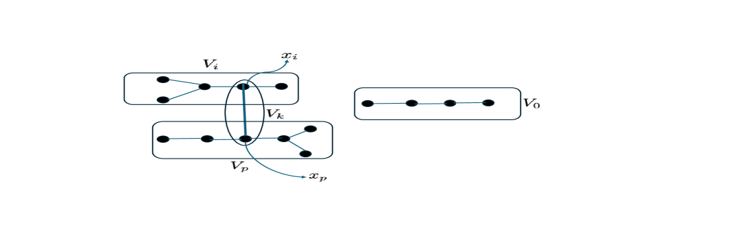
Figure 1: Figure 1: Figure explaining the structure of $G_{C}$

Claim: $V_{i}\cap V_{p}=\emptyset$.
If not, $X_{i}=X_{p}$ and there is a cycle in $G_{C}$ involving a path from $x_{p}$ to $x_{i}$ followed by the edge $\{x_{i},x_{p}\}$ due to $\{x_{i}=_{A}x_{p}\}\in E_{C}$. This is a contradiction due to our syntactic restriction and hence the claim holds.

In what follows, we let $var(\alpha)$ denote the set of variables that appear in the atomic formula $\alpha$ and extend this notation to a set of atomic formulas in the obvious way. We now partition $C$ as $C=\{C_{i},C_{p},C_{k},C_{0}\}$ where, as:

• $C_{i}=\{\alpha\,|\,\alpha\in C\,\text{and}\,var(\alpha)\subseteq V_{i}\}$.

• $C_{p}=\{\alpha\,|\,\alpha\in C\,\text{and}\,var(\alpha)\subseteq V_{p}\}$.

• $C_{k}=\{\alpha_{k}\}$.

• $C_{0}=\{\alpha\,|\,\alpha\in C\,\text{and}\,var(\alpha)\subseteq V_{0}\}$.

It is easy to verify that $\{C_{i},C_{p},C_{k},C_{0}\}$ is indeed a partition of $C$.

Lemma 4.

$\bigcap_{\ell\in[1,k]}L(\mathcal{B}(\alpha_{\ell}))\subseteq L(\mathcal{B}(C))$.

Proof 4.3.

It will suffice to show that $L(\mathcal{B}(C_{i}))\cap L(\mathcal{B}(C_{p}))\cap L(\mathcal{B}(C_{k}))\cap L(\mathcal{B}(C_{0}))\subseteq\mathcal{B}(C)$. We proceed by induction on $|E_{C}|$. Suppose $|E_{C}|=0$. In this case, our construction is essentially the one used for showing that Büchi automata are closed under intersection and the result follows easily.

So assume that $|E_{C}|>0$ and assume -without loss of generality- that $C=\{\alpha_{1},\alpha_{2},\dots,\alpha_{k-1},\alpha_{k}\}$ such that $\alpha_{k}=(x_{i}=_{A}x_{p})$ and hence $\{x_{i},x_{p}\}\in E_{C}$.

We now consider the partition $C=\{C_{i},C_{p},C_{k},C_{0}\}$ defined above.

Now consider the four hBAs $\mathcal{B}(C_{i})$, $\mathcal{B}(C_{p})$, $\mathcal{B}(C_{k})$ and $\mathcal{B}(C_{0})$. Then by the induction hypothesis:

• $L(\mathcal{B}(C_{i}))=\bigcap_{\alpha\in C_{i}}L(\mathcal{B}(\alpha))$.

• $L(\mathcal{B}(C_{p}))=\bigcap_{\alpha\in C_{p}}L(\mathcal{B}(\alpha))$.

• $L(\mathcal{B}(C_{k}))=L(\mathcal{B}(\alpha_{k}))$ (actually, this does not require the induction hypothesis).

• $L(\mathcal{B}(C_{0}))=\bigcap_{\alpha\in C_{0}}L(\mathcal{B}(\alpha))$.

Let $\boldsymbol{\sigma}\in\bigcap_{\ell\in[1,k]}L(\mathcal{B}(\alpha_{\ell}))$. This implies that $\boldsymbol{\sigma}\in L(\mathcal{B}(C_{i}))\cap L(\mathcal{B}(C_{p}))\cap L(\mathcal{B}(C_{k}))\cap L(\mathcal{B}(C_{0}))$. Assume that $\xi_{i}$ is an accepting run of $\mathcal{B}(C_{i})$ over $\boldsymbol{\sigma}$. Similarly, let $\xi_{p}$ be an accepting run of $\mathcal{B}(C_{p})$ over $\boldsymbol{\sigma}$, $\xi_{k}$ be an accepting run of $\mathcal{B}(\alpha_{k})$ over $\boldsymbol{\sigma}$ and $\xi_{0}$, an accepting run of $\mathcal{B}(C_{0})$ over $\boldsymbol{\sigma}$.

Let $\boldsymbol{\sigma}\in\bigcap_{\ell\in[1,k]}L(\mathcal{B}(\alpha_{\ell}))$. Assume that $\xi_{i}$ is an accepting run of $\mathcal{B}(C_{i})$ over $\boldsymbol{\sigma}$. Similarly, let $\xi_{p}$ be an accepting run of $\mathcal{B}(C_{p})$ over $\boldsymbol{\sigma}$, $\xi_{k}$ be an accepting run of $\mathcal{B}(\alpha_{k})$ over $\boldsymbol{\sigma}$ and $\xi_{0}$, an accepting run of $\mathcal{B}(C_{0})$ over $\boldsymbol{\sigma}$. We will asynchronously piece together these four runs into an accepting run $\xi$ of $\mathcal{B}(C)$ over $\boldsymbol{\sigma}$.

So assume that:

• $\xi_{i}=\mathbf{q}_{0,i}\mathbf{a}_{0,i}\mathbf{q}_{1,i}\mathbf{a}_{1,i}\mathbf{q}_{2,i}\dots$.

• $\xi_{p}=\mathbf{q}_{0,p}\mathbf{a}_{0,p}\mathbf{q}_{1,p}\mathbf{a}_{1,p}\mathbf{q}_{2,p}\dots$.

• $\xi_{k}=\mathbf{q}_{0,k}\mathbf{a}_{0,k}\mathbf{q}_{1,k}\mathbf{a}_{1,k}\mathbf{q}_{2,k}\dots$.

• $\xi_{0}=\mathbf{q}_{0,0}\mathbf{a}_{0,0}\mathbf{q}_{1,0}\mathbf{a}_{1,0}\mathbf{q}_{2,0}\dots$.

Now define $\xi^{\prime}_{i}=\mathbf{q}_{0,i}\mathbf{a}^{\prime}_{0,i}\mathbf{q}_{1,i}\mathbf{a}^{\prime}_{1,i}\mathbf{q}_{2,i}\dots$ where $\mathbf{a}^{\prime}_{t,i}(\ell)=\mathbf{a}_{t,i}(\ell)$ for each $x_{\ell}\in V_{i}$ and $\mathbf{a}^{\prime}_{t,i}(\ell)=\mathbf{a}_{t,0}(\ell)$ for each $x_{\ell}\in V_{0}$. Moreover, $\mathbf{q}_{t,i}(\alpha)=\mathbf{q}^{\prime}_{t,i}(\alpha)$ for every $\alpha\in i$ and $\mathbf{q}_{t,0}(\alpha)=\mathbf{q}^{\prime}_{t,0}(\alpha)$ for every $\alpha\in C_{0}$. It is easy to see that $\xi^{\prime}_{i}$ is also an accepting run of $\mathcal{B}(C_{i})$ over $\boldsymbol{\sigma}$. This is so since the states assumed by $\mathcal{B}(C_{i})$ when running over $\boldsymbol{\sigma}$ depend only on the components of $C$ that belong to $C_{i}$. The remaining components are “don’t care” conditions. For the same reason, $\xi^{\prime}_{i}$ is also an accepting run of $\mathcal{B}(C_{0})$ over $\boldsymbol{\sigma}$. In a similar manner, we can modify $\xi_{p}$ to $\xi^{\prime}_{p}$ and $\xi_{k}$ to $\xi^{\prime}_{k}$ such that:

• $\xi^{\prime}_{p}$ is an accepting run of $\mathcal{B}(C_{p})$ over $\boldsymbol{\sigma}$ and $\xi^{\prime}_{p}$ is an accepting run of $\mathcal{B}(C_{0})$ over $\boldsymbol{\sigma}$.

• $\xi^{\prime}_{k}$ is an accepting run of $\mathcal{B}(\alpha_{k})$ over $\boldsymbol{\sigma}$ and $\xi^{\prime}_{p}$ is an accepting run of $\mathcal{B}(C_{0})$ over $\boldsymbol{\sigma}$.

• $\mathbf{a}^{\prime}_{t,i}(\ell)=\mathbf{a}^{\prime}_{t,p}(\ell)=\mathbf{a}^{\prime}_{t,\alpha_{k}}(\ell)=\mathbf{a}^{\prime}_{t,C_{0}}(\ell)$ for every $t\geq 0$ and every $x_{\ell}\in V_{0}$.

• $\mathbf{q}^{\prime}_{t,i}(\alpha)=\mathbf{q}^{\prime}_{t,p}(\alpha)=\mathbf{q}^{\prime}_{t,\alpha_{k}}(alpha)=\mathbf{q}_{t,i}(\alpha)$ for every $t\geq 0$ and every $\alpha\in C_{i}$.

• $\mathbf{q}^{\prime}_{t,i}(\alpha)=\mathbf{q}^{\prime}_{t,p}(\alpha)=\mathbf{q}^{\prime}_{t,\alpha_{k}}(\alpha)=\mathbf{q}_{t,p}(\alpha)$ for every $t\geq 0$ and every $\alpha\in p$.

• $\mathbf{q}^{\prime}_{t,i}(\alpha_{k})=\mathbf{q}^{\prime}_{t,p}(\alpha_{k})=\mathbf{q}^{\prime}_{t,\alpha_{k}}(\alpha_{k})=\mathbf{q}_{t,k}(\alpha_{k})$ for every $t\geq 0$.

Now consider the run $\xi^{\prime}_{i}$ and $\xi^{\prime}_{k}$. Since $x_{i}\in V_{i}$ and $x_{i}=V_{k}$ it could be the case that for some $t$, $\mathbf{a}^{\prime}_{t,i}(i)\neq\mathbf{a}^{\prime}_{t,k}(i)$. Our task to remove such clashes while maintaining the conditions stated above to piece together the runs $\xi^{\prime}_{i}$, $\xi^{\prime}_{p}$ and $\xi^{\prime}_{k}$. This will produce an accepting run $\xi$ of $\mathcal{B}(C)$ over $\boldsymbol{\sigma}$.

We now construct $\xi=\mathbf{q}_{0,C}\mathbf{a}_{0,C}\mathbf{q}_{1,C}\mathbf{a}_{1,C}\mathbf{q}_{2,C}\dots$ incrementally. Recall that $\xi^{\prime}_{i}=\mathbf{q}_{0,i}\mathbf{a}^{\prime}_{0,i}\mathbf{q}_{1,i}\mathbf{a}^{\prime}_{1,i}\mathbf{q}_{2,i}\dots$, $\xi^{\prime}_{p}=\mathbf{q}_{0,p}\mathbf{a}^{\prime}_{0,p}\mathbf{q}_{1,p}\mathbf{a}^{\prime}_{1,p}\mathbf{q}_{2,p}\dots$ , $\xi^{\prime}_{k}=\mathbf{q}_{0,k}\mathbf{a}^{\prime}_{0,k}\mathbf{q}_{1,k}\mathbf{a}^{\prime}_{1,k}\mathbf{q}_{2,k}\dots$ and $\xi^{\prime}_{0}=\mathbf{q}_{0,0}\mathbf{a}^{\prime}_{0,0}\mathbf{q}_{1,0}\mathbf{a}^{\prime}_{1,0}\mathbf{q}_{2,0}\dots$ are accepting runs of $\mathcal{B}(C_{i})$, $\mathcal{B}(C_{p})$ , $\mathcal{B}(\alpha_{k}$ and $\mathcal{B}(C_{0})$ respectively over $\boldsymbol{\sigma}$ satisfying the properties stated above.

We start with $\mathbf{q}_{0,C}$ satisfying:

• $\mathbf{q}_{0,C}(\alpha)=\mathbf{q}_{0,i}(\alpha)$ for every $\alpha\in C_{i}$.

• $\mathbf{q}_{0,C}(\alpha)=\mathbf{q}_{0,p}(\alpha)$ for every $\alpha\in C_{p}$.

• $\mathbf{q}_{0,C}(\alpha_{k})=\mathbf{q}_{0,C_{k}}(\alpha_{k})$.

• $\mathbf{q}_{0,C}(\alpha)=\mathbf{q}_{0,0}(\alpha)$ for every $\alpha\in C_{0}$.

Now there are various cases to consider for fixing $\mathbf{a}_{0,C}$ based on which one can then fix $\mathbf{q}_{1,C}$.

• Suppose $\mathbf{a}_{0,i}(i),\mathbf{a}_{0,k}(i)\in\Sigma$ and $\mathbf{a}_{0,k}(p),\mathbf{a}_{0,p}(p)\in\Sigma$
  

  We note that since both $\mathcal{B}(C_{i})$ and $\mathcal{B}(C_{k})$ will run over the same trace $\boldsymbol{\sigma}(i)=\sigma_{i}$, we are assured that if $\mathbf{a}_{0,i}(i),\mathbf{a}_{0,k}(i)\in\Sigma$ then $\mathbf{a}_{0,i}(i)=\mathbf{a}_{0,k}(i)$. This is an invariant condition that will be maintained throughout the construction of $\xi$. A similar remark applies to the case $\mathbf{a}_{0,k}(p),\mathbf{a}_{0,p}(p)\in\Sigma$.

  Then we define $\mathbf{a}_{0,C}$ as:

  • $\mathbf{a}_{0,C}(\ell)=\mathbf{a}_{0,i}(\ell)$ if $x_{l}\in V_{i}$.

  • $\mathbf{a}_{0,C}(\ell)=\mathbf{a}_{0,p}(\ell)$ if $x_{l}\in V_{p}$.

  • $\mathbf{a}_{0,C}(\ell)=\mathbf{a}_{0,k}(\ell)$ if $x_{l}\in V_{k}$.

  • $\mathbf{a}_{0,C}(\ell)=\mathbf{a}_{0,C_{0}}(\ell)$ if $x_{l}\in V_{0}$.

  This leads to $\mathbf{q}_{1,C}$ given by:

  • $\mathbf{q}_{1,C}(\alpha)=\mathbf{q}_{1,i}(\alpha)$ if $\alpha\in C_{i}$.

  • $\mathbf{q}_{1,C}(\alpha)=\mathbf{q}_{1,p}(\alpha)$ if $\alpha\in C_{p}$.

  • $\mathbf{q}_{1,C}(\alpha)=\mathbf{q}_{1,k}(\alpha)$ if $\alpha\in C_{k}$ (in other words, $\alpha=\alpha_{k}$).

  • $\mathbf{q}_{1,C}(\alpha)=\mathbf{q}_{1,0}(\alpha)$ if $\alpha\in C_{0}$.

  Thus we advance all the four components according to the runs $\xi^{\prime}_{i}$, $\xi^{\prime}_{p}$, $\xi^{\prime}_{k}$ and $\xi^{\prime}_{0}$. We note that

• Suppose $\mathbf{a}_{0,i}(i)\in Sigma$, $\mathbf{a}_{0,k}(i)=\epsilon$ and $\mathbf{a}_{0,k}(p),\mathbf{a}_{0,p}(p)\in\Sigma$
  

  Then we define $\mathbf{a}_{0,C}$ as:

  • $\mathbf{a}_{0,C}(\ell)=\epsilon$ if $x_{l}\in V_{i}$.

  • $\mathbf{a}_{0,C}(\ell)=\mathbf{a}_{0,p}(\ell)$ if $x_{l}\in V_{p}$.

  • $\mathbf{a}_{0,C}(\ell)=\mathbf{a}_{0,k}(\ell)$ if $x_{l}\in V_{k}$.

  • $\mathbf{a}_{0,C}(\ell)=\mathbf{a}_{0,C_{0}}(\ell)$ if $x_{l}\in V_{0}$.

  This leads to $\mathbf{q}_{1,C}$ given by:

  • $\mathbf{q}_{1,C}(\alpha)=\mathbf{q}_{0,i}(\alpha)$ if $\alpha\in C_{i}$.

  • $\mathbf{q}_{1,C}(\alpha)=\mathbf{q}_{1,p}(\alpha)$ if $\alpha=C_{p}$.

  • $\mathbf{q}_{1,C}(\alpha)=\mathbf{q}_{1,k}(\alpha)$ if $\alpha\in C_{k}$ (in other words, $\alpha=\alpha_{k}$).

  • $\mathbf{q}_{1,C}(\alpha)=\mathbf{q}_{1,C_{0}}(\alpha)$ if $\alpha\in C_{0}$.

  Thus we “freeze” the component $V_{i}$ and let the components $V_{p}$, $V_{k}$ and $V_{0}$ advance according to the runs $\xi^{\prime}_{p}$, $\xi^{\prime}_{k}$ and $\xi^{\prime}_{0}$.

• Suppose $\mathbf{a}_{0,i}(i)=\epsilon$, $\mathbf{a}_{0,k}(i)\in\Sigma$ and $\mathbf{a}_{0,k}(p),\mathbf{a}_{0,p}(p)\in\Sigma$
  

  Then we define $\mathbf{a}_{0,C}$ as:

  • $\mathbf{a}_{0,C}(\ell)=\mathbf{a}_{0,i}(\ell)$ if $x_{l}\in V_{i}$.

  • $\mathbf{a}_{0,C}(\ell)=\epsilon$ if $x_{l}\in V_{p}$.

  • $\mathbf{a}_{0,C}(\ell)=\epsilon$ if $x_{l}\in V_{k}$.

  • $\mathbf{a}_{0,C}(\ell)=\mathbf{a}_{0,C_{0}}(\ell)$ if $x_{l}\in V_{0}$.

  This leads to $\mathbf{q}_{1,C}$ given by:

  • $\mathbf{q}_{1,C}(\alpha)=\mathbf{q}_{1,i}(\alpha)$ if $\alpha\in i$.

  • $\mathbf{q}_{1,C}(\alpha)=\mathbf{q}_{0,p}(\alpha)$ if $\alpha=C_{p}$.

  • $\mathbf{q}_{1,C}(\alpha)=\mathbf{q}_{0,k}(\alpha)$ if $\alpha\in C_{k}$ (in other words, $\alpha=\alpha_{k}$).

  • $\mathbf{q}_{1,C}(\alpha)=\mathbf{q}_{1,C_{0}}(\alpha)$ if $\alpha\in C_{0}$.

  Thus in this case, we “freeze” the components $V_{p}$ and $V_{k}$ and let the components $V_{i}$ and $V_{0}$ advance according to the runs $\xi^{\prime}_{i}$ and $\xi^{\prime}_{0}$.

• Suppose $\mathbf{a}_{0,i}(i)=\epsilon$, $\mathbf{a}_{0,k}(i)=\epsilon$ and $\mathbf{a}_{0,k}(p),\mathbf{a}_{0,p}(p)\in\Sigma$.
  

  Then we define $\mathbf{a}_{0,C}$ as:

  • $\mathbf{a}_{0,C}(\ell)=\mathbf{a}_{0,i}(\ell)$ if $x_{l}\in V_{i}$.

  • $\mathbf{a}_{0,C}(\ell)=\mathbf{a}_{0,p}(\ell)$ if $x_{l}\in V_{p}$.

  • $\mathbf{a}_{0,C}(\ell)=\mathbf{a}_{0,k}(\ell)$ if $x_{l}\in V_{k}$.

  • $\mathbf{a}_{0,C}(\ell)=\mathbf{a}_{0,C_{0}}(\ell)$ if $x_{l}\in V_{0}$.

  This leads to $\mathbf{q}_{1,C}$ given by:

  • $\mathbf{q}_{1,C}(\alpha)=\mathbf{q}_{1,i}(\alpha)$ if $\alpha\in C_{i}$.

  • $\mathbf{q}_{1,C}(\alpha)=\mathbf{q}_{1,p}(\alpha)$ if $\alpha\in C_{p}$.

  • $\mathbf{q}_{1,C}(\alpha)=\mathbf{q}_{1,k}(\alpha)$ if $\alpha\in k$ (in other words, $\alpha=\alpha_{k}$).

  • $\mathbf{q}_{1,C}(\alpha)=\mathbf{q}_{1,C_{0}}(\alpha)$ if $\alpha\in C_{0}$.

  Thus we advance all the four components according to the associated runs.

• Suppose $\mathbf{a}_{0,p}(p)\in Sigma$, $\mathbf{a}_{0,k}(p)=\epsilon$ and $\mathbf{a}_{0,i}(i),\mathbf{a}_{0,k}(i)\in\Sigma$
  Then we define $\mathbf{a}_{0,C}$ as:

  • $\mathbf{a}_{0,C}(\ell)=\epsilon$ if $x_{l}\in V_{p}$.

  • $\mathbf{a}_{0,C}(\ell)=\mathbf{a}_{0,i}(\ell)$ if $x_{l}\in V_{i}$.

  • $\mathbf{a}_{0,C}(\ell)=\mathbf{a}_{0,k}(\ell)$ if $x_{l}\in V_{k}$.

  • $\mathbf{a}_{0,C}(\ell)=\mathbf{a}_{0,C_{0}}(\ell)$ if $x_{l}\in V_{0}$.

  This leads to $\mathbf{q}_{1,C}$ given by:

  • $\mathbf{q}_{1,C}(\alpha)=\mathbf{q}_{1,i}(\alpha)$ if $\alpha\in C_{i}$.

  • $\mathbf{q}_{1,C}(\alpha)=\mathbf{q}_{0,p}(\alpha)$ if $\alpha=C_{p}$.

  • $\mathbf{q}_{1,C}(\alpha)=\mathbf{q}_{1,k}(\alpha)$ if $\alpha\in C_{k}$ (in other words, $\alpha=\alpha_{k}$).

  • $\mathbf{q}_{1,C}(\alpha)=\mathbf{q}_{1,C_{0}}(\alpha)$ if $\alpha\in C_{0}$.

  Thus we freeze the component $V_{p}$ and let the components $V_{i}$, $V_{k}$ and $V_{0}$ advance according to the runs $\xi^{\prime}_{i}$, $\xi^{\prime}_{k}$ and $\xi^{\prime}_{0}$ respectively.

• Suppose $\mathbf{a}_{0,p}(p)=\epsilon$, $\mathbf{a}_{0,k}(p)\in Sigma$ and $\mathbf{a}_{0,i}(i),\mathbf{a}_{0,k}(i)\in\Sigma$
  

  Then we define $\mathbf{a}_{0,C}$ as:

  • $\mathbf{a}_{0,C}(\ell)=\mathbf{a}_{0,p}(\ell)$ if $x_{l}\in V_{p}$.

  • $\mathbf{a}_{0,C}(\ell)=\epsilon$ if $x_{l}\in V_{k}$.

  • $\mathbf{a}_{0,C}(\ell)=\epsilon$ if $x_{l}\in V_{i}$.

  • $\mathbf{a}_{0,C}(\ell)=\mathbf{a}_{0,C_{0}}(\ell)$ if $x_{l}\in V_{0}$.

  This leads to $\mathbf{q}_{1,C}$ given by:

  • $\mathbf{q}_{1,C}(\alpha)=\mathbf{q}_{1,p}(\alpha)$ if $\alpha\in C_{p}$.

  • $\mathbf{q}_{1,C}(\alpha)=\mathbf{q}_{0,k}(\alpha)$ if $\alpha=C_{k}$.

  • $\mathbf{q}_{1,C}(\alpha)=\mathbf{q}_{0,i}(\alpha)$ if $\alpha\in C_{i}$ (in other words, $\alpha=\alpha_{k}$).

  • $\mathbf{q}_{1,C}(\alpha)=\mathbf{q}_{1,C_{0}}(\alpha)$ if $\alpha\in C_{0}$.

  Thus we freeze the components $V_{k}$ and $V_{i}$ and let the components $V_{p}$ and $V_{0}$ advance according to the associated runs.

  The case $\mathbf{a}_{0,k}(i)=\mathbf{a}_{0,k}(p)=\epsilon$ can be ruled out by the definition of $\mathcal{B}(\alpha_{k})$. Hence the cases considered above all that are needed.

Now assume inductively that we have constructed the finite run $(\boldsymbol{\tau}_{i},\boldsymbol{\tau}_{k},\boldsymbol{\tau}_{p},\boldsymbol{\tau}_{0})$ of $\mathcal{B}(C)$ over $\boldsymbol{\sigma}$ leading to $(\mathbf{q}_{i},\mathbf{q}_{k},\mathbf{q}_{p},\mathbf{q}(0))$ where:

• $\mathbf{q}_{i}(\alpha)=\mathbf{q}_{|\boldsymbol{\tau}_{i}|,i}(\alpha)$ for every $\alpha\in C_{i}$.

• $\mathbf{q}_{k}(\alpha)=\mathbf{q}_{|\boldsymbol{\tau}_{k}|,i}(\alpha)$ for every $\alpha\in C_{k}$.

• $\mathbf{q}_{p}(\alpha)=\mathbf{q}_{|\boldsymbol{\tau}_{p}|,i}(\alpha)$ for every $\alpha\in C_{p}$.

• $\mathbf{q}_{0}(\alpha)=\mathbf{q}_{|\boldsymbol{\tau}_{0}|,i}(\alpha)$ for every $\alpha\in C_{0}$.

We note that $|\boldsymbol{\tau}_{i}|$ is the number of non-$\epsilon$ moves that have been made by the component $V_{i}$ along the finite run $(\boldsymbol{\tau}_{i},\boldsymbol{\tau}_{k},\boldsymbol{\tau}_{p},\boldsymbol{\tau}_{0})$. Then again by considering the various cases specified in the basis step but now applied at $(\mathbf{q}_{i},\mathbf{q}_{p},\mathbf{q}_{k},\mathbf{q}_{0})$ we extend the run $(\boldsymbol{\tau}_{i},\boldsymbol{\tau}_{k},\boldsymbol{\tau}_{p},\boldsymbol{\tau}_{0})$ to $(\boldsymbol{\tau}^{\prime}_{i},\boldsymbol{\tau}^{\prime}_{k},\boldsymbol{\tau}^{\prime}_{p},\boldsymbol{\tau}^{\prime}_{0})$

Using the fact that $\xi^{\prime}_{i}$, $\xi^{\prime}_{k}$, $\xi^{\prime}_{p}$ and $\xi^{\prime}_{0}$ are accepting runs of $\mathcal{B}(C_{i})$, $\mathcal{B}(C_{k})$, $\mathcal{B}(C_{p})$ and $\mathcal{B}(C_{0})$ respectively over $\boldsymbol{\sigma}$ we can now show that in the limit we will obtain $\xi$, an accepting run $\mathcal{B}(C)$ over $\boldsymbol{\sigma}$.

The disjunction of the clauses   $\{C_{j}\}$.

We now have the hBAs $\mathcal{B}(C_{j})$ for each $j\in[1,m]$. Now using the fact that hBAs are closed under union we can easily construct the hBA $\mathcal{B}(\mathbf{C})$ that satisfies $L(\mathcal{B}(\mathbf{C}))=\parallel\mathbf{C}\parallel$.

4.4 The main result

Finally we show that it is decidable whether the lanaguage recognized by a hBA is non-empty. To do so we first note that the hBA $\mathcal{B}=(Q,\delta,Q_{in},F)$ induces the directed graph $G_{\mathcal{B}}=(Q,E,\lambda_{\mathcal{B}})$ where $e=(q,q^{\prime})\in E$ iff there exists $\mathbf{a}$ such that $\lambda_{\mathcal{B}}(e)=\mathbf{a}$ and $q^{\prime}\in\delta(q,\mathbf{a})$.

Lemma 5.

Let $\mathcal{B}$ be an hBA and $G_{\mathcal{B}}=(Q,E,\lambda_{\mathcal{B}})$, its induced directed graph. Then whether $L(\mathcal{B})\neq\emptyset$ can determined in time $O(|Q|+|E|)$.

The proof is very similar to the one for Büchi automata. The main difference is the $G_{\mathcal{B}}=(Q,E,\lambda_{\mathcal{B}})$ must have a reachable non-trivial strongly component $X$ that contains an accepting state of $\mathcal{B}$ and for each $i\in[1,n]$ there exists $(q,q^{\prime})\in E$ such that $\lambda_{\mathcal{B}}((q,q^{\prime}))(i)\in\Sigma$ and $q,q^{\prime}\in X$.

The main result of this section now follows.

Theorem 6.

The satisfibalility problem for LPrL can be decided in time $2^{|\psi|}$.

In the next section, we will write $\mathcal{B}(\psi)$ instead of $\mathcal{B}(\mathbf{C})$ to emphasize its association with $\psi$.

5 The Model Checking Problem

We recall that we are given a family of Kripke structures $\{K_{i}\}_{i}$ and the specification $\psi$ in normal form as defined in section 4. We assume $K_{i}=(S_{i},s_{in,i},R_{i},AP_{i},\lambda_{i})$ and $M_{i}$ is the set of traces of $K_{i}$ for each $i$. For convenience, we set $\mathbf{M}=(M_{1},M_{2},\dots,M_{n})$ and $\mathbf{K}=\{K_{i}\}_{i}$.

As a first step, we will characterize when $\mathbf{M}$ is a model of $\psi$ using objects named $(\mathbf{M},\psi)$ trees. In essence, a $(\mathbf{M})$ tree is the game tree arising in the game theoretic semantics of first order logic and a $(\mathbf{M},\psi)$ tree is a winning strategy for the “prover”. However, we will not need this machinery here and hence we will not introduce it here.

We will then design a Büchi word automaton $\mathcal{B}(\mathbf{K},\psi)$ and show that this automaton has an accepting run iff there exists a $\mathcal{B}(\mathbf{K},\psi)$ tree. Finally, we will establish that the emptiness problem for $\mathcal{B}(\mathbf{K},\psi)$ is decidable.

5.1 $(\mathbf{M},\psi)$ trees

To illustrate the notion of a $(\mathbf{M},\psi)$ tree, consider the system consisting of three Kripke structures and the specification $\forall x_{1}\exists x_{2}\forall x_{3}(\varphi^{1}(x_{1})\equiv\varphi^{2}(x_{2})\wedge x_{2}=x_{3})$ as shown in Figure 1(a). To minimize clutter, we have not spelled out $AP$ and the action labels such $a_{1}$, $b_{2}$, $c_{3}$ etc. We have also not spelled out the LTL formulas $\varphi^{1}$ and $\varphi^{2}$ used in the matrix of $\psi$.

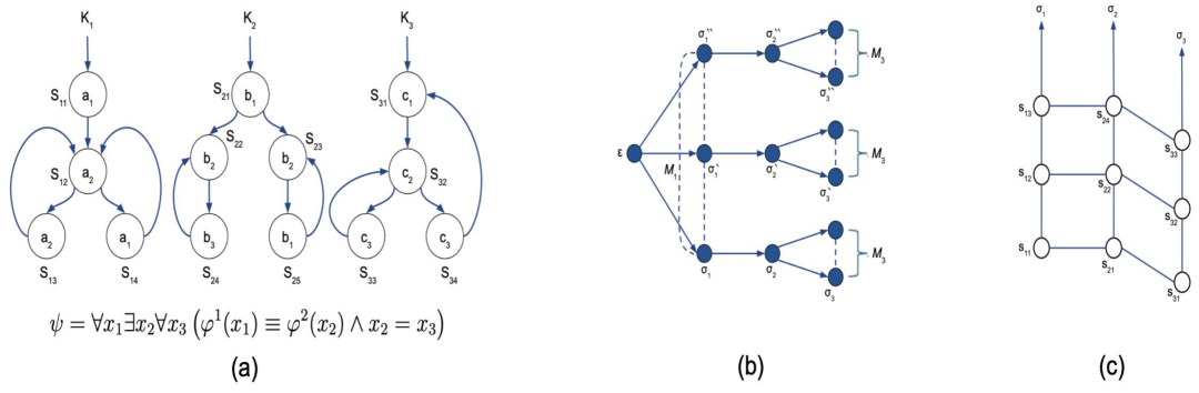
Figure 2: Figure 1: Figure explaining the various steps in Model Checking a given LPrL formula.

A key observation is that the intended relationships between the traces of the three Kripke structures -as specified by the prefix of $\psi$- can be represented as a tree. The root of the tree will be labeled with $\epsilon$ and the nodes at depth $i$ will be labeled with traces in $M_{i}$. In Figure 1(a), since $x_{1}\in\mathsf{VAR}^{\forall}$, for each trace $\sigma_{1}$ in $M_{1}$ there will be a unique node at depth $1$ labeled with $\sigma_{1}$. Further, since $x_{2}\in\mathsf{VAR}^{\exists}$, each node at depth $1$ will have a unique successor node labeled with a trace in $M_{2}$. Similarly, each node at depth $2$ will have, corresponding to each trace $\sigma_{3}$ in $M_{3}$, a successor node labeled with $\sigma_{3}$. It is important to note that edges in the tree merely capture the structure of the prefix of the specification. They do not imply any kind of a causal relationship between the traces associated with the corresponding nodes. In Figure 1(b) we have illustrated the structure of an $\mathbf{M}$ tree for the model shown in Figure 1(a). Finally, in Figure 1(c) we highlight the fact each node of the tree is labeled by a trace.

Now consider a branch, in terms of the labels of the nodes on the branch, say, $\epsilon\,\sigma_{1}\,\sigma_{2}\,\sigma_{3}$ of this $\mathbf{M}$ tree. If $\mathbf{M}$ is to be model of $\psi$, then it must be the case that $v([\mathbf{C}])^{(x_{1},x_{2},x_{3})}_{(\sigma_{1},\sigma_{2},\sigma_{3})})=True$ for any valuation $v$ over $\mathbf{M}$ where $\mathbf{C}$ is the matrix of the specification. In this sense, a $(\mathbf{M},\psi)$ tree is a $\mathbf{M}$ tree in which every branch satisfies the matrix of the specification.

To formalize these ideas, we begin with some tree preliminaries. Let $D$ be a non-empty set of directions. Then a $D$-tree is a prefix-closed subset $T\subseteq D^{*}$. Thus if $\eta d\in T$ and $d\in D$ then $\eta\in T$. The members of $T$ are the nodes and $\epsilon$ is the root of $T$. Let $\eta,\eta^{\prime}\in T$. Then $\eta^{\prime}$ is a successor of $\eta$ iff there exists $d\in D$ such that $\eta^{\prime}=\eta d$. We let $succ(\eta)$ be the set of successors of the node $\eta$. A leaf node is a node whose set of successors is empty. The depth of the node $\eta$ is the length of the sequence $\eta$. The tree $T$ is of finite depth if there exists a non-negative integer $k_{T}$ such that $\mid\eta\mid\leq k_{T}$ for every (leaf) node $\eta$ in $T$. We will only be dealing trees of depth $n$ here.

A (finite) path is a sequence of nodes $\pi=\eta_{0}\eta_{1}\dots\eta_{k}$ such that $\eta_{0}=\epsilon$ and $\eta_{l+1}\in succ(\eta_{l})$ for $0\leq l<k$. A branch is a maximal path. In other words, it is a finite path whose last node is a leaf node.

Given a set of labels $Y$, an $Y$-labeled $D$-tree is a pair $(T,\mathcal{T})$ where $T$ is a $D$-tree and $\mathcal{T}:T\to Y$. The labeling function $\mathcal{T}$ is extended to paths in the obvious way with the convention $\mathcal{T}(\epsilon)=\epsilon$.

We set $M=\bigcup_{i}M_{i}$ and let $\mathbb{R}_{\geq 0}$ be the set of non-negative reals. Then an $(\mathbf{M})$ tree is a $M\text{-labeled}$ $\mathbb{R}_{\geq 0}\text{-tree}$ $(T,\mathcal{T})$ which satisfies the following conditions for each node $\eta$:

• $depth(\eta)\leq n$.

• If $0<depth(\eta)=i\leq n$ then $\mathcal{T}(\eta)\in M_{i}$.

• If $0<depth(\eta)=i<n$ and $x_{i+1}=\mathsf{VAR}^{\exists}$ then there exists $\sigma\in M_{i+1}$ and a node $\eta^{\prime}$ such that $\mathcal{T}(\eta^{\prime})=\sigma$ and $succ(\eta)=\{\eta^{\prime}\}$.

• If $0<depth(\eta)=i<n$ and $x_{i+1}=\mathsf{VAR}^{\forall}$ then for every $\sigma\in M_{i+1}$ there exists a unique node $\eta^{\prime}\in succ(\eta)$ such that $\mathcal{T}(\eta^{\prime})=\sigma$.

We note that the branching degree of an $(\mathbf{M})$ tree will be at most $max\{\mid M_{i}\mid\}$ which, being a subset of $\Sigma^{\omega}$, will have at most the cardinality of the set of non-negative reals.

We now define a $(\mathbf{M},\psi)$ tree to be a $(\mathbf{M})$ tree which satisfies: If $br=\eta_{0}\eta_{1}\dots\eta_{n}$ is a branch of $T$ with $\mathcal{T}(br)=\boldsymbol{\sigma}=(\sigma_{1},\sigma_{2},\dots,\sigma_{n})$ then $v([\mathbf{C}]^{\mathbf{x}}_{\boldsymbol{\sigma}})=True$ where $v$ is a valuation over $\mathbf{M}$ and $\mathbf{C}$ is the matrix of $\psi$. This leads to:

Proposition 5.1.

$\mathbf{M}\models\psi$ iff there exists a $(\mathbf{M},\psi)$ tree.

Proof 5.2.

Follows easily from the semantic definitions. Here again, it is worth noting that a $(\mathbf{M},\psi)$ tree represents a winning strategy for the “prover” to show that $\psi$ is satisfied by the model $\mathbf{M}$ in the game theoretic semantics of first order logic.

5.2 An automata theoretic solution

We will first design a word automaton $\mathcal{B}(\mathbf{K})$ which will admit a run iff there exists a $(\mathbf{M})$ tree. Using $\mathcal{B}(\psi)$ constructed in the previous section, we will then convert $\mathcal{B}(\mathbf{K})$ to the automaton $\mathcal{B}(\mathbf{K},\psi)$ such that this automaton admits an accepting run iff there exists a $(\mathbf{M},\psi)$ tree. Finally we will show that is decidable whether a $\mathcal{B}(\mathbf{K},\psi)$ tree admits an accepting run.

We start with some preliminaries. Let $\{K_{i}\}_{i}$ with $K_{i}=(S_{i},s_{in,i},R_{i},AP_{i},\lambda_{i})$ and $M_{i}$, the set of traces of $K_{i}$ for each $i$. As before, $\mathbf{M}=(M_{1},M_{2},\dots,M_{n})$ and $\mathbf{K}=\{K_{i}\}_{i}$. For each $i$, we next define the transition relation $\longrightarrow_{i}\subseteq S_{i}\times\Sigma\times S_{i}$ given by:

$s\stackrel{{\scriptstyle a}}{{\longrightarrow_{i}}}s^{\prime}$ iff $(s,s^{\prime})\in R_{i}$ and $\lambda_{i}(s)=a$.

We now define $\mathbf{S}=S_{1}\times S_{2}\dots\times S_{n}$ and the transition relation $\longrightarrow\subseteq\mathbf{S}\times\Sigma^{n}\times\mathbf{S}$ as:

$\mathbf{s}\stackrel{{\scriptstyle\mathbf{a}}}{{\longrightarrow}}\mathbf{s}^{\prime}$ iff $\mathbf{s}(i)\stackrel{{\scriptstyle\mathbf{a}(i)}}{{\longrightarrow_{i}}}\mathbf{s}^{\prime}(i)$ for each $i$.

We term members of $\mathbf{S}$ to be micro states and define a macro state to be a non-empty set of micro states. For brevity, we will from now just say state instead of macro state. Let $\mathbf{U}$ be the set of states.

We now define the transition relation $\Longrightarrow$ as follows. Suppose $\mathbf{u},\mathbf{u}^{\prime}\in\mathbf{U}$ and $next\subseteq\mathbf{u}\times\Sigma^{n}\times\mathbf{u}^{\prime}$. Then $\mathbf{u}\stackrel{{\scriptstyle next}}{{\Longrightarrow}}\mathbf{u}^{\prime}$ iff the following conditions are satisfied.

• If $(\mathbf{s},\mathbf{a},\mathbf{s}^{\prime})\in next$ then $\mathbf{s}\stackrel{{\scriptstyle\mathbf{a}}}{{\longrightarrow}}\mathbf{s}^{\prime}$. Thus $next$ will relate the micro states in $\mathbf{u}$ to the micro states in $\mathbf{u}^{\prime}$ via an $n$-tuples of actions.

• If $\mathbf{s}\in\mathbf{u}$ then there exists $\mathbf{a}\in\Sigma^{n}$ and $\mathbf{s}^{\prime}\in\mathbf{u}^{\prime}$ such that $(\mathbf{s},\mathbf{a},\mathbf{s}^{\prime})\in next$. Thus no micro state in $\mathbf{u}$ will get stuck.

• If $\mathbf{s}^{\prime}\in\mathbf{u}^{\prime}$ then there exists $\mathbf{a}\in\Sigma^{n}$ and $\mathbf{s}\in\mathbf{u}$ such that $(\mathbf{s},\mathbf{a},\mathbf{s}^{\prime})\in next$. Thus there are no spurious micro states in $\mathbf{u}^{\prime}$.

• Suppose $x_{i}\in VAR{\forall}$ and $(\mathbf{s},\mathbf{a},\mathbf{s}^{\prime})\in next$. Then for every $(\mathbf{s}(i),s^{\prime\prime})\in R_{i}$ there exists $(\mathbf{s}_{1},\mathbf{b},\mathbf{s}_{2})\in next$ such that the following conditions are satisfied:

  • For $\ell\in[1,i]$, $\mathbf{s}(\ell)=\mathbf{s}_{1}(\ell)$.

  • For $1\leq\ell<i$, $\mathbf{s}^{\prime}(\ell)=\mathbf{s}_{2}(\ell)$.

  • $\mathbf{s}_{2}(i)=s^{\prime\prime}$.

  Thus this requirement states that the components appearing earlier than $x_{i}$ in the prefix can move as before while the component $K_{i}$ can freely pick any successor of $\mathbf{s}(i)$.

• Suppose $(\mathbf{s}_{1},\mathbf{a},\mathbf{s}_{2}),(\mathbf{s}^{\prime}_{1},\mathbf{b},\mathbf{s}^{\prime}_{2})\in next$ and $x_{\ell}\in VAR^{\exists}$ for every $\ell\in[1,i]$. Then $\mathbf{s}_{1}(\ell)=\mathbf{s}^{\prime}_{1}(\ell)$ and $\mathbf{s}_{2}(\ell)=\mathbf{s}^{\prime}_{2}(\ell)$ for every $\ell\in[1,i]$.

  This requirement says that if there is an initial prexix of existentially quantified variables then the the corresponding components will always pick the same unique successor state.

We now define the automaton $\mathcal{B}(\mathbf{K})$ to be the structure $\mathcal{B}(\mathbf{K})=(\mathbf{U},\mathbf{u}_{in},\Longrightarrow)$ where $\mathbf{U}$ and $\Longrightarrow$ are as defined above and:
$\mathbf{u}_{in}=\{\mathbf{s}_{in}\}$ where $\mathbf{s}_{in}(i)=s_{in,i}$ for every $i$.

A run of $\mathcal{B}(\mathbf{K})$ is an infinite sequence $\xi=\mathbf{u}_{0}\,next_{0}\,\mathbf{u}_{1}\,next_{1}\,\mathbf{u}_{2}\dots$ such that:

• $\mathbf{u}_{0}=\mathbf{u}_{in}$.

• $\mathbf{u}_{k}\stackrel{{\scriptstyle next_{k}}}{{\Longrightarrow}}\mathbf{u}_{k+1}$ for every $k\geq 0$.

Our aim is to show that $\mathcal{B}(\mathbf{K})$ admits a run iff there exists a $(\mathbf{M})$ tree.

5.3 A run of $\mathcal{B}(\mathbf{K})$ induces a $(\mathbf{K})$ tree

Let $\mathcal{B}(\mathbf{K})=(\mathbf{U},\mathbf{u}_{in},\Longrightarrow)$ be as defined above.

Suppose $\xi=\mathbf{u}_{0}\,next_{0}\,\mathbf{u}_{1}\,next_{1}\,\mathbf{u}_{2}\dots$ is a run of $\mathcal{B}(\mathbf{K})$. We will inductively construct the sequence of labeled trees $(T_{i},\mathcal{T}_{i})$ such that $(T_{n},\mathcal{T}_{n})$ is a $(\mathbf{M})$ tree. To do so, we first introduce some convenient notations.

A micro run is an infinite sequence $\mathbf{s}_{0}\,\mathbf{a}_{0}\,\mathbf{s}_{1}\,\mathbf{a}_{1}\,\mathbf{s}_{2}\dots$ such that:

• $\mathbf{s}_{0}=\mathbf{s}_{in}$ where $\mathbf{s}_{in}(i)=s_{in,i}$ for every $i$.

• $\mathbf{s}_{\ell}\stackrel{{\scriptstyle\mathbf{a}_{\ell}}}{{\longrightarrow}}\mathbf{s}_{\ell+1}$ for all $\ell\geq 0$.

Let $\rho=\mathbf{s}_{0}\,\mathbf{a}_{0}\,\mathbf{s}_{1}\mathbf{a}_{1}\mathbf{s}_{2}\dots$ be a micro run. Then $st(\rho)=\mathbf{s}_{0}\,\mathbf{s}_{1}\dots$. Further, $act(\rho)=\mathbf{a}_{0}\,\mathbf{a}_{1}\dots$. We next define $act(\rho)(i)=\mathbf{a}_{0}(i)\,\mathbf{a}_{1}(i)\dots$ for $i\in[1,n]$. We note that $act(\rho)(i)\in\Sigma^{\omega}$ for each $i$. This leads to:

$ACT(\rho)=(act(\rho)(1),act(\rho)(2),\dots,act(\rho)(n))$. We note that $CT(\rho)\in(\Sigma^{\omega})^{n}$.

We will say that the micro run $\rho=\mathbf{s}_{0}\,\mathbf{a}_{0}\,\mathbf{s}_{1}\,\mathbf{a}_{1}\,\mathbf{s}_{2}\dots$ is induced by the run $\xi=\mathbf{u}_{0}\,next_{0}\,\mathbf{u}_{1}\,next_{1}\,\mathbf{u}_{2}\dots$ (of $\mathcal{B}(\mathbf{K})$) iff $(\mathbf{s}_{\ell},\mathbf{a}_{l},\mathbf{s}_{\ell+1})\in next_{l}$ for every $\ell\geq 0$. Through the rest of this sub-section, we fix a run $\xi$ and let $\mathbf{P}_{\xi}$ denote the set of micro runs induced by $\xi$. Since $\xi$ is fixed, we will often write $\mathbf{P}$ instead of $\mathbf{P}_{\xi}$.

Next for $\mathbf{s}\in\mathbf{S}$ and each $i$, we define $\mathbf{s}[i]=(\mathbf{s}(1),\mathbf{s}(2),\dots,\mathbf{s}(i))$. Similarly, for $\mathbf{a}\in\Sigma^{n}$ and each $i$, we define $\mathbf{a}[i]=(\mathbf{a}(1),\mathbf{a}(2),\dots,\mathbf{a}(i))$. For the micro run $\rho$, this leads to, $\rho[i]=\mathbf{s}_{0}[i]\,\mathbf{a}_{0}[i]\,\mathbf{s}_{1}[i]\,\mathbf{a}_{1}[i]\,\mathbf{s}_{2}[i]\dots$ where $\rho=\mathbf{s}_{0}\,\mathbf{a}_{0}\,\mathbf{s}_{1}\,\mathbf{a}_{1}\,\mathbf{s}_{2}\dots$. Finally, $ACT(\rho)[i]=(\sigma_{1},\sigma_{2},\dots,\sigma_{i})$ where $ACT(\rho)=(\sigma_{1},\sigma_{2},\dots,\sigma_{n})$. We can define $(T,\mathcal{T})$.

We begin with $T_{0}=\{\epsilon\}$ and $\mathcal{T}_{0}(\epsilon)=\epsilon$.

First suppose $x_{1}\in\mathsf{VAR}^{\exists}$. Then we arbitrarily pick $\rho\in\mathbf{P}$ and set $V_{1}=\{\rho[1]\}$. We then define $\mathcal{T}_{1}(\rho[1])=ACT(\rho)(1)$. Furthermore, $succ(\epsilon)=V_{1}$. We will show below that neither the identity of the node in $V_{1}$ nor its label will depend on the choice of $\rho$.

Next suppose $x_{1}\in\mathsf{VAR}^{\forall}$. Then we define $V_{1}=\{\rho[1]\,|\,\rho\in\mathbf{P}\}$. For each $\rho[1]\in V_{1}$ we define $\mathcal{T}_{1}(\rho[1])=ACT(\rho)(1)$. Furthermore, $succ(\epsilon)=V_{1}$.

Assume inductively, that for some $i$ with $1\leq i<n$, the tree $(T_{i},\mathcal{T}_{i})$ of depth $i$ has been constructed. Assume further that if $\eta_{0}\eta_{1}\dots\eta_{i}$ is a branch of $(T_{i},\mathcal{T}_{i})$, then there exists $\rho\in\mathbf{P}$ such $\eta_{0}=\epsilon$ and $\eta_{\ell+1}=\eta_{\ell}\rho[\ell+1]$ for $0\leq\ell<i$. This hypothesis clearly holds for $i=1$. To extend $(T_{i},\mathcal{T}_{i})$ to $(T_{i+1},\mathcal{T}_{i+1})$ we again consider two cases.

Suppose $x_{i+1}\in VAR^{\exists}$. Then for each leaf node $\eta$ in $(T_{i},\mathcal{T}_{i})$ with $last(\eta)=\rho[i]$, we arbitrarily pick $\rho^{\prime}\in\mathbf{P}$ such that $\rho^{\prime}[i]=\rho[i]$ and add $\rho[i+1]$ to $V_{i+1}$. In addition, we define $succ(\eta)=\{\eta\rho^{\prime}[i+1]\}$ and set $\mathcal{T}_{i+1}(\eta\rho^{\prime}[i+1])=ACT(\rho^{\prime})(i+1)$. Here $last(\eta)$ is the last member in the sequence $\eta$. We do this for every leaf node in $(T_{i},\mathcal{T}_{i})$ to obtain $(T_{i+1},\mathcal{T}_{i+1})$.

Next suppose $x_{i+1}\in VAR^{\forall}$ and $\eta$ is a leaf node of $(T_{i},\mathcal{T}_{i})$ and $last(\eta)=\rho[i]$. Then for every $\rho^{\prime}\in\mathbf{P}$, if $\rho^{\prime}[i]=\rho[i]$ then we add $\rho^{\prime}[i+1]$ to $V_{i+1}$. Furthermore, we define $\mathcal{T}_{i+1}(\eta\rho^{\prime}[i+1])=ACT(\rho^{\prime})(i+1)$ and $succ(eta)=\{\eta\rho^{\prime}[i+1]|\rho^{\prime}[i]==\rho[i]\}$. We do this for every leaf node of $(T_{i},\mathcal{T}_{i})$ to obtain $(T_{i+1},\mathcal{T}_{i+1})$.

In either case, it is easy to verify that the induction hypothesis we assumed for $i$ holds also for $i+1$.

Finally, we set $(T,\mathcal{T})=(T_{n},\mathcal{T}_{n})$.

Lemma 5.3.

$(T,\mathcal{T})$ as defined above is a $(\mathbf{M})$ tree.

Proof 5.4.

First assume that $x_{1}\in VAR^{\exists}$. Let $\eta\in V_{1}$. Then there exists $\rho\in\mathbf{P}$ such that $\eta=\rho[1]$ and $\mathcal{T}(\eta)=\sigma_{1}$ where $ACT(\rho)=(\sigma_{1},\sigma_{2},\dots\sigma_{n})$. Clearly $\sigma_{1}\in M_{1}$.

Now suppose we had instead chosen $\rho^{\prime}\in\mathbf{P}$ such that $\eta^{\prime}\in V_{1}$ with $\eta^{\prime}=\rho^{\prime}[1]$ and $ACT(\rho^{\prime})(1)=\sigma^{\prime}_{1}$. Since $\xi$ is a run of $\mathcal{B}(\mathbf{K})$, it follows from (TR4) in the definition of the transition relation, that $\eta=\eta^{\prime}$ and $\sigma_{1}=\sigma^{\prime}_{1}$. Hence the root node has a unique successor node whose label is in $M_{1}$ as required.

Next assume that $x_{1}\in VAR^{\forall}$. Let $\sigma\in M_{1}$. Then there exists a path $\pi=s_{0}s_{1}\dots$ in $Paths_{i}$ such that $tr(\pi)=\sigma$. Let $\rho\in\mathbf{P}$ such that $st(\rho)=\mathbf{s}_{0}\mathbf{s}_{1}\dots$ and $\mathbf{s}_{k}(1)=s_{k}$ for $k\geq 0$. By repeated application the rule $(TR3)$ it is easy to establish that such a $\rho$ must exist. By the definition of $V_{1}$, we will have $\rho[1]\in V_{1}$ with $\mathcal{T}(\rho[1])=\sigma$. This again shows that $(T,\mathcal{T})$ has the required properties of a $(\mathbf{M})$ tree upto depth $1$.

Assume inductively that for some $i$ with $1\leq i<n$, the subtree of depth $i$, namely, $(T_{i},\mathcal{T}_{i})$ satisfies the requirements of a $(\mathbf{M})$ tree. Let $\eta$ be a leaf node such that $last(\eta)=\rho[i]$ for some $\rho\in\mathbf{P}$. First consider the case $x_{i}\in VAR^{\exists}$. Then by the construction of $(T_{i+1},\mathcal{T}_{i+1})$, $\eta$ will have a unique successor node $\rho^{\prime}[i+1]$ with $\rho^{\prime}\in\mathbf{P}$ satisfying $\rho[i]=\rho^{\prime}[i]$ and $\mathcal{T}_{i+1}(\eta\rho^{\prime}[i+1])\in M_{i+1}$. Again the existence $\rho^{\prime}$ can be established by repeated application of the rule $(TR2)$.

Next assume that $x_{i+1}\in VAR^{\forall}$. Consider a leaf node $\eta$ of $(T_{i},\mathcal{T}_{i})$ with $last(\eta)=\rho[i]$. Let $\sigma\in M_{i+1}$ and $\pi=s_{0}s_{1}\dots$ be a path in $Paths_{i}$ such that $tr(\pi)=\sigma$. Then by repeated applications of the rule $(TR3)$ we can find $\rho^{\prime}$ such that $\rho^{\prime}[i]=\rho[i]$ and $st(\rho^{\prime})=\mathbf{s}_{0}\mathbf{s}_{1}\dots$ such that $\mathbf{s}_{k}(1)=s_{k}$ for $k\geq 0$. By the construction of $(T_{i+1},\mathcal{T}_{i+1})$ we will have $\eta\rho^{\prime}[i+1]\in V_{i+1}$ with $\mathcal{T}_{i+1}(\eta\rho^{\prime}[i+1])=\sigma_{i+1}$ where $ACT(\rho^{\prime})[i+1]=(\sigma_{1},\sigma_{2},\dots,\sigma_{i+1})$. But then by the choice of $\rho^{\prime}$ we will have $\sigma_{i+1}=\sigma$. Hence in either case, $(T_{i+1},\mathcal{T}_{i+1})$ will satisfy the requirements of a $(\mathbf{M})$ tree.

5.4 A $(\mathbf{M})$ tree induces a run of $\mathcal{B}(\mathbf{K})$

Through the reset of this sub-section, we fix $(T,\mathcal{T})$, a $(\mathbf{M})$ tree.

Let $br=\eta_{0}\eta_{1}\eta_{2}\dots$ be a branch with $\eta_{0}=\epsilon$. Define $\mathcal{T}(br)=\mathcal{T}(\eta_{1})\mathcal{T}(\eta_{2})\dots,\mathcal{T}(\eta_{n})$. We now set
$BR=\{\mathcal{T}(br)\,|\,br\,\text{is a branch of}\,T\}$.
In what follows, we will abuse notation and refer to members of $BR$ also as branches. Our strategy will be to first construct $\mathbf{P}_{BR}$, a canonical set of micro runs induced by $BR$. Then by fusing together this set of micro runs, we will exhibit a run of $\mathcal{B}(\mathbf{K})$.

To construct $P_{BR}$, it will be convenient to first fix for each branch $\boldsymbol{\sigma}\in BR$, an $n$-tuple of paths in $\mathit{Paths}=Paths_{1}\times Paths_{2}\times\dots\times Paths_{n}$ that represents $\boldsymbol{\sigma}$. To do so, we first fix a map $trp_{i}:M_{i}\to Paths_{i}$ such that $tr(trp_{i}(\sigma))=\sigma$. Since $M_{i}=\{tr(\pi)\,|\,\pi\in Paths_{i}\}$, the map $trp_{i}$ exists. This leads to the map $trp:BR\to\mathit{Paths}$ given by:

$trp(\boldsymbol{\sigma})=(trp_{1}(\sigma_{1}),trp_{2}(\sigma_{2}),\dots,trp_{n}(\sigma_{n}))$ where $\boldsymbol{\sigma}=(\sigma_{1},\sigma_{2},\dots,\sigma_{n})$.

With each branch $\boldsymbol{\sigma}=(\sigma_{1},\sigma_{2},\dots,\sigma_{n})$, we now associate a micro run $\rho_{\boldsymbol{\sigma}}$ defined as follows.

$\rho_{\boldsymbol{\sigma}}=\mathbf{s}_{0}\,\mathbf{a}_{0}\,\mathbf{s}_{1}\dots$ where for each $k\geq 0$ :

• $\mathbf{s}_{k}=(trp_{1}(\sigma_{1})(k),trp_{2}(\sigma_{2})(k),\dots,trp_{n}(\sigma_{n})(k))$.

• $\mathbf{a}_{k}=(\sigma_{1}(k),\sigma_{2}(k),\dots,\sigma_{n}(k))$

It is easy to see that $\rho_{\boldsymbol{\sigma}}$ is indeed a micro run. We now inductively construct the sequence $\xi=\mathbf{u}_{0}\,next_{0}\,\mathbf{u}_{1}\dots$. We will then show that $\xi$ is a run of $\mathcal{B}(\mathbf{K})$.

We start with $\mathbf{u}_{0}=\{\mathbf{s}_{in}\}$ and set $X_{0}(\mathbf{s}_{in})=\mathbf{P}_{BR}$. The idea is $X_{k}(\mathbf{s})$ will denote the micro runs in $\mathbf{P}_{BR}$ that hit the micro state $\mathbf{s}$ in $\mathbf{u}_{k}$. Now we define $next_{0}$ and $\mathbf{u}_{1}$ to be the least sets satisfying the following conditions:
Suppose $\rho_{\boldsymbol{\sigma}}\in\mathbf{P}_{BR}$ and $st(\rho_{\boldsymbol{\sigma}})(0)=\mathbf{s}_{0}$, $act(\rho_{\boldsymbol{\sigma}}(0)=\mathbf{a}_{0}$ and $st(\rho_{\boldsymbol{\sigma}}(1)=\mathbf{s}_{1}$. Then $\mathbf{s}_{1}\in\mathbf{u}_{1}$ and $(\mathbf{s}_{0},\mathbf{a}_{0},\mathbf{s}_{1})\in next_{0}$. Furthermore, $\rho_{\boldsymbol{\sigma}}\in X_{1}(\mathbf{s}_{1})$. We note that $X_{1}(\mathbf{s})\neq\emptyset$ for every $\mathbf{s}\in\mathbf{u}_{1}$.

Assume inductively that $\mathbf{u}_{k}$ and $X_{k}$ have been defined with $\mathbf{u}_{k}=\{\mathbf{s}^{1},\mathbf{s}^{2},\dots,\mathbf{s}^{m}\}$ and $\emptyset\neq X_{k}(\mathbf{s}^{\ell})\subseteq\mathbf{P}_{BR}$ for $\ell\in[1,m]$. Then $next_{k}$, $\mathbf{u}_{k+1}$ and $X_{k+1}$ are the least sets satisfying the following conditions: Suppose $\ell\in[1,m]$ and $\rho_{\boldsymbol{\sigma}}\in X_{k}(\mathbf{s}^{\ell})$. Suppose further, $st(\rho_{\boldsymbol{\sigma}})(k)=\mathbf{s}_{k}$, $act(\rho_{\boldsymbol{\sigma}})(k)=\mathbf{a}_{k}$ and $st(\rho_{\boldsymbol{\sigma}})(k+1)=\mathbf{s}_{k+1}$. Then $\mathbf{s}_{k+1}\in\mathbf{u}_{k+1}$ and $(\mathbf{s}_{k},\mathbf{a}_{k},\mathbf{s}_{k+1})\in next_{k}$. Furthermore, $\rho_{\boldsymbol{\sigma}}\in X_{k+1}(\mathbf{s}_{k+1})$. We note that, again, $X_{k+1}(\mathbf{s})\neq\emptyset$ for every $\mathbf{s}\in\mathbf{u}_{k+1}$.

Lemma 5.5.

$\xi=\mathbf{u}_{0}\,next_{0}\,\mathbf{u}_{1}\dots$ as defined above is a run of $\mathcal{B}(\mathbf{K})$.

Proof 5.6.

Suppose $k\geq 0$ and $\mathbf{u}_{k}\stackrel{{\scriptstyle next_{k}}}{{\Longrightarrow}}\mathbf{u}_{k+1}$. Then using the facts that the micro runs in $\mathbf{P}_{BR}$ are induced by the $(\mathbf{M})$ tree $(T,\mathcal{T})$, it is tedious but straightforward to verify that the rules $(TR0)-(TR4)$ are satisfied by this transition.

Thus a $(\mathbf{M})$ tree exists iff $\mathcal{B}(\mathbf{K})$ admits a run.

We now introduce the notion of an accepting run of $\mathcal{B}(\mathbf{K})$. Suppose $\xi=\mathbf{u}_{0}\,next_{0}\,\mathbf{u}_{1}\dots$ is a run of $\mathcal{B}(\mathbf{K})$. Then $\xi$ is an accepting run iff for every micro run $\rho$ induced by $\xi$, it is the case that $ACT(\rho)\in L(\psi)$.

Lemma 5.7.

There exists $(\mathbf{M},\psi)$ tree iff $\mathcal{B}(\mathbf{K})$ admits an accepting run.

The proof follows easily from Lemma 5.5 and the definitions. Thus showing the decidability of the model checking problem amount to deciding the existence of an accepting run of $\mathcal{B}$.

5.5 Decidability of the model checking problem

To check if $\mathcal{B}(\mathbf{K})$ has an accepting run we will run the hBA $\mathcal{B}(\psi)=(Q,\Sigma_{\epsilon}^{n},\delta,q_{in},F)$ constructed in the previous section along every micro run of $\mathcal{B}(\mathbf{K})$ and check if a state in $F$ is encountered infinitely. One complication here is that $\mathcal{B}(\psi)$ will need to operate over the alphabet $\Sigma_{\epsilon}^{n}$ while the transitions (between micro states) of $\mathcal{B}(\mathbf{K})$ are based on $\Sigma^{n}$. To bridge this gap we will transform $\mathcal{B}(\mathbf{K})$ into the automaton $\mathcal{B}(\mathbf{K},\psi)$ such that $\mathcal{B}(\mathbf{K})$ admits an accepting run iff $\mathcal{B}(\mathbf{K},\psi)$ admits an accepting run. We will then develop a decision procedure to check if $\mathcal{B}(\mathbf{K},\psi)$ admits an accepting run.

A micro state of $\mathcal{B}(\mathbf{K},\psi)$ will be a pair $(\mathbf{s},q)$ where $\mathbf{s}\in\mathbf{S}$ (and hence a micro state of $\mathcal{B}(\mathbf{K})$) and $q\in Q$, a state of $\mathcal{B}(\psi)$. A state will be, as before, a set of micro states. More precisely $\mathbf{U}^{\prime}=\{\mathbf{u}\,|\,\emptyset\neq\mathbf{u}\subseteq\mathbf{S}\times\mathbf{Q}\}$ is the set of states. Furthermore, $\mathbf{u}^{\prime}_{in}=\{(\mathbf{s}_{in},q_{in})\}$.

We next define the transition relation $\Longrightarrow^{\prime}$. To do so, we first define $\longrightarrow^{\prime}\subseteq(\mathbf{S}\times Q)\times\Sigma_{\epsilon}^{n}\times(\mathbf{S}\times Q)$ via:

$(\mathbf{s},q)\stackrel{{\scriptstyle\mathbf{a}}}{{\longrightarrow^{\prime}}}(\mathbf{s}^{\prime},q^{\prime})$ iff for every $i$, $\mathbf{s}(i)\stackrel{{\scriptstyle\mathbf{a}(i)}}{{\longrightarrow_{i}}}\mathbf{s}^{\prime}(i)$ if $\mathbf{a}(i)\in\Sigma$ and $\mathbf{s}(i)=\mathbf{s}^{\prime}(i)$ if $\mathbf{a}(i)=\epsilon$. Furthermore, $q^{\prime}\in\delta(q,\mathbf{a})$.

Suppose $\mathbf{u},\mathbf{u}^{\prime}\in\mathbf{U}^{\prime}$ and $next^{\prime}\subseteq\mathbf{u}\times\Sigma_{\epsilon}^{n}\times\mathbf{u}^{\prime}$. Then $\mathbf{u}\stackrel{{\scriptstyle next^{\prime}}}{{\Longrightarrow^{\prime}}}\mathbf{u}^{\prime}$ iff the following conditions are satisfied:

• If $((\mathbf{s},q),\mathbf{a},(\mathbf{s}^{\prime},q^{\prime}))\in next^{\prime}$ then $(\mathbf{s},q)\stackrel{{\scriptstyle\mathbf{a}}}{{\longrightarrow^{\prime}}}(\mathbf{s}^{\prime},q^{\prime})$.

• If $(\mathbf{s},q)\in\mathbf{u}$ then there exists $\mathbf{a}\in\Sigma_{\epsilon}^{n}$ and $(\mathbf{s}^{\prime},q^{\prime})\in\mathbf{u}^{\prime}$ such that $((\mathbf{s},q),\mathbf{a},(\mathbf{s}^{\prime},q^{\prime}))\in next^{\prime}$.

• If $(\mathbf{s}^{\prime},q^{\prime})\in\mathbf{u}^{\prime}$ then there exists $\mathbf{a}\in\Sigma_{\epsilon}^{n}$ and $(\mathbf{s},q)\in\mathbf{u}$ such that $((\mathbf{s},q),\mathbf{a},(\mathbf{s}^{\prime},q^{\prime}))\in next^{\prime}$.

• Suppose $x_{i}\in VAR^{\forall}$ and $((\mathbf{s},q),\mathbf{a},(\mathbf{s}^{\prime},q^{\prime}))\in next^{\prime}$ with $\mathbf{a}(i)\in\Sigma$. Then for every $(\mathbf{s}(i),s^{\prime\prime})\in R_{i}$ there exists $(\mathbf{s}_{1},\mathbf{b},\mathbf{s}_{2})\in next^{\prime}$ such that the following conditions are satisfied:

  • For $1\leq\ell\leq i$, $\mathbf{s}(\ell)=\mathbf{s}_{1}(\ell)$.

  • $1\leq\ell<i$, $\mathbf{s}^{\prime}(\ell)=\mathbf{s}_{2}(\ell)$.

  • $\mathbf{s}_{2}(i)=s^{\prime\prime}$.

  If on the other hand, $\mathbf{a}(i)=\epsilon$, then there exists $((\mathbf{s}_{1},q_{1}),\mathbf{b},(\mathbf{s}_{2},q_{2}))\in next^{\prime}$ such that $\mathbf{s}(j)=\mathbf{s}_{1}(j)$ and $\mathbf{s}^{\prime}(j)=\mathbf{s}_{2}(j)$ for each $j\in[1,i]$.

• Suppose $(\mathbf{s}_{1},\mathbf{a},\mathbf{s}_{2}),(\mathbf{s}^{\prime}_{1},\mathbf{b},\mathbf{s}^{\prime}_{2})\in next^{\prime}$ and $x_{\ell}\in VAR^{\exists}$ for every $\ell\in[1,i]$. Then $\mathbf{s}_{1}(\ell)=\mathbf{s}^{\prime}_{1}(\ell)$ and $\mathbf{s}_{2}(\ell)=\mathbf{s}^{\prime}_{2}(\ell)$ for every $\ell\in[1,i]$.

Thus we just lift the transition rules defining $\Longrightarrow$ while accounting for the fact that $\mathcal{B}(\mathbf{K},\psi)$ is operating over $\Sigma_{\epsilon}^{n}$ instead of $\Sigma^{n}$.

A run of $\mathcal{B}(\mathbf{K},\psi)$ is an infinite sequence $\xi=\mathbf{u}_{0}\,next^{\prime}_{0}\,\mathbf{u}_{1}\dots$ such that:

• $\mathbf{u}_{0}=\{(\mathbf{s}_{in},q_{in})\}$.

• $\mathbf{u}_{k}\stackrel{{\scriptstyle next^{\prime}_{k}}}{{\Longrightarrow^{\prime}}}\mathbf{u}_{k+1}$ for every $k\geq 0$.

Let $\xi$ be a run of $\mathcal{B}(\mathbf{K},\psi)$. Then a micro run induced by $\xi$ is an infinite sequence $(\mathbf{s}_{0},q_{0})\,\mathbf{a}_{0}\,(\mathbf{s}_{1},q_{1})\dots$ such that $((\mathbf{s}_{k},q_{k}),\mathbf{a}_{k},(\mathbf{s}_{k+1},q_{k+1}))\in next^{\prime}_{k}$ for every $k\geq 0$. The run $\xi$ is an accepting run iff for every micro run $\rho$ induced by $\xi$, for infinitely many $k$ it is the case that $q_{k}\in F$ where $st(\rho)(k)=(\mathbf{s}_{k},q_{k})$.

Lemma 5.8.

$\mathcal{B}(\mathbf{K})$ admits an accepting run iff $\mathcal{B}(\mathbf{K},\psi)$ admits an accepting run.

Proof 5.9.

If $\mathcal{B}(\mathbf{K},\psi)$ admits an accepting run $\xi$ then it is easy to use $\xi$ to induce an accepting run $\xi^{\prime}$ of $\mathcal{B}(\mathbf{K})$. For the other direction, we first fix a run $\xi^{\prime}$ of $\mathcal{B}(\mathbf{K})$ and fix an accepting run of $\mathcal{B}(\psi)$ for every micro run induced by $\xi^{\prime}$. We can then easily induce an accepting run $\xi$ of $\mathcal{B}(\mathbf{K},\psi)$.

Theorem 7.

1. The size of $\mathcal{B}(\mathbf{K},\psi)$ is $2^{O((N_{K})^{n}+2^{|\psi|})}$ where $N_{K}=max(\{|S_{i}|\}_{i})$.

2. Whether $\mathcal{B}(\mathbf{K},\psi)$ has an accepting run can be decided in time linear in the size of $\mathcal{B}(\mathbf{K},\psi)$.

Proof 5.10.

There are at most $N^{n}_{K}\cdot 2^{|\psi|}$ micro states and a state is just a non-empty subset of the set of micro states.

To decide whether $\mathcal{B}(\mathbf{K},\psi)$ has accepting run, we first augment each micro state $(\mathbf{s},q)$ with a third component $m\in\{1,2\}$. In what follows, to simplify the notations, we will suppress the labels $next^{\prime}$ on the transition relations $\Longrightarrow^{\prime}$ (and $next^{\prime\prime}$ on the transition relation $\Longrightarrow^{\prime\prime}$ defined below).

We extend $\Longrightarrow^{\prime}$ to $\Longrightarrow^{\prime\prime}$, the transition relation of the augmented automaton, as follows. Let $\mathbf{u}=$ $\{(\mathbf{s}_{1},q_{1},m_{1})$, $(\mathbf{s}_{2},q_{2},m_{2})$, $\dots$, $(\mathbf{s}_{k},q_{k},m_{k})\}$ and $\mathbf{u}^{\prime}$ $=\{(\mathbf{s}^{\prime}_{1},q^{\prime}_{1},m^{\prime}_{1})$, $(\mathbf{s}^{\prime}_{2},q^{\prime}_{2},m^{\prime}_{2})$, $\dots$, $(\mathbf{s}^{\prime}_{k^{\prime}},q^{\prime}_{k^{\prime}},m^{\prime}_{k^{\prime}})\}$. Then $\mathbf{u}\Longrightarrow^{\prime\prime}\mathbf{u}^{\prime}$ iff (i) $\mathbf{u}_{1}\Longrightarrow^{\prime}\mathbf{u}^{\prime}_{1}$ where $\mathbf{u}_{1}=$ $\{(\mathbf{s}_{1},q_{1})$, $(\mathbf{s}_{2},q_{2})$, $\dots$, $(\mathbf{s}_{k},q_{k})\}$ and $\mathbf{u}_{2}=$ $\{(\mathbf{s}^{\prime}_{1},q^{\prime}_{1})$, $(\mathbf{s}^{\prime}_{2},q^{\prime}_{2})$, $\dots$, $(\mathbf{s}^{\prime}_{k^{\prime}},q^{\prime}_{k^{\prime}})\}$, (ii) Suppose $(\mathbf{s}_{\ell},q_{\ell})\stackrel{{\scriptstyle\mathbf{a}}}{{\longrightarrow}}(\mathbf{s}^{\prime}_{\ell^{\prime}},q^{\prime}_{\ell^{\prime}})$ for some $\mathbf{a}$ and $m_{\ell}=1$. If $q^{\prime}_{\ell^{\prime}}\in F$ then $m^{\prime}_{\ell^{\prime}}=2$; otherwise $m^{\prime}_{\ell^{\prime}}=1$, (iii) If $m_{\ell}=2$ and $m_{p}=1$ for some $p\in\{1,2,\dots,k\}$, then $m^{\prime}_{\ell^{\prime}}=2$, and (iv) $m^{\prime}_{\ell^{\prime}}=1$ for every $\ell^{\prime}\in\{1,2,\dots,k^{\prime}\}$ if $m_{\ell}=2$ for every $\ell\in\{1,2,\dots,k\}$.

Finally, we define $\mathbf{F}$, the set of accepting states via: Let $\mathbf{u}=\{(\mathbf{s}_{1},q_{1},m_{1})$, $(\mathbf{s}_{2},q_{2},m_{2})$, $\dots$, $(\mathbf{s}_{k},q_{k},m_{k})\}$. then $\mathbf{u}\in\mathbf{F}$ iff $m_{\ell}=2$ for every $\ell\in\{1,2,\dots,k\}$.

Let $\mathcal{B}^{\prime}(\mathbf{K},\psi)$ denote this augmented automaton. We claim that $\xi^{\prime}$ is an accepting run of $\mathcal{B}^{\prime}(\mathbf{K},\psi)$ iff the corresponding run $\xi$, is is an accepting run of $\mathcal{B}(\mathbf{K},\psi)$.

To see this, let $\xi=\mathbf{u}_{0}\mathbf{u}_{1}\dots$ is be a run of $\mathcal{B}(\mathbf{K},\psi)$. Then from the definition of $\Longrightarrow^{\prime\prime}$ above it is clear that there is a corresponding run $\xi^{\prime}=\mathbf{u}^{\prime}_{0}\mathbf{u}^{\prime}_{1}\dots$. We claim that $\xi$ is an accepting run in $\mathcal{B}(\mathbf{K},\psi)$ iff $\xi^{\prime}$ is an accepting run (i.e., $\mathbf{u}^{\prime}_{l}\in\mathbf{F}$ for infinitely many $l$) in $\mathcal{B}^{\prime}(\mathbf{K},\psi)$. It is clear that if $\xi^{\prime}$ is an accepting run then so is $\xi$.

So assume that $\xi$ is an accepting run. Then we claim that there exists $l_{1}\geq 0$ such that $\mathbf{u}^{\prime}_{l}\in\mathbf{F}$. If not, for each $m>0$ there exists $\mathbf{r}_{0}\mathbf{r}_{1}\dots\mathbf{r}_{m}$ with $\mathbf{r}_{l^{\prime}}=(\mathbf{s}_{l^{\prime}},q_{l^{\prime}})$ such that $\mathbf{r}_{\ell^{\prime}}\in\mathbf{u}_{\ell^{\prime}}$ and $q_{\ell^{\prime}}\notin F$ for $\ell^{\prime}\in[0,m]$. Since $\mathcal{B}(\psi)$ is finitely branching, this implies there exists an infinite sequence of micro states $\mathbf{r}_{0}\mathbf{r}_{1}\dots$ with $\mathbf{r}_{l}=(\mathbf{s}_{l},q_{l})$ such that $q_{l}\notin F$ for every $l$. But this is a contradiction since $\xi$ is an accepting run. Hence there does exist $l_{1}$ such that $\mathbf{u}^{\prime}_{l_{1}}\in\mathbf{F}$. By iterating the above argument at $\mathbf{u}^{\prime}_{l_{1}}$ we can conclude that there exists $l_{2}>l_{1}$ such that $\mathbf{u}^{\prime}_{l_{2}}\in\mathbf{F}$ and in fact conclude that $\xi^{\prime}$ must be an accepting run of $\mathbf{B}^{\prime}(\mathbf{K},\psi)$.

Then using the traditional check for the emptiness of a Büchi automaton, we can check whether $\mathcal{B}^{\prime}(\mathbf{K},\psi)$ has an accepting run.

5.6 Model checking in the distributed systems context

We now revisit the network of transition systems $\{TS_{i}\}_{i}$ where $TS_{i}=(S_{i},\Sigma_{i},s_{in,i},\longrightarrow_{i})$ for each $i$ with $\longrightarrow_{i}\subseteq S_{i}\times\Sigma_{i}\times S_{i}$. We recall that the global behavior of such a network is captured by $TS=(\mathbf{S},\Sigma,\mathbf{s}_{in},\longrightarrow)$ where $\mathbf{S}=S_{1}\times S_{2}\dots\times S_{k}$, $\Sigma=\bigcup_{i}\Sigma_{i}$ and $\longrightarrow$ is given by: $\mathbf{s}\stackrel{{\scriptstyle a}}{{\longrightarrow}}\mathbf{s}^{\prime}$ iff $\mathbf{s}(i)\stackrel{{\scriptstyle a}}{{\longrightarrow_{i}}}\mathbf{s}^{\prime}(i)$ if $a\in\Sigma_{i}$ and $\mathbf{s}(i)=\mathbf{s}^{\prime}(i)$ otherwise.

We can now define $L_{i}\subseteq(\Sigma)^{\omega}$, the local behavior of the component $TS_{i}$ just as we defined the $M_{i}$, the language of the Kripke structure $K_{i}$. More precisely, we assume that for every $s\in S_{i}$ there exists $a\in\Sigma$ and $s^{\prime}\in S_{i}$ such that $s\stackrel{{\scriptstyle a}}{{\longrightarrow_{i}}}s^{\prime}$. If not, we can add a dummy action $\perp_{i}$ to $\Sigma_{i}$ and the transition $s\stackrel{{\scriptstyle\perp_{i}}}{{\longrightarrow_{i}}}s$. We say $\pi=s_{0}a_{0}s_{1}a_{1}s_{1}\dots$ is a path in $TS_{i}$ iff $s_{0}=s_{in,i}$ and $s_{k}\stackrel{{\scriptstyle a_{k}}}{{\longrightarrow_{i}}}s_{k+1}$ for every $k\geq 0$. In this case, we define $act(\pi)=a_{0}a_{1}\dots$. We now define $Paths_{i}$ to be the set of paths of $TS_{i}$ and $L_{i}=\{act(\pi)\,|\,\pi\in Paths_{i}\}$. In a similar way we define $\mathit{Paths}$, the set of paths of $TS$ and $L$, the language of $TS$.

As before, we define the formula $CON(x_{1},x_{2},\dots,x_{n})$ as:
$CON(x_{1},x_{2},\dots,x_{n})=\bigwedge_{i,k\in[1,n]}x_{i}\,=_{\Sigma_{i}\cap\Sigma_{k}}\,x_{k}$. We now hyper properties of interest as sentences of the form $Q_{1}Q_{2}\dots Q_{n}(CON(x_{1},x_{2},\dots x_{n})\implies(C_{1}\lor C_{2}\lor\dots\lor C_{m}))$ where $Q_{i}\{\exists,\forall\}$ and each $C_{j}$ is a conjunction of atomic formulas. As for syntactic restriction we have imposed, we need to demand it only for the formula $C_{1}\lor C_{2}\dots\lor C_{m}$. This is so because for $\sigma_{i}\in L_{i}$ and $\sigma_{k}\in L_{k}$ whether $\sigma_{i}\,=_{\Sigma_{i}\cap\Sigma_{k}}\,\sigma_{k}$ can be checked by ensuring any pair of prefixes of $\sigma_{i}$ and $\sigma_{k}$ are always in synch as far the common alphabet $\Sigma_{i}\cap\Sigma_{k}$ is converned. This follows from the definition of the transition relation of $TS$. Thus we can freely consider any communication graph of the network $\{TS_{i}\}_{i}$. Our model checking procedure will still go through.

6 Conclusion

In this paper we have introduced the linear time hyper temporal logic LPrL and established its basic theory. Our logic is naturally asynchronous and in contrast to most of the previous hyper linear time hyper logics, both the satisfiability and model checking problems can be decided in elementary time. We are not aware of a comparable hyper logic in the literature that has these properties. We also feel the models and semantics of LPrL make it an ideal lightweight extension of LTL to formulate and egffectively verify linear time hyper properties in a variety of distributed settings.

It should be possible to come up with more compact representations of the states of the automaton $\mathcal{B}(\mathbf{K})$. Furthermore, using alternating word automata one may be able to solve the model checking problem in a way that the time complexity is singly exponential in the size of the specification.

As far future lines of work, an immediate goal is to build a model checking tool for LPrL and seek applications. Finally, it will be fruitful to extend our work to branching time, probabilistic and distributed settings.

Appendix A Appendix

A.1 The construction of $\mathcal{B}(x_{i}=_{A}x_{j})$

$\mathcal{B}(x_{i}=_{A}x_{k})=(Q,\Sigma_{\epsilon}^{n},\delta,q_{in},F)$ is defined as follows. In doing so, we will use the notation $\overline{A}=\Sigma\setminus A$.

• $Q=\{(\epsilon_{1},1),(\epsilon_{2},1)\}\cup(\{a^{L},a^{R}\,|\,a\in A\}\times\{1,2\})$.

The states $(\epsilon_{1},1)$ and $(\epsilon_{2},1)$ indicate that currently neither component has overtaken the other in terms of actions in $A$. We need two such states to prevent accepting via an infinite sequence of $\epsilon$-moves while idling in an accepting state. Hence, we will make $(\epsilon_{1},1)$ the accepting state and $(\epsilon_{2},1)$ its corresponding idling state. From $(\epsilon_{1},1)$ we will immediately exit to the state $(\epsilon_{2},1)$ or to a state of the form $(a^{R},c)$ or $(a^{L},c)$ with $c=1,2$, If $c=1$ this indicates that the automaton is waiting for the left component to make a non-$\epsilon$-move while $c=2$ indicates that the automaton is waiting for the right component to make a non-$\epsilon$-move.

To define $\delta$, let $q=(s,c)\in Q$ and $\mathbf{a}\in\Sigma_{\epsilon}^{n}$ with $\mathbf{a}(i)=a_{i}$ and $\mathbf{a}(k)=a_{k}$. (We recall that we are dealing with the case $\alpha=(x_{i}=_{A}x_{k})$).

$(s,c)=(\epsilon_{1},1)$

Then $\delta((\epsilon_{1},1),\mathbf{a})=\{(s^{\prime},c^{\prime})\}$ such that:

(i) If $a_{i},a_{k}\in\overline{A}$ or $a_{i}=a_{k}\in A$ then $(s^{\prime},c^{\prime})=(\epsilon_{1},1)$, (ii) If $a_{i}\in A$ and $a_{k}\in\overline{A}\cup\{\epsilon\}$ then $s^{\prime}=(a_{i})^{L}$ and $c^{\prime}=2$ (iii) If $a_{i}\in\overline{A}\cup\{\epsilon\}$ and $a_{k}\in A$ then $s^{\prime}=(a_{k})^{R}$ and $c^{\prime}=1$. (iv) If $a_{i}=a_{k}=\epsilon$ then $(s^{\prime},c^{\prime})=(\epsilon_{2},1)$.

We will use $(\epsilon_{2},1)$ as an idling state but which is not an acepting state.

$(s,c)=(\epsilon_{2},1)$

Then $\delta((\epsilon_{2},1),\mathbf{a})=\{(s^{\prime},c^{\prime})\}$ such that:

(i) If $a_{i},a_{k}\in\overline{A}$ or $a_{i}=a_{k}\in A$ then $(s^{\prime},c^{\prime})=(\epsilon_{1},1)$, (ii) If $a_{i}\in A$ and $a_{k}\in\overline{A}\cup\{\epsilon\}$ then $s^{\prime}=(a_{i})^{L}$ and $c^{\prime}=2$ (iii) If $a_{i}\in\overline{A}\cup\{\epsilon\}$ and $a_{k}\in A$ then $s^{\prime}=(a_{k})^{R}$ and $c^{\prime}=1$. (iv) If $a_{i}=a_{k}=\epsilon$ then $(s^{\prime},c^{\prime})=(\epsilon_{2},1)$.

$s=a^{L}$

Then $\delta((a^{L},c),\mathbf{a})=\{(s^{\prime},c^{\prime})\}$ provided $a_{i}\in\{\epsilon\}\cup\overline{A}$. In this case, $(s^{\prime},c^{\prime})$ satisfies: (i) If $a_{i}\in\overline{A}\cup\{\epsilon\}$ and $a_{k}=a$ then $(s^{\prime},c^{\prime})=(\epsilon_{1},1)$, (ii) If $a_{i},a_{k}\in\overline{A}$ then $s^{\prime}=a^{L}$ and $c^{\prime}=1$ if $c=2$ and , $c^{\prime}=2$ if $c=1$, (iii) If $a_{i}\in\overline{A}$ and $a_{k}=\epsilon$ then $(s^{\prime},c^{\prime})=(s,2)$, (iv) if $a_{k}\in\overline{A}$ and $a_{i}=\epsilon$ then $(s^{\prime},c^{\prime})=(s,1)$, and (v) if $a_{k}=\epsilon$ and $a_{i}=\epsilon$ then $(s^{\prime},c^{\prime})=(s,c)$.

$s=a^{R}$

The symmetric counterparts of the conditions for $s=a^{L}$.

We claim that $L(\mathcal{B}(x_{i}=_{A}x_{k}))\subseteq(\Sigma_{\epsilon}^{n})^{\omega}\times(\Sigma_{\epsilon}^{n})^{\omega}$ satisfies: $(\tau,\tau^{\prime})\in L(\mathcal{B}(x_{i}=_{A}x_{k}))$ iff (i) $prj_{A}(\tau(i))=prj_{A}(\tau^{\prime}(k))$, and (ii) $red(\tau(i)),red(\tau^{\prime}(k))\in(\Sigma)^{\omega}$. The proof follows easily from the construction of $\mathcal{B}(x_{i}=_{A}x_{k})$.

A.2 The construction of $\mathcal{B}(x_{i}\neq_{A}x_{j})$

The construction of $\mathcal{B}(x_{i}\neq_{A}x_{j})$ is slightly different since $\mathcal{B}(x_{i}=_{A}x_{j})$ can passively reject a violation of the constraint $x_{i}=_{A}x_{k}$ by getting stuck whereas $\mathcal{B}(x_{i}\neq_{A}x_{j})$ must actively detect such violations and accept. This leads to $\mathcal{B}(x_{i}\neq_{A}x_{k})=(Q,\Sigma_{\epsilon}^{n},\delta,Q_{in},F)$ defined as follows:

$Q=(\{\epsilon\}\cup\{a^{L},a^{R}\,|\,a\in A\}\cup\{f_{1},f_{2}\})\times\{1,2\}$. A state of the form $(f,c)$ will indicate that the constraint $prj_{A}(\sigma_{i})=prj(\sigma_{k})$ has already been violated for the two input traces $\sigma_{i}$ and $\sigma_{k}$. Subsequently the automaton will just ensure that both components execute infinitely often non-$\epsilon$-moves. The other states will be interpreted as before.

To define $\delta$, let $q=(s,c)\in Q$ and $\mathbf{a}\in\Sigma_{\epsilon}^{n}$ with $\mathbf{a}(i)=a_{i}$ and $\mathbf{a}(k)=a_{k}$. We now consider the various cases.

$(s,c)=(\epsilon,1)$

(i) If $a_{i},a_{k}\in\overline{A}$ or $a_{i}=a_{k}\in A$ then $(s^{\prime},c^{\prime})=(\epsilon,1)$, (ii) If $a_{i}\in A$ and $a_{k}\in\Sigma\setminus A$ then $(s^{\prime},c^{\prime})=((a_{i})^{L},1)$ and (iii) If $a_{i}\in\Sigma\setminus A$ and $a_{k}\in A$ then $(s^{\prime},c^{\prime})=((a_{k})^{R},1)$ (iv) If $a_{i}=a_{k}=\epsilon$ then $(s^{\prime},c^{\prime})=(\epsilon,1)$, (v) if $a_{i},a_{k}\in A$ and $a_{i}\neq a_{k}$ then $(s^{\prime},c^{\prime})=(f_{1},1)$.

We record if one of the components is overtaking the other or if there is a violation. Otherwise, we remain in the same state.

$(s,c)=(a^{L},1)$

(i) If $a_{i}\in\overline{A}\cup\{\epsilon\}$ and $a_{k}=a$ then $(s^{\prime},c^{\prime})=(\epsilon,1)$, (ii) If $a_{i}\in\overline{A}\cup\{\epsilon\}$ and $a_{k}\in A\setminus\{a\}$ then $(s^{\prime},c^{\prime})=(f_{1},1)$, (iii) If $a_{i}\in\overline{A}\cup\{\epsilon\}$ and If $a_{k}\in\overline{A}\cup\{\epsilon\}$ then $(s^{\prime},c^{\prime})=(s,c)$.

We detect if the right component has caught up or there is a violation. Otherwise, we remain in the same state.

$s=a^{R}$

Entirely symmetric to the previous case.

$(s,c)=(f_{1},1)$

(i) $\delta((f_{1},1),\mathbf{a})=\{(f_{2},1)\}$ if $a_{i}=\epsilon$, (ii) $\delta((f_{1},1),\mathbf{a})=\{(f_{1},2)\}$ if $a_{i}\in\Sigma$.

$(s,c)=(f_{1},2)$

(i) $\delta((f_{1},2),\mathbf{a})=\{(f_{1},2)\}$ if $a_{k}=\epsilon$, (ii) $\delta((f_{1},2),\mathbf{a})=\{(f_{1},1)\}$ if $a_{k}\in\Sigma$

$(s,c)=(f_{2},1)$

(i) $\delta((f_{2},1),\mathbf{a})=\{(f_{2},1)\}$ if $a_{i}=\epsilon$, (ii) $\delta((f_{2},1),\mathbf{a})=\{(f_{1},2)\}$ if $a_{i}\in\Sigma$.

Thus we use $(f_{2},1)$ as a trap state to ensure that that the automaton exits the accepting state $(f_{1},1)$ immediately after entering. It can be entered again only after both the components have made a non-epsilon move/

$q_{in}=(\epsilon,1)$

$F=\{(f_{1},1)\}$.

We claim that $L(\mathcal{B}(x_{i}\neq_{A}x_{k}))\subseteq(\Sigma_{\epsilon}^{n})^{\omega}\times(\Sigma_{\epsilon}^{n})^{\omega}$ satisfies: $(\tau,\tau^{\prime})\in L(\mathcal{B}(x_{i}\neq_{A}x_{k}))$ iff (i) $prj_{A}(\tau(i))\neq prj_{A}(\tau^{\prime}(k))$, and (ii) $red(\tau(i)),red(\tau^{\prime}(k))\in(\Sigma)^{\omega}$. The proof again follows easily from the construction of $\mathcal{B}(x_{i}\neq_{A}x_{k})$.

A.3 The inductive construction of $(T,\mathcal{T})$ based on the accepting run $\xi$ of $\mathcal{B}(\mathbf{K},\psi)$

We first recall the basis step in the construction of the $(\mathbf{M},\psi)$-tree presented in the main text.

Let $\xi=\mathbf{u}_{0}\mathbf{u}_{1}\dots$ be an accepting run of $\mathcal{B}(\mathbf{K},\psi)$. Then we will inductively construct the sequence of labeled trees $(T_{l},\mathcal{T}_{l})$ for $l=0,1,\dots n$ such that $(T_{n},\mathcal{T}_{n})$ is a $(\mathbf{M},\psi)$-tree. We begin with $T_{0}=\{\epsilon\}$ and $\mathcal{T}_{0}(\epsilon)=\epsilon$. First suppose $x_{1}\in\mathsf{VAR}^{\exists}$. We must add a unique successor node to the root node and ensure its label is in $M_{1}$. To this end, let $\rho$ be a micro run induced by $\xi$ with $act(\rho)=\tau$. Recall that $bu(\rho)$ will hit an accepting state of $\mathcal{B}(\psi)$ infinitely often. Hence $red(\tau[1])=\sigma\in M_{1}$. We now define $V_{1}=\{\tau[1]\}$ and $\mathcal{T}_{1}(\tau[1])=\sigma$. Now suppose $\rho^{\prime}$ is another micro run induced by $\xi$ and $\tau^{\prime}=act(\rho^{\prime})$. Then by repeated applications of the rule (TR3), we can conclude that $st(\rho)(l)(1)=st(\rho^{\prime})(l)(1)$ for every $l\geq 0$ and consequently $\sigma=\sigma^{\prime}$. Hence $V_{1}=\{\tau^{\prime}(i)\}$ will also work. We can now extend $(T_{0},\mathcal{T}_{0})$ to $(T_{1},\mathcal{T}_{1})$ in the obvious way and $(T_{1},\mathcal{T}_{1})$.

Next suppose $x_{1}\in\mathsf{VAR}^{\forall}$. We must create $V_{1}$, a set of successors of the root node such that for each $\sigma\in M_{1}$, there is a unique succssor whose label is $\sigma$. Since $\sigma\in M_{1}$, there exists a path $\pi\in Paths_{i}$ such that $\lambda_{1}(\pi)=\sigma$. We now construct the micro run $\rho$ such that $act(\rho)=\tau$ and $red(\tau[1])=\sigma$. We start with $(\mathbf{s}_{0},q_{0})=(\mathbf{s}_{in},q_{in})$ and note that $\mathbf{s}_{0}(1)=(s_{in,1},\$)$ so that $\pi(0)=\mathbf{s}_{0}(1)(1)$. Let $\pi(1)=s^{\prime}$ and hence $(s_{0}(1),s^{\prime})\in R_{1}$. Since $(\mathbf{s}_{0},q_{0})\in\mathbf{u}_{0}$, by (TR1), there exists $(\mathbf{s}^{\prime}_{1},q^{\prime}_{1})$ and $\mathbf{b}$ such that $(\mathbf{s}_{0},q_{0})\stackrel{{\scriptstyle\mathbf{b}}}{{\longrightarrow}}(\mathbf{s}^{\prime}_{1},q^{\prime}_{1})$ with $(\mathbf{s}^{\prime}_{1},q^{\prime}_{1})\in\mathbf{u}_{1}$. From (TR2), it follows that there exists $(\mathbf{s}_{1},\mathbf{q}_{1})\in\mathbf{u}_{1}$ and $\mathbf{a}$ such that $(\mathbf{s}_{0},q_{0})\stackrel{{\scriptstyle\mathbf{a}}}{{\longrightarrow}}(\mathbf{s}_{1},q_{1})$ with $\mathbf{s}_{1}(1)=(s^{\prime},\$)$ and $\tau[1](1)=\lambda_{1}(\mathbf{s}_{0}(1))$ or $\mathbf{s}_{1}(1)=(s,s^{\prime})$ and $\tau[1](1)=\epsilon$. (since we are considering the first position in the prefix of $\psi$ the other conditions guaranteed by (TR2) are not required here). If $\mathbf{s}_{1}(1)=(s,s^{\prime})$ we can apply (TR1) to $(\mathbf{s}_{1},q_{1})$ to produce $(\mathbf{s}_{1},q_{1})\stackrel{{\scriptstyle\mathbf{a}}}{{\longrightarrow}}(\mathbf{s}_{2},q_{2})$ such that $\mathbf{s}_{2}(1)=(s_{0},s^{\prime})$ or $\mathbf{s}_{2}(1)=(s^{\prime},\$)$. Since every micro run induced by $\xi$ will induce a member of $(\Sigma)^{\omega}$, we are bound to find $(\mathbf{s}_{k,1},q_{k,1})\in\mathbf{u}_{k,1}$ such that $(\mathbf{s}_{1},\mathbf{q}_{1})\mathbf{a}_{1}(\mathbf{s}_{2},\mathbf{q}_{2})\dots(\mathbf{s}_{k,1},q_{k,1})$ is a finite micro run from $(\mathbf{s}_{1},q_{1})$ to $(\mathbf{s}_{k,1},\mathbf{q}_{k,1})$ (a notion defined in the obvious way) with $\mathbf{s}_{k,1}(1)=(s^{\prime},\$)$. Let $\pi(2)=s^{\prime\prime}$. Then we can repeat the argument we used at $(\mathbf{s}_{0},q_{0})$ to produce finite micro run from $(\mathbf{s}_{k,1},q_{k,1})$ to $(\mathbf{s}_{k,2},q_{k,2})\in\mathbf{u}_{k,2}$ with $\mathbf{s}_{k+2}(1)=s^{\prime\prime}$. Continuing this way, we can produce the micro run $\rho$ with $\tau=act(\rho)$ such that $red(\tau[1])=\sigma$. We now add the node $\tau[1]$ to $V_{1}$ and label it with $\sigma$. Carrying out this process for every $\sigma^{\prime}\in M_{1}$ we can create $V_{1}$ and extend the tree $(T_{0},\mathcal{T}_{0})$ to $(T_{1},\mathcal{T}_{1})$.

Assume that we have constructed the tree $(T_{i},\mathcal{T}_{i})$ up to some $i$ where $i\in[1,n-1]$. We wish to extend $(T_{i},\mathcal{T}_{i})$ to $(T_{i+1},\mathcal{T}_{i+1})$. Assume inductively that there exists a micro run $\rho$ with $\tau=act(\rho)$ such that $red(\tau[j])=\sigma_{j}$ for each $j\in[1,i]$. Clearly this hypothesis holds for $(T_{1},\mathcal{T}_{1})$. Suppose that $x_{i+1}\in VAR^{\exists}$. Let $\boldsymbol{\sigma}=(\sigma_{1},\sigma_{2}\dots,\sigma_{i})$ be a branch of $(T_{i},\mathcal{T}_{i})$. Let $\eta_{0}\eta_{1}\dots\eta_{i}$ be the corresponding sequence of nodes in $T_{i}$. We must add a node to $V_{i+1}$ such that its label is in $M_{i+1}$ and it is the sole successor of $\eta_{i}$. Let $red(\tau(i+1))=\sigma$. Here $\tau=act(\rho)$ where $\rho$ is the micro run we are assuming for the induction hypothesis. Then we add the node $\tau[i+1]$ to $V_{i+1}$, label it with $\sigma$ and make $\tau[i+1]$ the sole successor of $\eta_{i}$. By doing this for every branch in $(T_{i},\mathcal{T}_{i})$, we create $V_{i+1}$ and extend $(T_{i},\mathcal{T}_{i})$ to $(T_{i+1},\mathcal{T}_{i+1})$ in the obvious way. Clearly $(T_{i+1},\mathcal{T}_{i+1})$ satisfies the induction hypothesis.

Finally, we consider the case $x_{i+1}\in VAR^{\forall}$. As before, let $(\sigma_{1},\sigma_{2},\dots,\sigma_{i}$ be a branch of $(T_{i},\mathcal{T}_{i})$ and $\eta_{0}\eta_{1}\dots\eta_{i}$ the corresponding sequence of nodes in $T_{i}$. For each $\sigma\in M_{i+1}$ we must add a node to $V_{i+1}$, label it with $\sigma$ and make it a successor of $\eta_{i}$. To achieve this, we note that by the induction hypothesis, there exists a micro run $\rho$ with $act(\rho)=\tau$ such that $red(\tau[j])=\sigma_{j}$ for each $j\in[1,i]$. As we did for $x_{1}\in VAR^{\forall}$, let $\sigma\in M_{i+1}$. Then there exists $\pi\in Paths_{i+1}$ such that $\lambda_{i+1}(\pi)=\sigma$ . We now construct the micro run $\rho^{\prime}$ induced by $\xi$ with $\tau^{\prime}=act(\rho^{\prime})$ which will have the property $red(\tau^{\prime}[j])=\sigma_{j}$ for $j\in[1,i]$ and $red(\tau^{\prime}[i+1])=\sigma$. We start with $(\mathbf{s}^{\prime}_{0},q^{\prime}_{0})=(\mathbf{s}_{in},q_{in})$ and note that $\mathbf{s}_{0}(1)=(s_{in,1},\$)$ so that $\pi(0)=\mathbf{s}_{0}(1)(1)$. Let $\pi(1)=s^{\prime}$ and hence $(s_{0}(1),s^{\prime})\in R_{1}$. Since $(\mathbf{s}_{0},q_{0})\in\mathbf{u}_{0}$, by (TR1), there exists $(\mathbf{s}^{\prime}_{1},q^{\prime}_{1})$ and $\mathbf{b}$ such that $(\mathbf{s}_{0},q_{0})\stackrel{{\scriptstyle\mathbf{b}}}{{\longrightarrow}}(\mathbf{s}^{\prime}_{1},q^{\prime}_{1})$ with $(\mathbf{s}^{\prime}_{1},q^{\prime}_{1})\in\mathbf{u}_{1}$. From (TR2) it follows that there exists $(\mathbf{s}_{1},\mathbf{q}_{1})\in\mathbf{u}_{1}$ and $\mathbf{a}$ such that $(\mathbf{s}_{0},q_{0})\stackrel{{\scriptstyle\mathbf{a}}}{{\longrightarrow}}(\mathbf{s}_{1},q_{1})$ with $\mathbf{s}_{1}(1)=(s^{\prime},\$)$ and $\mathbf{a}(1)=\lambda_{1}(\mathbf{s}_{0}(1))$ or $\mathbf{s}_{1}(1)=(s,s^{\prime})$ and $\mathbf{a}(1)=\epsilon$. In addition, we will have $\mathbf{s}_{1}(j)=\mathbf{s}^{\prime}_{1}(j)$ for every $j\in[1,i]$. We can continue this argument as we did for the base by appealing to (TR1) and (TR2) at each stage to produce the micro run $\rho^{\prime}$ with $\tau^{\prime}=act(\rho^{\prime})$ such that $red(\tau[j])=\sigma_{j}$ for $j\in[1,i]$ and $red(\tau[i+1])=\sigma$. Now we add the node $\tau[i+1]$ to $V_{i+1}$, label it with $\sigma$ and make it a successor of $\eta_{i}$. Carrying out this process for each $\sigma^{\prime}\in M_{i+1}$ and for each branch of $(T_{i},\mathcal{T}_{i})$ we will arrive at $(T_{i+1},\mathcal{T}_{i+1})$ which will clearly satisfy the induction hypothesis.

It is now easy to verify that $(T_{n},\mathcal{T}_{n})$ is a $\mathbf{M}$-tree. It also follows from induction hypothesis maintained during the construction, that every branch $\boldsymbol{\sigma}$ of the $\mathbf{M}$-tree is induced by a micro run, which in turn is induced by $\xi$. The fact that it is a $(boldM,\psi)$-tree follows easily from the fact that $\xi$ is an accepting run.

A.4 Proof of lemma 8

We begin by stating the lemma.

Lemma 8.

There exists a set of witnesses $\Gamma$ that satisfies the following conditions:

1. Every branch of $T$ has a witness in $\Gamma$

2. Suppose $\boldsymbol{\sigma}=(\sigma_{1},\sigma_{2},\dots,\sigma_{i},\sigma_{i+1}\dots\sigma_{n})$ and $\boldsymbol{\sigma}^{\prime}=(\sigma_{1},\sigma_{2},\dots,\sigma_{i},\sigma^{\prime}_{i+1}\sigma^{\prime}_{n})$ are two branches of $T$ with $\sigma_{i+1}\neq\sigma^{\prime}_{i+1}$. Then in $\Gamma$, there exist witnesses $\rho_{\boldsymbol{\sigma}}$ and $\rho_{\boldsymbol{\sigma}^{\prime}}$ for $\boldsymbol{\sigma}$ and $\boldsymbol{\sigma}^{\prime}$ respectively such that for every $j\in[1,i]$ and for every $l\geq 0$, it is the case that $\rho_{\boldsymbol{\sigma}}(l)(j)=\rho_{\boldsymbol{\sigma}^{\prime}}(l)(j)$,

Proof A.1.

We start with $\Gamma_{0}$ defined as: $\rho\in\Gamma_{0}$ iff $\rho$ is a witness for some branch of $T$.

To begin with, we recall that for each $i$ and each $\sigma\in M_{i}$ we have fixed a path $\pi\in Paths_{i}$ such that $\lambda_{i}(\pi)=\sigma$. Based on this, for each $\sigma\in M_{i}$, we have fixed $\Pi_{\sigma}\subseteq Paths^{\prime}_{i}$ given by: $\pi^{\prime}\in\Pi_{\sigma}$ iff $Red(\pi^{\prime})=pi_{\sigma}$. Consequently, if $\rho=(\mathbf{s}_{0},q_{0})(\mathbf{s}_{1},q_{1})\dots$ is a witness for the branch $\boldsymbol{\sigma}$ and $\pi_{i}=\mathbf{s}_{0}(i)\mathbf{s}_{1}(i)\dots$, then it is assumed that $\pi_{i}\in\Pi_{\sigma_{i}}$.

Let $\boldsymbol{\sigma}=(\sigma_{1},\sigma_{2}\dots,\sigma_{i},\sigma_{i+1}\dots\sigma_{n})$ and $\boldsymbol{\sigma}^{\prime}=(\sigma_{1},\sigma_{2}\dots,\sigma_{i},\sigma^{\prime}_{i+1}\dots\sigma^{\prime}_{n})$ be two branches in $T$ such that $\sigma_{i+1}\neq\sigma^{\prime}_{i+1}$.

We say that $\Gamma_{0}$ causes an injury at stage $l$ iff there exists $j\in[1,n]$, a witness $\rho$ for $\boldsymbol{\sigma}$ and a witness $\rho^{\prime}$ for $\boldsymbol{\sigma}^{\prime}$ such that $\rho(l^{\prime})(j)=\rho^{\prime}(l^{\prime})(j)$ for $0\leq l^{\prime}<l$ but for some $s,s^{\prime}\in S^{\prime}_{j}$, $\rho(l)(j)=(s,s^{\prime})$ and $\rho^{\prime}(l)(j)=(s^{\prime},\$)$ or $\rho(l)(j)=(s^{\prime},\$)$ and $\rho^{\prime}(l)(j)=(s,s^{\prime})$. The fact that an injury can only be of this type follows from the fact we have fixed the set of paths $\Pi_{\sigma_{i}}$ for each $\sigma_{i}$.

Suppose $l=1$. First consider the case $\mathbf{s}_{1}(j)=(s^{\prime},\$)$ and $\mathbf{s}^{\prime}_{1}(j)=(s,s^{\prime})$. Viewing $\rho$ and $\rho^{\prime}$ as infinite sequences of micro states, let $\pi_{j}=\rho(0)(j)\rho(1)(j)\dots$ and $\pi^{\prime}_{i}=\rho^{\prime}(0)(j)\rho^{\prime}(1)(j)\dots$ for each $j$.

Then we will first replace $\pi_{j}$ with $\pi_{j,1}$ where $\pi_{j,1}(0)=\pi_{j}(0)$, $\pi_{j,1}(1)=(s,s^{\prime})$ and $\pi_{j,1}(l)=\pi_{j}(l-1)$ for $l\geq 2$. In other words we just delay entering the state $(s^{\prime},\$)$ by one $\epsilon$ move and then follow $\pi_{j}$. Thus $\boldsymbol{\pi}=(\pi_{1},\pi_{2},\dots,\pi_{j},\pi_{j+1}\dots,\pi_{n})$ becomes $\boldsymbol{\pi}_{1}=(\pi_{1},\pi_{2},\dots,\pi_{j,1},\pi_{j+1}\dots,\pi_{n})$. Let $\rho_{1}$ be the resulting sequence of micro states satisfying $\rho_{1}(l)(i)=\boldsymbol{\pi}_{1}(l)(i)$ for each $l$ and each $j$. However $\rho_{1}$ may no longer be a witness. To see whether or not this the case, we must examine all the atomic formulas in $\psi$ in which $x_{j}$ appears. If $\alpha$ is an atomic formula in $\psi$ and $\alpha$ is of the form $\varphi^{j}(x_{j})$ or $\varphi^{j}(x_{j})\equiv\varphi^{p}(x_{p})$ or $\varphi^{j}(x_{j})\not\equiv\varphi^{p}(x_{p})$ then replacing $\boldsymbol{\pi}$ with $\boldsymbol{\pi}_{1}$ will only require the accepting run of $\mathcal{B}(\psi)$ to be changed and $\rho_{1}$ will still be a witness for $\boldsymbol{\sigma}$. This follows from the way $\mathcal{B}(\alpha)$ works for these cases. However, changes to other components of $\boldsymbol{\pi}$ may have to be made if $\alpha$ is of the form $x_{j}=_{A}x_{p}$ or $x_{j}\neq_{A}x_{p}$. For instance, at $\mathbf{s}_{1}$, the component $p$ which was ahead of $j$ may be ready to make a move involving an action $A$ since $j$ has caught up with $p$ at $\mathbf{s}_{1}$ but now will have to delay its move by idling with an $\epsilon$-move. In this case, we will have replace $\pi_{p}$ with $\pi_{p,1}$ which satisfies $\pi_{p,1}(0)=\pi_{p}(0)$, $\pi_{p,1}(1)=(\pi_{1}(1),\pi_{1}(2)$ and $\pi_{p,1}(l)=\pi_{p}(l-1)$ for $l\geq 2$. In this way, if $\{p_{1},p_{2},\dots,p_{k}\}$ are the components with which $j$ is linked via an equality constraint and need to be changed by inserting an $\epsilon$ move, then we will replace $\boldsymbol{\pi}=(\pi_{1},\pi_{2},\dots,\pi_{n})$ with $\boldsymbol{\pi}_{1}=(\pi_{1,1},\pi_{2,1},\dots,\pi_{n,1})$ where $\pi_{l,1}=\pi_{l}$ if $l\notin\{p_{1},p_{2},\dots,p_{k}\}$. By replacing the accepting run of $\mathcal{B}(\psi)$ over $\boldsymbol{\pi}$ with the accepting run for $\boldsymbol{\pi}_{1}$ (which can be easily verified to exist) we obtain the witness $\rho_{\boldsymbol{\pi}_{1}}$ which we add to $\Gamma$ and remove the witness $\rho$ from $\Gamma$ to obtain $\Gamma^{\prime}_{1}$. The case $\mathbf{s}_{1}(j)=(s,s^{\prime})$ and $\mathbf{s}^{\prime}_{1}(j)=(s^{\prime},\$)$ can be handled by a symmetric argument to obtain $\Gamma^{\prime}_{1}$. The bottom line is, an injury at stage $1$ caused by a witness in $\Gamma_{0}$ of a branch can be fixed by inserting a bounde number of $\epsilon$ moves in (some of) the paths representing the branch. As a result, for every branch of $T$ there will be witness for it in $\Gamma^{\prime}_{1}$ either because a witness for it in $\Gamma_{0}$ continues to be in it or it has been replaced by a new witness for it in $\Gamma^{\prime}_{1}$.

We now examine if $\Gamma^{\prime}_{1}$ causes an injury at stage $1$. If yes, we carry out the above procedure again to obtain $\Gamma^{\prime}_{2}$. A crucial observation is that the injury at stage $1$ that was fixed will remain fixed when we move from $\Gamma^{\prime}_{1}$ to $\Gamma^{\prime}_{2}$. We continue this process until for some $k$ we obtain $\Gamma^{\prime}_{k}$ at which point there are no injuries caused by $\Gamma^{\prime}_{k}$ at stage $1$. The existence of $k$ is guaranteed by the fact that $\mathbf{u}_{1}$ is a finite set. We now set $\Gamma_{1}=\Gamma^{\prime}_{k}$. By the previous argument, each branch of $T$ will continue to have a witness in $\Gamma_{1}$

We now repeat the process above to remove all the injuries cased by $\Gamma_{1}$ at stage $2$ to obtain $\Gamma_{2}$. We note that when fixing the injuries at stage $2$, no fresh injuries will be introduced at stage $1$. Iterating this process, in the limit, we obtain $\Gamma$.

By the construction of $\Gamma$, it satisfies the second condition stated in the lemma. Hence if $\Gamma$ contains a witness for every branch of $T$, we are done. To see that this must be the case, fix a branch $\boldsymbol{\sigma}=(\sigma_{1},\sigma_{2},\dots,\sigma_{n})$. We recall that $\mathbf{C}=C_{1}\lor C_{2}\dots\lor C_{n}$ is the matrix of $\psi$. Then for each $r\in[1,m]$, we set $L_{r}=L_{\mathcal{B}(C_{r})}$.

Let $\rho_{0}\in\Gamma_{0}$ be a witness for $\boldsymbol{\sigma}$. Then there exists $r\in[1,m]$ such that $\boldsymbol{\sigma}\in L_{r}$. This follows easily from the definitions. If no equality constraint appears in $C_{r}$ then $\rho_{0}\in\Gamma$. This again follows from the fact $\epsilon$ moves are needed only in the presence of equality constraints. So assume that the atomic formula $x_{i}=_{A}x_{p}$ is the only equality constraint that appears in $C_{r}$. We are assuming this only to simplify the notations and our argument can be easily lifted to handle the more general case. From the construction of the sequence $\Gamma_{0},\Gamma_{1}\dots$, it is clear that there exists $\rho_{k}\in\Gamma_{k}$ such that $\rho_{k}$ is a witness for $\boldsymbol{\sigma}$ and $\rho_{k}\in L_{r}$. This is due to the fact only $\epsilon$ moves are inserted when moving from $act(\rho_{k})$ to $act(\rho_{k+1})$.

Let $\rho$ be the limit of the sequence $\rho_{0}\rho_{1}\dots$. More precisely, $\rho$ is given by: $\rho(\ell)=\rho_{\ell}(\ell)$ for each $\ell\geq 0$. And let $\tau=act(\rho)$. If $\rho$ fails to be a witness for $\boldsymbol{\sigma}$, it must be due to the constraint $x_{i}=_{A}x_{p}$ leading to $\tau$ such that $red(\tau[i])\not\in\Sigma^{\omega}$ or $red(\tau[p])\not\in\Sigma^{\omega}$. Assume without loss of generality that $red(tau[i])=\not\in\Sigma^{\omega}$ and hence $red(\tau[i])\neq\sigma_{i}$. By examining the construction of $\Gamma$, we can conclude that for some $r$ where $i<r\leq p$, $x_{r}\in\mathsf{VAR}^{\forall}$. Again, to simplify the notations and bring out the main ideas, assume that $i=1$ and $p=2$ and $x_{1}\in\mathsf{VAR}^{\exists},x_{2}\in\mathsf{VAR}^{\forall}$.

Then it is required that there exists $\sigma^{\prime}_{1}\in M_{1}$ such that $\sigma^{\prime}_{1}=_{A}\sigma^{\prime}_{2}$ for every $\sigma^{\prime}_{2}\in M_{2}$. Let $red(\tau[i])=\tau_{i}$. Since $\tau_{i}\not\in\Sigma^{\omega}$ it must be the case that for every $k>0$ there exists $\sigma^{\prime}_{2}\in M_{k}$ such that the following conditions are satisfied: (i) $\sigma^{\prime}_{1}=\sigma^{\prime}_{11}(\epsilon)^{k}\sigma^{\prime}_{12}$ where $\sigma^{\prime}_{11}$ is a finite prefix of $\sigma^{\prime}_{1}$ such that $|\sigma^{\prime}_{1}|_{A}>0$, ($|\gamma|_{X}$ is the number of times symbols from $X$ appear in the sequence $\gamma$), (ii) $\sigma^{\prime}_{2}=\sigma^{\prime}_{21}(b)^{k}\sigma^{\prime}_{22}$ where $\sigma^{\prime}_{21}$ is a finite prefix of $\sigma^{\prime}_{2}$ such that $|\sigma^{\prime}_{21}|_{A}=|\sigma^{\prime}_{11}|_{A}-1$, and (iii) $b\in\Sigma\setminus A$. In other words the first component has gone ahead in terms of the common alphabet but it must idle making $\epsilon$ moves until the second component finishes making $k$ moves involving letters not in $A$. This implies such a pair $(\sigma^{\prime}_{1},\sigma^{\prime}_{2})$ must exist for $k>|S_{p}|$. This in turn implies that there exists $\sigma^{\prime\prime}_{2}$ in $M_{2}$ of the form $\sigma^{\prime\prime}_{21}(b)^{\omega}$ and thus $\sigma^{\prime}_{1}\neq_{A}\sigma^{\prime\prime}$, a contradiction. Hence $\rho$ is a witness for $\boldsymbol{\sigma}$.

A.5 Proof of lemma LABEL:lemma:run

Lemma 9.

$\xi$ is an accepting run of $\mathcal{B}(\mathbf{K},\psi)$

Proof A.2.

We will first verify that $\xi$ is a run. Clearly $\mathbf{u}_{0}=\{(\mathbf{s}_{in},q_{in})\}$ as required.

Next, , let $l\geq 0$, $(\mathbf{s},q)\in\mathbf{u}_{l}$. Then there exists a branch $\boldsymbol{\sigma}$ such that $\rho_{\boldsymbol{\sigma}}(l)=(\mathbf{s},q)$ with $\rho_{\boldsymbol{\sigma}}\in\Gamma$. Let $\rho_{\boldsymbol{\sigma}}(l+1)=(\mathbf{s}^{\prime},q^{\prime})$. Then $(\mathbf{s},q)\stackrel{{\scriptstyle\mathbf{a}}}{{\longrightarrow}}(\mathbf{s}^{\prime},q^{\prime})$. Thus the condition (TR1) is satisfied.

Next assume that $x_{i}\in\mathsf{VAR}^{\forall}$. Suppose $(\mathbf{s},\mathbf{q})\in\mathbf{u}_{l}$, $(\mathbf{s}^{\prime},\mathbf{q}^{\prime})\in\mathbf{u}_{l+1}$ and $(\mathbf{s},q)\stackrel{{\scriptstyle\mathbf{a}}}{{\longrightarrow}}(\mathbf{s}^{\prime},q^{\prime})$. As before, $\mathbf{a}$ is such that $\mathbf{s}(i)\stackrel{{\scriptstyle\mathbf{a}(i)}}{{\longrightarrow_{i}}}\mathbf{s}^{\prime}(i)$ for every $i$. Assume further that $\mathbf{s}(i)=(s,\$)$ and $(s,s^{\prime})\in R_{i}$

Let $\boldsymbol{\sigma}=(\sigma_{1},\sigma_{2},\dots,\sigma_{i},\dots,\sigma_{n})$ be a branch in $T$ and $\rho\in\Gamma$, a witness for $\boldsymbol{\sigma}$ such that $\rho(l)=(\mathbf{s},q)$ and $\rho(l+1)=(\mathbf{s}^{\prime},q^{\prime})$. If $\mathbf{s}^{\prime}(i)=(s^{\prime},\$)$ or $\mathbf{s}^{\prime}(i)=(s,s^{\prime})$, we are done. So assume that $\mathbf{s}^{\prime}(i)\in\{(s^{\prime\prime},\$),(s,s^{\prime\prime})\}$ with $(s,s^{\prime\prime})\in R_{i}$. Let $(\sigma_{1},\sigma_{2},\dots,\sigma^{\prime}_{i},\sigma_{i+1}\dots,\sigma_{n})$ be a branch such that $\sigma^{\prime}(i)(l)=(s,\$)$ and $\sigma^{\prime}(l+1)\in\{(s^{\prime},\$),(s,s^{\prime})\}$. Clearly such a branch exists. Now let $\rho^{\prime}\in\Gamma$ be a witness for $(\sigma_{1},\sigma_{2},\dots,\sigma^{\prime}_{i},\sigma_{i+1}\dots,\sigma_{n})$. From the fact that $\Gamma$ satisfies the condition state in lemma 8, it now follows that $\rho(l+1)(j)=\rho^{\prime}(l+1)(j)$ for $1\leq j<i$. Thus the condition (TR2) is satisfied.

Finally, from the definition of a $(\mathbf{M},\psi)$ tree, it at once follows that (TR3) is satisfied.

Hence $\mathbf{u}_{l}\Longrightarrow\mathbf{u}_{l+1}$ which then implies that $\xi$ is indeed a run.

The fact that $\xi$ is an accepting run follows at once from the fact that every branch of $(T,\mathcal{T})$ satisfies $\psi$.

A.6 Proof of lemma 10

Theorem 10.

1. The size of $\mathcal{B}(\mathbf{K},\psi)$ is $2^{O((N_{K})^{n}+2^{|\psi|}}$ where $N_{K}=max(\{|S_{i}|\}_{i})$.

2. Whether $\mathcal{B}(\mathbf{K},\psi)$ has an accepting run can be decided in time linear in the size of $\mathcal{B}(\mathbf{K},\psi)$.

Proof A.3.

$\mathbf{S}^{\prime}$ is of size $O(n\cdot N^{2}_{K})$ where $N_{K}=max\{\{|S_{i}|\}_{i}\}$. On the other hand, the size of $Q$, the set of states of $\mathcal{B}(\psi)$ is $O(2^{|\psi|})$. Hence there $O(n\cdot N^{2}_{K}\cdot 2^{|\psi|})$ micro states. A state can be any non-empty subset of the set of micro states. This leads to the estimate $2^{O(N_{K}^{n}+2^{|\psi|})}$ of the size of $\mathcal{B}(\mathbf{K},\psi)$.

To decide whether $\mathcal{B}(\mathbf{K},\psi)$ has accepting run, we first augment each micro state $(\mathbf{s},q)$ with a third component $m\in\{1,2\}$. Next we extend $\Longrightarrow$ as follows. Let $\mathbf{u}=\{(\mathbf{s}_{1},q_{1},m_{1}),(\mathbf{s}_{2},q_{2},m_{2}),\dots,(\mathbf{s}_{k},q_{k},m_{k})\}$ and $\mathbf{u}^{\prime}=\{(\mathbf{s}^{\prime}_{1},q^{\prime}_{1},m^{\prime}_{1}),(\mathbf{s}^{\prime}_{2},q^{\prime}_{2},m^{\prime}_{2}),\dots,(\mathbf{s}^{\prime}_{k^{\prime}},q^{\prime}_{k^{\prime}},m^{\prime}_{k^{\prime}})\}$. Then $\mathbf{u}\Longrightarrow^{\prime}\mathbf{u}^{\prime}$ iff (i) $\mathbf{u}_{1}\Longrightarrow\mathbf{u}^{\prime}_{1}$, where $\mathbf{u}_{1}=\{(\mathbf{s}_{1},q_{1}),(\mathbf{s}_{2},q_{2}),\dots,(\mathbf{s}_{k},q_{k})\}$ and $\mathbf{u}_{2}=\{(\mathbf{s}^{\prime}_{1},q^{\prime}_{1}),(\mathbf{s}^{\prime}_{2},q^{\prime}_{2}),\dots,(\mathbf{s}^{\prime}_{k^{\prime}},q^{\prime}_{k^{\prime}})\}$ and (ii) If $(\mathbf{s}_{l},q_{l})\stackrel{{\scriptstyle\mathbf{a}}}{{\longrightarrow}}(\mathbf{s}^{\prime}_{l^{\prime}},q^{\prime}_{l^{\prime}})$ for some $\mathbf{a}$, $m_{l}=1$ and $q^{\prime}_{l^{\prime}}\in F$ then $m^{\prime}_{l^{\prime}}=2$, (iii) If $m_{l}=2$ and $m_{p}=1$ for some $p\in\{1,2,\dots,k\}$, then $m^{\prime}_{l^{\prime}}=2$, and (iv) $m^{\prime}_{l^{\prime}}=1$ for every $l^{\prime}\in\{1,2,\dots,k^{\prime}\}$ if $m_{l}=2$ for every $l\in\{1,2,\dots,k\}$.

Finally we define $\mathbf{F}$, the set of accepting states via: Let $\mathbf{u}=\{(\mathbf{s}_{1},q_{1},m_{1}),(\mathbf{s}_{2},q_{2},m_{2}),\dots,(\mathbf{s}_{k},q_{k},m_{k})\}$. Then $\mathbf{u}\in\mathbf{F}$ iff $m_{l}=2$ for every $l\in\{1,2,\dots,k\}$. Let $\mathcal{B}^{\prime}(\mathbf{K},\psi)=(\mathbf{U}^{\prime},\mathbf{u}^{\prime}_{in},\Longrightarrow^{\prime},\mathbf{F})$ denote this augmented automaton. Correspondingly we let $\mathbf{U}$ be the set of states of $\mathcal{B}(\mathbf{K},\psi)$.

We claim that $\mathcal{B}(\mathbf{K},\psi)$ has an accepting run iff $\mathcal{B}^{\prime}(\mathbf{K},\psi)$ has an accepting run. To see this, first assume that $\xi^{\prime}$ is a accepting run of $\mathcal{B}^{\prime}(\mathbf{K},\psi)$ with $\xi^{\prime}=\mathbf{u}^{\prime}_{0}\mathbf{u}^{\prime}_{1}\dots$. For $l\geq 0$, define $\mathbf{u}_{l}$ to be the set of states of $\mathcal{B}(\mathbf{K},\psi)$ satisfying: $(\mathbf{s},q)\in\mathbf{u}_{l}$ iff there exists $(\mathbf{s},q,l)\in\mathbf{u}^{\prime}_{l}$. it is easy to check that $\xi$ is a run of $\mathcal{B}(\mathbf{K},\psi)$. Since $\xi^{\prime}$ is an accepting run for $\mathcal{B}^{\prime}(\mathbf{K},\psi)$ there exists an infinite sequence of indices $l_{1}<l_{2}<\dots$ such that $\mathbf{u}_{l_{r}}\in\mathbf{F}$ for every $r$. Consider the sub-sequence of the run $\xi^{\prime}$ from $\mathbf{u}_{l_{1}}$ to $\mathbf{u}_{l_{2}}$. Assume it is $\mathbf{u}^{\prime\prime}_{0}\mathbf{u}^{\prime\prime}_{1}\dots\mathbf{u}^{\prime\prime}_{k}$ such that $\mathbf{u}"_{0}=\mathbf{u}^{\prime}_{l_{1}}$ and $\mathbf{u}"_{k}=\mathbf{u}^{\prime}_{l_{2}}$ Let $\mathbf{w}_{1}\mathbf{w}_{2}\dots\mathbf{w}_{k}$ be the sequence of states such that $(\mathbf{s},q)\in\mathbf{w}_{r}$ iff there exists an $m$ such that $(\mathbf{s},q,l)\in\mathbf{u}^{\prime\prime}_{r}$ for $1\leq r\leq k$. Let $\mathbf{u}_{1}\mathbf{u}_{2}\dots\mathbf{u}_{k}$ be a micro run induced by $\mathbf{w}_{1}\mathbf{w}_{2}\dots\mathbf{w}_{k}$. Then it must be the case that $\mathbf{u}_{l}\in F$ for some $l\in[1,k]$. This follows from the way the last component of the micro states is updated in $\mathcal{B}^{\prime}(\mathbf{K},\psi)$. This at once leads to the fact every micro induced by $\mathbf{u}_{0}\mathbf{u}_{1}\dots$ will encounter a state in $F$ infinitely often. Thus $\xi$ is an accepting run.

Now assume that $\xi=\mathbf{u}_{0}\mathbf{u}_{1}\dots$ is an accepting run of $\mathcal{B}(\mathbf{K},\psi)$. First we wish to derive a run of $\mathcal{B}^{\prime}(\mathbf{K},\psi)$ from $\xi$. We start with $\xi^{\prime}(0)=\{(\mathbf{s}_{0},q_{0},l_{0})$ if $\mathbf{u}_{0}=\{(\mathbf{s}_{0},q_{0})$ and $l_{0}=2$ if $q_{0}\in F$ and $l_{0}=1$ otherwise. Assume inductively that $\mathbf{u}^{\prime}_{l}$ has been defined for some $l\geq 0$. Suppose $(\mathbf{s},q,1)\in\mathbf{u}^{\prime}_{l}$ for some $(\mathbf{s},q)$ Then if $(\mathbf{s}^{\prime},q^{\prime},l^{\prime})\in\mathbf{u}^{\prime}_{l}$ and $(\mathbf{s}^{\prime},q^{\prime})\stackrel{{\scriptstyle\mathbf{a}}}{{\longrightarrow}}(\mathbf{s}^{\prime\prime},q^{\prime\prime})$ then $(\mathbf{s}^{\prime\prime},q^{\prime\prime},2)\in\mathbf{u}^{\prime}_{1}$ if $l^{\prime}=2$ or $q^{\prime\prime}\in F$; otherwise $(\mathbf{s}^{\prime\prime},q^{\prime\prime},1)\in\mathbf{u}^{\prime}_{1}$. On the other hand, suppose that for every $(\mathbf{s},q,l)\in\mathbf{u}^{\prime}_{l}$ it is the case that $l=2$. Then if $(\mathbf{s}^{\prime},q^{\prime},l^{\prime})\in\mathbf{u}^{\prime}_{l}$ and $(\mathbf{s}^{\prime},q^{\prime})\stackrel{{\scriptstyle\mathbf{a}}}{{\longrightarrow}}(\mathbf{s}^{\prime\prime},q^{\prime\prime})$ then $(\mathbf{s}^{\prime\prime},q^{\prime\prime},1)\in\mathbf{u}^{\prime}_{1}$. It is easy to verify that $\xi^{\prime}=\mathbf{u}^{\prime}_{0}\mathbf{u}^{\prime}_{1}\dots$ is a run of $\mathcal{B}^{\prime}(\mathbf{K},\psi)$.

To see that $\xi^{\prime}$ is an accepting run, we first claim that there exists an $l>0$ such that $\mathbf{u}^{\prime}_{l}\in\mathbf{F}$. To see this, suppose this is not the case. Then for every $k$, there exists $(\mathbf{s}_{k},q_{k},l_{k})\in\mathbf{u}^{\prime}_{k}$ such $l_{k}=1$. This implies that there is a sequence $(\mathbf{s}_{0},q_{0},l_{0})(\mathbf{s}_{1},q_{1},l_{1})\dots(\mathbf{s}_{k},q_{k},l_{k})$ such that $(\mathbf{s}_{r},q_{r},l_{r})\in\mathbf{u}^{\prime}_{r}$ and $(\mathbf{s}_{r},q_{r})\stackrel{{\scriptstyle\mathbf{a}_{r}}}{{\longrightarrow}}(\mathbf{s}_{r+1},\mathbf{q}_{r+1})$ for $0\leq r<k$. This follows from the definition of the sets $\mathbf{u}^{\prime}_{l}$. ( the actions $\mathbf{a}_{r}$ can be ignored in this context).

We claim that $l_{r}=1$ for every $r\in[1,r]$. This is so since if $l_{r}=2$ then $l_{k}=1$ implies that $\mathbf{u}^{\prime}_{r^{\prime}}\in\mathbf{F}$ for some $r<r^{\prime}<k$ which is however a contradiction. Thus $(\mathbf{s}_{0},q_{0})(\mathbf{s}_{1},q_{1})\dots(\mathbf{s}_{k},q_{k})$ is finite micro run with $q_{r}\notin F$ for every $r\in[1,k]$. We will say that from $(\mathbf{s}_{0},q_{0})$ there is a dead run of length $k$. By our assumption, for ininitely many $k$ , there is a dead run of length $k$ from $(\mathbf{s}_{0},q_{0})$. But then $\mathcal{B}(\mathbf{K},\psi)$ is finitely branching. Hence there exists $(\mathbf{s}_{1},q_{1})$ such that $(\mathbf{s}_{0},q_{0})\stackrel{{\scriptstyle\mathbf{a}_{0}}}{{\longrightarrow}}(\mathbf{s}_{1},q_{1})$ such that for infinitely many $k$ there are dead runs of length $k$ from $(\mathbf{s}_{1},q_{1})$. Continuing in this fashion, we can produce a micro run $(\mathbf{s}_{0},q_{0})(\mathbf{s}_{1},q_{1})\dots$ such that $q_{r}\notin F$ for every $r$. This however contradicts the fact that $\xi$ is an accepting run of $\mathcal{B}(\mathbf{K},\psi)$. Hence indeed there exists an $l>0$ such that $\mathbf{u}^{\prime}_{l}\in\mathbf{F}$. We can now iterate this argument at $\mathbf{u}^{\prime}_{l}$ to infer that $\mathbf{u}^{\prime}_{l}\in\mathbf{F}$ for infinitely many $l$. Hence $\xi^{\prime}$ is an accepting run of $\mathcal{B}^{\prime}(\mathbf{K},\psi)$.

Finally, using the conventional check for Büchi automata, we can decide if $\xi^{\prime}$ has an accepting run; to wit, check if there is a strongly connected component containing an accepting state that can be reached from the initial state.

References

• [1] Jan Baumeister, Norine Coenen, Borzoo Bonakdarpour, Bernd Finkbeiner, and César Sánchez. A temporal logic for asynchronous hyperproperties. In Alexandra Silva and K. Rustan M. Leino, editors, Computer Aided Verification, pages 694–717, Cham, 2021. Springer International Publishing.
• [2] Jan Baumeister, Norine Coenen, Borzoo Bonakdarpour, Bernd Finkbeiner, and César Sánchez. A temporal logic for asynchronous hyperproperties. In Alexandra Silva and K. Rustan M. Leino, editors, Computer Aided Verification, pages 694–717, Cham, 2021. Springer International Publishing.
• [3] Raven Beutner, David Carral, Bernd Finkbeiner, Jana Hofmann, and Markus Krötzsch. Deciding hyperproperties combined with functional specifications. In Proceedings of the 37th Annual ACM/IEEE Symposium on Logic in Computer Science, LICS ’22, New York, NY, USA, 2022. Association for Computing Machinery. doi:10.1145/3531130.3533369.
• [4] Raven Beutner, Bernd Finkbeiner, Hadar Frenkel, and Niklas Metzger. Second-order hyperproperties. In Constantin Enea and Akash Lal, editors, Computer Aided Verification, pages 309–332, Cham, 2023. Springer Nature Switzerland.
• [5] Laura Bozzelli, Adriano Peron, and César Sánchez. Asynchronous extensions of hyperltl. In 2021 36th Annual ACM/IEEE Symposium on Logic in Computer Science (LICS), pages 1–13, 2021. doi:10.1109/LICS52264.2021.9470583.
• [6] Michael R. Clarkson, Bernd Finkbeiner, Masoud Koleini, Kristopher K. Micinski, Markus N. Rabe, and César Sánchez. Temporal logics for hyperproperties. In Martín Abadi and Steve Kremer, editors, Principles of Security and Trust, pages 265–284, Berlin, Heidelberg, 2014. Springer Berlin Heidelberg.
• [7] Michael R. Clarkson and Fred B. Schneider. Hyperproperties. In 2008 21st IEEE Computer Security Foundations Symposium, pages 51–65, 2008. doi:10.1109/CSF.2008.7.
• [8] Rayna Dimitrova, Bernd Finkbeiner, and Hazem Torfah. Probabilistic hyperproperties of markov decision processes. In Dang Van Hung and Oleg Sokolsky, editors, Automated Technology for Verification and Analysis, pages 484–500, Cham, 2020. Springer International Publishing.
• [9] Oyendrila Dobe, Lukas Wilke, Erika Ábrahám, Ezio Bartocci, and Borzoo Bonakdarpour. Probabilistic hyperproperties with rewards. In Jyotirmoy V. Deshmukh, Klaus Havelund, and Ivan Perez, editors, NASA Formal Methods, pages 656–673, Cham, 2022. Springer International Publishing.
• [10] R.L. Epstein. Classical Mathematical Logic: The Semantic Foundations of Logic. Semantic foundations of logic. Princeton University Press, 2006. URL: https://books.google.com/books?id=ZvLAPlsGMKgC.
• [11] Bernd Finkbeiner et al. Temporal hyperproperties. Bulletin of EATCS, 3(123), 2017.
• [12] Erich Grädel. Automatic structures: Twenty years later. In Proceedings of the 35th Annual ACM/IEEE Symposium on Logic in Computer Science, page 21–34, New York, NY, USA, 2020. Association for Computing Machinery.
• [13] Jens Oliver Gutsfeld, Markus Müller-Olm, and Christoph Ohrem. Automata and fixpoints for asynchronous hyperproperties. Proc. ACM Program. Lang., 5(POPL), January 2021. doi:10.1145/3434319.
• [14] Christopher Hahn. Algorithms for monitoring hyperproperties. In Bernd Finkbeiner and Leonardo Mariani, editors, Runtime Verification, pages 70–90, Cham, 2019. Springer International Publishing.
• [15] Klaus Havelund and Doron Peled. An extension of ltl with rules and its application to runtime verification. In Runtime Verification: 19th International Conference, RV 2019, Porto, Portugal, October 8–11, 2019, Proceedings, page 239–255, Berlin, Heidelberg, 2019. Springer-Verlag. doi:10.1007/978-3-030-32079-9_14.
• [16] Tzu-Han Hsu, César Sánchez, and Borzoo Bonakdarpour. Bounded model checking for hyperproperties. In Jan Friso Groote and Kim Guldstrand Larsen, editors, Tools and Algorithms for the Construction and Analysis of Systems, pages 94–112, Cham, 2021. Springer International Publishing.
• [17] Andreas Krebs, Arne Meier, Jonni Virtema, and Martin Zimmermann. Team semantics for the specification and verification of hyperproperties. In Igor Potapov, Paul G. Spirakis, and James Worrell, editors, 43rd International Symposium on Mathematical Foundations of Computer Science, MFCS 2018, August 27-31, 2018, Liverpool, UK, volume 117 of LIPIcs, pages 10:1–10:16. Schloss Dagstuhl - Leibniz-Zentrum für Informatik, 2018. URL: https://doi.org/10.4230/LIPIcs.MFCS.2018.10, doi:10.4230/LIPICS.MFCS.2018.10.
• [18] Orna Kupferman. Automata Theory and Model Checking, pages 107–151. Springer International Publishing, Cham, 2018. doi:10.1007/978-3-319-10575-8_4.
• [19] Leslie Lamport and Fred B. Schneider. Verifying hyperproperties with tla. In 2021 IEEE 34th Computer Security Foundations Symposium (CSF), pages 1–16, 2021. doi:10.1109/CSF51468.2021.00012.
• [20] A. Lisitsa and I. Potapov. Temporal logic with predicate /spl lambda/-abstraction. In 12th International Symposium on Temporal Representation and Reasoning (TIME’05), pages 147–155, 2005. doi:10.1109/TIME.2005.34.
• [21] Ron Shemer, Arie Gurfinkel, Sharon Shoham, and Yakir Vizel. Property directed self composition. In Isil Dillig and Serdar Tasiran, editors, Computer Aided Verification, pages 161–179, Cham, 2019. Springer International Publishing.
• [22] A. P Sistla. Theoretical Issues in the Design and Verification of Distributed System. Phd thesis, Harvard university, 1983.
• [23] Raymond M. Smullyan. First-Order Logic. Springer Verlag, New York, NY, 1968.
• [24] Moshe Y. Vardi and Pierre Wolper. An automata-theoretic approach to automatic program verification (preliminary report). In Proceedings of the Symposium on Logic in Computer Science (LICS ’86), Cambridge, Massachusetts, USA, June 16-18, 1986, pages 332–344. IEEE Computer Society, 1986.