Deep Neural Networks for Cross-Energy Particle Identification at RHIC and LHC
Abstract
This work demonstrates the application of a deep neural network for particle identification in the high transverse momentum regime. A model trained on simulated Large Hadron Collider (LHC) proton-proton collisions () is used to classify nine distinct particles using seven kinematic-level features. The model is then tested on high transverse momentum RHIC data without any transfer learning, fine-tuning, or weight adjustment. It maintains accuracy above 91% for both LHC and RHIC sets, while achieving above 96% accuracy for all RHIC sets, including the set, despite not having been trained on any RHIC data. These results indicate that the model captures the underlying physics of high-energy collisions rather than just overfitting to the training data. This work highlights the potential of simulation-trained models to be deployed in different energy domains, especially in underrepresented or data-limited settings.
keywords: Deep learning, Particle identification, Generalization, Cross-domain, High , RHIC, LHC
1 Introduction
Machine learning (ML) has played an increasingly central role in data collection and analysis in particle physics. Leading studies using deep neural networks have cemented machine learning as an essential tool at CERN’s LHC [1]. In particular, deep learning has shown significant promise in particle identification tasks ranging from jet classification [2], trigger systems, and calorimetry and event reconstruction [3]. Furthermore, it has become more critical in high momentum regimes where standard particle identification methods fail [4]. This large variety of machine learning applications is mainly applied to the Large Hadron Collider (LHC) data. In comparison, a lot less attention has been given to applying such methods in the context of the Relativistic Heavy Ion Collider (RHIC), despite its unique and rich physics environment.
Proton–proton collisions at RHIC, carried out at , represent a very different kinematic regime compared to that of the LHC’s . This difference in kinematics presents a valuable opportunity to test the ability of deep ML models trained on one center-of-mass energy to generalize to another. Such cross-regime generalization is rarely explored, and most ML efforts in high-energy physics are trained and tested on the same experimental or simulated data at the same energy scale.
In this study, we tested the ability of a simple deep neural network trained exclusively on LHC data to identify nine distinct but common particles in simulated proton-proton collisions. The model was trained on seven kinematic-level features and tested on various bins. Furthermore, we tested the model’s ability to generalize to RHIC’s lower center-of-mass energy under the same high conditions as the LHC set.
To our knowledge, this work represents one of the first attempts at LHC to RHIC generalization using deep learning, highlighting both the potential and the limitations of simulation-trained models in multi-regime applications. The findings suggest that with appropriate feature selection and network architecture, similar models can be used in real experimental settings, offering a practical solution when the training data is limited, noisy, or simply not available.
2 Dataset and feature design
PYTHIA 8[5] was used to simulate the p-p collision at both and . There are two constraints on the generated data, a pseudorapidity cut which corresponds to the central region of the detector, and a transverse momentum cut 3 GeV/c. The hadronic decay is turned on, which makes it necessary to choose particles that are long-lived and commonly produced in proton–proton collisions. This is because the model is not designed to deal with anomalies or particles that are quite rare and produced with low multiplicities. The particles selected are , , , , , , , , . The training set is a combination of two generated sets with slightly different parameters to facilitate data generation and event selection. It consists of a low set that has only the pseudorapidity condition and a high set with a cut. The training set contains 6.2 million events (5 million low and 1.2 million high ). Table 1 shows the generation parameters in detail for the training set and Table 2 shows the selected input features along with a brief description of them.
| Parameter Name | Low | High |
|---|---|---|
| Beams:idA | 2212 (proton) | 2212 (proton) |
| Beams:idB | 2212 (proton) | 2212 (proton) |
| Beams:eCM | 13 TeV | 13 TeV |
| Number of Events | 5 million | 1.2 million |
| PhaseSpace:pTHatMin | 0 GeV | 2.0 GeV |
| HardQCD:all | on | on |
| Charmonium:all | off | on |
| Bottomonium:all | off | on |
| PromptPhoton:all | on | on |
| Random:setSeed | on | on |
| PartonLevel:ISR | on | on |
| PartonLevel:FSR | on | on |
| HadronLevel:Decay | on | on |
| Input Feature | Physical Significance | Equation |
|---|---|---|
| Energy | Energy from the relativistic energy-momentum relation | |
| Momentum | Magnitude of the momentum vector | |
| Transverse Momentum | Magnitude of momentum in the transverse plane | |
| Pseudorapidity | Spatial angle relative to the beam axis | |
| Rapidity | Lorentz-invariant measure along the beam direction | |
| Azimuthal Angle | Angle in the transverse plane around beam axis | |
| Charge | Electric charge of the particle in units of |
3 Kinematic Feature Distributions and Class Composition
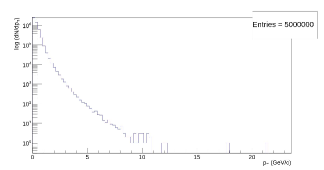
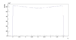
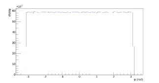
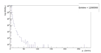
The input parameters are selected based on the criterion that they should be obtainable from laboratory measurements or derivable from other measured quantities. Moreover, the detectors that inspire the feature selection should be available at both the LHC and RHIC. Based on that information, the detectors responsible for the measurements would be hadronic and electromagnetic calorimeters[6, 7], time projection chambers[8, 9], and silicon vertex detectors. These detectors are foundational and essential for particle colliders. There is an additional constraint on the parameters, which is that they must be able to be generated using the event generator Pythia 8. The distributions of the key input features for both the low- and high- sets are shown in Figure 1, illustrating the kinematic differences between the two datasets.
 |
 |
 |
 |
 |
 |
| Particle | Charge | % in low | % in high |
|---|---|---|---|
| 0 | 52.193 | 11.198 | |
| 0 | 1.791 | 8.766 | |
| 0 | 1.016 | 6.578 | |
| +1 | 20.045 | 24.708 | |
| +1 | 1.024 | 6.580 | |
| +1 | 1.812 | 8.714 | |
| 0.328 | 0.107 | ||
| 1.806 | 8.661 | ||
| 19.983 | 24.688 |
3.1 Momentum and Angular Distributions
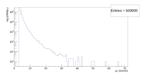
The transverse momentum distribution experiences a steep falloff consistent with a power-law spectrum at high [10]. This indicates the dominance of soft QCD processes, with most of the particles falling in the – region. Moreover, only a tiny number of particles have higher due to the scarcity of hard scattering processes. This distribution is qualitatively similar to the full momentum distribution, as the transverse momentum represents a component of the total momentum. The logarithmic scale was chosen to highlight the tail of the curve and the large dynamic range of particle transverse momentum values.
The pseudorapidity distribution is symmetric around zero, as expected for particles produced in the central rapidity region in symmetric proton–proton collisions[11]. The cut corresponds to a polar angle between and , avoiding regions too close to the beamline. This distribution closely matches the rapidity distribution at high momentum under the condition that . The azimuthal distribution is completely symmetric and uniform, indicating isotropic particle production. Moreover, the values of the azimuthal angle span the full range , providing full coverage around the beam axis.
3.2 Low- Particle Composition
In the low regime shown in Table 3, the most dominant particles are neutral particles, which is natural since approximately of the particles are photons. These photons are primarily produced from the decay of neutral pions via . This decay has a branching ratio of approximately [12], and is a major contributor to the photon abundance. Additionally, photons can be produced directly during collisions or as byproducts of other decays.
The second most abundant particles are the positive and negative pions, each constituting about of the particles. Their abundance is due to their low mass, making them kinematically favored in QCD interactions. Their numbers are equal due to isospin symmetry, as , , and form an isospin triplet [13]. Had the neutral pion not decayed promptly, the number of would have matched the counts, but its rapid decay into two photons effectively boosts the photon yield relative to charged pions.
Protons and neutrons, which form an isospin doublet [13], are produced in approximately equal numbers due to having similar mass and quark structure. Their overall lower production rate compared to pions is attributed to their higher mass, making their production less kinematically favorable.
Kaons, which include a strange quark or antiquark, are produced in approximately equal numbers between and as a reflection of strangeness conservation. However, strange quarks are subject to strangeness suppression [14], leading to fewer kaons compared to pions. The kaon-to-pion ratio () calculated as is consistent with typical values observed in high-energy proton-proton collisions [15].
Finally, electrons represent the least abundant particle type because they are produced via electromagnetic processes, which are less dominant compared to strong interactions in these collisions.
3.3 High- Behavior and Transitions
Compared to the low- regime, the high- momentum distribution decreases more gradually, with the falloff occurring around compared to earlier. Most particles in the high- sample have momenta between –, with rare high energy particles reaching up to – in some cases. The pseudorapidity distribution remains completely uniform and symmetric, showing no drop at . The azimuthal distribution retains its uniformity, consistent with the low- data.
The particle type and charge distributions exhibit notable shifts at high transverse momentum. Photons, previously dominant at low , now account for only about of the total. While the decay process still occurs, the resulting photons often fall below the threshold. Consequently, the charged pion contribution rises, with and together making up about of the particles.
The kaons experience a significant boost in their production, rising from approximately to for both and . This increase is attributed to the greater availability of energy in collisions, partially overcoming strangeness suppression. Similarly, protons and neutrons also exhibit increased production due to the dominance of hard scattering and fragmentation processes at higher energies. Even at high , electrons still constitute only about of all produced particles, again highlighting the influence of strong interaction processes.
3.4 Suitability for Model Training
All previously examined kinematic features and distributions are consistent with theoretical expectations and align well with experimental observations from proton-proton collisions. The transition from a photon-dominated distribution to a more dynamic and energetic particle composition reflects the increasing influence of hard scattering and fragmentation processes. The cut focuses the analysis on the central detector region, where particle identification is most effective. Combining soft particles from the low momentum set with rarer, high-momentum particles ensures coverage of a broad range of the kinematic spectrum of proton-proton collisions. The physical validity and diversity of the combined dataset make it highly suitable for training the model to perform particle identification across a wide momentum range.
4 Neural Network Training
The neural network architecture chosen is a standard feed-forward network, specifically a multi-layer perceptron (MLP)[16]. The hidden layers use the Rectified Linear Unit (ReLU) activation function, a computationally efficient nonlinear activation function defined as[17]
| (1) |
Compared to other alternatives such as tanh or sigmoid, ReLU avoids exponentiation. This makes it suitable for handling large datasets such as those from LHC simulations.Non-linearity in hidden layers in essential in capturing complex relationships between inputs and outputs.
The output layer activation function and the loss function are closely related and therefore are discussed together. The SoftMax activation function is a well suited for multi-class classification which is the goal of the network. The function converts the values it receives from the hidden layer into a probability distribution of the classes, with the sum of probabilities being equal to one. The SoftMax function takes the form: [18]
| (2) |
where is the predicted probability, the denominator normalizes the output so that the sum of probabilities is equal to one. This predicted class corresponds to the highest output probability.
The network is trained to minimize the categorical cross-entropy loss, defined as [19]
| (3) |
where represents the true label of the class while represents the predicted probability of the class (output of the SoftMax function). is the total number of samples and is the number of classes. This function measures how close the predicted distribution is to the true distribution of class labels.
The optimizer is responsible for updating the weights of the model during training by adjusting key parameters like the learning rate. For this current setup, the Adaptive Moment Estimation (ADAM) optimizer is used [20]. It is adaptive as it adjusts the individual learning rates of each parameter. It combines the benefits of Root Mean Square Propagation(RMSProp)[21], including adaptive learning rates, with additional advantages such as bias correction and momentum, making it well-suited for the network at hand.
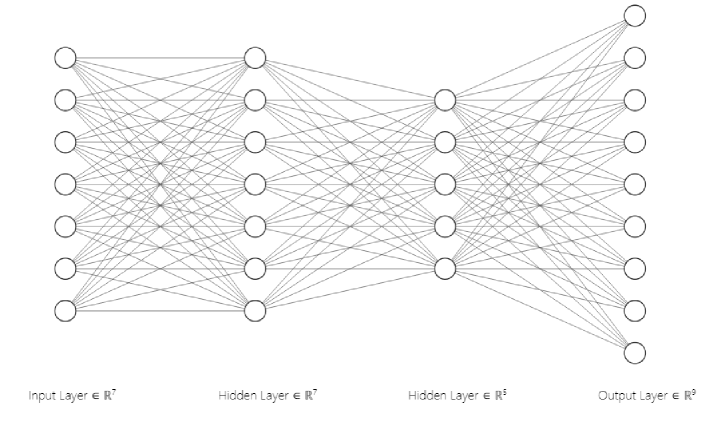
For the network’s structure, each input parameter is assigned to one neuron in the input layer; therefore, the input layer has seven neurons. The number of hidden layers depends on the complexity of the task, but having two or more makes the network a deep neural network. Deep neural networks are suitable for tasks where standard methods struggle, due to their ability to capture complex patterns. The number of neurons in the hidden layer has a wide range of integer values depending on the application. However, a good starting point is having an equal number of neurons as the input layer. This network underwent many different iterations before settling on the final structure. The initial structure was 7 neurons in both hidden layers; however, to reduce overfitting, the number of neurons was reduced to 5 in the second hidden layer. Finally, the output layer uses a SoftMax activation function, where each neuron represents the probability of a class. Since there are nine particle types, the output layer contains nine neurons. Figure 2 shows a schematic representation of the network.
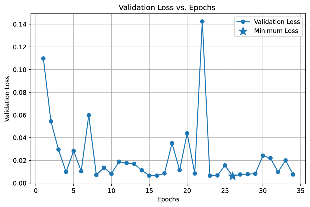
The network was trained for 34 epochs with a batch size of 128, taking an average of 41.5 seconds per epoch and about 23.5 minutes to train. The chosen regularization method is early stopping[22] with a patience value of 8. The model continues iterating until there are no improvements in validation loss for 8 consecutive epochs. Afterwards, the model restores the weights from the epoch with the lowest validation loss. This training technique improves in generalization and reduces overfitting on future test sets.
The dataset is split into three parts: training, validation, and test sets. The training set is used by the model to learn the relationships and patterns between inputs and outputs. The model iterates over the training data for 34 epochs. During training, the model receives the inputs and the true label or identification of the particle to learn the mapping between the input parameters and the output labels.
The validation consists of examples which the model hasn’t seen. It is used after each epoch to check overall how it generalizes to unseen data. The validation set is crucial in guiding and improving the performance of the model and avoiding issues such as overfitting, where the model performs well in training but fails generalizing to new examples.
The test set is used to assess the overall performance of the model after applying all the improvements and tuning during training. It is only used once, after the model has finished training, to examine how the model performs on real unseen data.
The dataset is split into an 80% training, 10% validation, and 10% test sets. Although the 90-5-5 split is common, the 80-10-10 split was chosen to maintain a large number of examples, in this case about 5 million training examples while still having a considerable validation and test set of 620 thousand examples. Figure 3 shows the change in validation loss during training. The point of minimum loss is highlighted by a star.
For the normalization of the training data, by observing the values of all the input parameters, they all fall within manageable ranges where the minimum is (from the azimuthal angle). In terms of transverse momentum, most particles fall within a range of to , with a small number of outliers having to . Naturally, for the low momentum set without the cut, most of the generated particles are soft particles having a transverse momentum value between and . Since the values for all input parameters are within close range of each other, normalization was deemed to be unnecessary.
| Point of Comparison | Training Set | Validation Set | Test Set |
|---|---|---|---|
| Accuracy (%) | 99.47 | 99.88 | 99.88 |
| Loss | 0.0172 | 0.0061 | 0.0058 |
| Number of examples | 4,960,000 | 620,000 | 620,000 |
From Table 4, the model performs well on all three sets, having comparable accuracy above 99%. The lowest accuracy among the three is the training set, but that can be attributed to its large size while the validation and test sets represent only a small subset of the total data. This means the training set contains a broader range of high momentum events, which explains its slightly reduced accuracy.
Overall, the model has no issues generalizing to unseen data based on the high performance and low loss values for both validation and test sets. The model is subsequently tested on specific cuts of high transverse momentum subsets at both RHIC and LHC energies.
5 Test Sets Results
The model was tested on both RHIC and LHC sets at a transverse momentum greater than . The high- range was probed further by dividing them into bins with -, -, and . The data were generated with the same conditions as the high- of the training data in Table 1. The only change was setting pTHatMin=4.0 GeV for convenience and to facilitate event generation. The model was tested specifically on RHIC to verify its ability to generalize to lower center-of-mass energy, as it was trained on LHC’s . The performance results are summarized in Table 5.
| Point of Comparison | High LHC | High RHIC | 3-5 LHC | 3-5 RHIC | 5-7 LHC | 5-7 RHIC | 7+ LHC | 7+ RHIC |
|---|---|---|---|---|---|---|---|---|
| Accuracy (%) | 99.44 | 99.70 | 99.80 | 99.87 | 98.24 | 98.66 | 91.33 | 96.23 |
| Loss | 0.0291 | 0.0180 | 0.0181 | 0.0129 | 0.0716 | 0.0467 | 0.2380 | 0.1108 |
| Number of examples | 500,000 | 500,000 | 50,000 | 50,000 | 50,000 | 50,000 | 50,000 | 50,000 |
The model achieves high performance in the high transverse momentum regions, retaining an accuracy above 91% for all test sets at both LHC and RHIC. Moreover, it performs as expected, having slightly lower accuracy as it moves into higher transverse momentum regions.
6 Discussion
The key difference between the two sets is strikingly visible at the cut, where the RHIC set has much better accuracy at 96.23% compared to 91.33% of the LHC set. This difference can be explained by the training of the model and the nature of the LHC set. The model has been trained on the LHC set at , which means that the particles are much more energetic overall, with momentum ranges that are much higher than RHIC, especially at the transverse momentum range of . The performance of the model on different center of mass energies can be better understood by comparing the transverse momentum distributions in Figure 4.
A dataset with the condition of includes a lot of high momentum particles, but relatively few in the region, which contributes to the drop in accuracy for LHC. For any generated set, most of the particles produced have the lowest possible energy and momentum, which corresponds to for the training set and for test set.
 |
 |
| (a) LHC distribution | (b) RHIC distribution |
7 Conclusion
This paper demonstrates the ability of a fundamentally simple deep neural network trained exclusively on simulated LHC proton-proton collisions (), to generalize to RHIC data at a much lower center-of-mass energy. This generalization is achieved without any fine-tuning, weight adjustment or transfer learning. The model maintains an accuracy above 91% at all momentum cuts, even in the complex region. For the RHIC set under the same conditions, it achieves an accuracy of 96.23%, which is quite notable as the model was not trained on any examples. The observed difference in the model’s performance is consistent with expectations, given the higher kinematic reach of the LHC. The ability of the model to generalize seamlessly to a lower center-of-mass energy highlights its robustness and suggests that it captures the underlying physics rather than overfitting to the kinematics of each regime.
These findings open the door to applying experimental simulation models in different energy domains beyond their original ones, especially in scenarios where training data is limited or simply unavailable. Future work will focus on introducing more detector-level features and employing more sophisticated network architectures, such as combined networks to handle the noisy nature of real experimental data.
8 References
References
- [1] Alexander Radovic, Mike Williams, Rousseau, et al. Machine learning at the energy and intensity frontiers of particle physics. Nature, 560(7716):41–48, 2018.
- [2] Dan Guest, Kyle Cranmer, and Daniel Whiteson. Deep Learning and its Application to LHC Physics. Ann. Rev. Nucl. Part. Sci., 68:161–181, 2018.
- [3] Dawit Belayneh, Federico Carminati, Amir Farbin, et al. Calorimetry with deep learning: particle simulation and reconstruction for collider physics. The European Physical Journal C, 80:688, 2020.
- [4] S. Acharya, D. Adamová, A. Adler, et al. Production of light-flavor hadrons in pp collisions at and . European Physical Journal C, 81, 3 2021.
- [5] T. Sjöstrand, S. Ask, J. R. Christiansen, R. Corke, N. Desai, P. Ilten, S. Mrenna, S. Prestel, C. O. Rasmussen, and P. Z. Skands. An introduction to PYTHIA 8.2. Computer Physics Communications, 191:159–177, 2015.
- [6] R.M. Brown and D.J.A. Cockerill. Electromagnetic calorimetry. Nuclear Instruments and Methods in Physics Research Section A: Accelerators, Spectrometers, Detectors and Associated Equipment, 666:47–79, 2012. Advanced Instrumentation.
- [7] C. W. Fabjan and F. Gianotti. Calorimetry for particle physics. Rev. Mod. Phys., 75:1243–1286, 2003.
- [8] Weilin Yu. Particle identification of the ALICE TPC via dE/dx. Nuclear Instruments and Methods in Physics Research Section A: Accelerators, Spectrometers, Detectors and Associated Equipment, 706:55–58, 2013. TRDs for the Third Millenium.
- [9] M Anderson, J Berkovitz, W Betts, et al. The STAR time projection chamber: a unique tool for studying high multiplicity events at RHIC. Nuclear Instruments and Methods in Physics Research Section A: Accelerators, Spectrometers, Detectors and Associated Equipment, 499(2):659–678, 2003. The Relativistic Heavy Ion Collider Project: RHIC and its Detectors.
- [10] J Nash and CMS Collaboration. Measurement of the double-differential inclusive jet cross section in proton–proton collisions . European Physical Journal C, 76(8), 2016.
- [11] V. Khachatryan, A.M. Sirunyan, A. Tumasyan, et al. Pseudorapidity distribution of charged hadrons in proton-proton collisions at = 13 TeV. Phys. Lett. B, 751:143–163, 2015.
- [12] Particle Data Group, R L Workman, V D Burkert, V Crede, et al. Review of Particle Physics. PTEP, 2022:083C01, 2022.
- [13] David J Griffiths. Introduction to elementary particles; 2nd rev. version. Wiley, 2008.
- [14] Hans-Joachim Drescher, Jörg Aichelin, and Klaus Werner. Strangeness suppression in proton-proton collisions. Physical Review D, 65(5), January 2002.
- [15] A.M. Sirunyan, A. Tumasyan, W. Adam, et al. Measurement of charged pion, kaon, and proton production in proton-proton collisions at TeV. Phys. Rev. D, 96(11):112003, 2017.
- [16] David E. Rumelhart, Geoffrey E. Hinton, and Ronald J. Williams. Learning representations by back-propagating errors. Nature, 323(6088):533–536, Oct 1986.
- [17] Vladimír Kunc and Jiří Kléma. Three decades of activations: A comprehensive survey of 400 activation functions for neural networks, 2024.
- [18] Chigozie Nwankpa, Winifred Ijomah, Anthony Gachagan, et al. Activation functions: Comparison of trends in practice and research for deep learning, 2018.
- [19] Maikel Kerkhof, Lichao Wu, Guilherme Perin, et al. No (good) loss no gain: systematic evaluation of loss functions in deep learning-based side-channel analysis. Journal of Cryptographic Engineering, 13(3):311–324, 2023.
- [20] Diederik P. Kingma and Jimmy Ba. Adam: A method for stochastic optimization, 2017.
- [21] Sebastian Ruder. An overview of gradient descent optimization algorithms, 2017.
- [22] Lutz Prechelt. Early Stopping — But When?, pages 53–67. Springer Berlin Heidelberg, Berlin, Heidelberg, 2012.
- [23] A. Adare, S. Afanasiev, C Aidala, et al. Identified charged hadron production in collisions at and 62.4 GeV. Phys. Rev. C, 83:064903, 2011.