Heisenberg limit in phase measurements: the threshold detection approach
Abstract
We analyze the fundamental sensitivity limits, achievable by the standard (single- and two-arm) optical interferometers using the Gaussian (squeezed coherent) quantum states of the probing light. We consider two types of the measurements of the output light — the standard homodyne measurement and the non-linear threshold measurement [Helstrom, “Quantum detection and estimation theory” (1976)]. The latter one allow to recover in one-shot measurement the phase information carried out by the second momenta of the quadrature amplitudes of the output light, providing the sensitivity saturating the Quantum Cramer-Rao bound.
We show that in all considered cases, the Heisenberg scaling for the phase measurement error can be achieved, where is a numerical prefactor and is the mean photon number. The specific value of the prefactor depends on the interferometer topology, the measurement type, and the quantum state of the probing light. The smaller it is, the more narrow is the range of the values of where the sensitivity that close to the best one for this specific case is provided.
I Introduction
Measurement of the phase of light using optical interferometers is one of the key tasks of experimental physics. Sensitivity of the best modern interferometers is very high and to a major extent is limited by quantum fluctuations of the probing light, see e.g. the review papers [1, 2, 3]. In particular, if the ordinary coherent state of light is used, then the best possible sensitivity corresponds to the Shot Noise Limit (SNL), equal to
| (1) |
where is the mean square phase measurement error and is the mean photon number in the probing light. Better sensitivity, for the same value of , can be achieved by using more advanced quantum states. In particular, it was proposed in Ref. [4] to use for this purpose Gaussian quadrature-squeezed states. It was shown in that work that in the case of moderate squeezing, , where is the logarithmic squeeze factor, the measurement error can be suppressed by , giving the following squeezing-enhanced SNL:
| (2) |
The most sensitive contemporary optical interferometers, namely the laser gravitational-wave detectors, like LIGO [5] or VIRGO [6], use this approach. As a result, they can measure relative elongations of their multi-kilometer length arms with the precision of about [7].
In the case of the more exotic non-Gaussian states of light, the sensitivity could reach the Heisenberg limit (HL) [8, 9, 10]:
| (3) |
where is a numerical factor. The same result could be obtained also using Gaussian squeezed states in the case of very strong squeezing, [11].
Opposite to the well-established limits (1) and (2), the HL is still subject of discussions. Various specific forms of the HL (3) and different values of the parameter can be found in literature. The main reason for this is the absence of the unique Hermitian phase operator, canonically conjugate to the photon number operator [12]. Different workarounds allowing to overcome this issue were proposed, giving different forms of the HL. In addition, in some works the sensitivity is calculated assuming given mean photon number, while in other ones — assuming given total photon number. Reviews of the various approaches to the HL can be found in Refs. [1, 13, 14].
In Refs. [15, 16, 17], the following form of the HL was obtained using numerical optimization of the phase uncertainty for the given mean photon number :
| (4) |
In addition, it was shown in Ref. [16], that if the photon number is not very small, , then the following analytical solution to this problem can be found:
| (5) |
were being the first zero of the Airy function , and the quantum state of an oscillator (e.g. the optical mode) that allows to reach this limit is a non-Gaussian one, having, in the Fock representation, the shape close to the Airy function .
At the same time, it was shown in Ref. [11] that using Gaussian squeezed states and the standard homodyne measurement procedure, it is possible to obtain the sensitivity noticeably exceeding the limit (4):
| (6) |
This discrepancy could be explained by the fact that the bound (4) is valid for any value of . This means that it does not require any a priori information on . On the other hand, the limit (6) holds only if . This means that if the sensitivity close to the HL is required, then the a priori uncertainty of the phase must not exceed the SNL value . The role of the a priori information was explored, in particular, in Refs. [18, 19, 14]. It was shown that it indeed could significantly affect the achievable sensitivity.
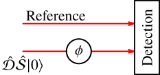
In this paper, we analyze the sensitivity limits, achievable by the standard optical interferometers and the Gaussian (squeezed coherent) quantum states. We consider two most important from the practical point of view interferometric topologies, the single-arm and the antisymmetric two-arm ones (see e.g. the review [3]). The conceptually more simple single-arm topology, see Fig. 1, directly implements measurement of the phase shift in a harmonic oscillator mode. In this case, a second beam providing the phase reference is necessary.
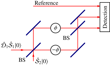
In the two-arm configuration, shown in Fig. 2 (the Mach-Zehnder topology is depicted; it is known, however, that the Michelson one is equivalent to it), the phase shifts and are introduced antisymmetrically into the first and the second arms, respectively, and both beamsplitters are the balanced 50%/50% ones. This configuration is insensitive to the common phase shift and therefore more tolerant to technical noises and drifts. Due to this reason, it is used, in particular, in the GW detectors [20].
We consider two types of the measurements of the output light. The first one, which we use as a reference point, is the well-known homodyne measurement. Its disadvantage is that it is sensitive only to the linear information on , that is the one provided by the mean values of the output quadratures of light. The second one is the non-linear threshold measurement. It was introduced in Ref. [21] (see also Sec. IV.3 of the monograph [22]) as the tool for binary discrimination between two given quantum states. Here we adapt it to the continuous measurement task. The advantage of this approach is that it allows to recover the best possible sensitivity, at least for a one given value of , while providing the explicit form of the optimal measured variable.
This paper is organized as follows. In Sec. II, we discuss the threshold measurement procedure. In Sections III and IV we calculate the sensitivity of the single-arm and double-arm interferometers, respectively, achievable by using the homodyne detection and the threshold detection. In Sec. V, we propose a possible semi-gedanken implementation of the threshold measurement, based on the quadratic () optical nonlinearity. In Sec. VI, we summarize the obtained results.
II Cramer-Rao bound and the threshold detector
We start with the well-familiar quantum Cramer-Rao bound (QCRB), see Sec. VIII.4 of the monograph [22].
Let be the density operator of an object, depending on the parameter that has to be estimated. It can be shown that the lower bound for the variance of an unbiased estimate of exists, which does not depend on the measurement procedure and has the following form:
| (7) |
where is the symmetric logarithmic derivative defined by the following equation:
| (8) |
where here and in the rest of this paper, “” means symmetrized product, that is, for any operators and ,
| (9) |
It was shown also in Ref. [22] that if the quantum state is a pure one and has the following form:
| (10) |
where
| (11) |
is a unitary displacement operator and is a Hermitian operator, then Eq. (7) can be presented in the following closed form:
| (12) |
where is the variance of in the state (10). Note that while the operator explicitly depends on , the QCRB (12) does not depend on it.
Now consider the slightly modified (adapted to the measurement of a continous variable) version of the threshold detection concept of Refs. [21, 22]. Suppose that some Hermitian operator is measured, and we are interested in the sensitivity at some given value of , for example, at (evidently, this choice does not limit the generality). Using the error propagation approach, the estimation error , corresponding to the vanishingly small values of (the threshold sensitivity) can be calculated as follows:
| (13) |
where
| (14) |
is the uncertainty of at and
| (15) |
is the gain factor. It can be shown that the minimum of the uncertainty (13) is provided by the operator satisfying the following equation:
| (16) |
It is easy to note that up to the notations, for the particular case of Eq. (8) coincides with Eq. (16). Therefore, the measurement of saturates the QCRB in this particular case, compare Eqs. (7) and (19). It is natural to expect, that this measurement should provide a good sensitivity, approaching the QCRB, albeit may be not reaching it exactly, for sufficiently small values of , satisfying the condition , where is the half-width of this good sensitivity band.
III Single-arm interferometer
The scheme.
Here we consider the single-arm interferometer shown in Fig. 1. First, we calculate the sensitivity, achievable in the case of the homodyne detection. Then we construct the explicit form of the operator measured by the threshold detector and calculate the sensitivity at . In both cases, we optimize the input state of light, assuming a given mean photon number , and express the phase measurement error in the terms of this . Finally, we calculate the sensitivity, provided by the measurement of , for the general case of , using the error propagation method.
We suppose that the probe beam is prepared in the Gaussian squeezed coherent state
| (20) |
Here is the ground state,
| (21) |
is the displacement operator (we assume without limiting the generality that the displacement parameter is real), , are, respectively, the annihilation and creation operators, and
| (22) |
is the squeeze operator with the real and non-negative squeeze factor . This choice of corresponds to the squeezed phase quadrature of the input light and therefore to the best phase sensitivity for a given , see Refs. [4, 3]. It is easy to show that the mean value and the variance of the number of quanta in the state (20) are equal to
| (23a) | |||
| (23b) | |||
Homodyne detection.
Using the Heisenberg picture, this scheme can be described by the following input/output relations:
| (24) |
where
| (25) |
is the evolution operator,
| (26) |
is the unitary phase shift operator, is the photon number operator,
| (27) |
is the rotation matrix, , are, respectively, the Hermitian amplitude and phase quadrature operators of the input field, defined by
| (28) |
and , are the corresponding operators of the output field. Note that the squeeze and displacement operations are taken into account in Eqs. (24). Therefore, the operators and corresponds to the initial vacuum field and their variances are equal to .
In the case of the small phase shift, , the phase quadrature of the output beam carries the major part of the phase information. Therefore, consider the homodyne measurement of this quadrature. Using the error propagation method, we obtain that the corresponding measurement error is equal to
| (29) |
where
| (30) |
is the variance of and
| (31) |
is the gain factor.
Threshold detector at
Consider now the threshold detector. In the Schrödinger picture, the output field of the interferometer is described by the following density operator:
| (34) |
where
| (35) |
Substituting it into Eq. (16), we obtain:
| (36) |
Consider then a set of quantum states complementing to the full orthonormal set:
| (37) |
Using this representation, Eq. (36) can be rewritten as follows:
| (38) |
This equation can be solved explicitly, giving:
| (39) |
It is easy to see from this equation, that
| (40) |
and, therefore,
| (41) |
where the variance is given by Eq. (23b).
Threshold detector at .
In order to calculate the measurement error for other values of , the explicit form of the operator is required, that is, the set and the fourth clause in Eq. (39) have to be defined explicitly. In principle, this can be done in infinite number of ways. The sensitivity at is fully defined by Eq.(39) and therefore does not depend on this choice, but the sensitivity at other values of could depend. In this paper, we consider a simple bilinear in , form of that, in principle, could be implemented in an experiment, see Sec. V.
As the natural orthonormal extension of the state (20), we consider the set of squeezed and displaced Fock states:
| (44) |
where the operators and are still given by Eqs. (21) and , respectively. In this case, using the well-known properties of the displacement and squeeze operators (21) and (22):
| (45a) | |||
| (45b) | |||
we obtain that
| (46) |
and, correspondingly,
| (47) |
where
| (48) |
As a result, Eq. (39) takes the following form:
| (49) |
A possible form of that satisfies Eq. (49) for all is the following:
| (50) |
where is an arbitrary Hermitian operator. In this paper, we consider the simplest case of .
Rolling back the squeeze and displacement operators, we obtain:
| (51) |
In the Heisenberg picture, the value of this operator at the output of the interferometer is equal to
| (52) |
see Eqs. (24).
Now we are in position to calculate the phase measurement error for all values of , using the error propagation method. We assume the same value of that gives the best possible sensitivity at , see Eq. (42). In this case, it follows from Eqs. (23a), (24), and (52) that the mean value and the variance of are equal to
| (53a) | |||
| (53b) | |||
Therefore,
| (54) |
where
| (55) |
is the gain factor.
IV Two-arm interferometer
The scheme.
In this section, we adapt the analysis of the previous section to the antisymmetric two-arm interferometer shown in Fig. 2. Following Refs. [4, 23], we assume that the squeezed coherent state is injected into the first (bright) input port, and the squeezed vacuum state — into the second (dark) input port. This combinations gives the equal values of the mean optical power in two arms. We assume also that the interferometer is tuned in such a way that in the absence of the phase signal (), both input states are reproduced at the respective bright and dark output ports (the dark fringe regime).
The corresponding two-mode input wave function is the following:
| (56) |
Here is the two-mode ground state,
| (57) |
is the displacement operator of the first (bright) input mode,
| (58a) | |||
| (58b) | |||
are, respectively, the squeeze operators of the first and the second modes, and and are the corresponding creation and annihilation operators of the input field (before the first beamsplitter). Similar to the single-arm case, we assume that the parameters , and are real (see also Ref. [3]).
We assume that the both beamsplitters are described by the following reflectivity/transmissivity matrix:
| (59) |
In this case, the annihilation operators for the intracavity fields (before the phase shifts) are equal to
| (60) |
For our calculations, we need the mean value of the sum photon number in the two arm
| (61) |
as well as the variance of the differential photon number
| (62) |
It is easy to show that this variance is equal to
| (63) |
Homodyne detector.
The input/output relations for the two-arm interferometer are the following, see again Ref. [3]:
| (64a) | |||
| (64b) | |||
where
| (65) |
is the two-mode evolution operator,
| (66) |
is the two-mode phase shift operator, is again the phase rotation matrix (27), , are the amplitude and phase quadrature operators of the input fields, defined by
| (67) |
and , are the corresponding operators of the output fields.
Similar to the single-arm scheme [compare Eqs. (24) and (64a)], we consider the homodyne measurement of the quadrature . In this case,
| (68) |
where is the variance of the measured quadrature and is the gain factor that again is equal to (31).
Let us minimize now Eq. (68) in under the condition (61) at the best sensitivity point of . In order to avoid over-cluttering the equations, we consider in more detail two most interesting particular cases: the canonical single-squeezed case of , see Ref. [4], and the anti-symmetrically double-squeezed one of . The evident third option is the symmetrically double-squeezed one, . However, calculations show that it provides the results similar to the considered in Sec. III single-arm case, but slightly inferior to it. Therefore, we do not include it in our consideration. The QCRB for this configuration was calculated in Ref. [24].
In the second case, correspondingly,
| (72) | |||
| (73) |
and
| (74) |
Threshold detector.
In the App. A, the analysis of the threshold detector, provided in Sec. III, is adapted to the two-mode case. In particular, it is shown there that the phase measurement error at is equal to
| (75) |
Let us minimize this value under the condition (61) for the same two particular cases that were considered for the homodyne measurement, namely and . If , then the minimum is provided by
| (76) |
and is equal to
| (77) |
In the second case, correspondingly,
| (78) |
and
| (79) |
The possible explicit form of is developed is App. A using the same approach as in the previous (single-arm) case. The result is the following:
| (80) |
Correspondingly, the value of this operator at the output of the interferometer is equal to
| (81) |
Consider again the particular cases of and . In the first one, in order to simplify the equations, we assume that and . The corresponding values of the gain factor and the variance of are calculated in App. A, see Eqs. (110). Substituting the optimization condition (76) into these equations, we obtain that
| (82) |
V Possible implementation of the threshold detection
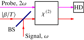
The goal of this section is to show that the measurement of in principle can be implemented using the quadratic () optical nonlinearity. The correponding scheme is shown in Fig. 3.
Omitting for brevity the subscripts “out”, the operator (52) can be presented as follows:
| (83) |
where and are the real -numbers. Apply to the displacement operator , where
| (84) |
This linear transformation can be easily implemented by mixing the measured field with the strong coherent one, using a non-symmetric beamsplitter (BS in Fig. (3)) with the amplitude transmissivity . Taking into account that
| (85) |
we obtain:
| (86) |
Below, we omit for brevity the factor and consider measurement of the operator
| (87) |
Suppose that the output light of the interferometer interacts with another (probe) mode by means of the second order optical nonlinearity, see the block in Fig. 3. This interaction is described (in the rotating wave picture) by the Hamiltonian
| (88) |
where
| (89) |
is the annihilation operator of the probe mode. The corresponding Heisenberg equation of motion for is the following:
| (90) |
Now suppose that the interaction time is short:
| (91) |
In this case, keeping only linear in terms in the solution to this equation, we obtain:
| (92) |
where is the value of after the interaction. Therefore, measurement of allows to obtain the information on with the precision, depending on the initial uncertainty of . In principle, preparing the probe mode in a highly squeezed state with , it is possible to measure and therefore with arbitrary high precision.
VI Discussion
| HD | TD | |||
|---|---|---|---|---|
| Single-arm | ||||
| Two-arm, | ||||
| Two-arm, | ||||
In the most important from the practical point of view case of the small signal phase shift , the sensitivity limits (33), (54), (71), (74), and (82), calculated in Sections III and IV, can be presented in the following unified form:
| (93) |
where is the value of the measurement error at the best sensitivity point of and is the half-width at half minimum (HWHM) of the range as of values of within which the measurement error does not exceed .
The factor allows to some extent to take into account the a priori information on the phase. If the a priori distribution fits into the range , then the resulting measurement error can be approximated by . In the opposite case, however, the more sophisticated Bayesian or maximum likelood approaches should be used.
The corresponding values of and are presented in Table 1. It can be seen that in all cases, the HL scaling can be achieved, but with different numerical factors. The best sensitivity at is provided by the single-arm interferometer combined with the threshold detection. At the same time, the single-arm interferometer is characterized by the most narrow range of the good sensitivity, , both for the homodyne and threshold detection cases.
Actually, these two features stem from the same origin, namely the strongly enhanced by squeezing amplitude quadrature of the input light , which appears in the phase quadrature of the output light if , see Eq. (24). This leads to the sharp increase of the variance with the increase of , limiting the value of , see Eq. (30). At the same time, this means also that carries information on that can be retrieved by some non-linear measurement, in particular, by the threshold detector. It is interesting that the optimization procedure prefers this information to the linear one, setting the value of the classical amplitude equal to zero, see Eq. (42). As a result, the threshold detector provides smaller by value of in comparison with the linear homodyne detector.
In the single-squeezed () two-arm interferometer case, the amplitude quadrature of the input light of the first mode appears in the measured quadrature , see Eq. (64a). In principle, the above consideration is valid in this case too. However, the variance of now is much smaller — it corresponds to the vacuum state, see Eq. (69). Therefore, both discussed above effects are much less pronounced. The good sensitivity range now scales as , but the threshold detector provides only marginal advantage in the sensitivity in comparison with the homodyne one.
Finally, in the double-squeezed case of , the variance of does not depend on at all, see Eq. (72). As a result, the non-linear term in vanishes and the threshold detection scheme reduces to the ordinary homodyne measurement. The good sensitivity range in this case is the broadest one, . At the same time, the value of is times bigger than in the previous case. This feature can be attributed to the additional term in the expression (61) for the mean number of quanta that leads to the smaller value of for the same values of and . It is worth noting that the corresponding HL prefactor is still smaller than of Refs. [15, 16, 17], despite the exotic non-Gaussian states considered in that works.
Appendix A Threshold detection in the two-arm interferometer case
In the two-arm interferometer case, Eqs. (34) and (36) take the following form:
| (94) | |||
| (95) |
where
| (96) |
Let the states , where , complement to the two-dimensional full orthonormal set:
| (97) |
Using this representation, Eq. (95) can be solved explicitly:
| (98) |
It follows from this solution that
| (99) |
As a result, we obtain Eq. (75).
Let us construct now a possible explicit form of . The two-dimensional analog of the states (44) is the following:
| (100) |
where
| (101) |
the operators , are given by Eqs. (57) and , and are the two-dimensional Fock states. Correspondingly, Eq. (98) gives:
| (102) |
where
| (103) | |||
| (104) |
Let and . In this case,
| (110a) | |||
| (110b) | |||
Acknowledgements.
This work of D.S., V.L., B.N., and F.K. was supported by the Theoretical Physics and Mathematics Advancement Foundation “BASIS” Grant #23-1-1-39-1.References
- Demkowicz-Dobrzanski et al. [2015] R. Demkowicz-Dobrzanski, M. Jarzyna, and J. Kolodynski, Chapter four - quantum limits in optical interferometry, Progress in Optics 60, 345 (2015).
- Andersen et al. [2019] U. L. Andersen, O. Glöckl, T. Gehring, and G. Leuchs, Quantum interferometry with gaussian states, in Quantum Information (John Wiley & Sons, Ltd, 2019) Chap. 35, pp. 777–798, https://onlinelibrary.wiley.com/doi/pdf/10.1002/9783527805785.ch35 .
- Salykina and Khalili [2023] D. Salykina and F. Khalili, Sensitivity of quantum-enhanced interferometers, Symmetry 15, 774 (2023).
- Caves [1981] C. M. Caves, Quantum-mechanical noise in an interferometer, Phys. Rev. D 23, 1693 (1981).
- [5] https://www.ligo.org.
- [6] http://www.virgo-gw.eu.
- Wenxuan Jia et all [2024] Wenxuan Jia et all, Squeezing the quantum noise of a gravitational-wave detector below the standard quantum limit, Science 385, 1318 (2024), https://www.science.org/doi/pdf/10.1126/science.ado8069 .
- Holland and Burnett [1993] M. J. Holland and K. Burnett, Interferometric detection of optical phase shifts at the heisenberg limit, Phys. Rev. Lett. 71, 1355 (1993).
- Bollinger et al. [1996] J. Bollinger, W. M. Itano, D. J. Wineland, and D. J. Heinzen, Optimal frequency measurements with maximally correlated states, Phys. Rev. A 54, R4649 (1996).
- Demkowicz-Dobrzański et al. [2012] R. Demkowicz-Dobrzański, J. Kołodyński, and M. Guţă, The elusive heisenberg limit in quantum-enhanced metrology, Nature Communications 3, 1063 (2012).
- Manceau et al. [2017] M. Manceau, F. Khalili, and M. Chekhova, Improving the phase super-sensitivity of squeezing-assisted interferometers by squeeze factor unbalancing, New Journal of Physics 19, 013014 (2017).
- Carruthers and Nieto [1968] P. Carruthers and M. M. Nieto, Phase and angle variables in quantum mechanics, Rev. Mod. Phys. 40, 411 (1968).
- Barbieri [2022] M. Barbieri, Optical quantum metrology, PRX Quantum 3, 010202 (2022).
- Górecki [2023] W. Górecki, Heisenberg limit beyond quantum fisher information (2023), arXiv:2304.14370 [quant-ph] .
- Summy and Pegg [1990] G. Summy and D. Pegg, Phase optimized quantum states of light, Optics Communications 77, 75 (1990).
- Bandilla et al. [1991] A. Bandilla, H. Paul, and H. H. Ritze, Realistic quantum states of light with minimum phase uncertainty, Quantum Optics: Journal of the European Optical Society Part B 3, 267 (1991).
- Hall et al. [2012] M. J. W. Hall, D. W. Berry, M. Zwierz, and H. M. Wiseman, Universality of the heisenberg limit for estimates of random phase shifts, Phys. Rev. A 85, 041802 (2012).
- Hall and Wiseman [2012] M. J. W. Hall and H. M. Wiseman, Heisenberg-style bounds for arbitrary estimates of shift parameters including prior information, New Journal of Physics 14, 033040 (2012).
- Górecki et al. [2020] W. Górecki, R. Demkowicz-Dobrzański, H. M. Wiseman, and D. W. Berry, -corrected heisenberg limit, Phys. Rev. Lett. 124, 030501 (2020).
- J.Aasi et al [2015] J.Aasi et al, Advanced ligo, Classical and Quantum Gravity 32, 074001 (2015).
- Helstrom [1967] C. W. Helstrom, Detection theory and quantum mechanics, Information and Control 10, 254 (1967).
- Helstrom [1976] C. W. Helstrom, Quantum detection and estimation theory (Academic Press, New York, 1976) p. 309.
- Lang and Caves [2013] M. D. Lang and C. M. Caves, Optimal quantum-enhanced interferometry using a laser power source, Phys. Rev. Lett. 111, 173601 (2013).
- Lang and Caves [2014] M. D. Lang and C. M. Caves, Optimal quantum-enhanced interferometry, Phys. Rev. A 90, 025802 (2014).