Beyond $\tilde{O}(\sqrt{T})$ Constraint Violation for Online Convex Optimization with Adversarial Constraints

Abstract

We revisit the Online Convex Optimization problem with adversarial constraints (COCO) where, in each round, a learner is presented with a convex cost function and a convex constraint function, both of which may be chosen adversarially. The learner selects actions from a convex decision set in an online fashion, with the goal of minimizing both regret and the cumulative constraint violation (CCV) over a horizon of $T$ rounds. The best-known policy for this problem achieves $O(\sqrt{T})$ regret and $\tilde{O}(\sqrt{T})$ CCV. In this paper, we present a surprising improvement that achieves a significantly smaller CCV by trading it off with regret. Specifically, for any bounded convex cost and constraint functions, we propose an online policy that achieves $\tilde{O}(\sqrt{dT}+T^{\beta})$ regret and $\tilde{O}(dT^{1-\beta})$ CCV, where $d$ is the dimension of the decision set and $\beta\in[0,1]$ is a tunable parameter. We achieve this result by first considering the special case of Constrained Expert problem where the decision set is a probability simplex and the cost and constraint functions are linear. Leveraging a new adaptive small-loss regret bound, we propose an efficient policy for the Constrained Expert problem, that attains $O(\sqrt{T\ln N}+T^{\beta})$ regret and $\tilde{O}(T^{1-\beta}\ln N)$ CCV, where $N$ is the number of experts. The original problem is then reduced to the Constrained Expert problem via a covering argument. Finally, with an additional smoothness assumption, we propose an efficient gradient-based policy attaining $O(T^{\max(\nicefrac{{1}}{{2}},\beta)})$ regret and $\tilde{O}(T^{1-\beta})$ CCV.

1 Introduction

Online Convex Optimization (OCO) is a standard framework for sequential decision-making under adversarial uncertainty (Hazan, 2022). At each round $1\leq t\leq T$, a learner selects an action $x_{t}$ from a convex decision set $\mathcal{X}$ with finite diameter $D$. The environment then reveals a convex, Lipschitz continuous cost function $f_{t}:\mathcal{X}\mapsto\mathbb{R}$, and, the learner incurs a cost of $f_{t}(x_{t})$. The objective is to minimize the regret relative to the best fixed action in hindsight. For any comparator action $x^{\star}\in\mathcal{X},$ the regret is defined as:

$$\textrm{Regret}_{T}(x^{\star})=\sum_{t=1}^{T}f_{t}(x_{t})-\sum_{t=1}^{T}f_{t}(x^{\star}).$$ (1)

The worst-case regret is defined to be $\sup_{x^{\star}\in\mathcal{X}}\textrm{Regret}_{T}(x^{\star})$. It is well-known that simple algorithms such as Online Mirror Descent (OMD) attain an $O(\sqrt{T})$ worst-case regret, which is also minimax optimal (Hazan, 2022).

Online Convex Optimization with adversarial constraints (COCO) generalizes the standard OCO framework and underpins a variety of emerging applications, including AI safety (Amodei et al., 2016; Sun et al., 2017), fair allocation (Sinha, 2023), online ad markets with budget constraints (Liakopoulos et al., 2019), and multi-task learning (Ruder, 2017; Dekel et al., 2006). In this problem, on each round $1\leq t\leq T,$ the learner selects an action $x_{t}$ from a convex decision set $\mathcal{X}$ with diameter $D$. The adversary then reveals two convex functions - a cost function $f_{t}:\mathcal{X}\mapsto\mathbb{R}$ and a non-negative constraint penalty function $g_{t}:\mathcal{X}\mapsto\mathbb{R}.$ For simplicity, we make the following mild assumption:

Assumption 1 (Bounded cost and constraints).

The cost and constraint penalty functions are bounded. Without loss of generality, via appropriate translation and scaling, we assume that $0\leq f_{t},g_{t}\leq 1,\forall t.$

See Section 7.1 in the Appendix for a brief discussion on Assumption 1. The constraint penalty function $g_{t}$ corresponds to a constraint of the form $h_{t}(x)\leq 0$ where we define $g_{t}(x)\equiv\max(0,h_{t}(x)).$ Thus, $g_{t}(x_{t})$ quantifies the penalty incurred by the learner for violating the hard constraint at round $t$. Hence, if an action $x^{\star}$ satisfies $g_{t}(x^{\star})=0,\forall t$, then it is feasible throughout the horizon. To measure long-term constraint violation of a policy, we define Cumulative Constraint Violation (CCV) as:

$$\textrm{CCV}_{T}=\sum_{t=1}^{T}g_{t}(x_{t}).$$ (2)

Since the constraint on each round is revealed after the learner selects action - and may be chosen adversarially - it is generally impossible for an online policy to satisfy the constraints on every round. Therefore, to ensure the problem is well-posed, one must impose some restrictions on the constraint functions (Mannor et al., 2009). In the COCO literature, the following feasibility assumption is universally made (Sinha and Vaze, 2024; Guo et al., 2022; Neely and Yu, 2017; Yuan and Lamperski, 2018; Yi et al., 2021).

Define the feasible set $\mathcal{X}^{\star}$ to be the subset of actions that satisfy all constraints across all rounds:

$$\mathcal{X}^{\star}=\{x\in\mathcal{X}:g_{t}(x)=0,~\forall t\geq 1\}.$$ (3)

Assumption 2 (Feasibility).

The feasible set is non-empty, i.e., $\mathcal{X}^{\star}\neq\emptyset.$

In the COCO problem, the regret of any policy is computed relative to the best feasible action in hindsight, i.e.,

$$\textrm{Regret}_{T}=\sup_{x^{\star}\in\mathcal{X}^{\star}}\textrm{Regret}_{T}(x^{\star}).$$ (4)

Goal:

The objective in the COCO framework is to design an online policy that achieves both low regret and low CCV over a time horizon of length $T$. In this work, our primary focus is on minimizing CCV as much as possible, while ensuring that the regret still remains sublinear. This trade-off is particularly important in safety-critical applications, such as autonomous driving, where minimizing constraint violation (e.g., safety breaches) is more critical than minimizing regret (e.g., optimizing fuel/battery consumption).

Background and Our Contribution

Recently, Sinha and Vaze (2024) proposed a gradient-based online policy for the COCO problem, which simultaneously achieves $O(\sqrt{{T}})$ regret and $\tilde{O}(\sqrt{T})$ CCV. They also established the tightness of their bounds in the high-dimensional regime, where the dimension $d$ of the decision set $\mathcal{X}$ is at least $T.$ It is well-known that even in the standard OCO problem, where $g_{t}=0,\forall t$, the regret is lower bounded by $\Omega(\sqrt{T}),$ even for $d=1$ (Hazan, 2022, Theorem 3.2). Thus the $O(\sqrt{T})$ regret bound cannot be improved. However, the natural question of whether one can achieve a CCV bound strictly smaller than $\tilde{O}(\sqrt{T})$ in the fixed-dimensional setting or under additional assumptions (e.g., smoothness) was left open.

Our main contribution in this paper is to affirmatively answer this question. In particular, we show that in the fixed-dimensional setting where $d\ll T,$ it is possible to achieve significantly smaller cumulative constraint violation (CCV) while appropriately trading off the regret. Furthermore, when the cost and constraint functions are both smooth and convex, we show that a first-order policy can achieve improved guarantees irrespective of the dimension of the decision set. A summary of our results is provided in Table 1. As a corollary, we conclude that with $\beta=1,$ the proposed policy achieves $O(\ln T)$ CCV in the special case of Online Constraint Satisfaction (OCS) problem when all cost functions are zero and the only goal is to satisfy the constraints (Sinha and Vaze, 2024).

A key technical ingredient in our analysis is the use of small-loss regret bounds, also known as $L^{\star}$ bounds in the literature (Cesa-Bianchi and Lugosi, 2006; Orabona, 2019). These bounds yield improved regret guarantees beyond the standard $O(\sqrt{T})$ bounds when the static comparator accumulates a small cumulative loss. In Section 3, we first consider the special case of Constrained Expert problem where the decision set is an $N$-dimensional simplex and the cost and constraint functions are linear. We propose a new adaptive Hedge policy that yields a small-loss regret bound for unbounded losses. In Section 4, the general problem is reduced to the Constrained Expert problem via a covering argument. Section 5 gives an efficient first-order policy with improved bounds for smooth and convex functions. Due to space constraints, experimental results have been reported in Section 7.6 in the Appendix.

Summary of the results for the constrained OCO problem Reference Regret CCV Complexity Setting Jenatton et al. (2016) $O(T^{\max(\beta,1-\beta)})$ $O(T^{1-\beta/2})$ Projection Time-invariant constraints Sun et al. (2017) $O(\sqrt{T})$ $O(T^{\nicefrac{{3}}{{4}}})$ Bregman Proj. - Neely and Yu (2017) $O(\sqrt{T})$ $O(\sqrt{T})$ Conv-OPT Slater condition Yuan and Lamperski (2018) $O(T^{\max(\beta,1-\beta)})$ $O(T^{1-\beta/2})$ Projection Time-invariant constraints Yu and Neely (2020) $O(\sqrt{T})$ $O(1)$ Conv-OPT Slater & Time-invariant constraints Yi et al. (2021) $O(T^{\max(\beta,1-\beta)})$ $O(T^{(1-\beta)/2})$ Conv-OPT Time-invariant constraints Guo et al. (2022) $O(\sqrt{T})$ $O(T^{\nicefrac{{3}}{{4}}})$ Conv-OPT - Yi et al. (2023) $O(T^{\max(\beta,1-\beta)})$ $O(T^{1-\beta/2})$ Conv-OPT - Sinha and Vaze (2024) $O(\sqrt{T})$ $\tilde{O}(\sqrt{T})$ Projection - This paper $O(\sqrt{T\ln N}+T^{\beta})$ $\tilde{O}(T^{1-\beta}\ln N)$ $O(N)$ Constrained Expert with $N$ experts This paper $\tilde{O}(\sqrt{dT}+T^{\beta})$ $\tilde{O}(dT^{1-\beta})$ $O(T^{d})$ $d$-dimensional decision set This paper $O(\sqrt{MT}+T^{\beta})$ $\tilde{O}(MT^{1-\beta})$ Projection $M$-smooth cost and constraints

Table 1: Summary of the results for the COCO problem. In the above table, $\beta\in[0,1]$ is a tunable parameter. Conv-OPT refers to solving a constrained convex optimization problem on each round. Projection refers to the Euclidean projection operation on the convex decision set $\mathcal{X}$.

Intuition for the results:

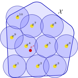
Figure 1: Schematic depicting the greedy construction of a minimal $\delta$-cover of the decision set $\mathcal{X}$. If a point $x\in\mathcal{X}$ is not covered yet, we construct a ball of radius $\delta$ centred at $x$ and include the point $x$ in the $\delta$-cover. The process continues till the entire set $\mathcal{X}$ is covered.

The following informal argument builds intuition for why the Cumulative Constraint Violation (CCV) can indeed be reduced beyond the current-best bound of $\tilde{O}(\sqrt{T}).$ Consider the Online Constraint Satisfaction (OCS) problem (Sinha and Vaze, 2024) where all cost functions are zero, and the learner’s only objective is to minimize the CCV. To solve this problem, consider a minimal $\delta$-cover of the decision set $\mathcal{X}$ with $N_{\delta}$ discrete actions. See Section 4 for a formal definition of $\delta$-cover and Figure 1 in the Appendix for a schematic. Each discrete action $x^{i}$ incurs a constraint violation of $g_{t}(x^{i})$ on round $t$. Suppose, for simplicity, that one of these actions - say, $x^{i^{\star}}$, is feasible at every round, i.e., $g_{t}(x^{i^{\star}})=0$ for all $t$ (this will be relaxed shortly). Now we run the standard Hedge algorithm on $N_{\delta}$ discrete actions with a constant learning rate $\eta=1$. Since, the action $x^{i^{\star}}$ incurs zero cost on every round, the small-loss regret bound from Eqn. (6) implies that the learner’s cumulative cost, which upper bounds the CCV, is at most $O(\log N_{\delta}).$

Finally, the above assumption of the perfect feasibility of the discrete actions can be relaxed by appealing to the Lipschitz continuity of the constraint functions and using Assumption 2. The best discrete action in hindsight then accumulates at most $O(\delta T)$ CCV. Since $N_{\delta}\sim\delta^{-d}$ for a $d$-dimensional bounded decision set (Wainwright, 2019, Lemma 5.7), plugging in these values into the bound in Eqn. (6), we obtain $\textrm{CCV}_{T}\leq O(\delta T)+O\big{(}\sqrt{\delta Td\ln\frac{1}{\delta}}+d\ln\frac{1}{\delta}\big{)}.$ Upon setting $\delta=1/T,$ we conclude that $\textrm{CCV}_{T}=O(d\ln T)$. In this paper, we generalize the above observation by exploring the trade-off between regret and CCV while taking into account the cost functions. Our result roughly says that any $(\textrm{Regret}_{T},\textrm{CCV}_{T})$ pair with $\textrm{Regret}_{T}\geq\tilde{\Theta}(\sqrt{T})$ and $\textrm{Regret}_{T}\times\textrm{CCV}_{T}=\tilde{O}(T)$ is achievable.

1.1 Prior work

Online convex optimization with constraints has been extensively studied under various modeling assumptions. Table 1 provides a summary of key results in the literature.

In the fixed-constraint setting, where $g_{t}=g$ for all $t$, Yi et al. (2021) proposed a policy that achieves $O(T^{\max(\beta,1-\beta)})$ regret and $O(T^{(1-\beta)/2})$ CCV. Under the stronger assumption of Slater’s condition, which requires the existence of a uniformly strictly feasible action $x^{\star}\in\mathcal{X}$ such that $g_{t}(x^{\star})\leq-\eta$ for some constant $\eta>0$ and all $t$, Yu and Neely (2020) showed that the CCV can be reduced to $O(1/\eta)$ while maintaining $O(\sqrt{T})$ regret.

The problem becomes significantly more challenging in the presence of time-varying adversarial constraints. Under Slater’s condition, Neely and Yu (2017) developed an algorithm achieving $O(\sqrt{T})$ regret and $O(\sqrt{T}/\eta)$ CCV. However, since Slater’s condition is quite strong, difficult to verify in practice, and leads to vacuous CCV bounds as $\eta\to 0^{+}$, recent works have focused on the general COCO setting without this assumption.

Guo et al. (2022) proposed an algorithm that needs to solve a separate offline convex optimization problem in each round, achieving $O(\sqrt{T})$ regret and $O(T^{3/4})$ CCV. Subsequently, Sinha and Vaze (2024) introduced a simpler gradient-based policy that improves the CCV bound to $\tilde{O}(\sqrt{T})$ while still maintaining $O(\sqrt{T})$ regret. More recently, Vaze and Sinha (2025) proposed an algorithm that achieves $O(\sqrt{T})$ regret and an instance-dependent CCV bound that may not scale with the time horizon. They also demonstrate that constant CCV is attainable for certain classes of constraint sets.

Separately, small-loss regret bounds, where regret scales with the cumulative loss of the benchmark rather than the time horizon, have been well studied (Cesa-Bianchi et al., 1997; Auer et al., 2002; Hazan and Kale, 2010). However, to the best of our knowledge, adaptive, scale-free variants of these small-loss bounds have not been explored prior to our work. Finally, see Neely (2010) and Xu (2023) for applications of Lyapunov drift-based techniques in stochastic network control and online learning.

2 Preliminaries: Small-Loss Regret Bound for the Expert Problem

The Prediction with Expert Advice problem, also known as the Expert problem in the literature, refers to a repeated game where, in each round $t\geq 1,$ the learner chooses a probability distribution $p_{t}\in\Delta_{N}$ over a set of $N$ experts (experts may be identified with the set of actions). After that, the adversary chooses a loss vector $l_{t}\in[0,1]^{N},$ where $l_{t}(i)$ denotes the loss for the $i$^th expert, $i\in[N]$. Consequently, the learner incurs an expected loss of $\langle l_{t},p_{t}\rangle$ in round $t.$ The full loss vector $l_{t}$ is revealed to the learner at the end of round $t.$ The learner’s objective is to choose a sequence of distributions $\{p_{t}\}_{t\geq 1}$ to minimize its cumulative regret over $T$ rounds. The Expert problem is the full-information counterpart of the Multi-armed Bandit (MAB) problem (Bubeck et al., 2012).

The Exponential Weights algorithm, also known as Hedge, is a well-known solution to the Expert problem. The Hedge algorithm selects the $i$^th expert on round $t$ with probability $p_{t}(i)$ where,

$$p_{t}(i)=\exp(-\eta\sum_{\tau=1}^{t-1}l_{\tau}(i))/Z,~i\in[N].$$ (5)

Here, $\eta>0$ is a suitably chosen learning rate and $Z$ is the normalizing constant. Hedge is known to achieve the following small-loss regret bound (Cesa-Bianchi and Lugosi, 2006, Corollary 2.4):

$$\textrm{Regret}_{T}=\tilde{L}_{T}-L_{T}(i^{\star})\leq\sqrt{2L_{T}(i^{\star})\ln N}+\ln N,$$ (6)

where $\tilde{L}_{T}=\sum_{\tau=1}^{T}\langle l_{\tau},p_{t}\rangle$ is the learner’s cumulative loss, $L_{T}(i^{\star})=\sum_{\tau=1}^{T}l_{\tau}(i^{\star})$ is the cumulative loss of a comparator arm $i^{\star}\in[N]$. The small-loss bound (6) offers a significant improvement over the standard $O(\sqrt{T})$ regret bound when the comparator’s loss is small, i.e., $L_{T}(i^{\star})=o(T)$. While the bound (6) is well-known, it assumes that that all loss values are uniformly bounded above by a known constant, typically $1$ (Cesa-Bianchi and Lugosi, 2006, Section 2.4). However, as a subroutine to our proposed algorithm, we will need to investigate problems where the loss vector on any round depends on the previous trajectory, and hence, cannot be effectively upper bounded a priori. Hence, the standard Hedge algorithm and the bound (6) cannot be used in our case.

To address this technical difficulty, Theorem 1 presents a generalized small-loss regret bound for the Expert problem that accommodates potentially unbounded losses. This bound is attained by an adaptive variant of the Hedge policy that employs a self-confident continuously variable learning rate. The full pseudocode for this adaptive Hedge policy is provided in Algorithm 3 in Appendix 7.2.

Theorem 1.

Consider the Expert problem with $N$ experts. Let $l_{t}$ be the non-negative loss vector at round $t$, and let $G_{t}$ be an upper bound to $||l_{t}||_{\infty}$ satisfying the following conditions:

1. The sequence $\{G_{t}\}_{t\geq 1}$ is monotonically non-decreasing, i.e., $G_{t}\geq G_{t-1},\forall t\geq 1.$

2. The growth of $G_{t}$ is bounded: $\max_{1\leq t\leq T}\frac{G_{t}}{G_{t-1}}\leq\gamma$ for some known constant $\gamma\geq 1.$

Then the adaptive Hedge algorithm, which selects the $i$^th expert with probability $p_{t}(i)\propto\exp(-\eta_{t}L_{t-1}(i)),\forall i,$ using an adaptive learning rate $\eta_{t}=\frac{1}{\sqrt{G_{t-1}}}\sqrt{\frac{\ln N}{\tilde{L}_{t-1}+\gamma G_{t-1}}},$ achieves the following small-loss regret bound:

$$\tilde{L}_{T}-L_{T}(i^{\star})\leq 2\gamma\sqrt{L_{T}(i^{\star})G_{T}\ln N}+7\gamma^{2}G_{T}\ln N.$$ (7)

In the above, $\tilde{L}_{t}=\sum_{\tau=1}^{t}\langle p_{\tau},l_{\tau}\rangle$ denotes the algorithm’s cumulative loss up to round $t$ and $L_{T}(i^{\star})=\sum_{\tau=1}^{T}l_{\tau}(i^{\star})$ is the cumulative loss of any comparator expert $i^{\star}\in[N]$ up to round $T.$

See Appendix 7.3 for a complete proof of Theorem 1.

Remarks: 1. The monotonicity assumption on the sequence $\{G_{t}\}_{t\geq 1}$ entails no loss of generality, since one can always define a new sequence of upper bounds as $G_{t}^{\prime}:=\max_{1\leq\tau\leq t}G_{\tau},t\geq 1,$ which is monotonic by construction.

2. Theorem 1 generalizes the standard small-loss regret bound for the Hedge algorithm, given by Eqn. (6), which assumes $G_{t}=1,\forall t\geq 1.$ In contrast, Theorem 1 makes no such uniform boundedness assumption on the sequence $\{G_{t}\}_{t\geq 1}.$

3 Constrained Expert: Simplex Decision Set, Linear Cost, and Linear Constraint functions

In this section, we focus on an important special case of the COCO problem where the cost and constraint functions are linear and the decision set is the $N-1$-dimensional simplex $\Delta_{N}$, i.e.,

$$\mathcal{X}=\left\{p\in\mathbb{R}^{N}:\sum_{i=1}^{N}p_{i}=1,p_{i}\geq 0,\forall i\right\}.$$

On each round $t,$ the learner selects a distribution $p_{t}\in\Delta_{N}$ over $N$ experts and samples an expert according to $p_{t}$. Choosing expert $i$ incurs a cost of $f_{t}(i)$ and a constraint violation of $g_{t}(i).$ Consequently, the learner incurs an expected cost of $f_{t}(p_{t})\equiv\langle f_{t},p_{t}\rangle$ and an expected constraint violation of $g_{t}(p_{t})\equiv\langle g_{t},p_{t}\rangle$ on round $t$. Both the cost vector $f_{t}$ and the constraint vector $g_{t}$ are revealed to the learner at the end of the round. The feasibility assumption (Assumption 2), specialized to this setting, implies that there exists at least one expert $i^{\star}\in[N]$ such that $g_{t}(i^{\star})=0,\forall t.$ The learner’s objective is to generate a sequence of distributions $\{p_{t}\}_{t=1}^{T}$ that minimizes both the regret and the cumulative constraint violation (CCV).

3.1 An Online Policy for the Constrained Expert Problem

Let $\Phi:\mathbb{R}\mapsto\mathbb{R}$ be a non-decreasing convex Lyapunov function, to be specified later, and $i^{\star}$ be an uniformly feasible expert with $g_{t}(i^{\star})=0,\forall t$. Let $Q(t)$ denote the cumulative constraint violation (CCV) up to round $t,$ which evolves as follows:

$$Q(t)=Q(t-1)+\langle g_{t},p_{t}\rangle.$$ (8)

We now use the regret decomposition framework introduced by Sinha and Vaze (2024) to design an online policy for the Constrained Expert problem. Using the convexity of the Lyapunov function $\Phi(\cdot),$ we have for any $1\leq t\leq T$:

$$\Phi(Q(t))-\Phi(Q(t-1)) \leq \Phi^{\prime}(Q(t))(Q(t)-Q(t-1))$$

$$\stackrel{{\scriptstyle(a)}}{{=}} \Phi^{\prime}(Q(t))\langle g_{t},p_{t}\rangle$$

$$\stackrel{{\scriptstyle(b)}}{{=}} \Phi^{\prime}(Q(t))(\langle g_{t},p_{t}\rangle-g_{t}(i^{\star})),$$

where (a) follows from Eqn. (8) and (b) uses the fact that $g_{t}(i^{\star})=0,\forall t.$ Adding the term $\langle f_{t},p_{t}\rangle-f_{t}(i^{\star})$ to both sides of the inequality, we obtain

$$\Phi(Q(t))-\Phi(Q(t-1))+(\langle f_{t},p_{t}\rangle-f_{t}(i^{\star}))$$

$$\leq\langle f_{t}+\Phi^{\prime}(Q(t))g_{t},p_{t}\rangle-(f_{t}(i^{\star})+\Phi^{\prime}(Q(t))g_{t}(i^{\star})).$$ (9)

Define the $t$^th surrogate cost function $\hat{f}_{t}:\Delta_{N}\mapsto\mathbb{R}$ to be the following linear function:

$$\hat{f}_{t}(p)\coloneqq\langle f_{t}+\Phi^{\prime}(Q(t))g_{t},p\rangle,~~t\geq 1.$$ (10)

Summing up Eqn. (3.1) for $1\leq t\leq T,$ we obtain the following regret decomposition inequality

$$\Phi(Q(T))+\textrm{Regret}_{T}(i^{\star})\leq\Phi(Q(0))+\textrm{Regret}^{\prime}_{T}(i^{\star}).$$ (11)

In the above, $\textrm{Regret}_{T}(i^{\star})$ and $\textrm{Regret}_{T}^{\prime}(i^{\star})$ correspond to regret for the original cost functions $\{f_{t}\}_{t=1}^{T}$ and the surrogate cost functions $\{\hat{f}_{t}\}_{t=1}^{T},$ respectively, with respect to the feasible expert $i^{\star}$

Algorithm 1 presents our proposed online policy for the Constrained Expert problem. It employs the adaptive Hedge algorithm from Theorem 1 as a subroutine to minimize the RHS of Eqn. (11). Observe that the surrogate cost function $\hat{f}_{t}$ involves the term $\Phi^{\prime}(Q(t)),$ which may grow indefinitely with $t$ as $Q(t)$ grows. Hence, it is imperative to use the adaptive Hedge algorithm (Algorithm 3) which can handle unbounded losses, in contrast to the standard Hedge algorithm (5), which assumes bounded losses. The following theorem gives an upper bound to the regret and CCV achieved by Algorithm 1.

Algorithm 1 Algorithm for the Constrained Expert problem

1:Input: Number of experts $N$, Horizon length $T$, Cost vectors $\{f_{t}\}_{t=1}^{T}$ and Constraint vectors $\{g_{t}\}_{t=1}^{T},$ Tunable parameter $\beta\in[0,1].$

2:Parameter settings: $\Phi(x)=e^{\lambda x},\lambda=T^{-(1-\beta)}/(2c\ln N),c=10.$

3:Initialization: Set $Q(0)\leftarrow 0,$ Algorithm’s loss $\tilde{L}_{0}\leftarrow 0$, Loss vector of the experts $L_{0}\leftarrow\bm{0},G_{0}=1+\Phi^{\prime}(Q(0)).$

4:for each $t=1:T$ do

5:  Compute self-confident learning rate

$$\eta_{t}=\frac{1}{\sqrt{G_{t-1}}}\sqrt{\frac{\ln N}{\tilde{L}_{t-1}+\gamma G_{t-1}}}.$$ (12)

6:  Play adaptive Hedge by choosing the $i$^th expert with probability

$$p_{t}(i)=\exp(-\eta_{t}L_{t-1}(i))/\sum_{j=1}^{N}\exp(-\eta_{t}L_{t-1}(j)),~\forall i\in[N].$$

7:  Observe the vectors $f_{t},g_{t}.$ Incur a cost of $\langle f_{t},p_{t}\rangle$ and constraint violation of $\langle g_{t},p_{t}\rangle.$

8:  Update CCV and $G_{t}$:

$$Q(t)=Q(t-1)+\langle g_{t},p_{t}\rangle,~~G_{t}=1+\Phi^{\prime}(Q(t)).$$

9:  Compute the surrogate cost vector: $\hat{f}_{t}=f_{t}+\Phi^{\prime}(Q(t))g_{t}.$

10:  Update the cumulative loss of the algorithm and the cumulative loss of each expert

$$\tilde{L}_{t}=\tilde{L}_{t-1}+\langle\hat{f}_{t},p_{t}\rangle,~~L_{t}(i)=L_{t-1}(i)+\hat{f}_{t}(i),~~i\in[N]$$

11:end for each

Theorem 2.

Suppose Algorithm 1 is run with the following parameter settings: $\Phi(x)=e^{\lambda x},$ where $\lambda=T^{-(1-\beta)}/(2c\ln N),c=10$ and $\beta\in[0,1]$ is a tunable parameter. Then Algorithm 1 achieves the following Regret and CCV bounds:

$$\textrm{Regret}_{T}(i^{\star})=O(\sqrt{T\ln N}+T^{\beta}+\ln N),~\textrm{CCV}_{T}=O(T^{1-\beta}\ln N\ln T).$$

In particular, if $f_{t}=0,\forall t,$ upon setting $\beta=1,$ we obtain $\textrm{CCV}_{T}=O(\ln N\ln T).$

3.2 Proof of Theorem 2

Define the sequence $G_{t}\equiv 1+\Phi^{\prime}(Q(t)),t\geq 0,$ where the Lyapunov function $\Phi(\cdot)$ is chosen as specified in the statement of Theorem 2. From the definition of the surrogate costs (Eqn. (10)), it follows that $G_{t}$ is an upper bound to the maximum component of the surrogate cost vector:

$$||\hat{f}_{t}||_{\infty}\leq||f_{t}||_{\infty}+\Phi^{\prime}(Q(t))||g_{t}||_{\infty}\leq 1+\Phi^{\prime}(Q(t))=G_{t},\forall t.$$

Since $Q(t)$ is non-decreasing in $t$ and the function $\Phi(\cdot)$ is convex, it follows that the sequence $\{G_{t}\}_{t\geq 1}$ is also non-decreasing. Furthermore, Lemma 2 in the Appendix establishes that the ratio of successive terms in the ${G_{t}}$ sequence is uniformly bounded: $\max_{1\leq t\leq T}\frac{G_{t}}{G_{t-1}}\leq 1.08\equiv\gamma$. Thus all conditions in Theorem 1 are satisfied and we can use the small-loss regret bound (7) of the adaptive Hedge algorithm for the surrogate cost sequence $\{\hat{f}_{t}\}_{t=1}^{T}.$ Let $i^{\star}\in[N]$ be a uniformly feasible expert which has zero constraint violation on every round, i.e., $g_{t}(i^{\star})=0,\forall t.$ The cumulative surrogate cost incurred by expert $i^{\star}$ can be upper bounded as:

$$L_{T}(i^{\star})=\sum_{t=1}^{T}\big{(}f_{t}(i^{\star})+\Phi^{\prime}(Q(t))g_{t}(i^{\star})\big{)}\leq T,$$

where we have used the fact that $||f_{t}||_{\infty}\leq 1$ and $g_{t}(i^{\star})=0,\forall t\geq 1.$ Hence, using the small-loss regret bound (7), the regret for the surrogate cost functions with respect to any feasible arm $i^{\star}$ can be upper bounded as:

$$\textrm{Regret}_{T}^{\prime}(i^{\star})\leq c\sqrt{T(1+\Phi^{\prime}(Q(T))\ln N}+c(1+\Phi^{\prime}(Q(T)))\ln N,$$ (13)

where we have used the fact that $\max(2\gamma,7\gamma^{2})\leq 10=c$. Using the inequality $\sqrt{x+y}\leq\sqrt{x}+\sqrt{y}$ and substituting the bound from Eqn. (13) into the regret decomposition inequality (11), we have

$$\Phi(Q(T))+\textrm{Regret}_{T}(i^{\star}) \leq \Phi(Q(0))+c\bigg{(}\sqrt{T\ln N}+\sqrt{T\Phi^{\prime}(Q(T))\ln N}$$ (14)

$$+\Phi^{\prime}(Q(T))\ln N+\ln N\bigg{)}.$$

1. Bounding the CCV:

Using the fact that $\textrm{Regret}_{T}(i^{\star})\geq-L_{T}(i^{\star})\geq-T,$ inequality (14) yields

$$e^{\lambda Q(T)}\leq T+1+c\sqrt{T\ln N}+c\sqrt{\lambda Te^{\lambda Q(T)}\ln N}+(\lambda c\ln N)e^{\lambda Q(T)}+c\ln N.$$ (15)

Since $T\geq 1,$ our choice of the parameter $\lambda$ ensures that $\lambda c\ln N\leq\nicefrac{{1}}{{2}}.$ Using this inequality to bound the coefficient of the penultimate term on the RHS of Eqn. (15) and transposing, we obtain

$$e^{\lambda Q(T)}\leq 8\max\bigg{(}T+1,c\sqrt{T\ln N},c\sqrt{\lambda T\ln N}e^{\lambda Q(T)/2},c\ln N\bigg{)}.$$

Since the maximum value on the RHS is achieved by at least one term on the right, comparing the LHS with each term on the RHS separately and simplifying, we obtain the following bound for CCV:

$$Q(T)\leq\lambda^{-1}(c_{1}+c_{2}\ln T+c_{3}\ln\ln N),$$ (16)

where $c_{1},c_{2},c_{3}$ are universal constants.

2. Bounding the Regret:

Transposing the term $\Phi(Q(T))$ to the RHS of Eqn. (14) and using $\lambda c\ln N\leq\nicefrac{{1}}{{2}},$ we obtain

$$\textrm{Regret}_{T}(i^{\star})\leq 1+c\sqrt{T\ln N}+c\sqrt{\lambda T\ln N}e^{\lambda Q(T)/2}-\frac{1}{2}e^{\lambda Q(T)}+c\ln N.$$

Using the fact that $ax-bx^{2}\leq\frac{a^{2}}{4b},b>0$, the above inequality implies the following regret bound:

$$\textrm{Regret}_{T}(i^{\star})\leq 1+c\sqrt{T\ln N}+\frac{c^{2}}{2}\lambda T\ln N+c\ln N.$$ (17)

Substituting $\lambda=\frac{T^{-(1-\beta)}}{2c\ln N}$ into Eqns. (17) and Eqn. (16), we obtain the following regret and CCV bounds:

$$\textrm{Regret}_{T}(i^{\star})=O(\sqrt{T\ln N}+T^{\beta}+\ln N),~\textrm{CCV}_{T}=O(T^{1-\beta}\ln N\ln T).$$

$\square$

4 Convex Cost and Constraint functions

In this section, we extend our previous results to the setting where both the cost and constraint functions are convex and $G$-Lipschitz, and the decision set $\mathcal{X}$ is any convex and bounded subset of $\mathbb{R}^{d}$. We begin by recalling the notion of a $\delta$-cover of a set $\mathbb{T}$ from Wainwright (2019).

Definition 1 (Covering number).

A $\delta$-cover of a set $\mathbb{T}$ with respect to a metric $\rho$ is a set $\{\theta^{1},\theta^{2},\ldots,\theta^{N}\}\subset\mathbb{T}$ such that for each $\theta\in\mathbb{T},$ there exists some $i\in[N]$ such that $\rho(\theta,\theta^{i})\leq\delta.$ The $\delta$-covering number $N(\delta;\mathbb{T},\rho)$ is the cardinality of the smallest $\delta$-cover.

Construction:

Let $\mathcal{N}_{\delta}=\{x^{1},x^{2},\ldots,x^{N_{\delta}}\}$ be a minimal $\delta$-cover of the decision set $\mathcal{X}$ with $\delta=\nicefrac{{1}}{{T}}.$ See Figure 1 in the Appendix for a schematic. Since $\mathcal{X}$ is contained within a $d$-dimensional ball of diameter $D,$ its covering number is bounded by $N_{\delta}\leq(1+\frac{2D}{\delta})^{d}$ (Wainwright, 2019, Lemma 5.7). We now construct an instance of the Constrained Expert problem with $N_{\delta}$ experts where the $i$^th expert corresponds to the point $x^{i},i\in[N_{\delta}].$ The cost and constraint violation for round $t$ for the $i$^th expert are defined as:

$$f_{t}^{\texttt{CE}}(i)=f_{t}(x^{i}),~~g_{t}^{\texttt{CE}}(i)=(g_{t}(x^{i})-G\delta)^{+},~i\in[N_{\delta}].$$ (18)

Feasibility:

To show that the above instance of the Constrained Expert problem is feasible, consider any feasible action in the decision set $x^{\star}\in\mathcal{X}$ that satisfies $g_{t}(x^{\star})=0,\forall t.$ Let $x^{i^{\star}}$ be the nearest point in the $\delta$-cover, such that $||x^{i^{\star}}-x^{\star}||\leq\delta$. Using the $G$-Lipschitzness of the constraint function, we have

$$g_{t}^{\texttt{CE}}(i^{\star})\equiv g_{t}(x^{i^{\star}})\leq g_{t}(x^{\star})+G||x^{i^{\star}}-x^{\star}||\leq 0+G\delta.$$

Hence, from Eqn. (18), it follows that expert $i^{\star}$ is feasible as $g_{t}^{\texttt{CE}}(i^{\star})=0,\forall t.$

Algorithm:

Our strategy is summarized in Algorithm 2 where, on every round, we run Algorithm 1 on the above Constrained Expert instance. We then use the output of Algorithm 1 to select the next action as an appropriate convex combination of the points in $\mathcal{N}_{\delta}$.

Algorithm 2 Algorithm for Convex Cost and Constraints

1:Input: A minimal $\delta$-cover of $\mathcal{X}$: $\mathcal{N}_{\delta}=\{x^{1},x^{2},\ldots,x^{N_{\delta}}\}$, with $\delta=\nicefrac{{1}}{{T}}.$ Parameter $\beta\in[0,1].$

2:for each $t=1:T$ do

3:  Run Algorithm 1 on the Constrained Expert problem with $N_{\delta}$ experts where the cost and constraint vectors are given by Eqn. (18). Obtain the distribution $p_{t}$ over $\mathcal{N}_{\delta}.$

4:  Play $x_{t}=\sum_{i}p_{t}(i)x^{i}$

5:end for

Analysis:

By Eqn. (18) and Jensen’s inequality, the cost and constraint violation on any round can be upper bounded by the cost and constraint violation of the Constrained Expert instance as:

$$f_{t}(x_{t})=f_{t}(\sum_{i}p_{t}(i)x^{i})\leq\sum_{i}p_{t}(i)f_{t}(x^{i})=\langle f_{t}^{\texttt{CE}},p_{t}\rangle,$$

$$g_{t}(x_{t})=g_{t}(\sum_{i}p_{t}(i)x^{i})\leq\sum_{i}p_{t}(i)g_{t}(x^{i})\leq\langle g_{t}^{\texttt{CE}},p_{t}\rangle+G\delta.$$

In addition, using the Lipschitzness of $f_{t},$ we have $f_{t}(x^{i^{\star}})-f_{t}(x^{\star})\leq G\delta,\forall t.$ Hence, the regret and CCV of Algorithm 2 differs from that of the Constrained Expert instance by at most $G\delta T\leq G,$ which is a constant. Finally, using the fact that $\ln N_{\delta}=O(d\ln T),$ we invoke Theorem 2 to obtain the following bounds for Algorithm 2:

$$\textrm{Regret}_{T}(x^{\star})=O(\sqrt{dT\ln(T)}+T^{\beta}+d\ln T),~\textrm{CCV}_{T}=O(dT^{1-\beta}(\ln T)^{2}).$$ (19)

We summarize the result in the following theorem.

Theorem 3.

For any $\beta\in[0,1],$ there exists an online algorithm that achieves $\tilde{O}(\sqrt{dT}+T^{\beta})$ regret and $\tilde{O}(dT^{1-\beta})$ CCV for any convex, Lipschitz, and bounded cost and constraint functions over a $d$-dimensional convex and bounded decision set.

5 Smooth and Convex Cost and Constraint Functions

Although the Regret and CCV bounds, given by Theorem 3, are theoretically interesting, achieving these bounds by running Algorithm 2 with a large number of experts is practically infeasible. In this section, we propose an efficient gradient-based policy for the class of bounded smooth and convex cost and constraint functions. For this, we will need the following small-loss regret bound achieved by the Online Gradient Descent (OGD) policy for smooth and convex fumctions.

Theorem 4 (Orabona (2019), Theorem 4.25).

Let $\mathcal{X}$ be a closed non-empty convex decision set with diameter $D$. Let $l_{1},l_{2},\ldots,l_{T}$ be an arbitrary sequence of non-negative convex and $M$-smooth functions. Let $\nabla_{t}$ be the gradient of $l_{t}$ at $x_{t},t\geq 1.$ Pick any $x_{1}\in\mathcal{X},$ set the step sizes adaptively as $\eta_{t}=\frac{\sqrt{2}D}{2\sqrt{\sum_{\tau=1}^{t}||\nabla_{\tau}||_{2}^{2}}},t\geq 1,$ and consider the Online Gradient Descent (OGD) policy with adaptive step sizes which selects the next action as:

$$x_{t+1}=\textsc{Proj}_{\mathcal{X}}(x_{t}-\eta_{t}\nabla_{t}).$$ (20)

In the above, $\textsc{Proj}_{\mathcal{X}}(\cdot)$ denotes the Euclidean projection operator on to the decision set $\mathcal{X}.$ Then for all $u\in\mathcal{X},$ the following regret bound holds:

$$\textrm{Regret}_{T}(u)=\sum_{t=1}^{T}l_{t}(x_{t})-\sum_{t=1}^{T}l_{t}(u)\leq 4D\sqrt{M\sum_{t=1}^{T}l_{t}(u)}+4D^{2}M.$$

Importantly, the regret bound depends only on the cumulative loss of the comparator and not on $T.$

Algorithm and Analysis:

Let $\Phi:\mathbb{R}\mapsto\mathbb{R}$ be a non-decreasing convex Lyapunov function, $x^{\star}\in\mathcal{X}$ be a feasible action, and $Q(t)$ be the CCV up to round $t$. Using identical arguments as in the Constrained Expert problem, we have the regret decomposition inequality (c.f. Eqn. (11)):

$$\Phi(Q(T))+\textrm{Regret}_{T}(x^{\star})\leq\Phi(Q(0))+\textrm{Regret}^{\prime}_{T}(x^{\star}),$$ (21)

where $\textrm{Regret}_{T}^{\prime}$ on the RHS corresponds to the regret for the surrogate cost function sequence $\{\hat{f}_{t}\}_{t=1}^{T}$ defined as follows (c.f. Eqn. (10))

$$\hat{f}_{t}(x)\coloneqq f_{t}(x)+\Phi^{\prime}(Q(t))g_{t}(x),~x\in\mathcal{X}.$$ (22)

Clearly, all surrogate cost functions are non-negative, convex, and $M_{T}\equiv M(1+\Phi^{\prime}(Q(T))$-smooth. Our algorithm runs the OGD policy (20) on the loss sequence $\{l_{t}\equiv\hat{f}_{t}\}_{t\geq 1},$ with adaptive step sizes as given by Theorem 4. It is crucial to note that the step sizes $\{\eta_{t}\}_{t\geq 1}$, which are derived from the past gradients, do not depend on the smoothness parameter $M_{T},$ which is unknown a priori. Hence, using Theorem 4, the regret for the surrogate costs for any feasible action $x^{\star}$ can be upper bounded as:

$$\textrm{Regret}_{T}^{\prime}(x^{\star})\leq 4D\sqrt{MT(1+\Phi^{\prime}(Q(T))}+4(1+\Phi^{\prime}(Q(T))D^{2}M.$$ (23)

We have used the fact that the cumulative surrogate cost is upper bounded by $\sum_{t=1}^{T}\hat{f}_{t}(x^{\star})\leq T$ as $g_{t}(x^{\star})=0,\forall t.$ Note that the regret bound (23) derives its tightness by exploiting the feasibility of the comparator $x^{\star}$ as opposed to the standard uniform regret bounds (Orabona, 2019, Theorem 4.14), which hold for any point in the decision set. The regret bound (23) becomes algebraically identical to Eqn. (13) under the substitutions $c\leftarrow 4,\ln N\leftarrow D^{2}M$. Thus, reusing the analysis and parameter choices (including the Lyapunov function) from Theorem 2, we obtain the following result.

Theorem 5.

Let the cost and constraint functions be convex, bounded, and $M$-smooth. Let $\beta\in[0,1]$ be a tunable parameter, and define the Lyapunov function as $\Phi(x)=e^{\lambda x}$ with $\lambda=T^{-(1-\beta)}/(8D^{2}M).$ Then the Online Gradient Descent algorithm with adaptive step sizes, as defined in Theorem 4, applied to the surrogate cost functions (22), achieves the following bounds for any feasible action $x^{\star}\in\mathcal{X}$:

$$\textrm{Regret}_{T}(x^{\star})=O(D\sqrt{MT}+T^{\beta}+D^{2}M),~\textrm{CCV}_{T}=O(T^{1-\beta}M\ln T).$$

In particular, if $f_{t}=0,\forall t,$ upon setting $\beta=1,$ we obtain $\textrm{CCV}_{T}=O(M\ln T).$

6 Conclusion

We proposed online policies for the COCO problem that achieve improved cumulative constraint violation (CCV) by appropriately trading it off with regret. An important direction for future work is to design computationally efficient algorithms that attain sharper CCV guarantees in the fixed-dimensional setting. Additionally, it would be interesting to establish matching lower bounds on CCV under fixed dimensionality or smoothness assumptions.

7 Appendix

7.1 On the Boundedness Assumption

Assumption 1 implies that there exist constants $K_{f},K_{g}$ such that

$$|f_{t}(x)|\leq K_{f},~~|g_{t}(x)|\leq K_{g},\forall x\in\mathcal{X},\forall t\geq 1.$$

Since the constraint penalty function $g_{t}$ is non-negative, the above implies

$$|f_{t}(x)|\leq K_{f},~~0\leq g_{t}(x)\leq K_{g},\forall x\in\mathcal{X},\forall t\geq 1.$$

Now consider the following translated and scaled version of the cost and constraint functions:

$$\tilde{f}_{t}(x)\coloneqq\frac{f_{t}(x)}{2K_{f}}+\frac{1}{2},~~\tilde{g}_{t}(x)\coloneqq\frac{g_{t}(x)}{K_{g}},x\in\mathcal{X},t\geq 1.$$

It is easy to verify that $0\leq\tilde{f}_{t},\tilde{g}_{t}\leq 1,\forall t\geq 1.$ Hence, we can work with these modified cost and constraint functions.

P.S. With the feasibility assumption (Assumption 2), we can even obtain an explicit expression for $K_{g}$. Let $x^{\star}$ be a feasible action. Using the $G$-Lipschitzness of the function $g_{t},$ we have

$$g_{t}(x)\leq g_{t}(x^{\star})+G||x_{t}-x^{\star}||\leq 0+GD.$$

Thus we can take $K_{g}\equiv GD.$ Consequently, we only need to assume the cost functions to be bounded.

7.2 Pseudocode for the Adaptive Hedge Policy

Algorithm 3 Adaptive Hedge Algorithm for the Expert problem with Unbounded Losses

1:Input: Number of experts $N,$ Horizon length $T$, Non-negative and potentially unbounded loss vectors $\{l_{t}\}_{t=1}^{T},\gamma\geq 1.$

2:Initialization: Algorithm’s loss $\tilde{L}_{0}=0$, Losses of the experts $L_{0}=\bm{0},$ $G_{0}=1$.

3:for each $t=1:T$ do

4:  Compute self-confident learning rate

$$\eta_{t}=\frac{1}{\sqrt{G_{t-1}}}\sqrt{\frac{\ln N}{\tilde{L}_{t-1}+\gamma G_{t-1}}}.$$ (24)

5:  Play adaptive Hedge by choosing the $i$^th expert with probability

$$p_{t}(i)=\exp(-\eta_{t}L_{t-1}(i))/\sum_{j=1}^{N}\exp(-\eta_{t}L_{t-1}(j)),~\forall i\in[N].$$

6:  The loss vector $l_{t}$ is revealed to the learner

7:  Update the algorithm’s and experts’ losses

$$\tilde{L}_{t}\leftarrow\tilde{L}_{t-1}+\langle l_{t},p_{t}\rangle,~L_{t}\leftarrow L_{t-1}+l_{t}$$

8:  $G_{t}$ is an upper bound to $||l_{t}||_{\infty}$ such that $1\leq G_{t+1}/G_{t}\leq\gamma$

9:end for each

7.3 Proof of Theorem 1

Our proof adapts the arguments given in Luo [2017] for bounded losses. Let $L_{t}(i)$ denote the cumulative loss of the $i$^th expert up to round $t$, i.e., $L_{t}(i)=\sum_{\tau=1}^{t}l_{\tau}(i),i\in[N]$. Define the potential function $\Phi_{t}(\eta)=\frac{1}{\eta}\log\left(\frac{1}{N}\sum_{i=1}^{N}\exp(-\eta L_{t}(i))\right)$. We have

$$\Phi_{t}(\eta_{t})-\Phi_{t-1}(\eta_{t}) = \frac{1}{\eta_{t}}\ln\bigg{(}\frac{\sum_{i=1}^{N}\exp(-\eta_{t}L_{t}(i))}{\sum_{i=1}^{N}\exp(-\eta_{t}L_{t-1}(i))}\bigg{)}$$

$$= \frac{1}{\eta_{t}}\ln\bigg{(}\sum_{i=1}^{N}p_{t}(i)\exp(-\eta_{t}l_{t}(i))\bigg{)}$$

$$\stackrel{{\scriptstyle(a)}}{{\leq}} \frac{1}{\eta_{t}}\ln\bigg{(}\sum_{i=1}^{N}p_{t}(i)\big{(}1-\eta_{t}l_{t}(i)+\frac{\eta_{t}^{2}l_{t}^{2}(i)}{2}\big{)}\bigg{)}$$

$$= \frac{1}{\eta_{t}}\ln\bigg{(}1-\eta_{t}\langle p_{t},l_{t}\rangle+\frac{\eta_{t}^{2}}{2}\sum_{i=1}^{N}p_{t}(i)l_{t}^{2}(i)\bigg{)}$$

$$\stackrel{{\scriptstyle(b)}}{{\leq}} -\langle p_{t},l_{t}\rangle+\frac{\eta_{t}}{2}\sum_{i=1}^{N}p_{t}(i)l_{t}^{2}(i).$$

where in inequality (a), we have used the fact that $e^{-y}\leq 1-y+\frac{y^{2}}{2},\forall y\geq 0,$ and in (b), we have used the fact that $1+y\leq e^{y},\forall y\in\mathbb{R}.$ Thus we have that

$$\langle p_{t},\ell_{t}\rangle\leq\Phi_{t-1}(\eta_{t})-\Phi_{t}(\eta_{t})+\frac{\eta_{t}}{2}\sum_{i=1}^{N}p_{t}(i)\ell_{t}^{2}(i).$$ (25)

Summing the above inequality for $1\leq t\leq T$ yields

$$\tilde{L}_{T}$$

$$= \sum_{t=1}^{T}\langle p_{t},l_{t}\rangle$$

$$\leq \Phi_{0}(\eta_{1})-\Phi_{T}(\eta_{T+1})+\sum_{t=1}^{T}\frac{\eta_{t}}{2}\sum_{i=1}^{N}p_{t}(i)\ell_{t}^{2}(i)+\sum_{t=1}^{T}(\Phi_{t}(\eta_{t+1})-\Phi_{t}(\eta_{t}))$$

$$\stackrel{{\scriptstyle(a)}}{{\leq}} \frac{\ln N}{\eta_{T+1}}-\frac{1}{\eta_{T+1}}\ln\left(\exp(-\eta_{T+1}L_{T}(i^{*}))\right)+\sum_{t=1}^{T}\frac{\eta_{t}}{2}G_{t}\sum_{i=1}^{N}p_{t}(i)\ell_{t}(i)+\sum_{t=1}^{T}(\Phi_{t}(\eta_{t+1})-\Phi_{t}(\eta_{t}))$$

$$\stackrel{{\scriptstyle(b)}}{{\leq}} \sqrt{(\tilde{L}_{T}+\gamma G_{T})G_{T}\ln N}+L_{T}(i^{*})+\underbrace{\gamma\sqrt{G_{T}\ln N}\sum_{t=1}^{T}\frac{\langle p_{t},\ell_{t}\rangle}{2\sqrt{\tilde{L}_{t-1}+\gamma G_{t-1}}}}_{(A)}+\underbrace{\sum_{t=1}^{T}(\Phi_{t}(\eta_{t+1})-\Phi_{t}(\eta_{t}))}_{(B)},$$

where, in (a) we have used the fact that $||l_{t}||_{\infty}\leq G_{t},$ and in (b) we have used the expression (24) for the learning rate $\eta_{t}$ along with the fact that $G_{t}\leq\gamma G_{t-1}$ and $G_{t}\leq G_{T},\forall t.$

To bound term (A) in Eqn. (7.3), observe that

$$\tilde{L}_{t}=\tilde{L}_{t-1}+\langle p_{t},l_{t}\rangle\leq\tilde{L}_{t-1}+G_{t}\leq\tilde{L}_{t-1}+\gamma G_{t-1}.$$

Hence,

$$\sum_{t=1}^{T}\frac{\langle p_{t},\ell_{t}\rangle}{\sqrt{\tilde{L}_{t-1}+\gamma G_{t-1}}}\leq\sum_{t=1}^{T}\frac{\tilde{L}_{t}-\tilde{L}_{t-1}}{\sqrt{\tilde{L}_{t}}}\stackrel{{\scriptstyle(c)}}{{\leq}}\int_{\tilde{L}_{0}}^{\tilde{L}_{T}}\frac{dx}{\sqrt{x}}=2\sqrt{\tilde{L}_{T}},$$

where in inequality (c), we have used the monotonicity of the sequence $\{\tilde{L}_{t}\}_{t\geq 1}.$

Furthermore, it can be readily verified that the potential function $\Phi_{t}(\eta)$ is non-decreasing in $\eta$ as $\Phi_{t}^{\prime}(\eta)\geq 0$ [Luo, 2017]. Since the learning rate $\eta_{t}$ is non-increasing in $t,$ we conclude that each term in term (B) in Eqn. (7.3) is non-positive. Hence, using the inequality $\sqrt{a+b}\leq\sqrt{a}+\sqrt{b},$ from Eqn. (7.3), we have

$$\tilde{L}_{T}\leq 2\gamma\sqrt{\tilde{L}_{T}G_{T}\ln N}+L_{T}(i^{*})+G_{T}\sqrt{\gamma\ln N}.$$

In the above, we have used the fact that $\gamma\geq 1.$ Solving the above quadratic inequality using Lemma 1 below, we conclude that the adaptive Hedge policy enjoys the following small-loss regret bound for the Expert problem:

$$\tilde{L}_{T}-L_{T}(i^{\star})\leq 2\gamma\sqrt{L_{T}(i^{\star})G_{T}\ln N}+7\gamma^{2}G_{T}\ln N.$$

7.4 Proof of Helper Lemmas

Lemma 1 (A quadratic inequality).

Consider the following quadratic inequality $x^{2}\leq ax+b$, where $a\geq 0,b\geq 0.$ Then we have $x^{2}\leq a^{2}+b+a\sqrt{b}.$

Proof.

Solving the given inequality using the usual quadratic formula and the fact that $\sqrt{x+y}\leq\sqrt{x}+\sqrt{y},~x,y\geq 0,$, we have

$$x\leq\frac{a+\sqrt{a^{2}+4b}}{2}\leq\frac{a+a+2\sqrt{b}}{2}=a+\sqrt{b}.$$

Hence,

$$x^{2}\leq a(a+\sqrt{b})+b=a^{2}+b+a\sqrt{b}.$$

∎

Lemma 2 (Bounding $\gamma$).

Let $\Phi(x)=e^{\lambda x},\lambda=T^{-(1-\beta)}/(2c\ln N)$, where $c=10.$ Define $G_{t}=1+\Phi^{\prime}(Q(t)),t\geq 0$ and $\gamma\equiv\max_{1\leq t\leq T}\frac{G_{t}}{G_{t-1}}$. Then we have $\gamma\leq 1.08.$

Proof.

Since $0\leq g_{t}\leq 1,$ from Eqn. (8), we have

$$Q(t)=Q(t-1)+\langle g_{t},p_{t}\rangle\leq Q(t-1)+1.$$ (27)

Thus

$$\frac{G_{t}}{G_{t-1}} = \frac{1+\lambda e^{\lambda Q(t)}}{1+\lambda e^{\lambda Q(t-1)}}\stackrel{{\scriptstyle(a)}}{{\leq}}\frac{1+\lambda e^{\lambda}e^{\lambda Q(t-1)}}{1+\lambda e^{\lambda Q(t-1)}}\leq e^{\lambda}.$$ (28)

where in (a) we have used inequality (27). Since $N\geq 2$ and $T\geq 1,$ we have $\lambda\leq(2c\ln 2)^{-1}.$ Hence, Eqn. (28) implies that

$$\gamma\leq e^{1/(20\ln 2)}\leq 1.08.$$

∎

7.5 Construction of a Minimal $\delta$-cover of the Decision Set $\mathcal{X}$

7.6 Experiments

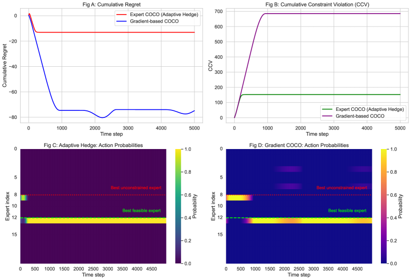
Figure 2: Comparison of the proposed adaptive Hedge-based policy (Algorithm 1) with $\beta=0.75$ and the OGD-based policy from Sinha and Vaze [2024, Algorithm 1]. (A) Regret vs. time. (B) Cumulative Constraint Violation (CCV) vs. time. (C) Selection frequency of experts under our adaptive Hedge-based policy. (D) Selection frequency of experts under the OGD-based policy. The proposed policy quickly identifies and sticks to the best feasible expert, leading to significantly lower CCV, whereas the OGD-based policy initially selects infeasible experts and takes longer to converge.

Problem instance:

We consider the Constrained Expert problem on a synthetic dataset with $N=20$ experts over a horizon of length $T=5000$. Two experts are designated as special: the best feasible expert, denoted by $\texttt{E}^{\star}$, and the best unconstrained expert, denoted by $\texttt{UE}^{\star}$. The expert $\texttt{E}^{\star}$ is feasible, with i.i.d. costs drawn from a distribution with mean $\bar{f}_{\texttt{E}^{\star}}=0.21$, and zero constraint violation on all rounds, i.e., $\bar{g}_{\texttt{E}^{\star}}=0.0$. In contrast, $\texttt{UE}^{\star}$ is infeasible, with i.i.d. costs and constraint violations having a smaller mean $\bar{f}_{\texttt{UE}^{\star}}=0.11$ and higher average constraint violation $\bar{g}_{\texttt{UE}^{\star}}=0.91$, respectively. The remaining experts incur i.i.d. random costs with mean $\bar{f}=0.41$ plus a zero-mean periodic component over time, and their constraint violations are i.i.d. with mean $\bar{g}=0.6$. Additionally, two more experts, $\texttt{DE}_{1}$ and $\texttt{DE}_{2}$, distinct from both $\texttt{E}^{\star}$ and $\texttt{UE}^{\star}$, are made feasible by setting their constraint violations to zero on all rounds. Table 2 summarizes the parameters used in the experiments. The experiments have been run on a quad-core CPU with 8 GB RAM.

Parameters for Experts Used in the Experiments Expert(s) Index Average cost Average constraint violation $\texttt{E}^{\star}$ $\#12$ $\bar{f}_{\texttt{E}^{\star}}=0.21$ $\bar{g}_{\texttt{E}^{\star}}=0.0$ $\texttt{UE}^{\star}$ $\#8$ $\bar{f}_{\texttt{E}^{\star}}=0.11$ $\bar{g}_{\texttt{E}^{\star}}=0.91$ $\texttt{DE}_{1},\texttt{DE}_{2}$ $\#3,\#6$ $\bar{f}_{\texttt{E}^{\star}}=0.41$ $\bar{g}_{\texttt{E}^{\star}}=0.0$ The rest $[20]\setminus\{3,6,8,12\}$ $\bar{f}_{\texttt{E}^{\star}}=0.41$ $\bar{g}_{\texttt{E}^{\star}}=0.6$

Table 2: Parameter settings for generating cost and constraint vectors for $N=20$ experts.

Summary of the results.

Parts (A) and (B) of Figure 2 compare the performance of our proposed adaptive Hedge-based policy (Algorithm 1) with $\beta=0.75$ with that of the Online Gradient Descent (OGD)-based policy proposed by Sinha and Vaze [2024, Algorithm 1]. From the plots, it is evident that the proposed algorithm incurs significantly lower cumulative constraint violation (CCV) while maintaining a sub-linear regret.

To gain deeper insight into the behavior of the algorithms, parts (C) and (D) of Figure 2 show the relative frequency with which each expert is selected by our algorithm and the OGD-based policy, respectively. These plots clearly demonstrate that the adaptive Hedge-based policy quickly identifies the best feasible expert and predominantly selects it thereafter. In contrast, the OGD-based policy initially incurs a substantial amount of constraint violation by frequently selecting infeasible experts. Only after a considerable number of rounds does it converge to the best feasible expert and begin exploiting it consistently.

Figure 3 illustrates the trade-off between regret and cumulative constraint violation (CCV) for different values of the tuning parameter $\beta$ in the proposed policy. As $\beta$ increases from 0.6 to 0.9, the algorithm incurs lower CCV at the expense of higher regret. This behavior aligns with the theoretical performance guarantees established in Theorem 2.

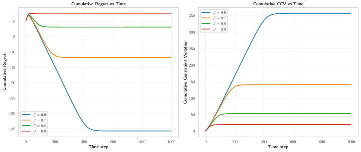
Figure 3: Performance comparison for different values of $\beta$

References

- Hazan (2022) Elad Hazan. Introduction to online convex optimization. MIT Press, 2022.
- Amodei et al. (2016) Dario Amodei, Chris Olah, Jacob Steinhardt, Paul Christiano, John Schulman, and Dan Mané. Concrete problems in ai safety. arXiv preprint arXiv:1606.06565, 2016.
- Sun et al. (2017) Wen Sun, Debadeepta Dey, and Ashish Kapoor. Safety-aware algorithms for adversarial contextual bandit. In Doina Precup and Yee Whye Teh, editors, Proceedings of the 34th International Conference on Machine Learning, volume 70 of Proceedings of Machine Learning Research, pages 3280–3288. PMLR, 06–11 Aug 2017. URL https://proceedings.mlr.press/v70/sun17a.html.
- Sinha (2023) Abhishek Sinha. BanditQ - Fair Multi-Armed Bandits with Guaranteed Rewards per Arm. arXiv preprint arXiv:2304.05219, 2023.
- Liakopoulos et al. (2019) Nikolaos Liakopoulos, Apostolos Destounis, Georgios Paschos, Thrasyvoulos Spyropoulos, and Panayotis Mertikopoulos. Cautious regret minimization: Online optimization with long-term budget constraints. In Kamalika Chaudhuri and Ruslan Salakhutdinov, editors, Proceedings of the 36th International Conference on Machine Learning, volume 97 of Proceedings of Machine Learning Research, pages 3944–3952. PMLR, 09–15 Jun 2019. URL https://proceedings.mlr.press/v97/liakopoulos19a.html.
- Ruder (2017) Sebastian Ruder. An overview of multi-task learning in deep neural networks. arXiv preprint arXiv:1706.05098, 2017.
- Dekel et al. (2006) Ofer Dekel, Philip M Long, and Yoram Singer. Online multitask learning. In International Conference on Computational Learning Theory, pages 453–467. Springer, 2006.
- Mannor et al. (2009) Shie Mannor, John N Tsitsiklis, and Jia Yuan Yu. Online learning with sample path constraints. Journal of Machine Learning Research, 10(3), 2009.
- Sinha and Vaze (2024) Abhishek Sinha and Rahul Vaze. Optimal algorithms for online convex optimization with adversarial constraints. In The Thirty-eighth Annual Conference on Neural Information Processing Systems, 2024. URL https://openreview.net/forum?id=TxffvJMnBy.
- Guo et al. (2022) Hengquan Guo, Xin Liu, Honghao Wei, and Lei Ying. Online convex optimization with hard constraints: Towards the best of two worlds and beyond. Advances in Neural Information Processing Systems, 35:36426–36439, 2022.
- Neely and Yu (2017) Michael J Neely and Hao Yu. Online convex optimization with time-varying constraints. arXiv preprint arXiv:1702.04783, 2017.
- Yuan and Lamperski (2018) Jianjun Yuan and Andrew Lamperski. Online convex optimization for cumulative constraints. Advances in Neural Information Processing Systems, 31, 2018.
- Yi et al. (2021) Xinlei Yi, Xiuxian Li, Tao Yang, Lihua Xie, Tianyou Chai, and Karl Johansson. Regret and cumulative constraint violation analysis for online convex optimization with long term constraints. In International Conference on Machine Learning, pages 11998–12008. PMLR, 2021.
- Cesa-Bianchi and Lugosi (2006) Nicolo Cesa-Bianchi and Gábor Lugosi. Prediction, learning, and games. Cambridge university press, 2006.
- Orabona (2019) Francesco Orabona. A modern introduction to online learning. arXiv preprint arXiv:1912.13213, 2019.
- Jenatton et al. (2016) Rodolphe Jenatton, Jim Huang, and Cédric Archambeau. Adaptive algorithms for online convex optimization with long-term constraints. In International Conference on Machine Learning, pages 402–411. PMLR, 2016.
- Yu and Neely (2020) Hao Yu and Michael J Neely. A low complexity algorithm with regret and constraint violations for online convex optimization with long term constraints. Journal of Machine Learning Research, 21(1):1–24, 2020.
- Yi et al. (2023) Xinlei Yi, Xiuxian Li, Tao Yang, Lihua Xie, Yiguang Hong, Tianyou Chai, and Karl H Johansson. Distributed online convex optimization with adversarial constraints: Reduced cumulative constraint violation bounds under slater’s condition. arXiv preprint arXiv:2306.00149, 2023.
- Wainwright (2019) Martin J Wainwright. High-dimensional statistics: A non-asymptotic viewpoint, volume 48. Cambridge University Press, 2019.
- Vaze and Sinha (2025) Rahul Vaze and Abhishek Sinha. ) static regret and instance dependent constraint violation for constrained online convex optimization. arXiv preprint arXiv:2502.05019, 2025.
- Cesa-Bianchi et al. (1997) Nicolo Cesa-Bianchi, Yoav Freund, David Haussler, David P Helmbold, Robert E Schapire, and Manfred K Warmuth. How to use expert advice. Journal of the ACM (JACM), 44(3):427–485, 1997.
- Auer et al. (2002) Peter Auer, Nicolo Cesa-Bianchi, and Claudio Gentile. Adaptive and self-confident on-line learning algorithms. Journal of Computer and System Sciences, 64(1):48–75, 2002.
- Hazan and Kale (2010) Elad Hazan and Satyen Kale. Extracting certainty from uncertainty: Regret bounded by variation in costs. Machine learning, 80:165–188, 2010.
- Neely (2010) Michael J Neely. Stochastic network optimization with application to communication and queueing systems. Synthesis Lectures on Communication Networks, 3(1):1–211, 2010.
- Xu (2023) Kuang Xu. Drift method: from stochastic networks to machine learning. URL: https://web. stanford. edu/˜ kuangxu/papers/driftmethod. pdf. Last visited on, 3(09), 2023.
- Bubeck et al. (2012) Sébastien Bubeck, Nicolo Cesa-Bianchi, et al. Regret analysis of stochastic and nonstochastic multi-armed bandit problems. Foundations and Trends® in Machine Learning, 5(1):1–122, 2012.
- Luo (2017) Haipeng Luo. Lecture 4. Introduction to Online Learning, 2017. https://haipeng-luo.net/courses/CSCI699/index.html.