StableMotion: Repurposing Diffusion-Based Image Priors for Motion Estimation

Abstract

We present StableMotion, a novel framework leverages knowledge (geometry and content priors) from pretrained large-scale image diffusion models to perform motion estimation, solving single-image-based image rectification tasks such as Stitched Image Rectangling (SIR) and Rolling Shutter Correction (RSC). Specifically, StableMotion framework takes text-to-image Stable Diffusion (SD) models as backbone and repurposes it into an image-to-motion estimator. To mitigate inconsistent output produced by diffusion models, we propose Adaptive Ensemble Strategy (AES) that consolidates multiple outputs into a cohesive, high-fidelity result. Additionally, we present the concept of Sampling Steps Disaster (SSD), the counterintuitive scenario where increasing the number of sampling steps can lead to poorer outcomes, which enables our framework to achieve one-step inference. StableMotion is verified on two image rectification tasks and delivers state-of-the-art performance in both, as well as showing strong generalizability. Supported by SSD, StableMotion offers a speedup of 200× compared to previous diffusion model-based methods.

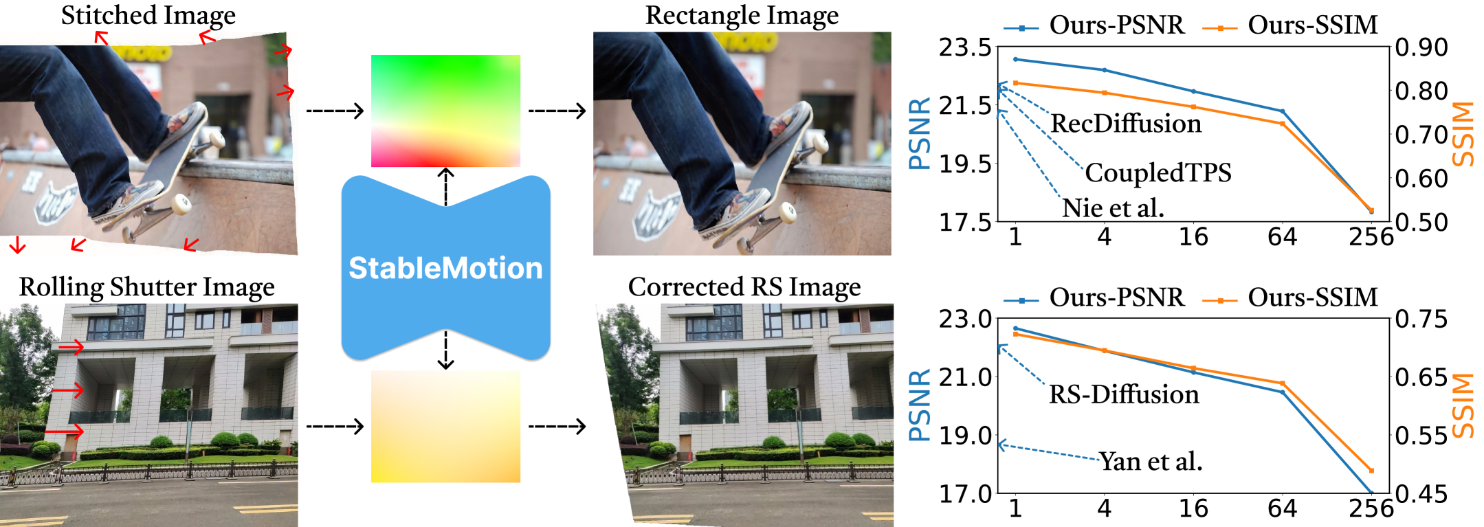
Figure 1: Two applications of the StableMotion framework, as well as the Sampling Steps Disaster (SSD).

1 Introduction

Single-image-based image rectifications, such as Stitched Image Rectangling (SIR) and Rolling Shutter Correction (RSC), have posed significant challenges. The information laid in the inputs of them is insufficient to obtain robust results, thus requiring additional information (image priors).

Stitched Image Rectangling (SIR) refers to the technique of converting stitched images with irregular edges into rectangular shapes. These stitched images are typically created by merging multiple overlapping images [39, 48, 20, 14]. He et al. [7] proposed the conception of image rectangling and presented a framework as prototype. However, it only preserves straight lines and leads to distortions in non-linear structures [53]. In the era of deep learning, Nie et al. [28] proposed a mesh-based framework, while meshes have far fewer grid points than the pixels in an image, and this low-rank representation can not fully capture complex motions, resulting in local artifacts like inconsistent boundaries or visible misalignments. Recently, Zhou et al. [52] presented a solution based on specially designed DMs. With two DMs trained from scratch and diffusion process performed in pixel-space, training and inference are computationally intensive. And for all these methods, the upper limit of model’s performance is limited by the datasets, blocking further improvements of them.

Rolling Shutter Correction (RSC) aims to rectify image distortions arise from the row-wise exposure pattern of CMOS sensors. For single-frame based rolling shutter correction, Rengarajan et al. [32] used CNN modules to estimate row-wise motion, while failing to address instances involving camera or scene movement in directions other than horizontal. Zhuang et al. [54] used depth maps as another input, while depth estimation itself is another ill-posed task. Yan et al. [45] utilized a homography mixture model, and Yang et al. [46] proposed a specially designed diffusion model. Both of them trained models from scratch, failing to solve the fundamental issue of ill-posedness, relying for high-quality datasets and numerous computing, which caps the model’s potential and making generalizing hard.

To address the inherent challenge of ill-posedness and effectively tackle these image rectification tasks, we incorporate external diffusion prior knowledge for motion estimation. We present StableMotion, a general framework based on the architecture and weights of Stable Diffusion (SD) [33], as shown in Fig. 1 (The left part. StableMotion receives different inputs, generates corresponding rectification flows, and accomplishes different tasks). Our primary motivation is derived from previous works that have leveraged SD prior knowledge in other tasks and achieved significant improvements, such as image restoration [27], depth estimation [17], etc. However, all of them are  image-to-image frameworks, suffering from unstable contents and slow inference. At the mean time, we noticed SD’s ability to perceive motion between different images [40], enabling zero-shot semantic and geometric matching. To unlock the potential of SD on motion perception, we propose StableMotion as an image-to-motion model. Specifically, a repurposed VAE is used to map images and motions between the feature and pixel spaces, and we also constrain it as a motion refiner. The UNet is adapted to estimate motion fields $F$ between the input conditional images $I_{cond}$ (i.e., stitched images for SIR and rolling shutter images for RSC) and ground truth images $I_{gt}$ (i.e., rectangle image for SIR and corrected rolling shutter image for RSC). The generated motion fields are used to perform warping operation on $I_{cond}$ to get the predicted ground truth $\hat{I}_{gt}$. Due to the generative nature of DMs, one model can produce multiple inconsistent results when performing inference on the same input. Thus, we introduce Adaptive Ensemble Strategy (AES) as an optional post-processing step to aggregate inconsistent results into a unified output.

There’s one more thing. We find that employing conditional loss to train DMs can lead to a counterintuitive phenomenon: an increase in sampling steps results in worse results (Fig 1, the right part). We introduce Sampling Steps Disaster (SSD), a theory to explain this singular phenomenon. SSD enables StableMotion to generate optimal results with one single inference step, as well as explains the choice to use fewer sampling steps in previous works [22, 52, 46].

In sum, StableMotion delivers state-of-the-art performance and strong generalizability, while significantly reduces training and inference cost. Our contributions are:

• We propose a novel framework, namely StableMotion, repurposing diffusion-based image priors in fundamental models to perform motion estimation, and verify it on two single-image-based image rectification tasks.

• We present the concept of Sampling Steps Disaster (SSD), accounting for the paradox where increasing the number of sampling steps results in poorer outcomes, and supporting StableMotion to achieve one-step inference.

• Extensive experiments demonstrate that StableMotion achieves state-of-the-art performance and generalizability on public benchmarks of both the tasks, as well as offers reduced training cost and remarkably faster inference, reaching a speed up of 200$\times$ compared to previous DM-basd methods.

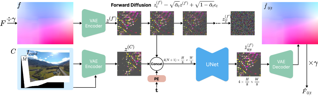
Figure 2: Repurposing from SD. Taking image rectangling as example. At each timestep, the predicted flow feature is decoded and denormalized into the pixel-space to perform warping and to construct conditional losses.

2 Related Work

2.1 Diffusion Models

Diffusion models have emerged as powerful generative models [35, 10]. These models are also formulated within score-based frameworks [37, 38], focusing on estimating the gradient of data distributions. Techniques such as classifier-guided diffusion [3, 23] and classifier-free guidance [9] offer refined control over the generative process by using auxiliary information or adjusting guidance strength. Built on them, Latent Diffusion Models (LDMs) [33] perform diffusion in the latent space, achieving an improvement in efficiency. Besides, approaches including ControlNet [50] and related methods [42, 12, 16, 24, 11, 22, 13] leverage pre-trained diffusion priors, refining the generative process to meet specific needs. Diffusion models have been widely applied to traditional tasks, such as super-resolution [26, 47] and depth-estimation [17].

2.2 Prior Based Methods

Foundational models like Stable Diffusion [33] and DeepFloyd [34] encapsulate extensive high-level semantic information, making them invaluable for a multitude of downstream tasks. These models are utilized in various ways: some gather features by feeding images into foundational models to achieve semantic/geometric matching [40, 25, 49, 8], create visual anagrams [6, 5, 2], perform 3D reconstruction [30, 43], segment images [44, 41], and classify images [21]. Concurrently, other methods directly refine these models to accomplish tasks such as depth estimation [17] and 3D geometry estimation [4]. In this work, we exploit the diffusion-based image priors for motion estimation.

2.3 Stitched Image Rectangling

He et al. [7] posed the task of image rectangling and proposed a two-stage framework. The former stage initializes an irregular mesh through seam carving [1], and the latter solves a content-preserving rectangular mesh by energy optimization. Based on that, Nie et al. [28] pioneered a deep learning approach to image rectangling by estimating mesh deformations using convolutional neural networks (CNNs). Recently, Zhou et al. [52] used specially designed diffusion models for image rectangling, employing a two-stage-cascade strategy that involves image-to-motion and image-to-image transformations. Zhang et al. [51] designed an end-to-end framework to combine image stitching and rectangling together, and Nie et al. [29] proposed a semi-supervised method for rectangling.

2.4 Rolling Shutter Correction

For single-frame rolling shutter correction, classical algorithms usually use lines and boundaries in RS images to estimate motions [31, 19]. In the deep learning era, Rengarajan et al. [32] employed CNN modules to generate row-wise motions between global shutter (GS) images and rolling shutter (RS) inputs. Zhuang et al. [54] added depth maps as another input besides the GS images, while depth estimation itself is another ill-posed task. Yan et al. [45] utilized a homography mixture model, dividing images into blocks and learning coefficients to assemble several motion bases. Recently, Yang et al. [46] proposed the first diffusion based method for single-image RSC, using a specially designed diffusion model to estimate motions in pixel space.

3 Method

We adopt the priors (i.e., pretrained weights) from existing foundation models, specifically Stable Diffusion 2.0 [33], as our backbone. The model is expected to predict a flow field $F\in\mathbb{R}^{2\times H\times W}$ representing the motion of each pixel from the condition image $I_{cond}$ towards the corresponding ground truth image ${I}_{gt}$:

$$\hat{F}=\theta(C,\epsilon),$$ (1)

where $\epsilon$ is standard Gaussian noise, and $C$ are conditions that at least contain an condition image $I_{cond}$. For SIR, $C=(I_{cond},M)$, where $I_{cond}$ refers to stitched images and $M$ is a mask indicating the blank regions in $I_{cond}$. For RSC, $C=I_{cond}$, where $I_{cond}$ represents the rolling shutter image. The predicted results can be produced via a warping operation:

$$\hat{I}_{gt}=\mathcal{W}(I_{cond},\hat{F}).$$ (2)

3.1 Background

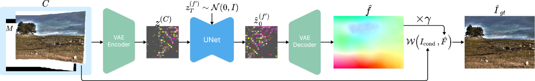
Figure 3: Overview of the inference scheme. Taking image rectangling as example. Note that the sampling process is one-step.

Classifier-free guidance.

To control the content generated by the model and balance controllability with fidelity, classifier-free guidance (CFG) [9] incorporates conditions $\mathbf{y}$ as follows:

$$p_{\theta}(\mathbf{x}_{t-1}|\mathbf{x}_{t},\mathbf{y})=\mathcal{N}\left(\mathbf{x}_{t-1};\mu_{\theta}\left(\mathbf{x}_{t},t,\mathbf{y}\right),\sigma_{t}^{2}\mathbf{I}\right).$$ (3)

CFG theoretically requires two diffusion outputs, one conditional and one unconditional. Joint training is usually applied by randomly setting the condition $y$ to a null condition $\phi$ with some probability $p_{y}$, and sampling process is a linear combination of conditional and unconditional predictions:

$$\tilde{\mu}_{\theta}\left(\mathbf{z}_{\lambda},\mathbf{y}\right)=(1+w)\mu_{\theta}\left(\mathbf{z}_{\lambda},\mathbf{y}\right)-w\mu_{\theta}\left(\mathbf{z}_{\lambda},\phi\right),$$ (4)

where $w$ is the parameter that balances fidelity and diversity. In our work, we use full-condition guidance, which means $p_{y}$ and $w$ is set to be zeros.

Latent diffusion models.

LDM [33] employs a VAE [18] to encode ($\mathcal{E}$) and decode ($\mathcal{D}$) images, and performs diffusion in the latent space instead of pixel space:

$$z^{(x)}=\mathcal{E}(x),\quad x=\mathcal{D}(z^{(x)}).$$ (5)

3.2 Repurposing SD for Motion Estimation

VAE and UNet module in SD is adapted respectively to build our framework, as illustrated in Fig. 2. We aim to adapt UNet into motion estimator and VAE into flow refiner.

VAE adaption.

To normalize flows into the original range of VAE input, a hyperparameter $\gamma$ is introduced to approximate the maximum absolute value within the flow data. Using lowercase $f$ to be the normalized flow, and the uppercase $F$ to be the original one, normalization and denormalization are given by:

$$f=F/\gamma,\quad\hat{F}=\hat{f}\times\gamma.$$ (6)

Flows after normalization consists of 2 channels, which are concatenated with an all-ones channel to build a homogeneous coordinate to ensure affinity, given by:

$$\quad f^{\prime}=\text{cat}(f,1).$$ (7)

Conditions and homogeneous flows are transformed into latent features with VAE encoder, given by:

$$z^{(C)}=\mathcal{E}(C),\quad z^{(f^{\prime})}=\mathcal{E}(f^{\prime}).$$ (8)

Unet adaption.

The input of UNet module $z_{\text{in}}$ is the concatenation of latent conditions and flows:

$$z_{\text{in}}=\text{cat}[z^{(C)},z_{t}^{(f^{\prime})}],$$ (9)

where $z_{t}^{(f^{\prime})}$ represents $z^{(f^{\prime})}$ after $t$-step forward diffusion. The UNet in SD is designed to accept an input of 4 channels. However, the input variable $z_{\text{in}}$ comprises $4(N+1)$ channels, where $N$ denotes the number of condition elements. For SIR, the conditions $C$ include stitched images alone with its masks, which gives us $N_{SIR}=2$. For RSC, the condition $C$ is the rolling shutter image, leading to $N_{RSC}=1$. Depending on the specific task at hand, the UNet’s initial layer is replicated $N$ times and combined. To ensure proper initial weight settings, the weights of this composite first layer are scaled down by a factor of $N+1$.

The result sampled from UNet is $\hat{z}_{0}^{(f\prime)}$, which will be decoded into the homogeneous flow $\hat{f}^{\prime}$. The first two channels will be chosen from $\hat{f}^{\prime}$ to compose the normalized flow $\hat{f}$. After denormalization, we get the predicted flow $\hat{F}$.

Training strategy.

The training loss is a convex combination of several loss items. For each timestep $t$, the estimated flow feature is given by:

$$\hat{z}^{(f^{\prime})}_{0|t}=\alpha_{t}z^{(f^{\prime})}_{t}-\sigma_{t}\hat{\mu}_{\theta}(z^{(C)},z^{(f^{\prime})}_{t}),$$ (10)

where $\alpha_{t}$ and $\sigma_{t}$ are the forward diffusion parameters. Based on that, loss functions are constructed as follows:

Firstly, diffusion reconstruction loss is given by:

$$\ell_{diff}=\left\|z^{(f^{\prime})}-\hat{z}^{(f^{\prime})}_{0|t}\right\|_{2}.$$ (11)

Secondly, We constrain a condition loss in pixel space. With $C$ representing the conditions, $C_{gt}$ being the corresponding ground truths, and $\hat{F}_{0|t}$ being the predicted flow at timestep $t$ after denormalization, condition loss is given by:

$$\ell_{cond}=\left\|C_{gt}-\mathcal{W}(C,\hat{F}_{0|t})\right\|_{2}.$$ (12)

Additionally, a perceptual loss is computed with a pretrained VGG-16 model $v_{\theta}$ [15], ensuring a good visual performance. Using $I_{gt}$ to represent the ground truth image (e.g., rectangle image for SIR and global shutter image for RSC), perceptual loss is given by:

$$\ell_{pct}=\left\|v_{\theta}(I_{gt})-v_{\theta}(\mathcal{W}(I_{cond},\hat{F}_{0|t}))\right\|_{2}.$$ (13)

The training loss is a weighted sum of them.

To further address the minor distortions in outputs casued by the inaccurate pseudo labels,  Zhou et al. [52] designed two individual diffusion models to respectively generate motion and achieve a post-process content refinement. In our framework, the reconstruction loss supervises the UNet module to be an effective motion estimator, while the condition loss and perceptual loss guide the VAE module to perform motion refinement.

Inference.

Fig. 3 presents the overall inference pipeline. Conditions $C$ are encoded into latent features and concatenated together as $z^{(C)}$. Pure noise $z_{T}^{(f\prime)}$ is initialized from a standard gaussian distribution, concatenated with the condition features to be the input of UNet. One inference step of $p(\hat{z}_{0}^{(f^{\prime})}|z_{T}^{(f\prime)})$ is directly performed with a DDIM scheduler. Then VAE decodes the estimated flow feature $\hat{z}_{0}^{(f^{\prime})}$ into pixel space, and the denormalized flow $\hat{F}$ is warped on the condition image $I_{cond}$ to generate the rectified image $\hat{I}_{gt}$. Reasons for one-step inference are given in Section 3.3.

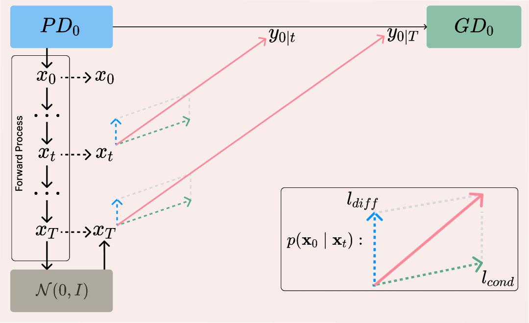
(a)

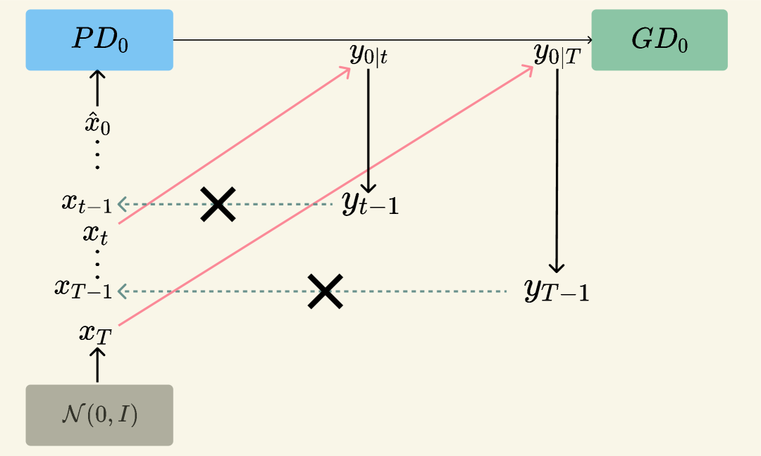
(b)

Figure 4: Explanation of Sampling Steps Disaster (SSD). With more than one target distributions, directly performing multiple steps inference yields error.

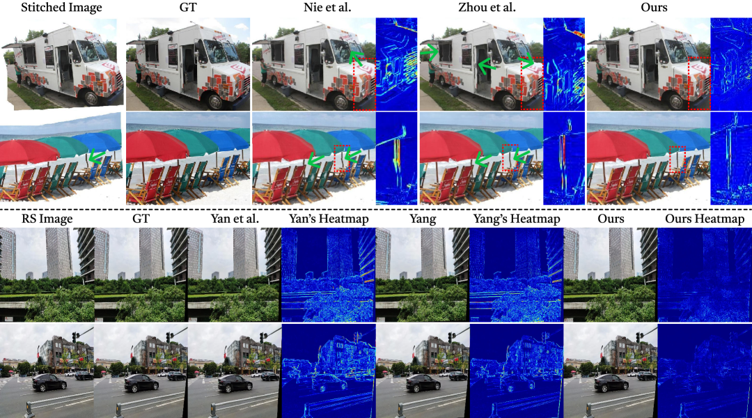
Figure 5: Comparing image rectangling (above the dotted line) and rolling shutter correction (below the dotted line) with previous methods. Green arrows points to artifacts or unsolved margins, and the red dashed boxes correspond to the area in the heatmap. The brighter areas on the heatmap indicate a greater discrepancy between the output and the ground truth.

3.3 Sampling Steps Disaster

In addition to the diffusion reconstruction loss, training diffusion models with additional losses, such as the condition and perceptual loss in our framework, has proved to be an effective way to enhance model performance [22, 52, 46]. However, after trained with additional losses, increasing sampling steps can lead to worse performance during inference, which is a seemingly counterintuitive phenomenon.

We take the condition loss as example to investigate this issue and illustrate our analysis in Fig. 4. We use the symbols $x_{t}$ and $z_{t}$ to represent elements from the Pseudo Label Distribution at timestep $t$ ($PD_{t}$) and the Ground Truth Distribution at the same timestep ($GD_{t}$), respectively. The loss functions $\ell_{diff}$ and $\ell_{cond}$ guide the model $\theta$ to learn the conditional distributions $p(x_{0}|x_{t})$ and $p(z_{0}|x_{t})$, shown by the blue and green dashed lines in Fig. 4(a). Under their joint constraint, the conditional distribution learned by our model $\theta$ is intermediate. We use the symbol $y_{0}$ to represent elements in the Learned Distribution ($LD_{t}$) between $PD_{t}$ and $GD_{t}$, with the conditional distribution $p(y_{0}|x_{t})$ indicated by the red arrow in Fig. 4(a).

Fig. 4(b) illustrates the inference process with multiple steps. In the first step, the model takes pure noise $x_{T}$ as input, generating an output $y_{0|T}$. The key issue arises in the second step. Instead of using $x_{T-1}$ as input, learned by the model during training, it uses $y_{T-1}$. Notably, $y_{T-1}$ has a different distribution with $x_{T-1}$. Thus, the inference chain is disrupted from the second step onward, as shown by the gray dashed arrow with a cross in Fig. 4(b). This error accumulates as sampling continues, as explained below:

Def.1. Use $\Delta_{t}$ to represent the difference between $x_{t}$ and $y_{t}$, that is, $\Delta_{t}\triangleq x_{t}-y_{t},t\in\{1,2,\dots,T\}$.

Def.2. Use $p$ to represent the composite mapping of the denoiser model $\theta:PD_{t}\to GD_{0},x_{t}\mapsto y_{0|t}$ and the forward process performed by the scheduler $s:GD_{0}\to GD_{t-1},y_{0|t}\mapsto y_{t-1}$, that is,

$$\begin{split}&p\triangleq s\circ\theta,\\ &p:PD_{t}\to GD_{t-1},x_{t}\mapsto y_{t-1}.\end{split}$$ (14)

In a multiple step inference, each sampling step performs a $p$ mapping on the results of the last step. Starting from $x_{T}$, inference is performed by:

$$\begin{split}pred_{1}&=p(\cdots p(p(x_{T}))\cdots).\end{split}$$ (15)

where $pred_{1}$ is the output with errors.

If we correct all the $y_{t}$ to $x_{t}$, as the dashed arrows in Fig. 4(b), the model could be able to inference properly, as $x_{t}$ is the condition that model $\theta$ learned in the training phase. The corrected output $pred_{2}$ is given by:

$$\begin{split}pred_{2}&=p(\cdots p(p(x_{T})+\Delta_{T-1})+\Delta_{T-2})\cdots).\end{split}$$ (16)

With the Euler method, the difference between $pred_{1}$ and $pred_{2}$ is given by:

$$\begin{split}error&=p(\cdots p(p(x_{T})+\Delta_{T-1})+\Delta_{T-2})\cdots)\\ &~~~~-p(\cdots p(p(x_{T}))\cdots)\\ &=\Delta_{0}+\Delta_{1}\bigtriangledown p(x_{1})+\Delta_{2}\bigtriangledown p(x_{2})\bigtriangledown p(x_{1})\\ &~~~~+\cdots+\Delta_{T-1}\Pi_{i=T-1}^{1}\bigtriangledown p(x_{i})\\ &=\Sigma_{i=0}^{T-1}\Delta_{i}\Pi_{j=i}^{1}\bigtriangledown p(x_{j}).\end{split}$$ (17)

When $T=1$ (one-step inference), the $error$ equals $0$. As the number of steps increases, the error rises exponentially. Results of different sampling steps are provided in Section 4.5. Detailed derivations are provided in Appendix. Sampling Steps Disaster

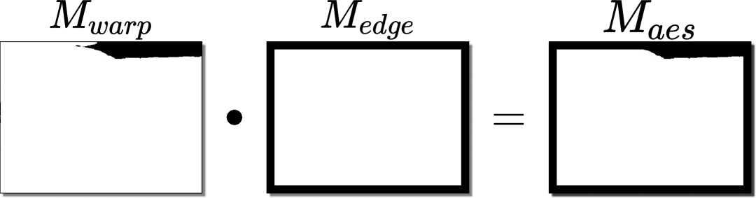
Figure 6: Calculation of $M_{aes}$.

3.4 Adaptive Ensemble Strategy

Diffusion models can produce inconsistent results with their generative nature. Besides, tasks like image rectangling involves warping images using a motion field, which makes addressing boundary issues challenging. Fortunately, both the problems can be effectively mitigated by aggregating different outputs together. If using a minimum filter, the pixels in white margins has the biggest values, so they will not be chosen during minimum-ensemble. However, applying such a filter can blur the edges, compromising image quality. To preserve edge details, we apply a median filter specifically to the non-boundary regions detected using warped mask $\mathcal{W}(M,\hat{F})$. As a result, our adaptive minimum-median filter allows us to ensemble the different outputs into a more uniform and higher-quality final image, which we call Adaptive Ensemble Strategy (AES).

Specifically, the mask for AES is the inner product of two masks, illustrated by Fig. 6. The first mask $M_{warp}$ is a mask varying from image to image, given by:

$$M_{warp}=\text{warp}(M,\hat{F}_{0|t}).$$ (18)

It is an adaptive mask revealing the remaining margins in a warped image. The Second mask $M_{edge}$ is a mask with fixed edges, ensuring the possible margins are not ignored because of the uncertainty of $M_{warp}$. Through the inner product operation, the final mask $M_{aes}$ marks the union of irregular margins from the two, given by:

$$M_{aes}=M_{warp}\cdot M_{edge}.$$ (19)

Pixels marked as margins in $M_{aes}$ will be applied with the minimum filter, others the median filter. Because RSC does not involve a mask, we only perform AES on the stitched image rectangling task.

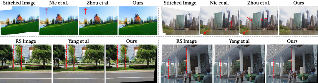
Figure 7: Generalization experiments. StableMotion excels in addressing irregular boundaries and resolving rolling shutter distortions.

 

Method	PSNR$\uparrow$	SSIM$\uparrow$	LPIPS$\downarrow$	FID$\downarrow$
He et al. [7]	14.70	0.378	-	38.19
Nie et al. [28]	21.28	0.714	0.152	21.77
CoupledTPS [29]	22.09	0.764	0.140	20.02
RecDiffusion [52]	22.21	0.773	0.789	18.75
StableMotion (Ours)	23.06	0.817	0.136	17.22

 

Table 1: Quantitative comparison of different methods on DIR-D testing set [28]. Best scores are highlighted in bold.

 

Method	PSNR$\uparrow$	SSIM$\uparrow$	LPIPS$\downarrow$	FID$\downarrow$
Yan et al. [45]	18.76	0.549	0.117	8.37
RS-Diffusion[46]	22.02	0.704	0.067	5.68
StableMotion (Ours)	22.65	0.724	0.068	5.18

 

Table 2: Quantitative comparison of different methods on RS-Real testing set [46]. Best scores are highlighted in bold.

4 Experiment

4.1 Implementation Details

StableMotion takes Stable Diffusion 2.0 as backbone and employ a 1000 time-step DDPM scheduler [10] for training. Learning rate was set at $2\times 10^{-5}$, with batch sizes of 128 for SIR and 32 for RSC. Training takes 60,000 steps, spanning 10 hours. For inference, it takes 32 ms to generate a rectified image on one NVIDIA H100. The weights of loss functions are set to be 1($\ell_{mse}$): 1($\ell_{cond}$): 0.01($\ell_{pct}$). The datasets are DIR-D [28] for SIR and RS-Real [46] for RSC.

4.2 Quantitative Comparison

We adopt two distortion metrics PSNR and SSIM, as well as two perceptual metrics LPIPS and FID for evaluation. For image rectangling, we include traditional method He et al. [7], the first deep-learning-based approach Nie et al. [28], the latest semi-supervised method CoupledTPS [29], and the latest diffusion model-based method RecDiffusion [52]. For rolling shutter correction, we include the homography mixture method [45] and the diffusion-based method [46]. As shown in Table. 1 and Table. 2, StableMotion achieves state-of-the-art performance in most categories. Specifically, StableMotion not only generate results closer to ground truths, improving metrics related to data consistency (PSNR and SSIM), but also delivers superior perceptual results with the semantic-aware priors from the pre-trained Stable Diffusion model (LPIPS and FID).

4.3 Qualitative Comparison

Our method is evaluated against the previous state-of-the-art methods on DIR-D [28] for SIR and on RS-Real [46] for RSC, as shown in Fig. 5. More visual results are provided in Appendix. Visual Comparison.

For SIR, we compare our results specifically with those of Nie et al. [28] and Zhou et al. [52]. Results of Nie et al. [28] are often misaligned, leaving visible local seams, as indicated by the green arrow in the figure. Zhou et al. [52] easily distorts both linear and non-linear structures, like the twisted car door in the first row. StableMotion excels in preserving both linear and non-linear features, minimizes the occurrence of white boundary artifacts, and fixes distortions in the input image. For RSC, StableMotion also produces results closer to ground truths, as reflected in significantly fewer bright spots in the align heatmap.

Further more, Previous stitching methods require warping operations to combine multiple images, which can easily cause distortions in the stitched results, as indicated by the green arrows in Fig. 5 (Stitched Image). Existing rectification methods have failed on these issues, resulting in preserved distortions. Fortunately, with content and structure priors from Stable Diffusion, StableMotion perceives semantic information and automatically corrects these local distortions caused by the original stitching process.

4.4 Generalizability Experiments

To test the generalization ability of out model, we perform zero-shot inference on APAP-Conssite dataset [48] with the model trained on DIR-D [28] for image rectangling (above the dotted line), and on newly captured RS images with the model trained on RS-Real [46] for rolling shutter correction (below the dotted line). As illustrated in Fig. 7, our model significantly outperforms the previous methods, particularly in handling white edges and linear structures and maintaining robustness across images from unseen distributions. We attribute this strong generalizability to the advantages of leveraging diffusion priors.

4.5 Sampling Steps Disaster

We test different numbers of inference steps with a DDIM scheduler [36]. Fig. 1 (the right part) provides the PSNR and SSIM of the results sampled from the same checkpoint with varying inference steps, and Fig. 8 provides visual results. As explained in Section 3.3, increasing sampling steps brings distortions into the predicted flows and results in a distorted warped image.

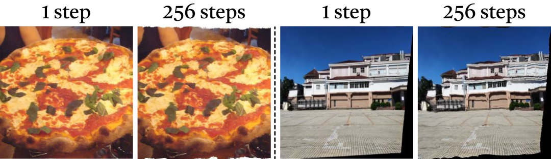
Figure 8: Visual comparison of different sampling steps with SSD.

4.6 Ablation Studies

Diffusion priors.

To demonstrate the importance of prior knowledge, we trained the same Stable Diffusion model on the same dataset [28] from scratch. All the hyperparameters remain the same. Without diffusion priors, the model failed to converge, and PSNR at different training steps is provided in Table 3. We believe that such a latent diffusion architecture with a VAE module requires enormous computing and multiple datasets to train from scratch, and a single task-specific dataset does not sufficiently support.

 

Priors	2k(steps)	4k	8k	16k	24k
✓	20.18	21.26	21.87	22.19	22.41
	11.06	11.88	12.00	11.95	11.93

 

Table 3: Ablation of diffusion priors, trained on DIR-D [28].

Training losses.

To demonstrate the effect of condition loss and perceptual loss, we trained two more models, one supervised exclusively by $\ell_{diff}$ and another by both $\ell_{diff}$ and $\ell_{cond}$. They are compared with the model trained using all three loss functions, and results are provided in Table. 4.

 

$\ell_{diff}$	$\ell_{cond}$	$\ell_{pl}$	PSNR$\uparrow$	SSIM$\uparrow$	TOPIQ$\uparrow$
✓			23.37	0.7957	0.7912
✓	✓		25.28	0.8351	0.8427
✓	✓	✓	25.50	0.8416	0.8511

 

Table 4: Ablaiton on loss items. Trained on RS-Real [46] dataset.

Adaptive ensemble strategy.

Impact of the number of ensemble is provided in Table 5, and visual results are shown in Fig. 9. AES has reduced the uncertainty nature of diffusion models, and addressed potentially unstable local areas as well as irregular boundaries in the image.

 

Ensemble num	1	2	4	8
PSNR	22.86	23.06	23.13	23.17

 

Table 5: Ablation of ensemble counts on image rectangling task.

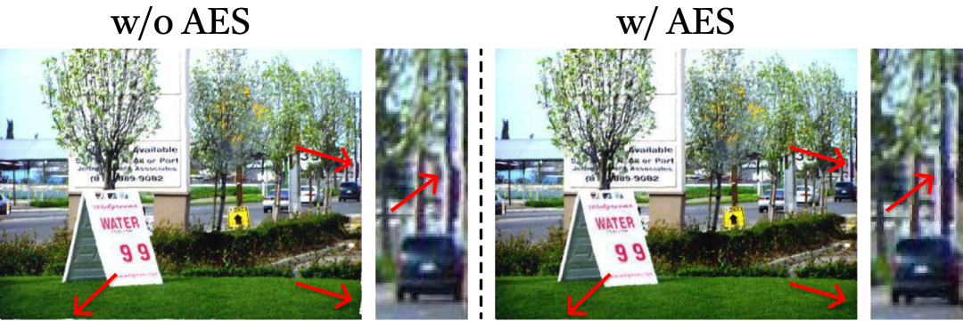
Figure 9: Distortions and boundaries are further repaired by AES.

Image-to-image framework

We tested image-to-image fine-tuning of SD on DIR-D [28], which converged to inferior results (PSNR=19.73). Visual resuts are provided in Fig. 10. With the generative nature of SD, the local details are unstable, which corrupts the model performance.

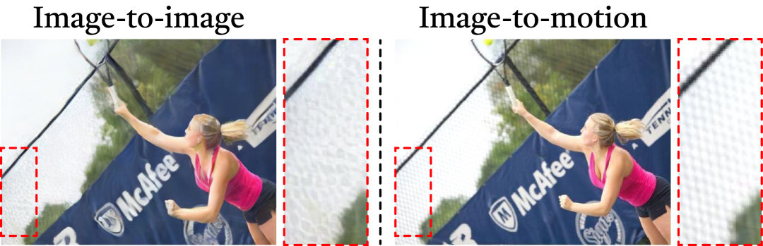
Figure 10: Compare StableMotion to image-to-image framework.

5 Conclusion

In this work, we present StableMotion, a framework to leverage image priors for motion estimation, and verify it on two tasks. Unlike previous image-prior based methods that took an image-to-image framework, or diffusion based methods that relied on high quality dataset and numerous computing to train from scratch, our method repurposes a text-to-image pre-trained model (Stable Diffusion) into an image-to-motion framework, performs one step inference, and achieves superior performance and generalizability. We also propose Sampling Steps Disaster (SSD), posing and explaining a hidden problem when a diffusion model has multiple learning objectives. SSD enables StableMotion to achieve one-step inference, and has the potential for broader applications in other diffusion-related tasks. We present Adaptive Ensemble Strategy (AES) to tackle the problem of diverse outputs from diffusion models. Overall, StableMotion sets a new standard in performance and generalizability, outperforming previous methods on public benchmarks.

Appendix

Sampling Steps Disaster

We propose Sampling Steps Disaster (SSD), which refers to the errors that occur when multi-step sampling is performed on the model that trained with multiple target distributions. Here we provide a more detailed derivation and give some intuitive explanation, and use the results of Zhou et al. [52] to support our theory.

Def.1. Use $\Delta_{t}$ to represent the difference between $x_{t}$ and $y_{t}$, that is, $\Delta_{t}\triangleq x_{t}-y_{t},t\in\{1,2,\dots,T\}$.

Def.2. Use $p$ to represent the composite mapping of the denoiser model $\theta:PD_{t}\to GD_{0},x_{t}\mapsto y_{0|t}$ and the forward process performed by the scheduler $s:GD_{0}\to GD_{t-1},y_{0|t}\mapsto y_{t-1}$, that is,

$$\begin{split}&p\triangleq s\circ\theta,\\ &p:PD_{t}\to GD_{t-1},x_{t}\mapsto y_{t-1}.\end{split}$$ (20)

In a multiple step inference, each sampling step performs a $p$ mapping on the results of the last step. Starting from $x_{T}$, inference is performed by:

$$\begin{split}pred_{1}&=p(\cdots p(p(x_{T}))\cdots).\end{split}$$ (21)

where $pred_{1}$ is the output with errors.

If correcting all the $y_{t}$ to $x_{t}$, the condition model learned in the training phase, the corrected process is given by:

$$\begin{split}&\hat{x}_{t}=\hat{y}_{t}+\Delta_{t},t\in\{0,1,\dots,T\},\\ &\hat{y}_{t-1}=p(\hat{x}_{t}),t\in{\{1,2,\dots,T\}},\\ \end{split}$$ (22)

where $\hat{x}_{0}$ is the output with the corrected condition at each timestep, represented by $pred_{2}$, that is:

$$pred_{2}=p(\cdots p(p(x_{T})+\Delta_{T-1})+\Delta_{T-2})\cdots).$$ (23)

Using the first-order Taylor expansion at point $x_{t}$ as well as the chain rule, we get:

$$\begin{split}pred_{2}&=p(\cdots p(p(x_{T})+\Delta_{T-1})+\Delta_{T-2})\cdots)\\ &=\Delta_{0}+\Delta_{1}\bigtriangledown p(x_{1})\\ &~~~~+p(\cdots p(p(x_{T})+\Delta_{T-1})+\Delta_{T-2})\cdots+\Delta_{2}))\\ &=\Delta_{0}+\Delta_{1}\bigtriangledown p(x_{1})+\Delta_{2}\bigtriangledown p(x_{1})\bigtriangledown p(x_{2})\\ &~~~~+p(\cdots p(p(x_{T})+\Delta_{T-1})+\Delta_{T-2})\cdots+\Delta_{3})))\\ &=\dots\\ &=\Delta_{0}+\Delta_{1}\bigtriangledown p(x_{1})+\Delta_{2}\Pi_{i=2}^{1}\bigtriangledown p(x_{i})\\ &~~~~+\cdots+\Delta_{T-1}\Pi_{i=T-1}^{1}\bigtriangledown p(x_{i})+p(\cdots p(p(x_{T}))\cdots)\\ &=\Sigma_{i=0}^{T-1}\Delta_{i}\Pi_{j=i}^{1}\bigtriangledown p(x_{j})+pred_{1}.\end{split}$$ (24)

The $error$ between $pred_{1}$ and $pred_{2}$ is given by:

$$\begin{split}error&=pred_{2}-pred_{1}\\ &=\Sigma_{i=0}^{T-1}\Delta_{i}\Pi_{j=i}^{1}\bigtriangledown p(x_{j})\end{split}$$ (25)

Such an error is intuitive. The denoiser have learned the conditional distribution of $p(y_{t-1}|x_{t})$, whose beginnings and endings does not match. As $t$ traverses, it fails to from an inference chain to $y_{0}$. Only performing one-step inference of $p(y_{0}|x_{T})$ makes sense.

For models with multiple training objectives, such as those have incorporated conditional losses, this phenomenon is commonly observed. Table. 6 shows the PSNR with different steps sampled from MDM [52] with a DDIM [36] scheduler, where the phenomenon of sampling steps disaster has also emerged.

 

Inference steps	1	4	16	64	256
PSNR	22.14	21.84	21.43	21.31	21.26

 

Table 6: SSD have also emerged in other works, such as MDM [52].

Visual Comparison

Below we provide more results on DIR-D [28] (image rectangling) and RS-Real [46] (rolling shutter correction), comparing with the results of Nie et al. [28], Zhou et al. [52], Yan et al. [45] and Yang et al. [46].

References

- Avidan and Shamir [2023] Shai Avidan and Ariel Shamir. Seam carving for content-aware image resizing. In Seminal Graphics Papers: Pushing the Boundaries, Volume 2, pages 609–617. 2023.
- Chen et al. [2024] Ziyang Chen, Daniel Geng, and Andrew Owens. Images that sound: Composing images and sounds on a single canvas. arXiv preprint arXiv:2405.12221, 2024.
- Dhariwal and Nichol [2021] Prafulla Dhariwal and Alexander Nichol. Diffusion models beat gans on image synthesis. In NeurIPS, pages 8780–8794, 2021.
- Fu et al. [2024] Xiao Fu, Wei Yin, Mu Hu, Kaixuan Wang, Yuexin Ma, Ping Tan, Shaojie Shen, Dahua Lin, and Xiaoxiao Long. Geowizard: Unleashing the diffusion priors for 3d geometry estimation from a single image. arXiv preprint arXiv:2403.12013, 2024.
- Geng et al. [2024a] Daniel Geng, Inbum Park, and Andrew Owens. Factorized diffusion: Perceptual illusions by noise decomposition. arXiv preprint arXiv:2404.11615, 2024a.
- Geng et al. [2024b] Daniel Geng, Inbum Park, and Andrew Owens. Visual anagrams: Generating multi-view optical illusions with diffusion models. In CVPR, pages 24154–24163, 2024b.
- He et al. [2013] Kaiming He, Huiwen Chang, and Jian Sun. Rectangling panoramic images via warping. ACM TOG, 32(4):1–10, 2013.
- Hedlin et al. [2024] Eric Hedlin, Gopal Sharma, Shweta Mahajan, Hossam Isack, Abhishek Kar, Andrea Tagliasacchi, and Kwang Moo Yi. Unsupervised semantic correspondence using stable diffusion. NeurIPS, 36:8266–8279, 2024.
- Ho and Salimans [2021] Jonathan Ho and Tim Salimans. Classifier-free diffusion guidance. In NeurIPS 2021 Workshop on Deep Generative Models and Downstream Applications, 2021.
- Ho et al. [2020] Jonathan Ho, Ajay Jain, and Pieter Abbeel. Denoising diffusion probabilistic models. In NeurIPS, pages 6840–6851, 2020.
- Hoogeboom et al. [2023] Emiel Hoogeboom, Jonathan Heek, and Tim Salimans. Simple diffusion: End-to-end diffusion for high resolution images. In ICML, pages 13213–13232, 2023.
- Hu et al. [2022] Edward J Hu, Yelong Shen, Phillip Wallis, Zeyuan Allen-Zhu, Yuanzhi Li, Shean Wang, Lu Wang, and Weizhu Chen. LoRA: Low-rank adaptation of large language models. In ICLR, 2022.
- Jiang et al. [2023] Hai Jiang, Ao Luo, Haoqiang Fan, Songchen Han, and Shuaicheng Liu. Low-light image enhancement with wavelet-based diffusion models. ACM TOG, 42(6), 2023.
- Jiang et al. [2024] Zhiying Jiang, Xingyuan Li, Jinyuan Liu, Xin Fan, and Risheng Liu. Towards robust image stitching: An adaptive resistance learning against compatible attacks. In AAAI, pages 2589–2597, 2024.
- Johnson et al. [2016] Justin Johnson, Alexandre Alahi, and Li Fei-Fei. Perceptual losses for real-time style transfer and super-resolution. In ECCV, pages 694–711. Springer, 2016.
- Karras et al. [2022] Tero Karras, Miika Aittala, Timo Aila, and Samuli Laine. Elucidating the design space of diffusion-based generative models. In NeurIPS, pages 26565–26577, 2022.
- Ke et al. [2024] Bingxin Ke, Anton Obukhov, Shengyu Huang, Nando Metzger, Rodrigo Caye Daudt, and Konrad Schindler. Repurposing diffusion-based image generators for monocular depth estimation. In CVPR, pages 9492–9502, 2024.
- Kingma and Welling [2014] Diederik P Kingma and Max Welling. Auto-encoding variational bayes. In ICLR, 2014.
- Lao and Ait-Aider [2018] Yizhen Lao and Omar Ait-Aider. A robust method for strong rolling shutter effects correction using lines with automatic feature selection. In ICCV, pages 4795–4803, 2018.
- Lee and Sim [2020] Kyu-Yul Lee and Jae-Young Sim. Warping residual based image stitching for large parallax. In CVPR, pages 8198–8206, 2020.
- Li et al. [2023] Alexander C Li, Mihir Prabhudesai, Shivam Duggal, Ellis Brown, and Deepak Pathak. Your diffusion model is secretly a zero-shot classifier. In ICCV, pages 2206–2217, 2023.
- Li et al. [2024] Haipeng Li, Hai Jiang, Ao Luo, Ping Tan, Haoqiang Fan, Bing Zeng, and Shuaicheng Liu. Dmhomo: Learning homography with diffusion models. ACM TOG, 2024.
- Liu et al. [2023] Xihui Liu, Dong Huk Park, Samaneh Azadi, Gong Zhang, Arman Chopikyan, Yuxiao Hu, Humphrey Shi, Anna Rohrbach, and Trevor Darrell. More control for free! image synthesis with semantic diffusion guidance. In WACV, pages 289–299, 2023.
- Lu et al. [2022] Cheng Lu, Yuhao Zhou, Fan Bao, Jianfei Chen, Chongxuan Li, and Jun Zhu. DPM-solver: A fast ode solver for diffusion probabilistic model sampling in around 10 steps. In NeurIPS, pages 5775–5787, 2022.
- Luo et al. [2024a] Grace Luo, Lisa Dunlap, Dong Huk Park, Aleksander Holynski, and Trevor Darrell. Diffusion hyperfeatures: Searching through time and space for semantic correspondence. NeurIPS, 36:47500–47510, 2024a.
- Luo et al. [2024b] Xiaotong Luo, Yuan Xie, Yanyun Qu, and Yun Fu. Skipdiff: Adaptive skip diffusion model for high-fidelity perceptual image super-resolution. In AAAI, pages 4017–4025, 2024b.
- Luo et al. [2024c] Ziwei Luo, Fredrik K Gustafsson, Zheng Zhao, Jens Sjölund, and Thomas B Schön. Taming diffusion models for image restoration: A review. arXiv preprint arXiv:2409.10353, 2024c.
- Nie et al. [2022] Lang Nie, Chunyu Lin, Kang Liao, Shuaicheng Liu, and Yao Zhao. Deep rectangling for image stitching: A learning baseline. In CVPR, pages 5740–5748, 2022.
- Nie et al. [2024] Lang Nie, Chunyu Lin, Kang Liao, Shuaicheng Liu, and Yao Zhao. Semi-supervised coupled thin-plate spline model for rotation correction and beyond. IEEE TPAMI, pages 1–13, 2024.
- Poole et al. [2023] Ben Poole, Ajay Jain, Jonathan T. Barron, and Ben Mildenhall. Dreamfusion: Text-to-3d using 2d diffusion. In ICLR, 2023.
- Rengarajan et al. [2016] Vijay Rengarajan, A. N. Rajagopalan, and R. Aravind. From bows to arrows: Rolling shutter rectification of urban scenes. In CVPR, pages 2773–2781, 2016.
- Rengarajan et al. [2017] Vijay Rengarajan, Yogesh Balaji, and A.N. Rajagopalan. Unrolling the shutter: Cnn to correct motion distortions. In CVPR, 2017.
- Rombach et al. [2022] Robin Rombach, Andreas Blattmann, Dominik Lorenz, Patrick Esser, and Björn Ommer. High-resolution image synthesis with latent diffusion models. In CVPR, pages 10684–10695, 2022.
- Saharia et al. [2022] Chitwan Saharia, William Chan, Saurabh Saxena, Lala Li, Jay Whang, Emily L Denton, Kamyar Ghasemipour, Raphael Gontijo Lopes, Burcu Karagol Ayan, Tim Salimans, et al. Photorealistic text-to-image diffusion models with deep language understanding. NeurIPS, 35:36479–36494, 2022.
- Sohl-Dickstein et al. [2015] Jascha Sohl-Dickstein, Eric Weiss, Niru Maheswaranathan, and Surya Ganguli. Deep unsupervised learning using nonequilibrium thermodynamics. In ICML, pages 2256–2265, 2015.
- Song et al. [2021a] Jiaming Song, Chenlin Meng, and Stefano Ermon. Denoising diffusion implicit models. In ICLR, 2021a.
- Song and Ermon [2019] Yang Song and Stefano Ermon. Generative modeling by estimating gradients of the data distribution. In NeurIPS, pages 1–9, 2019.
- Song et al. [2021b] Yang Song, Jascha Sohl-Dickstein, Diederik P Kingma, Abhishek Kumar, Stefano Ermon, and Ben Poole. Score-based generative modeling through stochastic differential equations. In ICLR, 2021b.
- Szeliski et al. [2007] Richard Szeliski et al. Image alignment and stitching: A tutorial. Foundations and Trends® in Computer Graphics and Vision, 2(1):1–104, 2007.
- Tang et al. [2023] Luming Tang, Menglin Jia, Qianqian Wang, Cheng Perng Phoo, and Bharath Hariharan. Emergent correspondence from image diffusion. In NeurIPS, pages 1363–1389, 2023.
- Wang et al. [2023a] Jinglong Wang, Xiawei Li, Jing Zhang, Qingyuan Xu, Qin Zhou, Qian Yu, Lu Sheng, and Dong Xu. Diffusion model is secretly a training-free open vocabulary semantic segmenter. arXiv preprint arXiv:2309.02773, 2023a.
- Wang et al. [2023b] Yinhuai Wang, Jiwen Yu, and Jian Zhang. Zero-shot image restoration using denoising diffusion null-space model. In ICLR, 2023b.
- Wu et al. [2024] Rundi Wu, Ben Mildenhall, Philipp Henzler, Keunhong Park, Ruiqi Gao, Daniel Watson, Pratul P Srinivasan, Dor Verbin, Jonathan T Barron, Ben Poole, et al. ReconFusion: 3d reconstruction with diffusion priors. In CVPR, pages 21551–21561, 2024.
- Xiao et al. [2023] Changming Xiao, Qi Yang, Feng Zhou, and Changshui Zhang. From text to mask: Localizing entities using the attention of text-to-image diffusion models. arXiv preprint arXiv:2309.04109, 2023.
- Yan et al. [2023] Weilong Yan, Robby T. Tan, Bing Zeng, and Shuaicheng Liu. Deep homography mixture for single image rolling shutter correction. In ICCV, pages 9868–9877, 2023.
- Yang et al. [2024] Zhanglei Yang, Haipeng Li, Mingbo Hong, Bing Zeng, and Shuaicheng Liu. Single image rolling shutter removal with diffusion models. arXiv preprint arXiv:2407.02906, 2024.
- Yuan and Yuan [2024] Yutao Yuan and Chun Yuan. Efficient conditional diffusion model with probability flow sampling for image super-resolution. In AAAI, pages 6862–6870, 2024.
- Zaragoza et al. [2013] Julio Zaragoza, Tat-Jun Chin, Michael S Brown, and David Suter. As-projective-as-possible image stitching with moving dlt. In CVPR, pages 2339–2346, 2013.
- Zhang et al. [2024a] Junyi Zhang, Charles Herrmann, Junhwa Hur, Luisa Polania Cabrera, Varun Jampani, Deqing Sun, and Ming-Hsuan Yang. A tale of two features: Stable diffusion complements dino for zero-shot semantic correspondence. NeurIPS, 36:45533–45547, 2024a.
- Zhang et al. [2023] Lvmin Zhang, Anyi Rao, and Maneesh Agrawala. Adding conditional control to text-to-image diffusion models. In ICCV, pages 3836–3847, 2023.
- Zhang et al. [2024b] Yun Zhang, Yukun Lai, Nie Lang, Fang-Lue Zhang, and Lin Xu. Recstitchnet: Learning to stitch images with rectangular boundaries. Computational Visual Media, 2024b.
- Zhou et al. [2023] Tianhao Zhou, Haipeng Li, Ziyi Wang, Ao Luo, ChenLin Zhang, Jiajun Li, Bing Zeng, and Shuaicheng Liu. Recdiffusion: Rectangling for image stitching with diffusion models. In CVPR, pages 1–10, 2023.
- Zhu et al. [2022] Fushun Zhu, Shan Zhao, Peng Wang, Hao Wang, Hua Yan, and Shuaicheng Liu. Semi-supervised wide-angle portraits correction by multi-scale transformer. In CVPR, pages 19689–19698, 2022.
- Zhuang et al. [2019] Bingbing Zhuang, Quoc-Huy Tran, Pan Ji, Loong-Fah Cheong, and Manmohan Chandraker. Learning structure-and-motion-aware rolling shutter correction. In CVPR, 2019.