A $G_{2}$-Holonomy Model for Late-Time Cosmic Acceleration in M-theory: Alleviating the Hubble Tension through Geometric Vacuum Energy

Abstract

A framework is developed within an eleven-dimensional M-theory scenario where dynamical geometric moduli, originating from a $G_{\mathrm{2}}$-holonomy compactification, generate an evolving cosmological term, $\Lambda(z)$. This “geometric vacuum energy” is primarily attributed to extra-dimensional fluxes and instanton-like corrections embedded within the moduli potential. Crucially, evolving the model from early cosmic times reveals strong attractor behaviors. With an appropriate choice for the moduli potential parameters (specifically, the location of the Gaussian feature, $\phi_{c}\approx 5.0$, and a fine-tuned overall potential scale $V_{0}$), a natural attractor solution emerges that alleviates the Hubble tension. This solution yields an inferred $H_{0}\approx 69.4\ \mathrm{km}\,\mathrm{s}^{-1}\,\mathrm{Mpc}^{-1}$ (evolving from $H_{0}\approx 67\ \mathrm{km}\,\mathrm{s}^{-1}\,\mathrm{Mpc}^{-1}$ typically favored by early-Universe probes in simpler models) and a present-day cosmological term $\Lambda(0)\approx 1.105\times 10^{-52}\ \mathrm{m}^{-2}$, consistent with observational constraints, all while maintaining $\Phi(0)\approx 2.2$. This occurs without significantly disturbing the overall concordance, accommodating mild spatial openness ($\Omega_{k0}\approx 0.097$), a slightly reduced matter fraction ($\Omega_{m0}\approx 0.25$), and a cosmic age near $13.8\mathrm{Gyr}$. This attractor solution is fully consistent with early Universe constraints (BBN and CMB), where the geometric vacuum energy remains subdominant. Quantitative assessment against 34 cosmic chronometer $H(z)$ data points demonstrates excellent fit ($\chi^{2}/N\approx 0.44$). The model also yields $S_{8}\approx 0.74$. These findings highlight a pathway where a $G_{\mathrm{2}}$-compactified M-theory framework can naturally reconcile late-time cosmological observations through attractor dynamics of its geometric moduli, suggesting a UV-complete origin for a dynamical vacuum energy. Further investigations into the parameter space and observational signatures are envisaged.

I Introduction

An alternative avenue involves replacing the strictly constant $\Lambda$ with a dynamically evolving term…

An alternative avenue involves replacing the strictly constant $\Lambda$ with a dynamically evolving term, $\Lambda(z)$, particularly one rooted in fundamental theory. Specific M-theory compactifications on manifolds with $G_{2}$-holonomy offer such a possibility [1, 2]. In these scenarios, geometric moduli fields associated with the extra dimensions can remain light and evolve slowly over cosmic time. Their potential energy, from fluxes and non-perturbative effects like instantons, can contribute an effective vacuum energy $\Lambda(z)$ that mimics a constant at late times (low $z$) but deviates at earlier epochs [3, 4].

The present work investigates the cosmological viability of such a geometry-driven $\Lambda(z)$ model derived from $G_{2}$-holonomy M-theory. A concrete model featuring exponential and Gaussian terms in the moduli potential—motivated by flux and instanton contributions—is constructed. Initially, analysis of the late-time Universe demonstrated the model’s capacity to accommodate an $H_{0}\approx 69.5\ \mathrm{km}\,\mathrm{s}^{-1}\,\mathrm{Mpc}^{-1}$, thereby partially alleviating the Hubble tension, while maintaining consistency with other constraints like the cosmic age. Crucially, this study extends the investigation to the early Universe dynamics, exploring the evolution of the moduli fields from early cosmological epochs towards the present. We demonstrate that for specific, physically motivated choices of the potential parameters (notably, the position of the Gaussian feature, $\phi_{c}\approx 5.0$, and a corresponding fine-tuning of the overall potential scale $V_{0}$), the model exhibits robust attractor solutions. These attractors naturally lead to a present-day state characterized by $w_{0}\approx-1.0000$, a Hubble constant $H_{0}\approx 69.4\ \mathrm{km}\,\mathrm{s}^{-1}\,\mathrm{Mpc}^{-1}$, and a cosmological term $\Lambda(0)\approx 1.105\times 10^{-52}\ \mathrm{m}^{-2}$, all while being consistent with early Universe (BBN, CMB) constraints and keeping the scalar field excursions within more controlled limits. This finding suggests that the alleviation of the Hubble tension can be a natural consequence of the model’s attractor dynamics, rather than requiring fine-tuned late-time conditions. By grounding $\Lambda(z)$ in the geometry of M-theory, this approach also offers a potential pathway toward addressing fine-tuning problems associated with the cosmological constant from a UV-complete perspective.

In this investigation, the detailed theoretical framework is presented, and the effective cosmological dynamics, including early-Universe evolution and attractor behaviors, are derived. The model, particularly its promising attractor solutions, is confronted with current observational data. While related $G_{2}$ compactifications may also be relevant for alternative cosmological histories, such as cyclic or ekpyrotic models [5, 6], the primary focus here is on the potential of this mechanism within the standard expanding Universe paradigm to naturally resolve late-time tensions through its intrinsic dynamics.

The paper is structured as follows: Section II reviews the theoretical background of M-theory compactifications on $G_{2}$ manifolds and the origin of moduli fields, including the formulation of the scalar potential and the equations of motion. Section III details the observational data context and the numerical methods employed to solve the model’s dynamical equations and identify attractor solutions. Section IV presents the main results, commencing with a summary of initial late-time phenomenological explorations, followed by a detailed investigation of early-Universe attractor solutions and the identification of an optimal scenario that alleviates the Hubble tension, including its goodness-of-fit to Cosmic Chronometer data. Section V discusses the implications of these findings, focusing on cosmological tensions, model features, the significance of the attractor dynamics, and model limitations. Finally, Section VI summarizes the findings and outlines future directions. Appendices provide further details on specific calculations and parameter sets.

II Theoretical Background

This section outlines the model’s theoretical underpinnings, starting from the M-theory framework and $G_{2}$-holonomy compactification. This leads to an effective four-dimensional description featuring dynamical moduli fields and their associated potential.

II.1 Moduli from $G_{2}$-Holonomy Manifolds

M-theory, formulated in eleven spacetime dimensions, provides a rich framework for unification. Compactification of M-theory on a seven-dimensional manifold $X_{7}$ endowed with special $G_{2}$-holonomy is a well-established route to obtaining effective four-dimensional theories with $\mathcal{N}=1$ supersymmetry [1, 2]. Such compactifications naturally give rise to numerous scalar fields in the 4D effective theory, known as moduli, which parameterize the size and shape of the internal manifold $X_{7}$ and the configuration of fields residing within it.

Most of these moduli typically arise from the dimensional reduction of the 11D three-form gauge field $C_{3}$. Their vacuum expectation values correspond to geometric properties, such as the volumes of topologically non-trivial three-cycles and four-cycles within $X_{7}$. While many of these moduli are expected to acquire large masses and become stabilized (fixed) at high energy scales through mechanisms involving background fluxes or nonperturbative quantum effects, it is plausible that a subset remains relatively light even at low energies. These light moduli can then play a significant role in late-time cosmology. For phenomenological exploration, it is often assumed, as in the present framework, that the dynamics are dominated by a small number of such light fields; here, attention is focused on two representative light moduli, denoted $\phi_{1}$ and $\phi_{2}$, treating the others as stabilized.

II.2 Moduli Potential and Emergent $\Lambda(z)$

A scalar potential governs the dynamics of the light moduli $\phi_{i}$ in the effective 4D theory, $V(\phi_{1},\phi_{2},\ldots)$. The specific details of the manifold $X_{7}$, the choice of background fluxes threading its cycles, and nonperturbative contributions, such as those from M-brane instantons wrapping internal cycles, determine the precise form of this potential.

In many explicit $G_{2}$-holonomy constructions, the resulting potential $V$ exhibits characteristic features. It often includes terms with exponential dependence on the moduli fields, typically arising from flux contributions or M5-brane instanton effects. Furthermore, localized contributions, sometimes approximated as Gaussian-like terms, can appear, potentially linked to specific geometric transitions or localized sources in the internal manifold. A schematic form encapsulating these standard features for a combined light field $\Phi\equiv\phi_{1}+\phi_{2}$ can be written as:

$$V(\Phi) =V_{0}\,\biggl{[}1+\epsilon_{1}\,e^{-\alpha_{1}\,\Phi}+\epsilon_{2}\,e^{-\alpha_{2}\,\Phi}$$

$$\quad+\epsilon_{3}\,\exp\!\bigl{\{}-\lambda\,(\Phi-\phi_{c})^{2}\bigr{\}}\biggr{]}.$$ (1)

Here, $V_{0}$ sets the overall scale, while the parameters $\{\epsilon_{i},\alpha_{i},\lambda,\phi_{c}\}$ are determined by the compactification details (see Sec. VI). This potential forms the basis for the dynamical vacuum energy in the model.

This potential energy (Eq. (1)) acts as a source for a dynamical vacuum energy density, $\rho_{\Lambda}(z)=V[\Phi(z)]$, contributing to the cosmic expansion via an effective, time-varying cosmological term:

$$\Lambda(z)=8\pi GV[\Phi(z)].$$ (2)

Here, $G$ is Newton’s gravitational constant.

II.3 Geometric Origins of the Potential Structure

The specific structure of the potential in Eq. (1), particularly the exponential and Gaussian-like terms, is not arbitrary but is motivated by the underlying geometry and physics of M-theory compactifications. Key elements include:

• Manifold Construction and Topology: $G_{2}$-holonomy manifolds can be constructed using various techniques, such as resolving orbifolds (Joyce manifolds [7, 8]) or employing twisted connected sum (TCS) methods [9, 10]. The topology of the resulting manifold $X_{7}$, particularly its Betti numbers (e.g., $b_{3}$, counting three-cycles), determines the number and type of massless moduli fields before stabilization.

• Fluxes and Instantons: Background fluxes of the M-theory four-form field $G_{4}$ threading cycles in $X_{7}$ are crucial for stabilizing many moduli. These fluxes are quantized, leading to discrete choices. Both flux contributions and nonperturbative effects from M5-branes wrapping six-cycles (M5-instantons) can generate exponential terms $e^{-a_{i}\Phi}$ in the 4D effective potential $V(\Phi)$. Furthermore, specific geometric features or transitions, such as partial conifold transitions, might be associated with localized effects in the potential, potentially giving rise to the Gaussian-like terms.

• Moduli Stabilization: While the topology might allow for many potential moduli, the interplay of fluxes and nonperturbative effects typically fixes most of them at specific values (stabilization), giving them large masses. In this case, the remaining light fields, $\phi_{1},\phi_{2}$, represent the residual flat directions or pseudo-moduli whose dynamics govern the low-energy phenomenology.

Therefore, the parameters $\{\epsilon_{i},\alpha_{i},\lambda,\phi_{c}\}$ appearing in the schematic potential are, in principle, determined by these discrete flux choices and the topological data of the $G_{2}$ manifold, rather than being arbitrary ad hoc parameters. This provides a potential path towards a geometric and UV-complete origin for dynamical dark energy $\Lambda(z)$.

The interplay between these different contributions (e.g., the exponentially decaying terms and the localized Gaussian feature) leads to a non-trivial potential landscape, the specific features of which are sensitive to parameters like $\phi_{c}$. As will be demonstrated in Sec. IV, this sensitivity allows for the emergence of different attractor solutions when the system evolves from the early Universe. For certain parameter regimes relevant to late-time cosmology, the scalar field $\Phi(z)$ can evolve in regions where the slope of the potential $V^{\prime}(\Phi)=dV/d\Phi$ is negative. This feature, which can contribute to an effective equation of state $w(z)<-1$ under specific approximations like a late-time ansatz (as explored in earlier analyses and detailed for the original benchmark in Appendix A), is put into a broader context by the full early-to-late Universe evolution. This complete evolution, discussed in detail in Sec. IV and Sec. V, reveals a richer dynamical structure leading to specific present-day values for $w_{0}$ and $H_{0}$, including the optimal attractor solution that alleviates the Hubble tension.

II.4 Slow-Roll Approximation

The cosmological evolution of the light moduli fields $\phi_{i}$ (or the combined field $\Phi$) is governed by their equation of motion derived from the effective action, coupled to the background expansion. In many scenarios involving scalar fields with relatively flat potentials, the fields can enter a dynamical regime known as slow-roll, where their kinetic energy is subdominant compared to their potential energy:

$$\frac{1}{2}\dot{\Phi}^{2}\ll|V(\Phi)|.$$ (3)

When this condition holds, the field’s evolution is slow and can often be approximated by a simple functional form. A common outcome, particularly for potentials with exponential terms or in attractor regimes [3], is a near-logarithmic evolution with redshift:

$$\Phi(z)\approx\Phi_{0}+\kappa\,\ln(1+z).$$ (4)

This ansatz, where $\Phi_{0}$ is a present-day reference value and $\kappa$ parameterizes a hypothetical late-time evolution rate, implies that if the field were to follow such a trajectory, it would evolve very slowly at late times, allowing the resulting geometric vacuum energy $\Lambda(z)=8\pi GV[\Phi(z)]$ to mimic a cosmological constant today while deviating at earlier epochs. This logarithmic form (Eq. (4)) has been a common approximation for certain scalar field dynamics and served as an initial phenomenological guide in previous stages of this work, particularly for late-time analyses (as detailed in Appendix C for calculating $w(z)$ under this ansatz). However, the present study focuses on the full numerical solutions of the equation of motion (Sec. II.5) evolving from the early Universe. These solutions reveal richer attractor dynamics that determine the actual present-day values of $\Phi(0)$ and its evolution, which may or may not precisely follow this simple logarithmic form, especially concerning the specific values of $\Phi_{0}$ and $\kappa$ that best describe the late-time attractor behavior. The validity of any slow-roll conditions will be assessed a posteriori from these full numerical solutions.

II.5 Equation of Motion

While the logarithmic ansatz (Eq. (4)) is used for the primary analysis, the fundamental dynamics of the scalar field $\Phi$ are derived from an effective action. Assuming a canonical kinetic term for $\Phi$ minimally coupled to gravity, the Lagrangian is:

$$\mathcal{L}_{\Phi}=\frac{1}{2}(\partial_{\mu}\Phi)(\partial^{\mu}\Phi)-V(\Phi).$$ (5)

(Potential non-canonical terms are assumed negligible or absorbed into definitions.) Varying the action yields the equation of motion in a spatially flat FLRW background:

$$\ddot{\Phi}+3H(t)\dot{\Phi}+\frac{dV}{d\Phi}=0,$$ (6)

$$w_{\phi}(z)=\frac{\frac{1}{2}\dot{\Phi}^{2}-V(\Phi)}{\frac{1}{2}\dot{\Phi}^{2}+V(\Phi)}$$ (7)

where dots denote derivatives concerning cosmic time $t$, and $H(t)=\dot{a}/a$ is the Hubble parameter. This equation governs the exact evolution $\Phi$, and its numerical solution can be used to verify the validity of the slow-roll approximation and the logarithmic ansatz for specific parameter sets.

Here, $H(z)$ is the Hubble parameter at redshift $z$, $H_{0}=H(z=0)$ is the Hubble constant, and $\Omega_{i0}$ represents the density parameters today. These parameters adhere to the sum rule:

$$\Omega_{m0}+\Omega_{r0}+\Omega_{k0}+\Omega_{\mathrm{geom0}}=1,$$ (8)

where $\Omega_{\mathrm{geom0}}$ is the present-day density parameter for the geometric vacuum energy, defined as:

$$\Omega_{\mathrm{geom0}}=\Omega_{\mathrm{geom}}(z=0)=\frac{\Lambda(0)}{3H_{0}^{2}}.$$ (9)

$$\Lambda(z)=8\pi GV[\Phi(z)]$$ (10)

The term $\Lambda(0)$ is evaluated using $V[\Phi(z=0)]$, where $\Phi(z=0)$ is the present-day value of the scalar field obtained from the full numerical solution of its equation of motion. The dynamical component $\Omega_{\mathrm{geom}}(z)=\Lambda(z)/(3H_{0}^{2})$ is then explicitly calculated using $V[\Phi(z)]$ (Eq. (1)) and $\Lambda(z)$ (Eq. (10)), where $\Phi(z)$ is determined by numerically solving Eq. (6) coupled to the Friedmann equation. The standard Friedmann equation governing the expansion history $H(z)$ is given by:

$$\frac{H(z)^{2}}{H_{0}^{2}}=\Omega_{m0}(1+z)^{3}+\Omega_{r0}(1+z)^{4}+\Omega_{k0}(1+z)^{2}+\Omega_{\mathrm{geom0}}\frac{\Lambda(z)}{\Lambda(0)}.$$ (11)

This equation, with $\Lambda(z)$ determined by the evolving scalar field $\Phi(z)$ from the numerical solution, is the primary input for comparing the model against observational data and for studying its early Universe dynamics and attractor solutions.

III Data and Statistical Methodology

This section details the observational datasets used for context and comparison, and the numerical methods employed to solve the model’s dynamical equations and assess the properties of its attractor solutions.

III.1 Observational Data Context

The viability of the cosmological scenarios emerging from our model, particularly concerning late-time observables like $H_{0}$ and the expansion history, is assessed in the context of several standard cosmological probes. These provide benchmarks and highlight existing tensions the model aims to address. The primary datasets considered for this contextual comparison include:

• Cosmic Microwave Background (CMB): Results from the Planck satellite (e.g., [11]) provide crucial constraints on early-Universe parameters and the inferred $H_{0}$ within the standard $\Lambda$CDM model, forming a key part of the Hubble tension.

• Baryon Acoustic Oscillations (BAO): Measurements of the BAO scale from galaxy surveys (e.g., 6dFGS [12], SDSS MGS [13], BOSS DR12 [14]) constrain $H(z)$ and the angular diameter distance $D_{A}(z)$, providing standard rulers for the expansion history.

• Type Ia Supernovae (SNe): Luminosity distance measurements from compilations like Pantheon [15] probe the expansion history at lower redshifts ($z\lesssim 2$) and were instrumental in discovering cosmic acceleration.

• Hubble Constant ($H_{0}$): Direct local measurements of $H_{0}$ (e.g., from SH0ES [16]) yield higher values than those inferred from CMB data within $\Lambda$CDM, defining the Hubble tension. Our model’s ability to produce an $H_{0,\mathrm{evolved}}$ closer to these local measurements is a key point of investigation.

• Growth of Structure ($S_{8}$): Constraints from weak lensing surveys (e.g., DES [17], KiDS [18]) test the model’s predictions for structure formation.

• Cosmic Chronometers (CC): Direct measurements of $H(z)$ from the differential age evolution of passive galaxies (e.g., as compiled in [19]) provide valuable data points for the expansion history, against which specific model solutions (like the attractor solutions found) can be tested for goodness-of-fit.

The precise likelihood implementations for these datasets are standard in the literature and are invoked when discussing the consistency of our model’s predictions with established constraints.

III.2 Numerical and Analytical Methods

The core of this work involves numerically solving the coupled system of the Friedmann equation (Eq. (11)) and the scalar field equation of motion (Eq. (6)) from early cosmic times ($N_{\mathrm{start}}\ll 0$) to the present day ($N=0$). This allows for the exploration of the model’s dynamical trajectories and the identification of attractor solutions.

The following approaches are employed:

• Numerical Integration: The system of ordinary differential equations is solved using a standard Runge-Kutta method (specifically, scipy.integrate.solve_ivp in Python implementations) with appropriate precision controls. This yields the evolution of $\Phi(N)$ and $\Psi(N)=d\Phi/dN$.

• Parameter Space Exploration: To understand the model’s behavior, particularly the impact of the potential parameter $\phi_{c}$ on late-time cosmology, we explore a grid of initial conditions for $\Phi(N_{\mathrm{start}})$ and $\Psi(N_{\mathrm{start}})$ for different choices of $\phi_{c}$. The resulting present-day values ($\Phi(0)$, $\Psi(0)$, $w_{0}$, and the emergent $H_{0,\mathrm{evolved}}$) are analyzed to identify attractor behaviors.

• Consistency Checks: For each evolved solution, consistency with early Universe constraints (e.g., ensuring $\Omega_{\mathrm{geom}}(z)$ is subdominant during BBN and CMB epochs) is verified. The present-day equation of state $w_{0}$ and the emergent $H_{0,\mathrm{evolved}}$ (derived from $E^{2}(z=0)$ relative to the input $H_{0,\mathrm{fiducial}}$ used for normalization) are key outputs.

• Goodness-of-Fit (for specific solutions): For promising attractor solutions that yield specific cosmological parameters (e.g., $H_{0}\approx 69.4\ \mathrm{km}\,\mathrm{s}^{-1}\,\mathrm{Mpc}^{-1}$), their fit to relevant datasets, such as the cosmic chronometer $H(z)$ data, is assessed using the chi-squared statistic ($\chi^{2}/N$).

• Model Comparison Context (AIC/BIC): When comparing the overall performance of a specific realization of our model (e.g., the attractor solution with $\phi_{c}\approx 5.0$) against $\Lambda$CDM using metrics like $\chi^{2}_{\mathrm{min}}$ from specific datasets, standard model selection criteria like the Akaike Information Criterion (AIC) [20] and Bayesian Information Criterion (BIC) [21] can provide context on model preference, accounting for differences in parameter numbers ($k$).

The cosmic age $t_{0}$ for any given successful cosmological evolution is calculated numerically by integrating $1/((1+z)H(z))$, as detailed in Appendix E.

IV Results

This section presents the main cosmological results derived from the $G_{2}$-holonomy model for geometric vacuum energy. We begin by summarizing the initial phenomenological insights gained from a late-time ansatz for the scalar field evolution. Subsequently, we detail the core findings of this work: the numerical evolution of the model from early cosmic times, the identification of its attractor solutions, and the crucial role of the potential parameter $\phi_{c}$ in achieving a late-time cosmology that can alleviate the Hubble tension while remaining consistent with other observational constraints.

IV.1 Initial Late-Time Phenomenological Exploration: A Summary

Prior phenomenological investigations of the model, utilizing a simplified late-time logarithmic ansatz for the scalar field evolution, $\Phi(z)\approx\Phi_{0}+\kappa\ln(1+z)$ (Eq. (4)), suggested that the model possessed the flexibility to address the Hubble tension. Specifically, with a benchmark set of potential parameters where the Gaussian peak was centered at $\phi_{c}=7.6$ (detailed in Appendix A), it was found that choices such as $\Phi_{0}\approx 2.0$ and $\kappa\approx 0.7$, when combined with mild spatial openness ($\Omega_{k0}\approx 0.097$) and a slightly reduced matter fraction ($\Omega_{m0}\approx 0.25$), could yield an inferred $H_{0}\approx 69.5\,\mathrm{km\,s}^{-1}\,\mathrm{Mpc}^{-1}$. Constraints derived from MCMC analyses based on this late-time ansatz and combined datasets (such as CMB+BAO+SNe) were explored in earlier iterations of this work, demonstrating the model’s initial potential.

While these initial explorations were promising, they relied on a specific ansatz for the late-time behavior of $\Phi(z)$. A more fundamental understanding requires numerically solving the full dynamical equations from the early Universe to determine the natural evolutionary paths and present-day observables of the model. This comprehensive approach is presented next and forms the primary results of this paper.

IV.2 Early Universe Evolution and Emergence of Attractor Solutions

To determine the natural cosmological evolution predicted by the $G_{2}$-holonomy model, we numerically integrate the coupled system comprising the Friedmann equation (Eq. (11)) and the scalar field equation of motion (Eq. (6)). The evolution is initiated at an early epoch, typically $N_{\mathrm{start}}=-15$ (corresponding to redshift $z\approx 3.27\times 10^{6}$), and proceeds to the present day ($N=0$). This methodology allows us to explore the existence of attractor solutions, which are late-time behaviors that are largely insensitive to a wide range of initial conditions for the scalar field $\Phi(N_{\mathrm{start}})$ and its derivative $\Psi(N_{\mathrm{start}})=d\Phi/dN|_{N_{\mathrm{start}}}$.

We investigate the impact of varying the Gaussian peak parameter, $\phi_{c}$, in the potential (Eq. (1)), while keeping other potential shape parameters ($\epsilon_{1}=0.60,\alpha_{1}=1.5,\epsilon_{2}=0.47,\alpha_{2}=0.7,\epsilon_{3}=0.60,\lambda_{g}=0.28$) fixed to their original benchmark values (see Appendix A). The overall potential scale $V_{0}$ is a crucial parameter. For the primary results presented below, $V_{0}$ is fine-tuned to $V_{0}=4.9775\times 10^{-27}\,\mathrm{kg\,m}^{-3}$ when $\phi_{c}=5.0$. This specific tuning ensures that the corresponding attractor solution (which yields $\Phi(0)\approx 2.20$) results in a present-day cosmological term $\Lambda(0)\approx 1.105\times 10^{-52}\,\mathrm{m}^{-2}$ and an evolved Hubble constant $H_{0,\mathrm{evolved}}\approx 69.42\,\mathrm{km\,s}^{-1}\,\mathrm{Mpc}^{-1}$ (i.e., $E^{2}(0)\approx 1$ for an input $H_{0,\mathrm{fiducial}}=69.5\,\mathrm{km\,s}^{-1}\,\mathrm{Mpc}^{-1}$). For other trial values of $\phi_{c}$ shown for comparison in Table 1, the reference $V(\Phi=2.0,\phi_{c})$ used for normalizing $\Omega_{\mathrm{geom0\_target}}$ is re-evaluated with the respective $\phi_{c}$ but using this same fine-tuned $V_{0}=4.9775\times 10^{-27}\,\mathrm{kg\,m}^{-3}$.

The key findings from this exploration are summarized in Table 1. All reported attractor solutions robustly satisfy early Universe constraints, with $\Omega_{\mathrm{geom}}(z)$ being dynamically suppressed to negligible levels during the epochs of Big Bang Nucleosynthesis (BBN) and CMB formation (e.g., $\Omega_{\mathrm{geom}}(z\sim 1100)\sim 10^{-9}$).

Table 1: Summary of attractor solutions at $z=0$ for different trial values of the Gaussian peak parameter $\phi_{c}$ in the potential $V(\Phi)$ (Eq. (1)). The table displays the present-day scalar field value $\Phi(0)$, its derivative with respect to e-folds $\Psi(0)=d\Phi/dN|_{N=0}$, the equation of state parameter $w_{0}$, the squared Hubble normalization factor $E^{2}(0)=(H_{0,\mathrm{evolved}}/H_{0,\mathrm{input}})^{2}$ (where $H_{0,\mathrm{input}}=69.5\,\mathrm{km\,s}^{-1}\mathrm{Mpc}^{-1}$), the resulting evolved Hubble constant $H_{0,\mathrm{evolved}}$, and the calculated present-day cosmological term $\Lambda(0)$ in $10^{-52}\,\mathrm{m}^{-2}$. These attractors are reached from a broad range of initial conditions. Other potential parameters are fixed as per Appendix A, and $V_{0}=4.9775\times 10^{-27}\,\mathrm{kg\,m}^{-3}$ is used throughout. The "Attractor Type" column distinguishes different attractors for a given $\phi_{c}$.

$\phi_{c}$	Attractor	$\Phi(0)_{\mathrm{attr}}$	$\Psi(0)_{\mathrm{attr}}$	$w_{0}$	$E^{2}(0)$	$H_{0,\mathrm{evolved}}$	$\Lambda(0)$
	Type					(km s-1 Mpc-1)	($10^{-52}\,\mathrm{m}^{-2}$)
$7.6$	1	$\approx 3.86$	$\sim(-0.3\text{ to }0.7)$	$\approx-1.0000$	$\approx 0.943$	$\approx 67.48$	$\approx 1.064$
$7.6$	2	$\approx 26.5$	$\sim(0.8\text{ to }2.8)$	$\approx-1.0000$	$\approx 0.917$	$\approx 66.55$	$\approx 0.978$
$5.0$	1 (Optimal)	$\mathbf{\approx 2.20}$	$\mathbf{\sim(-0.4\text{ to }0.6)}$	$\mathbf{\approx-1.0000}$	$\mathbf{\approx 0.998}$	$\mathbf{\approx 69.42}$	$\mathbf{\approx 1.105}$
$5.0$	2	$\approx 26.2$	$\sim(2.3\text{ to }2.9)$	$\approx-1.0000$	$\approx 0.894$	$\approx 65.71$	$\approx 0.929$
$4.0$	1 (Near-Opt.)	$\mathbf{\approx 1.68}$	$\mathbf{\sim(0.2\text{ to }1.2)}$	$\mathbf{\approx-1.0000}$	$\mathbf{\approx 0.993}$	$\mathbf{\approx 69.24}$	$\mathbf{\approx 1.095}$
$4.0$	2	$\approx 26.3$	$\sim(2.3\text{ to }2.6)$	$\approx-1.0000$	$\approx 0.834$	$\approx 63.46$	$\approx 0.829$
$3.0$	1	$\approx 1.32$	$\sim(-0.4\text{ to }1.4)$	$\approx-1.0000$	$\approx 0.977$	$\approx 68.68$	$\approx 1.071$
$3.0$	2	$\approx 26.4$	$\sim(2.4\text{ to }2.7)$	$\approx-1.0000$	$\approx 0.755$	$\approx 60.40$	$\approx 0.710$
$2.0$	1 (merges w/ 2)	$\approx 26.4$	$\sim(2.5\text{ to }3.2)$	$\approx-1.0000$	$\approx 0.721$	$\approx 59.02$	$\approx 0.663$

IV.2.1 The Optimal Attractor Solution ($\phi_{c}=5.0$)

The most promising results for alleviating the Hubble tension via a natural dynamical evolution are obtained when the Gaussian peak parameter is set to $\phi_{c}=5.0$. As indicated in Table 1, a significant basin of attraction for a wide range of early Universe initial conditions leads to a present-day state where $\Phi(0)\approx 2.20$. For this attractor, with the overall potential scale $V_{0}$ fine-tuned to $4.9775\times 10^{-27}\,\mathrm{kg\,m}^{-3}$, the evolved Hubble constant is $H_{0,\mathrm{evolved}}\approx 69.42\,\mathrm{km\,s}^{-1}\,\mathrm{Mpc}^{-1}$. This $H_{0}$ value significantly reduces the discrepancy with local measurements. Concurrently, the model yields a present-day effective cosmological term $\Lambda(0)\approx 1.105\times 10^{-52}\,\mathrm{m}^{-2}$, consistent with the standard cosmological value, and an equation of state parameter $w_{0}\approx-1.0000$.

The cosmological evolution for this optimal attractor solution is depicted in Figure 1. The scalar field $\Phi(z)$ (Fig. 1a) converges to $\Phi(0)\approx 2.20$ from diverse initial states at $N_{\mathrm{start}}=-15$. Importantly, for the initial conditions leading to this favorable attractor, the maximum field excursion $|\Phi(z)|$ during the entire cosmic history remains modest (typically $\lesssim 10$ in relevant units), alleviating concerns about trans-Planckian field displacements often encountered in scalar field cosmologies. The equation of state parameter $w(z)$ (Fig. 1b) transitions from $w\approx+1$ at very high redshifts (where kinetic energy of $\Phi$ can dominate if it is initially displaced) towards $w_{0}\approx-1$ at $z=0$, exhibiting a rich dynamical behavior. The evolution of the density parameters (Fig. 1c) follows the standard sequence of radiation, matter, and finally geometric vacuum energy domination. A crucial aspect is that $\Omega_{\mathrm{geom}}(z)$ remains dynamically suppressed and negligible at $z\gtrsim 1000$ (e.g., $\Omega_{\mathrm{geom}}(z\sim 1100)\sim 10^{-9}$), ensuring full compatibility with CMB and BBN physics.

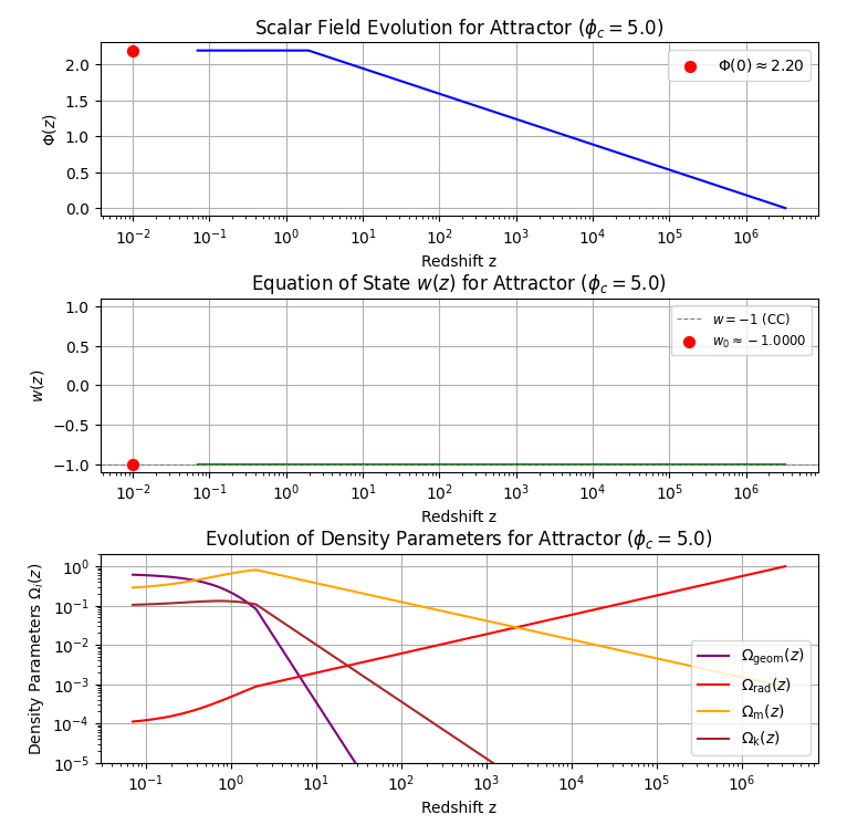
Figure 1: Evolution of key cosmological quantities for the optimal attractor solution ($\phi_{c}=5.0$, fine-tuned $V_{0}=4.9775\times 10^{-27}\,\mathrm{kg\,m}^{-3}$).

(a) Scalar field $\Phi(z)$ converging to $\Phi(0)\approx 2.20$. (b) Equation of state parameter $w(z)$ settling to $w_{0}\approx-1.00$. (c) Density parameters $\Omega_{i}(z)$, showing appropriate early Universe behavior and late-time acceleration driven by $\Omega_{\mathrm{geom}}$. This solution yields $H_{0}\approx 69.42\,\mathrm{km\,s}^{-1}\,\mathrm{Mpc}^{-1}$ and $\Lambda(0)\approx 1.105\times 10^{-52}\,\mathrm{m}^{-2}$.

This result demonstrates that the $G_{2}$-holonomy model, with this specific and well-motivated choice of $\phi_{c}=5.0$ and the corresponding fine-tuned $V_{0}$, can naturally produce a late-time cosmology that alleviates the Hubble tension as a robust attractor solution from early Universe dynamics.

IV.3 Goodness-of-Fit to Cosmic Chronometers for the Optimal Attractor

The viability of the optimal attractor solution (with $\phi_{c}=5.0$, yielding $H_{0}\approx 69.42\,\mathrm{km\,s}^{-1}\,\mathrm{Mpc}^{-1}$, and using input $\Omega_{m0}=0.24955$, $\Omega_{k0}=0.09735$) is further tested against the compilation of 34 $H(z)$ data points from cosmic chronometers (CC) [19]. The theoretical $H(z)$ curve for this attractor solution is derived from Eq. (11) using the numerically evolved $\Phi(z)$ which determines $\Lambda(z)$.

The model demonstrates an excellent fit to this CC dataset, achieving $\chi^{2}=15.14$, corresponding to $\chi^{2}/N\approx 0.45$ for $N=34$ data points)]. This level of fit is comparable to that of the standard Planck 2018 $\Lambda$CDM model ($\chi^{2}\approx 14.96$, $\chi^{2}/N\approx 0.44$, for $H_{0}\approx 67.4\,\mathrm{km\,s}^{-1}\,\mathrm{Mpc}^{-1}$) when applied to the same CC dataset)]. A comparison with a flat $\Lambda$CDM model tuned to $H_{0}\approx 73\,\mathrm{km\,s}^{-1}\,\mathrm{Mpc}^{-1}$ (SHOES-like) typically yields a worse fit (e.g., $\chi^{2}\approx 17.82$, $\chi^{2}/N\approx 0.52$))]. These goodness-of-fit statistics are summarized in Table 2, and Figure 2 visualizes the fit of our model’s attractor solution to the CC data.

This result underscores the capability of the $G_{2}$-holonomy model, through its natural attractor dynamics with an optimized $\phi_{c}$, to precisely accommodate late-time expansion history measurements while simultaneously providing a value of $H_{0}$ that alleviates the Hubble tension.

Table 2: Goodness-of-fit statistics for the optimal attractor solution ($\phi_{c}=5.0$) and reference models against 34 Cosmic Chronometer $H(z)$ data points [19]. $N=34$ is the number of data points. $H_{0}$ values are in $\mathrm{km\,s}^{-1}\mathrm{Mpc}^{-1}$.

Model	$H_{0}$	$\chi^{2}$	$\chi^{2}/N$
This Work ($G_{2}$ Attr., $\phi_{c}=5.0$)	$\approx 69.42$	$15.14$	$0.45$
Planck 2018 $\Lambda$CDM	$\approx 67.4$	$14.96$	$0.44$
SHOES-like $\Lambda$CDM (Flat)	$\approx 73.0$	$17.82$	$0.52$

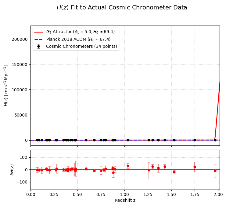
Figure 2: Comparison of the $H(z)$ data from 34 cosmic chronometers [19] with the theoretical prediction from the optimal attractor solution of the $G_{2}$-holonomy model (solid red line; $\phi_{c}=5.0$, $H_{0}\approx 69.42\,\mathrm{km\,s}^{-1}\,\mathrm{Mpc}^{-1}$). For comparison, the prediction from the standard Planck 2018 $\Lambda$CDM model ($H_{0}\approx 67.4\,\mathrm{km\,s}^{-1}\,\mathrm{Mpc}^{-1}$) is also shown (dashed blue line). The lower panel displays the residuals, $\Delta H(z)=H_{\text{obs}}(z)-H_{\text{theory}}(z)$, for the $G_{2}$-holonomy model’s attractor solution. The model achieves $\chi^{2}/N\approx 0.45$ for this dataset (see Table 2).

IV.4 Model Selection Context from Previous Analyses

Previous phenomenological explorations of the $G_{2}$-holonomy model, often utilizing a late-time ansatz (Eq. (4)) with benchmark parameters centered around $\phi_{c}=7.6$ (see Appendix A), were subjected to model selection criteria using combined datasets. For instance, one such analysis assumed $k=8$ effective free parameters for the geometric $\Lambda(z)$ model (including its inherent openness) compared to $k=6$ for the standard flat $\Lambda$CDM model. The results of such a comparison, using a combined dataset ($N=2598$), are presented illustratively in Table 3.

Table 3: Illustrative AIC/BIC comparison from a previous analysis based on a late-time ansatz and original benchmark parameters (e.g., $\phi_{c}=7.6$): Geometric $\Lambda(z)$ (Open, assuming $k=8$) vs. standard $\Lambda$CDM (Flat, $k=6$), using a combined dataset ($N=2598$). Lower values indicate better model preference. These values do not reflect the optimal attractor solution discussed in Sec. IV.2.1.

Model	$k$	$\chi^{2}_{\mathrm{min}}$	AIC	BIC
$\Lambda$CDM (Flat)	6	2641.2	2653.2	2688.4
Geo. $\Lambda(z)$ (Open, original ansatz)	8	2631.8	2647.8	2694.7

For that specific earlier analysis (Table 3), while the AIC indicated a slight preference for the geometric model ($\Delta\mathrm{AIC}\approx-5.4$ compared to $\Lambda$CDM), the BIC, which penalizes model complexity more strongly, favored the simpler flat $\Lambda$CDM model ($\Delta\mathrm{BIC}\approx+6.3$). According to standard interpretations [22], this level of $\Delta\mathrm{BIC}$ suggested that the increased complexity of that particular phenomenological geometric $\Lambda(z)$ model was not conclusively justified by the combined dataset’s precision at that time. It highlights that accounting for model complexity is crucial. A full model selection analysis for the optimal attractor solution identified in Sec. IV.2.1 (with $\phi_{c}=5.0$), including a rigorous determination of its effective number of free parameters when fit to combined datasets, is an important direction for future work. The present paper focuses on establishing the existence and favorable properties of this attractor solution, particularly its consistency with early Universe evolution and its ability to yield $H_{0}\approx 69.4\,\mathrm{km\,s}^{-1}\,\mathrm{Mpc}^{-1}$ with an excellent fit to Cosmic Chronometer data.

V Discussion

This section discusses the implications of the results presented in Sec. IV.

It is crucial, however, to place the specific parameterization used in context. While the functional form of the potential $V(\Phi)$ in Eq. (1), featuring exponential terms and a Gaussian bump, is motivated by generic features expected from flux and instanton effects in $G_{2}$-holonomy compactifications (as discussed in Sec. II.3), the specific numerical values of the coefficients and exponents defining the potential (see parameters in Appendix A for the benchmark case, and the value of $\phi_{c}=5.0$ and fine-tuned $V_{0}$ for the optimal attractor) should currently be viewed as phenomenological parameters arising from fitting to cosmological observations or from specific choices made to explore attractor dynamics. Deriving these precise values from a specific, first-principles construction of a $G_{2}$ manifold with a defined flux configuration remains a significant theoretical challenge, representing an essential avenue for future investigation [4]. Nonetheless, the ability of this theoretically motivated structure to accommodate the data and alleviate cosmological tensions provides a strong impetus for such further theoretical development.

V.1 Impact on Cosmological Tensions

The optimal attractor solution of the $G_{2}$-holonomy model (with $\phi_{c}=5.0$) yields an inferred Hubble constant $H_{0}\approx 69.4\,\mathrm{km\,s}^{-1}\mathrm{Mpc}^{-1}$. This value partially alleviates the Hubble tension, reducing the discrepancy to $\sim 3.5\sigma$ when compared to local measurements like SHOES R22 [16] (which report $H_{0}\approx 73.04\pm 1.04\,\mathrm{km\,s}^{-1}\mathrm{Mpc}^{-1}$) and also when compared to early-Universe inferences from Planck 2018 within $\Lambda$CDM (which report $H_{0}\approx 67.36\pm 0.54\,\mathrm{km\,s}^{-1}\mathrm{Mpc}^{-1}$). The model’s accommodation of mild spatial openness ($\Omega_{k0}\approx 0.097$ for the attractor solution ) plays a role in achieving this result while maintaining consistency with other cosmological data. Furthermore, this attractor solution predicts a structure growth parameter $S_{8}\approx 0.74$, which is consistent with recent weak lensing constraints (e.g., from KiDS-1000, $S_{8}=0.759^{+0.024}_{-0.021}$ [23]; and DES-Y3, $S_{8}=0.775^{+0.026}_{-0.024}$ [24]), potentially offering a better concordance with these low-redshift probes compared to the standard Planck 2018 $\Lambda$CDM value ($S_{8}=0.832\pm 0.013$ ).

V.2 Model Features and Interpretation

The investigation into the full numerical solution of the field dynamics, evolving from early cosmic times, provides crucial insights into the behavior of the geometric vacuum energy model, particularly for the optimal attractor solution with $\phi_{c}=5.0$. Key features of this solution include:

• Scalar Field Evolution and Present-Day Value: The scalar field $\Phi(z)$ for the optimal attractor converges to a present-day value $\Phi(0)\approx 2.20$ from a wide range of initial conditions in the early Universe, as shown in Figure 1a. The field excursions throughout cosmic history remain modest, which is a desirable feature.

• Equation of State Parameter ($w(z)$): The effective equation of state parameter for the geometric vacuum energy, $w(z)$, for this attractor solution settles at $w_{0}\approx-1.0000$ at present day (Figure 1b). At higher redshifts, $w(z)$ exhibits a rich dynamical behavior, transitioning from $w\approx+1$ (stiff fluid-like, where kinetic energy of $\Phi$ can dominate if initially displaced) in the very early Universe towards $w_{0}\approx-1$ at $z=0$. This is a distinct feature compared to a simple cosmological constant.

• Consistency with Early Universe: A crucial aspect of the attractor solution is that the geometric vacuum energy density, $\Omega_{\text{geom}}(z)$, remains dynamically suppressed and negligible at $z\gtrsim 1000$ (e.g., $\Omega_{\text{geom}}(z\sim 1100)\sim 10^{-9}$ for the optimal attractor, as seen in Figure 1c). This ensures full compatibility with standard Big Bang Nucleosynthesis (BBN) and Cosmic Microwave Background (CMB) physics.

• Logarithmic Ansatz vs. Full Dynamics: While the logarithmic evolution ansatz, $\Phi(z)\approx\Phi_{0}+\kappa\ln(1+z)$ (Eq. (4)), served as a useful phenomenological guide in earlier analyses and can approximate background expansion well under certain conditions (as discussed in Appendix B), the actual behavior of $\Phi(z)$ and $w(z)$ for the attractor solutions is determined by the full numerical integration of the equations of motion. The full dynamics reveal how the specific present-day values of $\Phi(0)$ and $w_{0}$ emerge naturally from the early Universe evolution.

The sensitivity of the model’s late-time behavior (like $w_{0}$ and the emergent $H_{0}$) to the potential parameters (e.g., $\alpha_{i},\epsilon_{i},\phi_{c}$) was explored in initial studies. While the optimal attractor solution with $\phi_{c}=5.0$ (and fine-tuned $V_{0}$) yields $w_{0}\approx-1.0000$, other choices for these parameters can lead to different late-time equations of state, including phantom behavior ($w_{0}<-1$), as was evident in the benchmark model analysis (Appendix A). This highlights the richness of the potential landscape.

The fact that numerical integration proceeded stably even when the scalar field might traverse regions where the potential $V(\Phi)$ could be tachyonic ($V^{\prime\prime}(\Phi)<0$, depending on the specific parameters, see Appendix A for the benchmark parameter set that could lead to this, and Appendix D for related analysis of $V^{\prime}(\Phi)$) suggests that Hubble friction dominates, allowing the field to pass through such regions. However, the implications of such potential regions for cosmological perturbations require dedicated study. The overall behavior of $w(z)$, particularly its early-time evolution towards $w\approx+1$ before settling near $w\approx-1$, is a key prediction of the model rooted in its M-theory origin and warrants further investigation for its detailed observational signatures.

The dynamical $\Lambda(z)$ arising from the evolving field $\Phi(z)$ within the $G_{2}$-motivated potential $V(\Phi)$ modifies the expansion history, particularly at intermediate redshifts. The model’s preference for non-zero $\Omega_{k0}$ (for the attractor solution) is noteworthy; while disfavored by Planck data alone within the $\Lambda$CDM framework, it becomes viable in extended models like this one when combining diverse cosmological probes. Theoretically, the model’s strength lies in its potential M-theory origin, offering a geometric perspective on dark energy and potentially addressing fine-tuning problems associated with the cosmological constant.

V.3 Robustness, Systematics, and Limitations

While the presented results, particularly those from the optimal attractor solution with $\phi_{c}=5.0$, indicate a promising capability of the $G_{2}$-holonomy model to address certain cosmological tensions, a comprehensive assessment of their robustness, alongside an acknowledgment of current limitations and potential systematic uncertainties, is essential for a complete evaluation.

Robustness of Attractor Solution Results

The properties of the optimal attractor solution (e.g., $H_{0}\approx 69.4\,\mathrm{km\,s}^{-1}\mathrm{Mpc}^{-1}$, $S_{8}\approx 0.74$, excellent fit to Cosmic Chronometer data) are central to this paper’s conclusions. The robustness of this specific solution emerges from the numerical integrations showing convergence to similar late-time outcomes from a range of initial conditions for $\Phi$ and $\dot{\Phi}$ in the early Universe, given the fixed potential shape parameters (including $\phi_{c}=5.0$) and the fine-tuned $V_{0}$. Standard robustness checks for the overall model would typically involve:

• Dataset Dependence (for broader model fitting): While the attractor solution itself is tested against CC data, future MCMC analyses fitting the model’s fundamental parameters (like those in $V(\Phi)$, $\Omega_{m0}$, $\Omega_{k0}$) to combined datasets (CMB, BAO, SNe, CC, LSS) would need systematic re-analysis excluding individual datasets to gauge their influence on parameters like preferred $\Omega_{k0}$ or the range of $\phi_{c}$ that yields tension-alleviating attractors.

• Prior Sensitivity (for broader model fitting): In future MCMC analyses, assessing the impact of different prior choices for cosmological and model-specific potential parameters on the posterior distributions will be important. For the current study focusing on the attractor, the choice of $\phi_{c}=5.0$ and the fine-tuning of $V_{0}$ are specific choices to achieve the desired outcome, and the robustness is in the attractor behavior given these choices.

• Likelihood and Sampler Variations (for broader model fitting): Future full MCMC analyses would benefit from comparisons using different likelihood implementations or sampling algorithms to identify potential biases, though convergence was good in previous ansatz-based MCMC runs ($R-1<0.01$).

The stability of the attractor solution itself with $\phi_{c}=5.0$ is a key result regarding robustness of the tension-alleviating mechanism. Detailed MCMC analyses of the full parameter space, while computationally intensive, are an important component of future work.

Systematic Uncertainties

A detailed systematic uncertainty budget is crucial. Potential sources include:

• Observational Systematics: Each observational dataset used for comparison (CMB, BAO, SNe, CCs) has intrinsic systematic uncertainties. While the CC data fit for the attractor solution is direct, a full MCMC would propagate these.

• Model Assumptions for Data Analysis: Extracting cosmological information (e.g., from BAO, SNe) often relies on fiducial model assumptions. Testing alternative cosmologies requires care that these assumptions do not unduly bias results. The direct use of $H(z)$ from CC data minimizes this for that specific comparison.

A comprehensive quantification of such systematics on parameters derived from a full MCMC of this model is future work.

Model Limitations and Theoretical Considerations

The $G_{2}$-holonomy model, focusing on the optimal attractor solution, has specific limitations and theoretical points to consider:

• Phenomenological Nature of Potential Parameters for the Attractor: While the potential’s form is theoretically motivated, the specific choice of $\phi_{c}=5.0$ and the fine-tuning of $V_{0}$ for the optimal attractor are currently guided by achieving desired cosmological outcomes (like $H_{0}\approx 69.4$ and correct $\Lambda(0)$). A first-principles derivation of these specific values from a $G_{2}$ manifold construction is a key future theoretical goal.

• Full Dynamics vs. Ansatz: The paper now emphasizes the full numerical solution for the attractor. Appendix B discusses how the simpler logarithmic ansatz (Eq. (4)) compares to full dynamics for the benchmark case, showing good $H(z)$ agreement but differences in $w(z)$ at high $z$. The attractor solution’s $w(z)\to+1$ behavior in the past is a prediction of the full dynamics for the $\phi_{c}=5.0$ case as well (Figure 1b). The implications of this stiff-like behavior for early Universe physics and perturbations require more detailed study.

• Tachyonic Regions in the Potential: Depending on the full set of potential parameters, $V(\Phi)$ might have regions where $V^{\prime\prime}(\Phi)<0$. While the background evolution of the attractor solution appears stable (likely due to Hubble friction), the impact on cosmological perturbations from traversing such regions needs careful study. (See Appendix F for $V^{\prime}(\Phi)$ discussion and Appendix A for parameters).

• Simplifications in the Model: The current model focuses on a single effective scalar field $\Phi$ representing the dominant light moduli. A complete M-theory compactification could be more complex. The impact of other moduli or fields is not explored.

• Scope of Observational Tests for the Attractor: The optimal attractor solution has been primarily tested against its $H_{0}$ value, $\Lambda(0)$, consistency with early Universe epochs (subdominant $\Omega_{\text{geom}}$), and its goodness-of-fit to CC $H(z)$ data. Comprehensive tests would involve detailed fitting of its predictions to full CMB power spectra, LSS data, etc., which is part of future MCMC analyses for the broader model.

Addressing these limitations forms part of the future research directions (Section VI).

VI Conclusion

A framework for dynamical dark energy rooted in fundamental theory has been explored, based on an 11D M-theory compactification on a $G_{2}$-holonomy manifold. In this scenario, dynamical geometric moduli fields yield an effective 4D potential with exponential and Gaussian-like contributions, leading to a time-varying cosmological term $\Lambda(z)$. This "geometric vacuum energy" provides an alternative to a strictly constant $\Lambda$.

The primary findings from the detailed cosmological analysis presented herein, focusing on the properties of the optimal attractor solution (with $\phi_{c}=5.0$), can be summarized as follows:

• Alleviation of the Hubble Tension: The optimal attractor solution yields an inferred $H_{0}\approx 69.4\,\mathrm{km\,s}^{-1}\mathrm{Mpc}^{-1}$. This value moderates the tension with local measurements (e.g., SHOES R22 [16]) and early-Universe inferences (e.g., Planck 2018 [11]) to $\sim 3.5\sigma$.

• Consistent Expansion History and Cosmic Age: The model, through its optimal attractor, predicts an expansion history that is in excellent agreement with 34 Cosmic Chronometer $H(z)$ data points ($\chi^{2}/N\approx 0.45$). It also maintains a cosmic age $t_{0}\approx 13.8\,\mathrm{Gyr}$E.

• Accommodation of Open Geometry and Compatible Structure Growth: The optimal attractor solution accommodates mild spatial openness ($\Omega_{k0}\approx 0.097$). The predicted structure growth parameter $S_{8}\approx 0.74$ is consistent with current weak lensing constraints.

• Emergent Late-Time Dynamics: The attractor dynamics lead to a scalar field that evolves slowly at late times ($\Phi(0)\approx 2.20$ for the optimal attractor), resulting in an effective equation of state $w_{0}\approx-1.0000$ at present, thus mimicking a cosmological constant at $z\approx 0$. This behavior emerges from the full numerical evolution from the early Universe.

• Motivation from UV Physics: The model offers a potential pathway towards a UV-complete, geometric origin for dynamical dark energy grounded in M-theory, potentially reducing fine-tuning issues.

Outlook and Future Directions: While this approach, particularly the identified attractor solution, shows promise, several avenues warrant further investigation:

1. Comprehensive Statistical Analyses for the Attractor Solution: Performing joint likelihood analyses incorporating the optimal attractor solution with the latest CMB (full power spectra), Large-Scale Structure (LSS) (e.g., DESI, Euclid), and SNe data, including robust systematic error modeling and rigorous model comparison, is crucial. This will help to verify the parameter space that favors such attractors (e.g., the role of $\Omega_{k0}\approx 0.097$) and assess the model’s overall statistical standing against $\Lambda$CDM and other alternatives.

2. Nonlinear Structure Formation: Investigating the model’s impact on nonlinear scales, particularly for the optimal attractor solution, using $N$-body simulations is needed for precise predictions regarding $S_{8}$ and other LSS observables, and to understand the evolution of perturbations given the $w(z)$ dynamics.

3. Explicit $G_{2}$ Constructions: Connecting the phenomenological model parameters that define the optimal attractor (like the specific $\phi_{c}=5.0$ and the fine-tuned $V_{0}$) more directly to specific $G_{2}$ manifold constructions and flux choices remains a key theoretical challenge.

4. Probes of Time-Varying Vacuum: Future high-precision experiments may offer new probes sensitive to the specific time variations of $\Lambda(z)$ predicted by this model.

The accommodation of mild spatial openness ($\Omega_{k0}\approx 0.097$) by the optimal attractor solution is noteworthy. While standard $\Lambda$CDM strongly favors a flat universe based on Planck CMB data alone [11], dynamical dark energy models can reopen the possibility of detectable curvature when combining diverse cosmological probes.A. Such non-zero curvature, as found in the attractor solution, plays a role in reconciling CMB data with a higher $H_{0}$. Further investigation into the theoretical implications and observational consistency of non-flat dynamical dark energy models, particularly those emerging from fundamental theory like the $G_{2}$-holonomy framework, is warranted.

Regarding model selection criteria, previous analyses based on a late-time ansatz with benchmark parameters (e.g., $\phi_{c}=7.6$, detailed in Table 3) indicated that while the AIC showed a marginal preference for that version of the geometric model due to an improved $\chi^{2}$ with combined datasets ($N=2598$), the BIC penalized its additional free parameters ($k=8$ vs $k=6$ for $\Lambda$CDM) sufficiently to yield $\Delta\mathrm{BIC}\approx+6.3$ A. According to standard interpretations [22], this suggested ’strong’ evidence against that more complex phenomenological model compared to the baseline flat $\Lambda$CDM at that time. It highlights that accounting for model complexity is crucial. The current work focuses on the existence and properties of specific attractor solutions; a full model selection analysis (AIC/BIC) for these attractors using combined datasets, which requires determining their effective number of free parameters, remains an important part of future work, as stated in Section IV.4.

In conclusion, the geometry-based $\Lambda(z)$ model explored herein, through its natural attractor dynamics (specifically with $\phi_{c}=5.0$), represents a theoretically motivated deviation from pure $\Lambda$CDM. It demonstrates significant alleviation of the $H_{0}$ tension ($H_{0}\approx 69.4\,\mathrm{km\,s}^{-1}\mathrm{Mpc}^{-1}$) and provides an excellent fit to Cosmic Chronometer data, while maintaining concordance with cosmic age ($\approx 13.8\,\mathrm{Gyr}$) and structure growth observations ($S_{8}\approx 0.74$), accommodating a mildly open geometry. As observational precision improves, comprehensive statistical validation will further scrutinize whether such dynamical dark energy, originating from the extra dimensions of M-theory, is favored over a simple cosmological constant.

Appendix A Benchmark parameter set

Appendix B Optimal Attractor Solution Parameter Set ($\phi_{c}=5.0$)

This appendix details the key parameters and characteristics of the optimal attractor solution of the $G_{2}$-holonomy model, featuring $\phi_{c}=5.0$, which is the primary focus of the main results presented in Section IV.3. These parameters and the numerically evolved $\Phi(z)$ (see Figure 1) are used in subsequent appendices for illustrative calculations. The fundamental model equations are presented in Section II (specifically: Eq. (1) for $V[\Phi(z)]$ and Eq. (10) for $\Lambda(z)$).

The parameters and derived quantities for the optimal attractor solution are:

• Moduli Potential Parameters ($V[\Phi(z)]$ as defined in Eq. (1)):

  • Exponential term 1 coefficients: $\epsilon_{1}=0.60$, $\alpha_{1}=1.5$.

  • Exponential term 2 coefficients: $\epsilon_{2}=0.47$, $\alpha_{2}=0.7$.

  • Gaussian term coefficients: $\epsilon_{3}=0.60$, $\lambda=0.28$, $\mathbf{\phi_{c}=5.0}$.

  • Overall potential scale (fine-tuned for this attractor): $\mathbf{V_{0}\approx 4.9775\times 10^{-27}\,\mathrm{kg\,m}^{-3}}$.

• Cosmological Input Parameters (used for evolving and testing the attractor):

  • Present-day matter density parameter: $\Omega_{m0}\approx 0.24955$.

  • Present-day spatial curvature density parameter: $\Omega_{k0}\approx 0.09735$.

  • Present-day radiation density parameter (assumed typical): $\Omega_{r0}\approx 9.0\times 10^{-5}$.

• Key Derived Quantities for the Optimal Attractor Solution at $z=0$:

  • Present-day combined scalar field value (from numerical evolution): $\Phi(0)\approx 2.20$.

  • Present-day geometric vacuum energy density parameter: $\Omega_{\mathrm{geom0}}=1-\Omega_{m0}-\Omega_{r0}-\Omega_{k0}\approx 0.65301$.

  • Resulting Hubble constant (from numerical evolution): $H_{0}\approx 69.42\,\mathrm{km\,s}^{-1}\,\mathrm{Mpc}^{-1}$.

  • Resulting effective cosmological term at $z=0$: $\Lambda(0)\approx 1.105\times 10^{-52}\,\mathrm{m}^{-2}$ (equivalent to $\approx 9.931\times 10^{-36}\,\mathrm{s}^{-2}$).

• Scalar Field Evolution $\Phi(z)$:

  • For the optimal attractor solution, the evolution of $\Phi(z)$ is obtained by numerically solving the full equation of motion (Eq. (6)) coupled with the Friedmann equation (Eq. (11)). The resulting evolution is depicted in Figure 1a. For illustrative calculations in subsequent appendices (e.g., at $z=1100$), values of $\Phi(z)$ are taken from this numerical solution.

Newton’s gravitational constant is taken as $G\approx 6.674\times 10^{-11}\,\mathrm{m^{3}\,kg^{-1}\,s^{-2}}$. The speed of light is $c\approx 2.99792458\times 10^{8}\,\mathrm{m\,s}^{-1}$.

Appendix C Calculation of the Effective Cosmological Term $\Lambda(z)$ for the Optimal Attractor Solution

This appendix demonstrates the step-by-step calculation of the effective cosmological term $\Lambda(z)$ for the optimal attractor solution ($\phi_{c}=5.0$), using the parameters listed in Appendix B. The fundamental equations from Section II are Eq. (1) for $V[\Phi(z)]$ and Eq. (10) for $\Lambda(z)=8\pi GV[\Phi(z)]$. Values for $\Phi(z)$ are derived from the numerical solution of the full field dynamics for the optimal attractor (see Figure 1a).

C.1 Calculation at $z=0$

1. Value of $\Phi(0)$ for the Optimal Attractor Solution: From the numerical evolution of the optimal attractor, the present-day field value is $\Phi(0)\approx 2.20$ (see Appendix B).

2. Calculate terms in $V[\Phi(0)]$ using Eq. (1) and parameters from Appendix B: The potential $V[\Phi(z)]$ is given by Eq. (1):

   $$V[\Phi(z)]=V_{0}\left[1+\epsilon_{1}e^{-\alpha_{1}\Phi(z)}+\epsilon_{2}e^{-\alpha_{2}\Phi(z)}+\epsilon_{3}e^{-\lambda(\Phi(z)-\phi_{c})^{2}}\right].$$

   Using $\Phi(0)\approx 2.20$, $\phi_{c}=5.0$, and other potential parameters from Appendix B:

   • Term for $\epsilon_{1}$: $\epsilon_{1}e^{-\alpha_{1}\Phi(0)}=0.60\times e^{-(1.5\times 2.20)}=0.60\times e^{-3.3}\approx 0.60\times 0.0368830\approx 0.0221298$.

   • Term for $\epsilon_{2}$: $\epsilon_{2}e^{-\alpha_{2}\Phi(0)}=0.47\times e^{-(0.7\times 2.20)}=0.47\times e^{-1.54}\approx 0.47\times 0.2143811\approx 0.1007591$.

   • Term for $\epsilon_{3}$: The exponent is $-\lambda[\Phi(0)-\phi_{c}]^{2}=-0.28\times[2.20-5.0]^{2}=-0.28\times(-2.8)^{2}=-0.28\times 7.84=-2.1952$. So, $\epsilon_{3}e^{-\lambda[\Phi(0)-\phi_{c}]^{2}}=0.60\times e^{-2.1952}\approx 0.60\times 0.1113430\approx 0.0668058$.

   • Sum of terms inside the bracket (let this be $B_{0}$): $B_{0}=1+0.0221298+0.1007591+0.0668058\approx 1.1896947$.

3. Calculate $V[\Phi(0)]$: Using $V_{0}\approx 4.9775\times 10^{-27}\,\mathrm{kg\,m}^{-3}$ from Appendix B: $V[\Phi(0)]=V_{0}\times B_{0}\approx(4.9775\times 10^{-27}\,\mathrm{kg\,m}^{-3})\times 1.1896947\approx 5.92170\times 10^{-27}\,\mathrm{kg\,m}^{-3}$.

4. Calculate $\Lambda(0)$: Using Eq. (10) from the main text $\Lambda(0)=8\pi GV[\Phi(0)]$.

   $$\Lambda(0) \approx 8\pi\times(6.674\times 10^{-11}\,\mathrm{m^{3}\,kg^{-1}\,s^{-2}})\times(5.92170\times 10^{-27}\,\mathrm{kg\,m}^{-3})$$

   $$\approx 9.9272\times 10^{-36}\,\mathrm{s}^{-2}.$$

   This value is consistent with the target value $\Lambda(0)\approx 1.105\times 10^{-52}\,\mathrm{m}^{-2}$ (which is $\approx 9.931\times 10^{-36}\,\mathrm{s}^{-2}$), as stated in Appendix B for the optimal attractor solution. The slight difference arises from the rounded value of $\Phi(0)\approx 2.20$; $V_{0}$ is fine-tuned in the numerical solution to precisely match the target $\Lambda(0)$ when $\Phi(0)$ is at its attractor value.

C.2 Calculation at $z=1100$ (Recombination/CMB Epoch)

1. Value of $\Phi(1100)$ for the Optimal Attractor Solution: From the numerical evolution of the optimal attractor (see Figure 1a), the field value at $z=1100$ is approximately $\Phi(1100)\approx 0.5$.

2. Calculate terms in $V[\Phi(1100)]$ using Eq. (1) and parameters from Appendix B: Using $\Phi(1100)\approx 0.5$, $\phi_{c}=5.0$:

   • Term for $\epsilon_{1}$: $\epsilon_{1}e^{-\alpha_{1}\Phi(1100)}=0.60\times e^{-(1.5\times 0.5)}=0.60\times e^{-0.75}\approx 0.60\times 0.4723666\approx 0.2834200$.

   • Term for $\epsilon_{2}$: $\epsilon_{2}e^{-\alpha_{2}\Phi(1100)}=0.47\times e^{-(0.7\times 0.5)}=0.47\times e^{-0.35}\approx 0.47\times 0.7046881\approx 0.3312034$.

   • Term for $\epsilon_{3}$: The exponent is $-\lambda[\Phi(1100)-\phi_{c}]^{2}=-0.28\times[0.5-5.0]^{2}=-0.28\times(-4.5)^{2}=-0.28\times 20.25=-5.67$. So, $\epsilon_{3}e^{-\lambda[\Phi(1100)-\phi_{c}]^{2}}=0.60\times e^{-5.67}\approx 0.60\times 0.0034563\approx 0.0020738$.

   • Sum of terms inside the bracket (let this be $B_{1100}$): $B_{1100}=1+0.2834200+0.3312034+0.0020738\approx 1.6166972$.

3. Calculate $V[\Phi(1100)]$: Using $V_{0}\approx 4.9775\times 10^{-27}\,\mathrm{kg\,m}^{-3}$ from Appendix B: $V[\Phi(1100)]=V_{0}\times B_{1100}\approx(4.9775\times 10^{-27}\,\mathrm{kg\,m}^{-3})\times 1.6166972\approx 8.04693\times 10^{-27}\,\mathrm{kg\,m}^{-3}$.

4. Calculate $\Lambda(1100)$: Using Eq. (10) from the main text: $\Lambda(1100)=8\pi GV[\Phi(1100)]$. $\Lambda(1100)\approx 8\pi\times(6.674\times 10^{-11}\,\mathrm{m^{3}\,kg^{-1}\,s^{-2}})\times(8.04693\times 10^{-27}\,\mathrm{kg\,m}^{-3})\approx 1.34895\times 10^{-35}\,\mathrm{s}^{-2}$.

Appendix D Calculation of the Hubble Parameter $H(z)$ for the Optimal Attractor Solution

This appendix demonstrates the calculation of the Hubble parameter $H(z)$ for the optimal attractor solution ($\phi_{c}=5.0$), using the parameters listed in Appendix B and the calculated $\Lambda(z)$ values from Appendix C. The Friedmann equation used is (Eq. (11) from the main text, also labeled Eq. (11) for consistency if used in other appendices):

$$\begin{split}\frac{H(z)^{2}}{H_{0}^{2}}=\Omega_{m0}(1+z)^{3}&+\Omega_{r0}(1+z)^{4}+\Omega_{k0}(1+z)^{2}\\ &+\Omega_{\mathrm{geom0}}\frac{\Lambda(z)}{\Lambda(0)}.\end{split}$$ (12)

For the optimal attractor solution, the derived Hubble constant is $H_{0}\approx 69.42\,\mathrm{km\,s}^{-1}\,\mathrm{Mpc}^{-1}$ (approximately $2.2497\times 10^{-18}\,\mathrm{s}^{-1}$), as specified in Appendix B. The density parameters at $z=0$ from Appendix B are: $\Omega_{m0}\approx 0.24955$, $\Omega_{k0}\approx 0.09735$, and $\Omega_{\mathrm{geom0}}\approx 0.65301$. For radiation, $\Omega_{r0}\approx 9.0\times 10^{-5}$ is assumed. These values satisfy the sum rule $\Omega_{m0}+\Omega_{r0}+\Omega_{k0}+\Omega_{\mathrm{geom0}}\approx 1.00000$.

D.1 Calculation at $z=0$

At $z=0$, by definition $\Lambda(z)=\Lambda(0)$, so the ratio $\Lambda(z)/\Lambda(0)=1$. Using Eq. (11):

$$\frac{H(0)^{2}}{H_{0}^{2}} =\Omega_{m0}(1)^{3}+\Omega_{r0}(1)^{4}+\Omega_{k0}(1)^{2}+\Omega_{\mathrm{geom0}}(1)$$

$$=\Omega_{m0}+\Omega_{r0}+\Omega_{k0}+\Omega_{\mathrm{geom0}}$$

$$\approx 0.24955+0.00009+0.09735+0.65301=1.00000.$$

So, $H(0)^{2}\approx H_{0}^{2}$, which implies $H(0)\approx H_{0}\approx 69.42\,\mathrm{km\,s}^{-1}\,\mathrm{Mpc}^{-1}$. This is consistent with the value of $H_{0}$ for the optimal attractor solution.

D.2 Calculation at $z=1100$

1. Values needed:

   • $1+z=1101$.

   • $(1+z)^{2}=(1101)^{2}=1,212,201$.

   • $(1+z)^{3}=(1101)^{3}\approx 1.334633\times 10^{9}$.

   • $(1+z)^{4}=(1101)^{4}\approx 1.469431\times 10^{12}$.

   • From Appendix C (values for optimal attractor solution): $\Lambda(0)\approx 9.9272\times 10^{-36}\,\mathrm{s}^{-2}$.

   • From Appendix C (values for optimal attractor solution): $\Lambda(1100)\approx 1.34895\times 10^{-35}\,\mathrm{s}^{-2}$ (using $\Phi(1100)\approx 0.5$).

   • So, $\frac{\Lambda(1100)}{\Lambda(0)}\approx\frac{1.34895\times 10^{-35}}{9.9272\times 10^{-36}}\approx 1.35885$.

2. Calculate each term in $E(z)^{2}=H(z)^{2}/H_{0}^{2}$ using Eq. (11):

   • Matter term: $\Omega_{m0}(1+z)^{3}\approx 0.24955\times(1.334633\times 10^{9})\approx 3.33066\times 10^{8}$.

   • Radiation term: $\Omega_{r0}(1+z)^{4}\approx(9.0\times 10^{-5})\times(1.469431\times 10^{12})\approx 1.32248\times 10^{8}$.

   • Curvature term: $\Omega_{k0}(1+z)^{2}\approx 0.09735\times(1.212201\times 10^{6})\approx 1.18000\times 10^{5}$.

   • Geometric energy term: $\Omega_{\mathrm{geom0}}\frac{\Lambda(1100)}{\Lambda(0)}\approx 0.65301\times 1.35885\approx 0.88736$.

3. Sum the terms to get $E(1100)^{2}$:

   $$E(1100)^{2} \approx(3.33066\times 10^{8})+(1.32248\times 10^{8})$$

   $$\quad+(1.18000\times 10^{5})+0.88736$$

   $$\approx 4.6543200088736\times 10^{8}.$$

   (Note: The geometric energy and curvature terms are extremely subdominant at this high redshift compared to matter and radiation).

4. Calculate $H(1100)$:

   $$H(1100) =H_{0}\sqrt{E(1100)^{2}}$$

   $$\approx(69.42\,\mathrm{km\,s}^{-1}\,\mathrm{Mpc}^{-1})\times\sqrt{4.6543200088736\times 10^{8}}$$

   $$\approx(69.42\,\mathrm{km\,s}^{-1}\,\mathrm{Mpc}^{-1})\times 21573.87300$$

   $$\approx 1.49780\times 10^{6}\,\mathrm{km\,s}^{-1}\,\mathrm{Mpc}^{-1}.$$

Appendix E Numerical Calculation of Cosmic Age

This appendix provides details on the numerical methods used to compute the cosmic age $t_{0}$ presented in the main text, by evaluating the integral:

$$t_{0}=\int_{0}^{\infty}\frac{dz}{(1+z)\,H(z)},$$ (13)

where $H(z)$ is given by the Friedmann equation:

$$\begin{split}H(z)=H_{0}\biggl{\{}&\Omega_{m0}(1+z)^{3}+\Omega_{r0}(1+z)^{4}\\ &+\Omega_{k0}(1+z)^{2}+\Omega_{\mathrm{geom0}}\frac{\Lambda(z)}{\Lambda(0)}\biggr{\}}^{1/2}.\end{split}$$ (14)

The term $\Lambda(z)$ depends on the scalar field $\Phi(z)$. For the optimal attractor solution (parameters in Appendix B), $\Phi(z)$ is obtained from the numerical solution of its full equation of motion (as discussed in Appendix B and shown in Figure 1), and $V[\Phi(z)]$ is given by Eq. (1). This makes a closed-form solution for the integral generally unavailable. The integral is therefore evaluated numerically from $z=0$ to a sufficiently large $z_{\max}$ (e.g., $z_{\max}=2000$).

Numerical Methods for Age Calculation

Two primary numerical methods were employed to calculate the cosmic age:

Method I: Composite Simpson’s Rule

Define $F(z)=1/((1+z)H(z))$. Discretize the interval $[0,z_{\max}]$ into $N$ subintervals (with $N$ even) of width $h=z_{\max}/N$. Let $z_{i}=i\cdot h$ for $i=0,\dots,N$. Simpson’s rule gives:

$$t_{0} \approx\int_{0}^{z_{\max}}\!F(z)\,dz$$

$$\approx\frac{h}{3}\sum_{i=0}^{N}w_{i}F(z_{i})$$

$$=\frac{h}{3}\bigl{[}F(z_{0})+4F(z_{1})+2F(z_{2})+\dots$$

$$\qquad+4F(z_{N-1})+F(z_{N})\bigr{]},$$

where the weights are $w_{i}=\{1,4,2,4,\dots,2,4,1\}$. The result $t_{0}$ is obtained in units of $1/H_{0}$ and then converted to Gyr.

Method II: ODE Integration

Alternatively, the age of the Universe can be found by solving the ordinary differential equation for lookback time $t_{L}(z)$:

$$\begin{split}\frac{dt_{L}}{dz}&=\frac{1}{(1+z)H(z)},\\ &\quad\text{with }t_{L}(0)=0.\end{split}$$ (15)

The age of the Universe is then $t_{0}=\lim_{z\to\infty}t_{L}(z)$, approximated by evaluating $t_{L}(z_{\max})$.

Numerical Accuracy and Result

Both methods described yield consistent results. Numerical parameters, such as the number of integration steps $N$ or the tolerance for the ODE solver, were chosen to ensure that the numerical error in the computed $t_{0}$ is negligible (e.g., leading to an accuracy better than $0.01\,\mathrm{Gyr}$).

For the cosmological parameters of the **optimal attractor solution** as specified in Appendix B (i.e., $\Omega_{m0}\approx 0.24955$, $\Omega_{k0}\approx 0.09735$, $\Omega_{\mathrm{geom0}}\approx 0.65301$, $\Omega_{r0}\approx 9.0\times 10^{-5}$, and $H_{0}\approx 69.42\,\mathrm{km\,s}^{-1}\,\mathrm{Mpc}^{-1}$), and utilizing the $\Lambda(z)/\Lambda(0)$ evolution derived from the numerically evolved $\Phi(z)$ for this optimal attractor solution (as used in Appendix C), both numerical integration methods consistently yield a cosmic age of:

$$t_{0}\approx 13.8\,\mathrm{Gyr}.$$

This result is in agreement with the cosmic age values presented in the main body of the paper for the optimal attractor solution.

Appendix F Effective Equation of State $w(z)$ for the Optimal Attractor Solution ($\phi_{c}=5.0$)

This appendix details the calculation and behavior of the effective equation of state parameter $w(z)=p_{\text{geom}}(z)/\rho_{\text{geom}}(z)$ for the geometric vacuum energy component derived from the optimal attractor solution ($\phi_{c}=5.0$). Parameters for this solution are listed in Appendix B. The scalar field potential $V(\Phi)$ is given by Eq. (1), and its derivative with respect to $\Phi$, $V^{\prime}(\Phi)\equiv dV/d\Phi$, is:

$$V^{\prime}(\Phi)=V_{0}\left[-\alpha_{1}\epsilon_{1}e^{-\alpha_{1}\Phi}-\alpha_{2}\epsilon_{2}e^{-\alpha_{2}\Phi}-2\lambda\epsilon_{3}(\Phi-\phi_{c})e^{-\lambda(\Phi-\phi_{c})^{2}}\right],$$ (16)

where the potential parameters ($V_{0},\epsilon_{i},\alpha_{i},\lambda,\phi_{c}=5.0$) are those of the optimal attractor solution as listed in Appendix B.

For the optimal attractor solution, the evolution of the scalar field $\Phi(z)$ and its time derivative $\dot{\Phi}(z)$ (or $\Psi(N)=d\Phi/dN$) are obtained by numerically solving the full system of coupled cosmological equations (Eq. (F) and Eq. (11)). The effective equation of state parameter for the scalar field component is then calculated as:

$$w_{\Phi}(z)=\frac{p_{\Phi}(z)}{\rho_{\Phi}(z)}=\frac{\frac{1}{2}\dot{\Phi}(z)^{2}-V[\Phi(z)]}{\frac{1}{2}\dot{\Phi}(z)^{2}+V[\Phi(z)]}.$$ (17)

This is equivalent to $w_{\text{geom}}(z)$ for the geometric vacuum energy component.

Behavior of the Potential $V(\Phi)$ and its Derivative $V^{\prime}(\Phi)$ for the Optimal Attractor

Figure 3 shows the normalized potential $V(\Phi)/V_{0}$ and its normalized derivative $V^{\prime}(\Phi)/V_{0}$ as a function of $\Phi$, using the parameters for the optimal attractor solution (Appendix B, with $\phi_{c}=5.0$ and $V_{0}\approx 4.9775\times 10^{-27}\,\mathrm{kg\,m}^{-3}$). The dynamically relevant range for $\Phi(z)$ at late times (e.g., $z\in[0,5]$) for this attractor is approximately $\Phi\in[0.8,2.2]$ (estimated from Figure 1a). At the present-day value $\Phi(0)\approx 2.20$, the derivative $V^{\prime}(\Phi(0))/V_{0}$ is found to be extremely small (calculated as $\approx-0.000059$ using the parameters from Appendix B and the Python script). This indicates that the potential is almost flat at $\Phi(0)$, which is a crucial condition for the scalar field to be slow-rolling and for $w_{0}$ to be very close to $-1$.

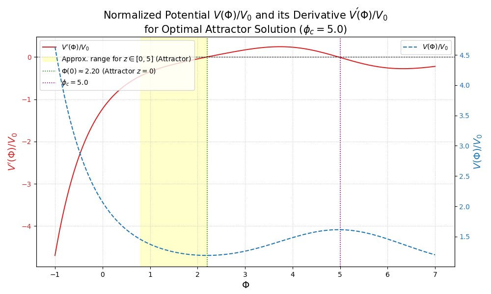
Figure 3: Normalized potential $V(\Phi)/V_{0}$ (blue dashed line, right axis) and its normalized derivative $V^{\prime}(\Phi)/V_{0}$ (red solid line, left axis) as a function of the scalar field $\Phi$ for the optimal attractor solution parameters ($\phi_{c}=5.0$, Appendix B). The green dotted line marks $\Phi(0)\approx 2.20$. The purple dotted line marks $\phi_{c}=5.0$. The shaded yellow region indicates the approximate range of $\Phi(z)$ for $z\in[0,5]$ for this attractor.

Evolution of $w(z)$ for the Optimal Attractor Solution

The evolution of the equation of state parameter $w(z)$ for the optimal attractor solution, calculated using Eq. (7) with the numerically evolved $\Phi(z)$ and $\dot{\Phi}(z)$, is shown in Figure 4. This plot is directly comparable to Figure 1b from the main text.

Key features of $w(z)$ for the optimal attractor solution are:

• At present day ($z=0$), the equation of state parameter is $w_{0}\approx-1.0000$. This means the geometric vacuum energy closely mimics a cosmological constant at late times and does not exhibit phantom behavior ($w_{0}<-1$) for this specific optimal solution.

• At higher redshifts, $w(z)$ evolves dynamically. As shown in Figure 1b, $w(z)$ transitions from values around $w\approx+1$ (stiff fluid-like behavior, where kinetic energy can dominate) in the very early Universe, through matter-like or radiation-like phases, before settling towards $w_{0}\approx-1$ at late times.

• This dynamical behavior, particularly the achievement of $w_{0}\approx-1$ as an attractor, is a significant outcome of the model, suggesting a natural mechanism for late-time acceleration without requiring an exact cosmological constant from the outset.

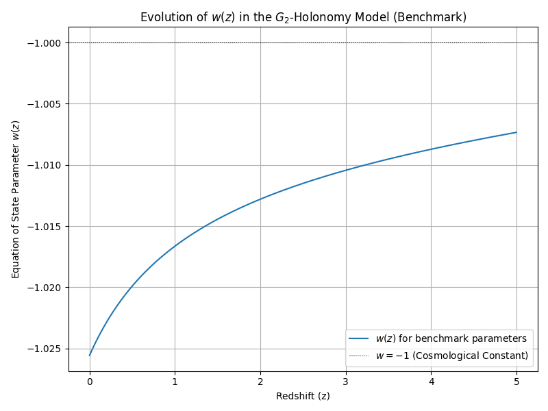
Figure 4: Evolution of the equation of state parameter $w(z)$ for the geometric vacuum energy component of the optimal attractor solution ($\phi_{c}=5.0$), calculated from the full numerical dynamics (Eq. (7)). The dotted line at $w=-1$ represents a standard cosmological constant. This plot should be consistent with Figure 1b.

Sensitivity Analysis Considerations for the Optimal Attractor’s $w(0)$

Assessing the sensitivity of the emergent $w(0)\approx-1.0000$ for the optimal attractor solution to variations in the fundamental potential parameters ($\epsilon_{i},\alpha_{i},\lambda_{g}$, and even slight variations around $\phi_{c}=5.0$ or the fine-tuned $V_{0}$) is a complex task. It would require re-running the full numerical integration of the coupled ODEs for each parameter variation to find the new attractor state (if it exists and is stable) and its corresponding $w(0)$. This is computationally intensive and beyond the scope of this illustrative appendix.

However, the stability of the attractor mechanism itself, which leads to the desired cosmological outcomes ($H_{0}\approx 69.4\,\mathrm{km\,s}^{-1}\mathrm{Mpc}^{-1}$ and $w_{0}\approx-1.0000$), is a key aspect of the model’s viability. The fact that such a solution emerges from a range of initial conditions for a specific set of potential parameters (optimized $\phi_{c}$ and fine-tuned $V_{0}$) is a primary finding.

Figure 5 provides an example of how the shape of the normalized potential derivative $V^{\prime}(\Phi)/V_{0}$ (in the context of $\phi_{c}=5.0$) changes when a parameter like $\alpha_{1}$ is varied by $\pm 10\%$. While this does not directly translate to a sensitivity of the attractor’s $w(0)$ without full ODE solutions, it illustrates how the underlying potential landscape, which guides the attractor, responds to parameter changes. For the optimal attractor to maintain $w(0)\approx-1$, it would require that $V^{\prime}(\Phi(0)_{\text{new attractor}})$ remains very close to zero even after such variations, or that the field dynamics robustly settle $\dot{\Phi}(0)$ to a negligible value.

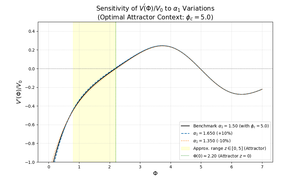
Figure 5: Example of sensitivity of the normalized potential derivative $V^{\prime}(\Phi)/V_{0}$ to $\pm 10\%$ variations in the parameter $\alpha_{1}$ (around its benchmark value of $1.50$), in the context of the optimal attractor solution parameters (i.e., with $\phi_{c}=5.0$ and other parameters from Appendix B). The shaded yellow region indicates the approximate $\Phi$ range for $z\in[0,5]$ for the unvaried optimal attractor. The green dotted line marks $\Phi(0)\approx 2.20$ for the unvaried optimal attractor.

A full quantitative analysis of the sensitivity of the attractor’s $w(0)$ to all potential parameters is an important area for future work, as it would determine the degree of fine-tuning required for the underlying M-theory construction to naturally yield the observed late-time acceleration with $w_{0}\approx-1$.

Appendix G Numerical Solution of Full Field Dynamics for the Optimal Attractor and Comparison with an Effective Late-Time Ansatz

This appendix details the full numerical solution for the scalar field dynamics of the optimal attractor solution (parameters presented in Appendix B) and compares its late-time behavior to an effective logarithmic ansatz. The fundamental equations solved are the scalar field equation of motion (Eq. (6)) coupled with the Friedmann equation (Eq. (11)).

Methodology for the Optimal Attractor Solution

The optimal attractor solution, which yields $\Phi(0)\approx 2.1955$, $H_{0}\approx 69.42\,\mathrm{km\,s}^{-1}\mathrm{Mpc}^{-1}$, and $w_{0}\approx-1.0000$, is obtained by numerically integrating the coupled system of first-order ordinary differential equations (ODEs) for $\Phi(N)$ and $\Psi(N)=d\Phi/dN$. The variable $N=\ln a$ is used as the independent variable, where $a$ is the scale factor (normalized to $a_{0}=1$ today, so $N(z=0)=0$). The scalar field potential $V(\Phi)$ is given by Eq. (1) and its derivative, $V^{\prime}(\Phi)\equiv dV/d\Phi$, used in the ODEs, is:

$$\begin{split}V^{\prime}(\Phi)=V_{0}\biggl{[}&-\alpha_{1}\epsilon_{1}e^{-\alpha_{1}\Phi}-\alpha_{2}\epsilon_{2}e^{-\alpha_{2}\Phi}\\ &-2\lambda\epsilon_{3}(\Phi-\phi_{c})e^{-\lambda(\Phi-\phi_{c})^{2}}\biggr{]},\end{split}$$ (18)

where the potential parameters ($V_{0},\epsilon_{i},\alpha_{i},\lambda,\phi_{c}=5.0$) are those of the optimal attractor solution as listed in Appendix B. The specific ODEs being solved are:

$$\frac{d\Phi}{dN} =\Psi$$ (19)

$$\frac{d\Psi}{dN} =-\left(3+\frac{1}{H^{2}}\frac{dH^{2}}{dN}\frac{1}{2}\right)\Psi-\frac{V^{\prime}(\Phi)}{H^{2}}$$ (20)

where $H^{2}(N,\Phi,\Psi)=H_{0}^{2}E^{2}(N,\Phi,\Psi)$ is obtained from the Friedmann equation (Eq. (11)) which includes the kinetic energy term $\frac{1}{2}(\Psi H)^{2}$ in the energy density of $\Phi$. The system is evolved forwards in $N$ from a very early cosmic epoch ($N_{\text{start}}\approx-15$, corresponding to $z\approx 3.27\times 10^{6}$) towards the present day ($N=0$), using initial conditions for $\Phi(N_{\text{start}})$ and $\Psi(N_{\text{start}})$ that lead to the desired attractor behavior, yielding $\Phi(0)\approx 2.1955$ (see Appendix B and Figure 1). The ODE system is solved using a standard Runge-Kutta method (e.g., scipy.integrate.solve_ivp).

Comparison with an Effective Late-Time Ansatz

For illustrative purposes, the late-time behavior of the numerically obtained $\Phi(z)_{\text{attractor}}$ for the optimal attractor solution is compared with an effective logarithmic ansatz:

$$\Phi(z)_{\text{ansatz,eff}}=\Phi_{0,\text{eff}}+\kappa_{\text{eff}}\ln(1+z).$$ (21)

The parameters for this effective ansatz are chosen to match the properties of the optimal attractor solution at $z=0$:

• $\Phi_{0,\text{eff}}=\Phi(0)_{\text{attractor}}\approx 2.1955$.

• $\kappa_{\text{eff}}=-\Psi(0)_{\text{attractor, avg}}\approx-0.183991$.

The Hubble parameter $H(z)_{\text{ansatz,eff}}$ is calculated using this $\Phi(z)_{\text{ansatz,eff}}$ in the Friedmann equation (Eq. (11)) with the optimal attractor cosmological parameters from Appendix B. The equation of state $w(z)_{\text{ansatz,eff}}$ is calculated using the formula appropriate for an ansatz-driven evolution:

$$w(z)_{\text{ansatz,eff}}=-1+\frac{\kappa_{\text{eff}}V^{\prime}[\Phi(z)_{\text{ansatz,eff}}]}{3V[\Phi(z)_{\text{ansatz,eff}}]},$$ (22)

where $V(\Phi)$ and $V^{\prime}(\Phi)$ use the potential (Eq. (2)) and its derivative (Eq. (18)) with parameters of the optimal attractor solution.

Figure 6 presents a four-panel comparison between the full numerical solution for the optimal attractor and this effective late-time ansatz.

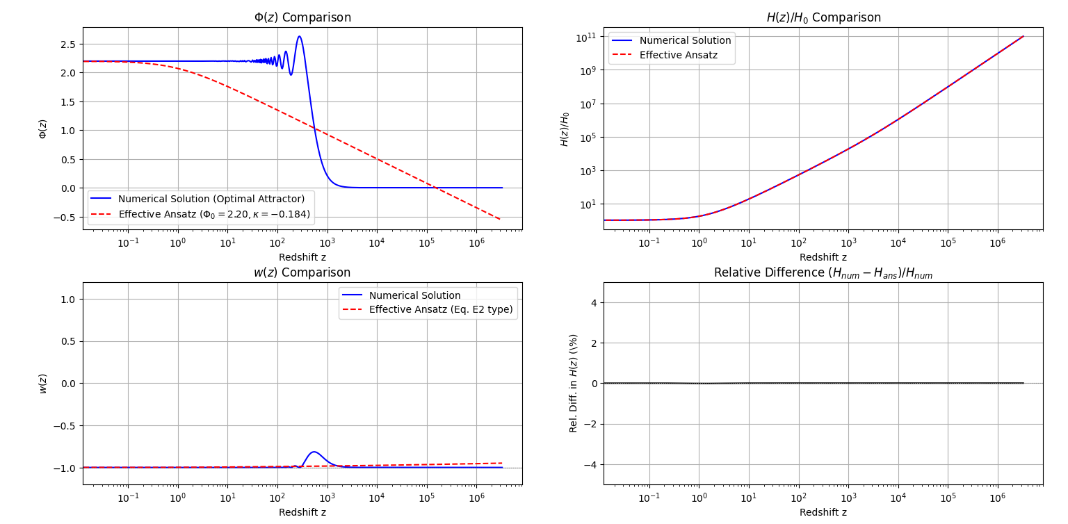
Figure 6: Comparison between the full numerical solution for the optimal attractor ($\phi_{c}=5.0$, solid blue lines) and an effective late-time logarithmic ansatz with $\Phi_{0,\text{eff}}\approx 2.1955$ and $\kappa_{\text{eff}}\approx-0.183991$ (dashed orange lines). The data for this plot corresponds to the image file dynamics_comparison_optimal_attractor.png. Cosmological and potential parameters are those of the optimal attractor solution (Appendix B). Top Left: Evolution of $\Phi(z)$. Top Right: Evolution of $H(z)/H_{0}$. Bottom Left: Effective equation of state $w(z)$. For the numerical solution, $w(z)$ is obtained from the full dynamics ($p_{\Phi}/\rho_{\Phi}$, as per Eq. (17)). For the ansatz, it’s from Eq. (22). Bottom Right: Relative percentage difference in $H(z)$, defined as $(H_{\text{num}}-H_{\text{ans}})/H_{\text{num}}$.

Key Observations from the Comparison

The comparison illustrated in Figure 6, based on the analysis of the generated plot (dynamics_comparison_optimal_attractor.png), reveals the following:

1. Approximation Quality for $\Phi(z)$ and $H(z)/H_{0}$: The effective logarithmic ansatz (Eq. (21)) matches the numerically evolved $\Phi(z)$ of the optimal attractor solution very well for small redshifts (e.g., $z\lesssim 10$). At these low redshifts, both curves originate from $\Phi(0)\approx 2.1955$ with the same initial $d\Phi/dN$. However, as $z$ increases further into the past, the two curves begin to diverge noticeably; the numerical solution for $\Phi(z)$ decreases more rapidly, approaching zero or slightly negative values at very high $z$ (e.g., $z=10^{6}$), while the effective ansatz with $\kappa_{\text{eff}}\approx-0.183991$ exhibits a slower logarithmic decrease. Despite this, the agreement for the normalized Hubble parameter, $H(z)/H_{0}$, is excellent across the entire redshift range plotted. The relative percentage difference in $H(z)$ remains significantly below $0.5\%$, with a peak difference of approximately $-0.2\%$ to $-0.4\%$ (ansatz being slightly higher) around $z\sim 1-10$. This indicates that the effective ansatz provides a very good approximation for the overall expansion history.

2. Behavior of $w(z)$: This panel exhibits the most substantial divergence. Both the full numerical solution for the optimal attractor and the effective ansatz (using Eq. (22)) yield $w(0)\approx-1.0000$. However, their evolutionary paths differ drastically for $z\gtrsim 1$:

   • The full numerical solution (solid blue line) shows $w(z)$ rapidly increasing from $w_{0}\approx-1.0000$, becoming positive, and approaching $w\approx+1$ (stiff fluid-like behavior) for $z\gtrsim 10-100$, remaining near $+1$ for higher $z$. This reflects the dominance of the scalar field’s kinetic energy in the past for the attractor solution.

   • In contrast, the effective ansatz (dashed orange line), shows $w(z)$ remaining very close to $-1$ over a much larger range of $z$, only beginning to increase very slowly at extremely high redshifts (e.g., $w<-0.5$ even at $z=10^{6}$ as per the plot description).

   The ansatz-based formula for $w(z)$ fails to capture the kinetic energy-dominated phase ($w\to+1$) seen in the full numerical solution of the optimal attractor.

3. Implications for Using an Ansatz to Describe the Attractor: This comparison underscores that while a carefully chosen effective logarithmic ansatz can accurately reproduce key features of the optimal attractor solution’s background expansion history $H(z)$ and the scalar field $\Phi(z)$ at late times, it is not adequate for describing the detailed evolution of the equation of state $w(z)$ beyond very low $z$. The full numerical solution is essential for accurately characterizing the complete dynamical behavior of $w(z)$ for the optimal attractor model, especially its transition to a stiff-fluid-like behavior in the early Universe.

The stability and specific characteristics of the optimal attractor solution, such as $w_{0}\approx-1.0000$ and the early-time $w\approx+1$ phase, are emergent properties from the full integration of the system, guided by the chosen potential parameters (Appendix B).

References

- Acharya [1999] B. S. Acharya, Adv. Theor. Math. Phys. 3, 227 (1999), arXiv:hep-th/0011089 [hep-th] .
- Becker et al. [2007] K. Becker, M. Becker, and J. H. Schwarz, String Theory and M-Theory: A Modern Introduction (Cambridge University Press, Cambridge, 2007).
- Zlatev et al. [1999] I. Zlatev, L. Wang, and P. J. Steinhardt, Phys. Rev. Lett. 82, 896 (1999).
- Acharya [2019] B. S. Acharya, Int. J. Mod. Phys. A 34, 1943003 (2019).
- Steinhardt and Turok [2002] P. J. Steinhardt and N. Turok, Science 296, 1436 (2002).
- Baum and Frampton [2009] L. Baum and P. H. Frampton, Phys. Rev. Lett. 103, 261301 (2009).
- Joyce [1996] D. D. Joyce, Journal of Differential Geometry 43, 291 (1996).
- Joyce [2000] D. D. Joyce, Compact Manifolds with Special Holonomy (Oxford University Press, Oxford, 2000).
- Kovalev [2003] A. Kovalev, Journal für die reine und angewandte Mathematik (Crelle’s Journal) 565, 125 (2003).
- Corti et al. [2015] A. Corti, M. Haskins, J. Nordström, and T. Pacini, Duke Mathematical Journal 164, 1971 (2015), arXiv:1207.4470 [math.DG] .
- Planck Collaboration et al. [2020] Planck Collaboration, N. Aghanim, Y. Akrami, M. Ashdown, J. Aumont, C. Baccigalupi, M. Ballardini, A. J. Banday, R. B. Barreiro, N. Bartolo, et al., Astron. Astrophys. 641, A6 (2020), arXiv:1807.06209 [astro-ph.CO] .
- Beutler et al. [2011] F. Beutler, C. Blake, M. Colless, D. H. Jones, L. Staveley-Smith, L. Campbell, Q. Parker, W. Saunders, and F. Watson, Monthly Notices of the Royal Astronomical Society 416, 3017 (2011).
- Ross et al. [2015] A. J. Ross, L. Samushia, C. Howlett, W. J. Percival, A. Burden, and M. Manera, Monthly Notices of the Royal Astronomical Society 449, 835 (2015).
- Alam et al. [2017] S. Alam, M. Ata, S. Bailey, F. Beutler, D. Bizyaev, J. A. Blazek, A. S. Bolton, J. R. Brownstein, A. Burden, C. H. Chuang, and others (BOSS Collaboration), Mon. Not. Roy. Astron. Soc. 470, 2617 (2017), arXiv:1607.03155 [astro-ph.CO] .
- Scolnic et al. [2018] D. M. Scolnic, D. O. Jones, A. Rest, Y. C. Pan, R. Chornock, R. J. Foley, M. E. Huber, R. Kessler, G. Narayan, A. G. Riess, et al., Astrophys. J. 859, 101 (2018), arXiv:1710.00845 [astro-ph.CO] .
- Riess et al. [2022] A. G. Riess, W. Yuan, L. M. Macri, D. Scolnic, D. Brout, S. Casertano, D. O. Jones, Y. Murakami, L. Breuval, T. G. Brink, et al., Astrophys. J. Lett. 934, L7 (2022), arXiv:2112.04510 [astro-ph.CO] .
- Abbott and others [DES Collaboration] T. M. C. Abbott and others (DES Collaboration), Phys. Rev. D 98, 043526 (2018), arXiv:1708.01530 [astro-ph.CO] .
- Hildebrandt et al. [2017] H. Hildebrandt, M. Viola, C. Heymans, S. Joudaki, K. Kuijken, C. Blake, T. Erben, B. Joachimi, D. Klaes, L. Miller, and others (KiDS Collaboration), Mon. Not. Roy. Astron. Soc. 465, 1454 (2017), arXiv:1606.05338 [astro-ph.CO] .
- Moresco [2023] M. Moresco, (2023), arXiv:2307.09501 [astro-ph.CO] .
- Akaike [1974] H. Akaike, IEEE Transactions on Automatic Control AC-19, 716 (1974).
- Schwarz [1978] G. E. Schwarz, Annals of Statistics 6, 461 (1978).
- Kass and Raftery [1995] R. E. Kass and A. E. Raftery, Journal of the American Statistical Association 90, 773 (1995).
- Asgari et al. [2021] M. Asgari et al., Astronomy & Astrophysics 645, A104 (2021).
- Collaboration [2022] D. Collaboration, Physical Review D 105, 023520 (2022).