Dyn-D²P: Dynamic Differentially Private Decentralized Learning
with Provable Utility Guarantee

Abstract

Most existing decentralized learning methods with differential privacy (DP) guarantee rely on constant gradient clipping bounds and fixed-level DP Gaussian noises for each node throughout the training process, leading to a significant accuracy degradation compared to non-private counterparts. In this paper, we propose a new Dynamic Differentially Private Decentralized learning approach (termed Dyn-D²P) tailored for general time-varying directed networks. Leveraging the Gaussian DP (GDP) framework for privacy accounting, Dyn-D²P dynamically adjusts gradient clipping bounds and noise levels based on gradient convergence. This proposed dynamic noise strategy enables us to enhance model accuracy while preserving the total privacy budget. Extensive experiments on benchmark datasets demonstrate the superiority of Dyn-D²P over its counterparts employing fixed-level noises, especially under strong privacy guarantees. Furthermore, we provide a provable utility bound for Dyn-D²P that establishes an explicit dependency on network-related parameters, with a scaling factor of $1/\sqrt{n}$ in terms of the number of nodes $n$ up to a bias error term induced by gradient clipping. To our knowledge, this is the first model utility analysis for differentially private decentralized non-convex optimization with dynamic gradient clipping bounds and noise levels.

1 Introduction

Distributed learning has recently attracted significant attention due to its great potential in enhancing computing efficiency and has thus been widely adopted in various application domains Langer et al. (2020). In particular, it can be typically modeled as a non-convex finite-sum optimization problem solved by a group of $n$ nodes as follows:

$$\underset{x\in\mathbb{R}^{d}}{\min}f\left(x\right)\triangleq\frac{1}{n}\sum_{i=1}^{n}{f_{i}\left(x\right)}$$ (1)

with $f_{i}\left(x\right)=\frac{1}{J}\sum_{j=1}^{J}{f_{i}\left(x;j\right)}$, where $J$ denotes the local dataset size of each node, $f_{i}(x;j)$ denotes the loss function of the $j$-th data sample at node $i$ with respect to the model parameter $x\in\mathbb{R}^{d}$, and $f_{i}\left(x\right)$ and $f\left(x\right)$ denote the local objective function at node $i$ and the global objective function, respectively. All nodes collaborate to seek the optimal model parameter to minimize the global loss $f\left(x\right)$, and each node $i$ can only evaluate local stochastic gradient $\nabla f_{i}\left(x;\xi_{i}\right)$ where $\xi_{i}\in\{1,2,...,J\}$ is a randomly chosen sample.

Bottlenecks such as high communication overhead and the vulnerability of central nodes in parameter server-based methods Zinkevich et al. (2010); McMahan et al. (2017a) motivate researchers to investigate fully decentralized methods Lian et al. (2017); Tang et al. (2018); Koloskova et al. (2019) to solve Problem (1), where a central node is not required and each node only communicates with its neighbors. We thus consider such a fully decentralized setting in this paper, with a particular focus on general and practical time-varying directed communication networks for communication among nodes. Decentralized learning involves each node performing local stochastic gradient descent to update its model parameters, followed by communication with neighboring nodes to share and mix model parameters before proceeding to the next iteration Zhu et al. (2024). However, the frequent information exchange among nodes poses significant privacy concerns, as the exposure of model parameters could potentially be exploited to compromise the privacy of original data samples Wang et al. (2019b). To protect each node from these potential attacks, differential privacy (DP), as a theoretical tool to provide rigorous privacy guarantees and quantify privacy loss, can be integrated into each node within decentralized learning to enhance privacy protection Cheng et al. (2018); Yu et al. (2021).

Existing decentralized learning algorithms with differential privacy guarantee for non-convex problems tend to employ a constant/fixed gradient clipping bound $\bar{C}$ Yu et al. (2021); Xu et al. (2022); Li and Chi (2025) to estimate the $l_{2}$ sensitivity of gradient update and uniformly distribute privacy budgets across all iterations. As a result, each node injects fixed-level DP Gaussian noises with a variance proportional to the estimated sensitivity (i.e., constant clipping bound $\bar{C}$) before performing local SGD at each iteration. However, our empirical observations indicate that the norm of gradient typically decays as training progresses and ultimately converges to a small value (c.f., Figure 1). This observation suggests that using a constant clipping bound to estimate $l_{2}$ sensitivity throughout the training process may be overly conservative, as gradient norms are often smaller than the constant $\bar{C}$, especially in the later stages of training. Therefore, the added fixed-level Gaussian noise becomes unnecessary and instead degrades the model accuracy without providing additional privacy benefits. The following question thus arises naturally: Can we design a decentralized learning method that dynamically adjusts the level of DP noise during the training process to minimize accuracy loss while maintaining privacy guarantee?

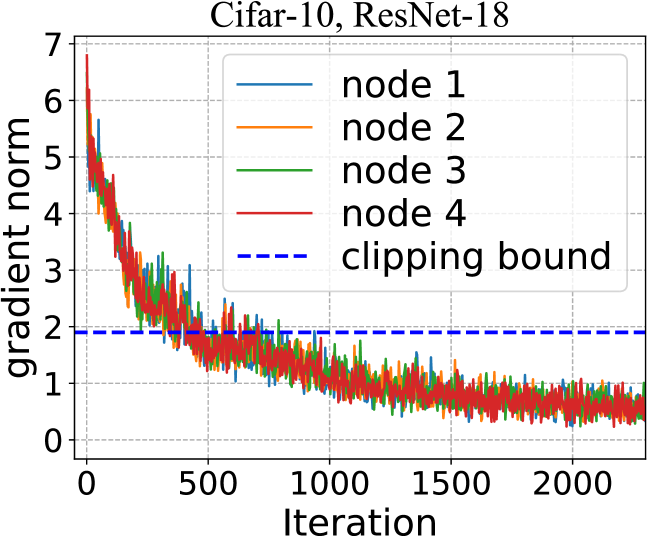
Figure 1: The evolution of the gradient norm when training ResNet-18 on Cifar-10 dataset in a fully decentralized setting with 4 nodes. It can be observed that the stochastic gradient norm at each node typically decays as training progresses, and eventually falls below the constant clipping bound (indicated by the blue dotted horizontal line) after certain number of iterations, which makes the clipping operation ineffective in the later stages of training.

To this end, we develop a new dynamic differentially private learning method for solving Problem (1) in fully decentralized settings, which enhances model accuracy while adhering to a total privacy budget constraint. The main contributions of this work are threefold:

• We propose a differentially private decentralized learning method with a dynamic DP Gaussian noise strategy (termed Dyn-D²P), tailored for general time-varying directed networks. In particular, each node adds noise with a variance calibrated by a dynamically decaying gradient clipping bound and an increasing per-step privacy budget appropriately allocated across iterations. This mechanism enables each node to apply dynamically decreasing noise, thereby enhancing model accuracy without compromising the total privacy budget.

• Theoretically, we investigate the impact of dynamic noise strategy on model utility for a general form of Dyn-D²P where clipping bounds and noise levels can be arbitrary sequences (c.f., Theorem 1), revealing the advantages of using dynamically decaying clipping bounds (c.f., Remark 1). By employing exponentially decaying sequences, we prove the utility bound of Dyn-D²P with explicit dependency on the network-related parameter, exhibiting a scaling factor of $1/\sqrt{n}$ in terms of the number of nodes up to a bias error term induced by gradient clipping (c.f., Corollary 1). To our knowledge, this is the first provable utility guarantee in the realm of dynamic differentially private decentralized learning.

• Extensive experiments are conducted to verify the performance of the proposed Dyn-D²P. The results show that, under the same total privacy budget, Dyn-D²P achieves superior accuracy compared to its counterpart using fixed-level DP Gaussian noise, especially under strong privacy guarantees. Moreover, we validate the robustness of Dyn-D²P against certain hyper-parameters related to the varying rates of gradient clipping bound and per-step privacy budget, and verify the performance of Dyn-D²P over different graphs and node numbers, which aligns with our theoretical findings.

2 Preliminary and Related Work

Differential privacy. Differential privacy was originally introduced in the seminal work by Dwork et al. Dwork et al. (2006) as a foundational concept for quantifying the privacy-preserving capabilities of randomized algorithms, and has now found widespread applications in a variety of domains that necessitate safeguarding against unintended information leakage Li et al. (2019a); Shin et al. (2018); Wei et al. (2021b). We recall the standard definition of DP as follows.

Definition 1 ($(\epsilon,\delta)$-DP Dwork et al. (2014)).

A randomized mechanism $\mathcal{M}$ with domain $\mathcal{D}$ and range $\mathcal{R}$ satisfies $(\epsilon,\delta)$-differential privacy (or $(\epsilon,\delta)$-DP), if for any two adjacent inputs $\mathrm{x},\mathrm{x}^{\prime}\in\mathcal{D}$ differing on a single entry and for any subset of outputs $O\subseteq\mathcal{R}$, it holds that

$$Pr\left[\mathcal{M}\left(\mathrm{x}\right)\in O\right]\leqslant e^{\epsilon}Pr\left[\mathcal{M}\left(\mathrm{x}^{\prime}\right)\in O\right]+\delta,$$ (2)

where the privacy budget $\epsilon$ denotes the privacy lower bound to measure a randomized query and $\delta$ is the probability of breaking this bound. Note that a smaller value of $\epsilon$ implies a stronger privacy guarantee.

The following proposition provides the Gaussian DP (GDP) mechanism to ensure privacy guarantee.

Proposition 1 ($\mu$-GDP Dong et al. (2019)).

Let $f:\mathcal{D}\rightarrow\mathbb{R}^{d}$ be a function and $S$ be its $l_{2}$ sensitivity. Then, drawing a random noise $N$ from Gaussian distribution with $N\thicksim\mathcal{N}\left(0,\sigma^{2}\mathbb{I}_{d}\right)$ and adding it to $f$ such that $\mathcal{M}(\mathrm{x})=f(\mathrm{x})+N$ satisfies $\mu$-GDP if $\sigma$ is set as

$$\sigma=S/\mu,$$ (3)

where $\mu$ is the privacy budget in the GDP framework, and a smaller value of $\mu$ implies a stronger privacy guarantee.

The above proposition shows that the variance $\sigma$ of the added noise required to ensure $\mu$-GDP is dependent on both privacy budget $\mu$ and sensitivity $S$. It should be noted that the above privacy guarantee in the sense of GDP can be transformed into the standard DP by the following proposition which shows that there is a one-to-one correspondence between $\epsilon$ and $\mu$ values when fixing $\delta$.

Proposition 2 (From $\mu$-GDP to $\left(\epsilon,\delta\right)$-DP Bu et al. (2020)).

A random mechanism is $\mu$-GDP if and only if it is $\left(\epsilon,\delta\right)$-DP for all $\epsilon\geqslant 0$, where

$$\delta=\Phi\left(-\frac{\epsilon}{\mu}+\frac{\mu}{2}\right)-e^{\epsilon}\Phi\left(-\frac{\epsilon}{\mu}-\frac{\mu}{2}\right),$$ (4)

and $\Phi\left(\cdot\right)$ is the Gaussian cumulative distribution function.

In what follows, we will review existing works related to achieving DP guarantees in machine learning and highlight the limitations in decentralized scenarios.

Decentralized learning methods with DP guarantee. DP guarantee is initially integrated into a centralized (single-node) setting for designing differentially private stochastic learning algorithms Abadi et al. (2016); Wang et al. (2017); Iyengar et al. (2019); Chen et al. (2020); Wang et al. (2020). Further, DP guarantee is considered in distributed learning with server-client structures and the representative works include McMahan et al. (2017b); Li et al. (2019b); Wang et al. (2019a); Wu et al. (2020); Wei et al. (2020); Zeng et al. (2021); Wei et al. (2021a); Li et al. (2022); Liu et al. (2022); Zhou et al. (2023); Wei et al. (2023). Recently, there have been efforts to achieve DP guarantees for fully decentralized learning algorithms. For example, Cheng et al. Cheng et al. (2018, 2019) achieve DP in fully decentralized learning for only strongly convex problems. Wang and Nedic Wang and Nedic (2024) achieve DP in fully decentralized architectures by tailoring gradient methods for deterministic optimization problems. For non-convex stochastic optimization problems as we consider in this work, Yu et al. Yu et al. (2021) present a differentially private decentralized learning method (DP²-SGD) based on D-PSGD Lian et al. (2017), which relies on a fixed communication topology and uses the basic composition theorem to bound the overall privacy loss. To have a tight privacy guarantee, Xu et al. Xu et al. (2022) propose a differentially private asynchronous decentralized learning method (A(DP)²SGD) based on AD-PSGD Lian et al. (2018), which provides privacy guarantee in the sense of Rényi differential privacy (RDP) Mironov (2017). However, it should be noted that the aforementioned two algorithms Yu et al. (2021); Xu et al. (2022) work only for undirected communication graphs which is often not satisfied in practical scenarios. Most recently, Li and Chi Li and Chi (2025) achieve DP guarantee as well as communication compression in decentralized learning for non-convex problems with the total privacy cost calculated via the moments accountant technique Abadi et al. (2016), while their methods are only applicable to time-invariant graphs.

Learning with dynamic DP Gaussian noise levels. For the aforementioned differentially private decentralized methods designed for non-convex stochastic optimization problems Yu et al. (2021); Xu et al. (2022); Li and Chi (2025), the injected fixed-level noise may exceed what is actually needed for privacy requirements as training progresses, especially during the later stages of training, since their estimated sensitivity based on constant/fixed gradient clipping bound $\bar{C}$ may not reflect the actual value of sensitivity (c.f., Figure 1). The overestimate of sensitivity may, indeed, lead to a waste of unnecessary privacy budget during the training process Wei et al. (2023). Therefore, a tighter sensitivity estimate is useful for improving model accuracy without sacrificing privacy. There have been few works dedicated to tightly estimate the sensitivity in a dynamic manner. For instance, a scheme of decaying gradient clipping bounds has been employed to estimate the sensitivity in differentially private centralized learning Du et al. (2021); Wei and Liu (2021), resulting in a decreasing amount of noise injection. In the realm of distributed learning, a similar strategy of dynamic clipping bounds is utilized in Andrew et al. (2021) to estimate sensitivity. Most recently, Wei et al. Wei et al. (2023) use the minimum of decaying clipping bounds and current gradient norms to estimate the $l_{2}$ sensitivity, leading to a less amount of noise injection. However, these distributed methods Andrew et al. (2021); Fu et al. (2022); Wei et al. (2023) only focus on server-client architecture and, most importantly, they do not provide any theoretical guarantee on model utility. In this paper, we aim to design a differentially private decentralized learning method that incorporates dynamic noise strategies in fully decentralized settings, and provide rigorous theoretical guarantee on model utility, as well as its utility-privacy trade-off.

3 Algorithm Development

In this section, we develop our differentially private decentralized learning methods using the Gaussian DP (GDP) framework as depicted in Proposition 1, which measures the privacy profile $\left(\epsilon,\delta\right)$ in terms of $\mu$ according to Proposition 2. We consider solving Problem (1) over the following general peer-to-peer network model.

Network model. The communication topology is modeled as a sequence of time-varying directed graph $\mathcal{G}^{k}=\left(\mathcal{V},\mathcal{E}^{k}\right)$, where $\mathcal{V}=\{1,2,...,n\}$ denotes the set of nodes and $\mathcal{E}^{k}\subset\mathcal{V}\times\mathcal{V}$ denotes the set of directed edges/links at iteration $k$. We associate each graph $\mathcal{G}^{k}$ with a non-negative mixing matrix $P^{k}\in\mathbb{R}^{n\times n}$ such that $(i,j)\in\mathcal{E}^{k}$ if $P_{i,j}^{k}>0$, i.e., node $i$ receiving a message from node $j$ at iteration $k$. We assume that each node is an in-neighbor of itself.

Algorithm 1 Dyn-D²P

1: Initialization: DP budget $(\epsilon,\delta)$, $x_{i}^{0}=z_{i}^{0}\in\mathbb{R}^{d}$, $w_{i}^{0}=1$, step size $\gamma>0$, total number of iterations $K$, initial clipping bound $C_{0}$ and hyper-parameters $\rho_{c}>1$ and $\rho_{\mu}>1$.

2: for $k=0,1,...,K-1$, at node $i$, do

3:  Randomly samples a local training data $\xi_{i}^{k}$ with the sampling probability $\frac{1}{J}$;

4:  Computes stochastic gradient at $z_{i}^{k}$: $\nabla f_{i}(z_{i}^{k};\xi_{i}^{k})$;

5:  Calculates the clipping bound by: $C_{k}=C_{0}\cdot\left(\rho_{c}\right)^{-\frac{k}{K}}$;

6:  Clips the stochastic gradient:

$$g_{i}^{k} =\mathrm{Clip}\left(\nabla f_{i}\left(z_{i}^{k};\xi_{i}^{k}\right);C_{k}\right)$$ (5)

$$=\nabla f_{i}\left(z_{i}^{k};\xi_{i}^{k}\right)\cdot\min\left\{1,\frac{C_{k}}{\left\|\nabla f_{i}\left(z_{i}^{k};\xi_{i}^{k}\right)\right\|}\right\};$$

7:  Calculates the per-step privacy budget by: $\mu_{k}=\mu_{0}\cdot\left(\rho_{\mu}\right)^{\frac{k}{K}}$ with $\mu_{0}$ the solution of (8);

8:  Calculates the DP noise variance by:

$$\sigma_{k}=\frac{C_{k}}{\mu_{k}}=\frac{C_{0}\cdot\left(\rho_{c}\right)^{-\frac{k}{K}}}{\mu_{0}\cdot\left(\rho_{\mu}\right)^{\frac{k}{K}}}=\frac{C_{0}}{\mu_{0}}\cdot\left(\rho_{c}\cdot\rho_{\mu}\right)^{-\frac{k}{K}};$$

9:  Draws randomized noise $N_{i}^{k}$ from the Gaussian distribution: $N_{i}^{k}\sim\mathcal{N}\left(0,\sigma_{k}^{2}\mathbb{I}_{d}\right);$

10:  Differentially private local SGD:

$$x_{i}^{k+\frac{1}{2}}=x_{i}^{k}-\gamma(g_{i}^{k}+N_{i}^{k});$$

11:  Sends $\left(x_{i}^{k+\frac{1}{2}},w_{i}^{k}\right)$ to all out-neighbors and receives $\left(x_{j}^{k+\frac{1}{2}},w_{j}^{k}\right)$ from all in-neighbors ;

12:  Updates $x_{i}^{k+1}$ by: $x_{i}^{k+1}=\sum_{j=1}^{n}{P_{i,j}^{k}x_{j}^{k+\frac{1}{2}}}$ ;

13:  Updates $w_{i}^{k+1}$ by: $w_{i}^{k+1}=\sum_{j=1}^{n}{P_{i,j}^{k}w_{j}^{k}}$;

14:  Updates $z_{i}^{k+1}$ by: $z_{i}^{k+1}=x_{i}^{k+1}/w_{i}^{k+1}$.

15: end for

The following assumptions are made on the mixing matrix and graph for the above network model to facilitate the subsequent utility analysis for our proposed algorithm.

Assumption 1 (Mixing matrix).

The non-negative mixing matrix $P^{k},\forall k$ is column-stochastic, i.e., $\mathbf{1}^{\top}P^{k}=\mathbf{1}^{\top}$, where $\mathbf{1}$ is an all-one vector.

Assumption 2 ($B$-strongly connected).

There exist positive integers $B$ and $\bigtriangleup$ such that the graph formed by the edge set $\bigcup\nolimits_{k=lB}^{\left(l+1\right)B-1}{\mathcal{E}^{k}}$ is strongly connected and has a diameter of at most $\bigtriangleup$ for $\forall l\geqslant 0$.

Now, we present our differentially private decentralized learning algorithm (termed Dyn-D²P) with a dynamic noise strategy, which works over the above general network model. The complete pseudocode is summarized in Algorithm 1. At a high level, Dyn-D²P is comprised of local SGD and the averaging of neighboring information, following a framework similar to SGP Assran et al. (2019) which employs the Push-Sum protocol Kempe et al. (2003) to tackle the unblanceness of directed graphs. However, the key distinction lies in the gradient clipping operation and the injection of DP Gaussian noise before performing local SGD. In particular, each node $i$ maintains three variables during the learning process: i) the model parameter $x_{i}^{k}$; ii) the scalar Push-Sum weight $w_{i}^{k}$ and iii) the de-biased parameter $z_{i}^{k}=x_{i}^{k}/w_{i}^{k}$, with the initialization of $x_{i}^{0}=z_{i}^{0}\in\mathbb{R}^{d}$ and $w_{i}^{0}=1$ for all nodes $i\in\mathcal{V}$. At each iteration $k$, each node $i$ updates as follows:

$$\texttt{Private local SGD:}\,\,\,x_{i}^{k+\frac{1}{2}}=x_{i}^{k}-\gamma\left(g_{i}^{k}+N_{i}^{k}\right),$$

$$\texttt{Averaging:}\,\,\,x_{i}^{k+1}=\sum_{j=1}^{n}{P_{i,j}^{k}x_{j}^{k+\frac{1}{2}}},w_{i}^{k+1}=\sum_{j=1}^{n}{P_{i,j}^{k}w_{j}^{k}},$$

$$\texttt{De-bias:}\,\,\,z_{i}^{k+1}=x_{i}^{k+1}/w_{i}^{k+1},$$

where $\gamma>0$ is the step size and $g_{i}^{k}$ is the clipped gradient (c.f., (5)). $N_{i}^{k}$ denotes the injected random noise to ensure $\mu_{k}$-GDP guarantee for node $i$ at iteration $k$. This noise is drawn from a Gaussian distribution with variance $\sigma_{k}^{2}$, calibrated according to the dynamic clipping bound $C_{k}$ and per-step privacy budget $\mu_{k}$. We note that the two key mechanisms in the proposed Dyn-D²P to achieve dynamic noise levels and enhance model accuracy include: i) dynamically decreasing clipping bounds (c.f., line 5 in Algorithm 1); ii) dynamically increasing per-step privacy budget (c.f., line 7 in Algorithm 1). The detailed design and motivation for these mechanisms will be explained as follows.

Dynamic decreasing clipping bounds. For differentially private decentralized learning algorithms, the gradient clipping operation is necessary for each node to bound the $l_{2}$ sensitivity of local SGD update and inject noise accordingly calibrated with $l_{2}$ sensitivity (i.e., clipping bound) and privacy budget. According to the previous discussion in Section 1 that the norm of stochastic gradient of each node typically decreases as training proceeds, we know that the stochastic gradient would not be clipped after some iteration $k$ if we use the constant clipping bound $\bar{C}$ as Yu et al. Yu et al. (2021); Xu et al. Xu et al. (2022); Li and Chi Li and Chi (2025) did, thus resulting in adding unnecessary excessive noise calibrated with $\bar{C}$ in the later stage of training. To address this issue, we employ a dynamic gradient clipping scheme for each node to reduce the clipping bounds $C_{k}$ across the updates. Compared to the fixed clipping bound $\bar{C}$ used in Yu et al. (2021); Xu et al. (2022); Li and Chi (2025), it can reduce the noise level after a particular $k$ when $C_{k}<\bar{C}$, which is beneficial for stabilizing the updates. In particular, we set the clipping bound $C_{k}$ as $C_{k}=C_{0}\cdot\left(\rho_{c}\right)^{-\frac{k}{K}}$, where $\rho_{c}>1$ is the hyper-parameter to control the decay rate of the clipping bound, $C_{0}$ is the initial clipping bound, and $K$ is the total number of iterations.

Dynamic increasing per-step privacy budget. Given a total privacy budget, the existing differentially private decentralized learning methods Yu et al. (2021); Xu et al. (2022); Li and Chi (2025) uniformly distribute privacy budgets across all training steps. However, recent works Zhu et al. (2019); Wei and Liu (2021); Wei et al. (2023) point out that it is relatively easier to leak privacy at the initial stage of the training process, and it becomes increasingly difficult as the training progresses. To this end, we allocate a small privacy budget in the early stages and gradually increase privacy budgets, i.e., setting $\mu_{k+1}\geqslant\mu_{k}$ for all $k\in\{0,1,2,...,K-1\}$. In addition, according to (3), we observe that small (resp. large) $\mu_{k}$ means adding large (resp. small) noise. Therefore, setting $\mu_{k+1}\geqslant\mu_{k}$ implies adding large (resp., small) noise in the early (resp., later) stages of decentralized training, which helps improve model accuracy. The intuition is that at the beginning of training, the model is far away from the optimum, and the gradient magnitudes are usually large (c.f., Figure 1); larger noise is thus allowed and even helps to quickly escape the saddle point Ge et al. (2015). As training proceeds, the model approaches the optimum and the gradient magnitude converge, smaller noise is then desired to stabilize the update for convergence.

The following proposition provides a way for privacy accounting of dynamic non-uniform $\mu_{k}$-GDP costs throughout the whole training process.

Proposition 3 (Composition theorem for GDP with varying $\mu_{k}$ Du et al. (2021)).

Consider a series of random mechanisms $M_{k}$ for $k\in\left\{0,1,2,...,K-1\right\}$, where $M_{k}$ is $\mu_{k}$-GDP, and each mechanism works only on a subsampled dataset by independent Bernoulli trial with probability $p$. After $K$ steps by composition of Gaussian mechanism, $M\triangleq M_{K-1}\otimes\cdot\cdot\cdot\otimes M_{1}\otimes M_{0}$ satisfies $\mu_{tot}$-GDP where

$$\mu_{tot}=p\cdot\sqrt{\sum_{k=0}^{K-1}{\left(e^{\mu_{k}^{2}}-1\right)}}.$$ (6)

To this end, we set the per-step privacy budget $\mu_{k}$ as

$$\mu_{k}=\mu_{0}\cdot\left(\rho_{\mu}\right)^{\frac{k}{K}},$$ (7)

where $\rho_{\mu}>1$ is the hyper-parameter controlling the growth rate of $\mu_{k}$, and $\mu_{0}$ is the initial privacy budget. Given the target total privacy budget $\left(\epsilon,\delta\right)$, the corresponding privacy budget in the GDP framework $\mu_{tot}$ can be obtained by (4). Substituting (7) into (6) with $p=\frac{1}{J}$, we have

$$J^{2}\mu_{tot}^{2}=\sum_{k=0}^{K-1}{\left(e^{\left(\mu_{0}\cdot\left(\rho_{\mu}\right)^{\frac{k}{K}}\right)^{2}}-1\right)},$$ (8)

and $\mu_{0}$ can be computed using a numerical method such as binary search. With a specific value of $\mu_{0}$ and $\rho_{\mu}$, the value of $\mu_{k}$ at each iteration $k$ can be calculated by (7).

In addition, we provide two by-product differentially private decentralized learning algorithms (termed Dyn[$C$]-D²P and Dyn[$\mu$]-D²P), which employ only dynamic clipping bound reduction method and dynamic per-step privacy budget growth method, respectively:

• Dyn[$C$]-D²P: we set the clipping bound $C_{k}$ as $C_{k}=C_{0}\cdot\left(\rho_{c}\right)^{-\frac{k}{K}}$ (c.f., Algorithm 1), while maintaining the per-step privacy budget $\mu_{k}$ the same for all iterations, i.e., fixing $\mu_{k}=\bar{\mu}$, $\forall k$. By substituting $\mu_{k}=\bar{\mu}$ into (6) in Proposition 3 with $p=\frac{1}{J}$, we obtain the closed-form solution of $\bar{\mu}$:

  $$\bar{\mu}=\sqrt{\log\left(\frac{J^{2}\mu_{tot}^{2}}{K}+1\right)}.$$ (9)

  With specific values of $C_{k}$ and $\bar{\mu}$, we can calibrate the DP noise variance at each iteration by $\sigma_{k}=\frac{C_{k}}{\bar{\mu}}=\frac{C_{0}}{\bar{\mu}}\cdot\left(\rho_{c}\right)^{-\frac{k}{K}}$. The complete pseudocode can be found in Algorithm 3 in the Appendix D.

• Dyn[$\mu$]-D²P: we set the per-step privacy budget $\mu_{k}$ as $\mu_{k}=\mu_{0}\cdot\left(\rho_{\mu}\right)^{\frac{k}{K}}$ (c.f., Algorithm 1), where $\mu_{0}$ is the solution of (8), while employing the fixed clipping bound, i.e., $C_{k}=\bar{C}$, $\forall k$. Therefore, the DP noise variance $\sigma_{k}$ at each iteration can be calculated by $\sigma_{k}=\frac{\bar{C}}{\mu_{k}}=\frac{\bar{C}}{\mu_{0}}\cdot\left(\rho_{\mu}\right)^{-\frac{k}{K}}$. The complete pseudocode can be found in Algorithm 4 in the Appendix D.

It can be observed that, given $\rho_{c}$ and $\rho_{\mu}$, the noise decay rate of Dyn-D²P is faster than that of Dyn[$C$]-D²P and Dyn[$\mu$]-D²P. We also present an algorithm termed Const-D²P as our baseline, which employs constant clipping bound (i.e., fixing $C_{k}=\bar{C}$, $\forall k$) and uniformly distributes privacy budgets across updates (i.e., $\mu_{k}=\bar{\mu}$, $\forall k$) as usually did in most of existing DP-based decentralized methods Yu et al. (2021); Xu et al. (2022); Li and Chi (2025). According to the values of $\bar{C}$ and $\bar{\mu}$ (c.f., (9)), the constant DP noise variance is $\bar{\sigma}=\frac{\bar{C}}{\bar{\mu}}$. The pseudocode of Const-D²P is summarized in Algorithm 5 in the Appendix D.

Algorithm 2 General Form of Dyn-D²P

1: Initialization: DP budget $(\epsilon,\delta)$, $x_{i}^{0}=z_{i}^{0}\in\mathbb{R}^{d}$, $w_{i}^{0}=1$, step size $\gamma>0$, total number of iterations $K$, clipping bounds $C_{0},...,C_{K-1}$, and noise levels $\tilde{\sigma}\cdot\tilde{\sigma}_{0},....,\tilde{\sigma}\cdot\tilde{\sigma}_{K-1}$.

2: for $k=0,1,...,K-1$, at node $i$, do

3:  Follows from line 3 and 4 in Algorithm 1;

4:  Gradient clipping: $g_{i}^{k}=\mathrm{Clip}\left(\nabla f_{i}\left(z_{i}^{k};\xi_{i}^{k}\right);C_{k}\right)$;

5:  Draws randomized noise $N_{i}^{k}$ from the Gaussian distribution: $N_{i}^{k}\sim\mathcal{N}\left(0,\tilde{\sigma}^{2}\mathbb{I}_{d}\right)$;

6:  Differentially private local SGD:

$$x_{i}^{k+\frac{1}{2}}=x_{i}^{k}-\gamma(g_{i}^{k}+\tilde{\sigma}_{k}N_{i}^{k});$$

7:  Follows from line 11-14 in Algorithm 1.

8: end for

4 Theoretical Analysis

In this section, we theoretically investigate the impact of our dynamic noise strategy on model utility guarantee and provide the utility bound for proposed Dyn-D²P given a certain privacy budget. We first present a general form of Dyn-D²P where $C_{k}$ and $\sigma_{k}$ can be arbitrarily predefined sequences (c.f., Algorithm 2). Different from Algorithm 1, we denote $\sigma_{k}=\tilde{\sigma}\cdot\tilde{\sigma}_{k}$ for convenience in subsequent analysis, and we term $\tilde{\sigma}$ as noise scale without loss of generality.

Then, we show that the DP guarantee for each node in Algorithm 2 can be achieved by setting the noise scale $\tilde{\sigma}$ properly according to the given total privacy budget $(\epsilon,\delta)$ as well as the equivalent privacy parameter $\mu_{tot}$, which is summarized in the following proposition.

Proposition 4 (Privacy guarantee).

Let $K$ be the total number of iterations. Algorithm 2 achieves $(\epsilon,\delta)$-DP guarantee for each node if we set the noise scale as

$$\tilde{\sigma}=\frac{1}{J\mu_{tot}}\sqrt{2\sum_{k=0}^{K-1}{\frac{C_{k}^{2}}{\tilde{\sigma}_{k}^{2}}}},$$ (10)

where $\mu_{tot}$ is the solution of (4) with $\mu=\mu_{tot}$.

Proof.

The complete proof can be found in the Appendix C. ∎

Next, we make the following commonly used assumption for the utility analysis of Algorithm 2.

Assumption 3 ($L$-smoothness).

For each function $f_{i},i\in\mathcal{V}$, there exists a constant $L>0$ such that $\left\|\nabla f_{i}\left(x\right)-\nabla f_{i}\left(y\right)\right\|\leqslant L\left\|x-y\right\|$.

Suppose Assumptions 1-3 hold, and assume that each per-sample gradient is upper-bounded, i.e., $\left\|\nabla f_{i}\left(z;\xi_{i}\right)\right\|\leqslant\varLambda$. Then, we are ready to provide the following theorem to characterize the utility guarantee of Algorithm 2.

Theorem 1 (Model utility).

If we set the noise scale $\tilde{\sigma}$ as in (10), Algorithm 2 can achieve $(\epsilon,\delta)$-DP guarantee for each node and has the following utility guarantee

$$\frac{1}{K}\sum_{k=0}^{K-1}{\mathbb{E}\left[\left\|\nabla f\left(\bar{x}^{k}\right)\right\|^{2}\right]}$$ (11)

$$\leqslant \frac{2\left(f\left(\bar{x}^{0}\right)-f^{*}\right)}{\gamma K}+\frac{3L^{2}\varPsi^{2}\sum_{i=1}^{n}{\left\|x_{i}^{0}\right\|^{2}}}{\left(1-q\right)^{2}nK}$$

$$+\frac{3\gamma^{2}L^{2}\varPsi^{2}}{\left(1-q\right)^{2}}\cdot\frac{1}{K}\sum_{k=0}^{K-1}{\cdot\frac{1}{n}\sum_{i=1}^{n}{\mathbb{E}\left[\left\|g_{i}^{k}\right\|^{2}\right]}}$$

$$+\gamma L\cdot\frac{1}{K}\sum_{k=0}^{K-1}{\mathbb{E}\left[\left\|\frac{1}{n}\sum_{i=1}^{n}{g_{i}^{k}}\right\|^{2}\right]}$$

$$+\left(\frac{6\gamma^{2}KL^{2}\varPsi^{2}d}{\left(1-q\right)^{2}J^{2}\mu_{tot}^{2}}+\frac{2\gamma KLd}{nJ^{2}\mu_{tot}^{2}}\right)\underset{\text{$\triangleq T_{1}$: privacy noise term}}{\underbrace{\frac{1}{K}\sum_{k=0}^{K-1}{\frac{C_{k}^{2}}{\tilde{\sigma}_{k}^{2}}}\frac{1}{K}\sum_{k=0}^{K-1}{\tilde{\sigma}_{k}^{2}}}},$$

$$+\underset{\text{$\triangleq T_{2}$: bias term}}{\underbrace{2\mathbb{E}\left[\frac{1}{K}\sum_{k=0}^{K-1}{\varLambda\left\|\nabla f\left(\bar{x}^{k}\right)\right\|\cdot\frac{1}{n}\sum_{i=1}^{n}{\mathcal{P}_{i}^{k}\left(C_{k}\right)}}\right]}}$$

where $\bar{x}^{k}=\frac{1}{n}\sum_{i=1}^{n}{x_{i}^{k}}$, $f^{*}=\underset{x\in\mathbb{R}^{d}}{\min}f\left(x\right)$ while $\varPsi$ and $q\in[0,1)$ are positive constants depending on the diameter of the network $\bigtriangleup$ and the sequence of mixing matrices $P^{k}$, whose definition can be found in Lemma 2 in the Appendix, $\mathcal{P}_{i}^{k}\left(C_{k}\right)$ denotes the probability of a stochastic gradient being clipped with clipping bound $C_{k}$ for node $i$ at iteration $k$.

Proof.

The complete proof can be found in the Appendix A. ∎

Remark 1 (On clipping bounds $C_{k}$).

The clipping of gradients will destroy the unbiased estimate of the local full gradient for each node, resulting in a constant bias error (reflected by $T_{2}$ in (11)). It is obvious that the smaller the clipping bound $C_{k}$, the greater the probability $\mathcal{P}_{i}^{k}\left(C_{k}\right)$ that clipping occurs at iteration $k$. Based on this fact, we know that in general, the bias term $T_{2}$ in (11) will be small if $C_{k}$’s are large and vise versa, given the same distribution of gradients. This implies that we can use large clipping bounds to reduce the bias term $T_{2}$. However, this may make the privacy noise error term $T_{1}$ in (11) become larger. It is thus essential to choose a proper sequence of $C_{k}$ that could effectively balance $T_{1}$ and $T_{2}$. However, finding an optimal sequence of clipping bounds to achieve the best trade-off necessitates knowledge of the distribution of the stochastic gradient, which is impossible to obtain in practice. The existing literature Andrew et al. (2021) points out that a noteworthy practical way is to keep the probability $\mathcal{P}_{i}^{k}\left(C_{i}^{k}\right)$ approximately constant. Considering that the norm of the gradient is decreasing as training progresses, $C_{k}$ should also be decreasing so as to keep $\mathcal{P}_{i}^{k}\left(C_{k}\right)$ roughly constant, which supports the design of our algorithm (c.f., Algorithm 1).

Next, we specify the sequences $C_{k}$ and $\tilde{\sigma}_{k}$ in Algorithm 2, yielding a special instance of dynamic clipping bound and noise scheduling as used in Algorithm 1. We then provide the corresponding utility bound in the following corollary.

Corollary 1.

Under the same conditions of Theorem 1, by setting $C_{k}=\Theta\left(\left(\rho_{c}\right)^{-\frac{k}{K}}\right)$ and $\tilde{\sigma}_{k}=\Theta\left(\left(\rho_{c}\cdot\rho_{\mu}\right)^{-\frac{k}{K}}\right)$ for some $\rho_{c}>1$ and $\rho_{\mu}>1$, if we set $\gamma=\frac{1}{\sqrt{n}J\mu_{tot}}$, $\gamma K=\sqrt{n}J\mu_{tot}$ and assume that $J\mu_{tot}>\sqrt{n}$, we have

$$\frac{1}{K}\sum_{k=0}^{K-1}{\mathbb{E}\left[\left\|\nabla f\left(\bar{x}^{k}\right)\right\|^{2}\right]}\leqslant\mathcal{O}\left(\frac{1}{\left(1-q\right)^{2}\sqrt{n}J\mu_{tot}}\right)+T_{2},$$ (12)

where $\mathcal{O}(\cdot)$ hides some constants, e.g., $L$, $\sum_{i=1}^{n}{\left\|x_{i}^{0}\right\|^{2}}$, $\varLambda$.

Proof.

The complete proof can be found in the Appendix B. ∎

Remark 2 (Tight utility bound).

Setting aside the non-vanishing bias term $T_{2}$, the utility bound derived in Corollary 1 exhibits explicit dependency on the network-related parameter $q$, and reveals a scaling factor of $1/\sqrt{n}$ with respect to the number of nodes $n$, which has never been observed in the previous differentially private decentralized algorithms Yu et al. (2021); Xu et al. (2022). By setting $n=1$ which corresponds to the centralized/single-node case, our utility result (12) can be reduced to $\mathcal{O}\left(1/J\mu_{tot}\right)$, sharing the same polynomial order as existing analysis Zhang et al. (2017); Du et al. (2021). To our best knowledge, we provide the first theoretical utility analysis for decentralized non-convex stochastic optimization with dynamic gradient clipping bounds and noise levels, highlighting the utility-privacy trade-off.

Remark 3 (Non-trivial analysis).

The exponential decay scheme of the sequences $C_{k}$ and $\tilde{\sigma}_{k}$ aligns with that of the sequences $C_{k}$ and $\sigma_{k}$ in Algorithm 1, up to a constant factor. Therefore, the theoretical result (utility bound) in Corollary 1 corroborates the parameter settings in Algorithm 1. We note that our analysis is non-trivial and can not be directly derived by extending the existing analysis Du et al. (2021) for the centralized/single-node case. The authors in Du et al. (2021) assume $C_{k}$ and $\tilde{\sigma}_{k}$ to be constant when deriving utility bounds, thereby simplifying the analysis (c.f., Theorem 1 in Du et al. (2021)). In contrast, our analysis involves a more precise setting of $C_{k}$ and $\tilde{\sigma}_{k}$ as outlined in Corollary 1, which requires a more sophisticated analysis (c.f., (35) to (36) in the Appendix for the derivation). We will also evaluate the impact of two hyper-parameters $\rho_{\mu}$ and $\rho_{c}$ on algorithm performance in the experimental section. The fixed schedule for the clipping bound and noise level in Corollary 1 is not the only option for our general algorithm form (Algorithm 2). Exploring alternative dynamic clipping bound mechanisms–such as using more complex schedules than exponential decaying method or adaptive clipping bound calculated based on the real-time gradient norm–would require additional heuristic efforts and complicate the theoretical utility analysis. We leave these explorations for future work.

5 Experiments

We conduct extensive experiments to verify the performance of proposed Dyn-D²P (c.f., Algorithm 1), with comparison to our two by-product algorithms Dyn[$C$]-D²P and Dyn[$\mu$]-D²P, and two baselines: i) Const-D²P, which employs fixed-level noise; ii) non-private decentralized learning algorithm, which does not use gradient clipping or add DP noise, and thus serves as the upper bound of model accuracy. All experiments are deployed in a server with Intel Xeon E5-2680 v4 CPU @ 2.40GHz and 8 Nvidia RTX 3090 GPUs, and are implemented with distributed communication package torch.distributed in PyTorch Paszke et al. (2017), where a process serves as a node, and inter-process communication is used to mimic communication among nodes.

Algorithm	$\boldsymbol{\epsilon=0.3}$	$\boldsymbol{\epsilon=0.7}$	$\boldsymbol{\epsilon=1}$	$\boldsymbol{\epsilon=3}$
Non-Private	82.16
Const-D2P	46.37	52.38	60.02	71.11
Dyn[$\mu$]-D2P	64.12	66.21	69.37	76.3
Dyn[$C$]-D2P	66.93	68.37	72.02	77.65
Dyn-D2P	71.87	72.14	75.06	79.89

Table 1: Final testing accuracy (%) for different algorithms when training ResNet-18 on Cifar-10 dataset, under different values of privacy budget $\epsilon$.

(a) Training loss

(b) Testing accuracy

Figure 2: Comparison of convergence performance for five algorithms under $(1,10^{-4})$-DP guarantee for each node, when training ResNet-18 on Cifar-10 dataset.

5.1 Experimental Setup

We compare five algorithms in a fully decentralized setting composed of 20 nodes, on two benchmark non-convex learning tasks: i) training ResNet-18 He et al. (2016) on Cifar-10 Krizhevsky (2009) dataset; ii) training shallow CNN model (composed of two convolution layers and two fully connected layers) on FashionMnist Xiao et al. (2017) dataset. We split shuffled datasets evenly to 20 nodes. For communication topology, unless otherwise stated, we use a time-varying directed exponential graph (refer to Appendix E for its definition). The learning rate is set to be $0.05$ for ResNet-18 training and $0.03$ for shallow CNN model training. Privacy parameters $\delta$ is set to be $10^{-4}$, and we test different values for $\epsilon$ which implies different levels of privacy guarantee. Other parameters such as $\bar{C}$, $C_{0}$, $\rho_{c}$ and $\rho_{\mu}$ are detailed in the Appendix F.1. Note that all experimental results are averaged over five repeated runs.

Algorithm	$\boldsymbol{\epsilon=0.3}$	$\boldsymbol{\epsilon=0.7}$	$\boldsymbol{\epsilon=1}$	$\boldsymbol{\epsilon=3}$
Non-Private	89.98
Const-D2P	45.37	58.63	74.65	80.81
Dyn[$\mu$]-D2P	81.12	82.98	82.23	84.36
Dyn[$C$]-D2P	82.93	83.65	84.06	84.98
Dyn-D2P	84.88	85.36	86.21	87.89

Table 2: Final testing accuracy (%) for different algorithms when training shallow CNN on FashionMnist dataset, under different values of privacy budget $\epsilon$.

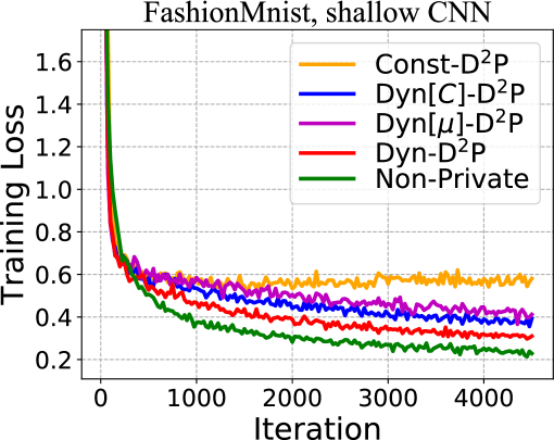
(a) Training loss

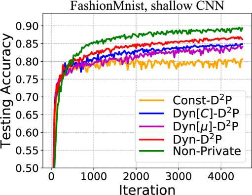
(b) Testing accuracy

Figure 3: Comparison of convergence performance for five algorithms under $(3,10^{-4})$-DP guarantee for each node, when training shallow CNN on FashionMnist dataset.

5.2 Superior Performance against Baseline Methods

For the ResNet-18 training task, we present the experimental result of final model accuracy in Table 1, and provide the plots of training loss/testing accuracy versus iteration in Figure 2 with a privacy budget of $\epsilon=1$ (the plots with other values of $\epsilon$ can be found in the Appendix G). It can be observed that our Dyn-D²P and two by-product algorithms (Dyn[$C$]-D²P and Dyn[$\mu$]-D²P) consistently outperform the baseline algorithm Const-D²P which employs constant noise. Among these above DP algorithms, Dyn-D²P achieves the highest model accuracy while maintaining the same level of privacy protection. Furthermore, a comparison of experimental results with different privacy budgets (i.e., varying values of $\epsilon$) shows that the stronger the level of required privacy protection (i.e., the smaller the value of budget $\epsilon$), the more pronounced the advantage in model accuracy with our dynamic noise strategy. In particular, when setting a small $\epsilon=0.3$ which implies a strong privacy guarantee, our Dyn-D²P achieves a $25\%$ higher model accuracy than Const-D²P employing constant noise strategies. These results verify the superiority of our dynamic noise approach.

For the shallow CNN training task, we present the experimental result of final model accuracy in Table 2, and provide the plots of training loss/testing accuracy in terms of iteration in Figure 3 with a privacy budget of $\epsilon=1$ (the plots with other values of $\epsilon$ can be found in the Appendix G). The takeaways from the experimental results are similar to previous experiments on the ResNet-18 training task, and our proposed Dyn-D²P performs much better than the baseline algorithm Const-D²P while maintaining the same level of privacy protection, which again highlights the superiority of our dynamic noise approach. In particular, under a strong level of required privacy guarantee with budget $\epsilon=0.3$, our Dyn-D²P achieves a $39\%$ higher model accuracy compared to Const-D²P.

5.3 Sensitivity to Hyper-parameters

In this part, we test the robustness of our algorithm (c.f., Algorithm 1) to different values of hyper-parameters $\rho_{c}$ and $\rho_{\mu}$. We use grid search to demonstrate the impact of these two parameters on the final model accuracy. It follows from the results as shown in Figure 4 that, our algorithm can almost maintain the final model accuracy and consistently improve model accuracy compared to Const-D²P across a wide range of $\rho_{c}$ and $\rho_{\mu}$, which implies that our proposed algorithm is robust to the value of hyper-parameter $\rho_{c}$ and $\rho_{\mu}$.

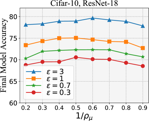
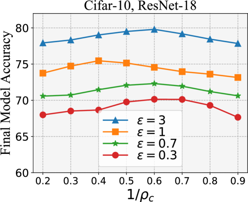
Figure 4: Illustration of the robustness of Dyn-D²P against the values of $\rho_{\mu}$ and $\rho_{c}$ under different privacy budget $\epsilon$.

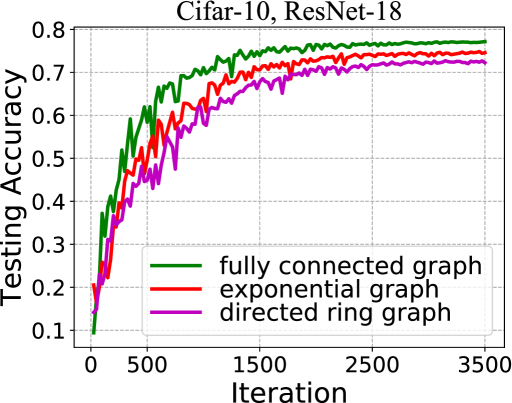
(a) $(1,10^{-4})$-DP guarantee

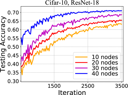
(b) $(1,10^{-4})$-DP guarantee

Figure 5: Comparison of convergence performance (model utility) for Dyn-D²P over (a) different graphs consisting of 20 nodes and (b) an exponential graph with different number of nodes, respectively.

5.4 Performance over Different Graphs and Node Numbers

First, we implement Dyn-D²P over a static directed ring graph, a time-varying directed exponential graph, and a fully connected graph, where the $q$ value w.r.t. these three graphs decreases in sequence. The experimental result shown in Figure 5(a) demonstrates that the model accuracy (utility) increases in sequence across these graphs. Then, we implement Dyn-D²P on a time-varying directed exponential graph consisting of different numbers of nodes (refer to Appendix F.2 for more details on the setup). It can be observed from Figure 5(b) that, increasing the number of nodes improves the model accuracy (utility). Note that both of these above observations align with the theoretical insights outlined in Corollary 1 and Remark 2.

6 Conclusion

In this work, we proposed a differentially private decentralized learning method Dyn-D²P, for non-convex optimization problems, which dynamically adjusts gradient clipping bounds and noise levels across the update. The proposed dynamic noise strategy allows us to enhance the model accuracy while maintaining the level of privacy guarantee. Extensive experiments show that our Dyn-D²P outperforms the existing counterparts with fixed-level noises, especially under strong privacy levels. Our analysis shows that the utility bound of Dyn-D²P exhibits an explicit dependency on the network-related parameter and enjoys a scaling factor of $1/\sqrt{n}$, up to a bias error term induced by gradient clipping. To our knowledge, we provide the first theoretical utility analysis for fully decentralized non-convex stochastic optimization with dynamic gradient clipping bounds and noise levels, highlighting the utility-privacy trade-off. We will focus on eliminating the bias term induced by gradient clipping in the future.

Appendix

Appendix A Proof of Theorem 1

To facilitate our analysis, we rewrite the update of Algorithm 2 in an equivalent compact form as follows:

$$X^{k+1}=\left(X^{k}-\gamma\left(G^{k}+\tilde{\sigma}_{k}N^{k}\right)\right)\left(P^{k}\right)^{\top}$$ (13)

where $\left(P^{k}\right)^{\top}\in\mathbb{R}^{n\times n}$ is the transpose of the mixing matrix $P^{k}$ at iteration $k$, and

$X^{k}:=\left[x_{1}^{k},x_{2}^{k},\cdot\cdot\cdot,x_{n}^{k}\right]\in\mathbb{R}^{d\times n}$: concatenation of all the nodes’ parameters at iteration $k$;

$Z^{k}:=\left[z_{1}^{k},z_{2}^{k},\cdot\cdot\cdot,z_{n}^{k}\right]\in\mathbb{R}^{d\times n}$: concatenation of all the nodes’ de-biased parameters at iteration $k$;

$\nabla F(Z^{k};\xi^{k}):=\left[\nabla f_{1}(z_{1}^{k};\xi_{1}^{k}),\nabla f_{2}(z_{2}^{k};\xi_{2}^{k}),...,\nabla f_{n}(z_{n}^{k};\xi_{n}^{k})\right]\in\mathbb{R}^{d\times n}$: concatenation of all the nodes’ stochastic gradients at iteration $k$;

$G^{k}:=\left[g_{1}^{k},g_{2}^{k},...,g_{n}^{k}\right]\in\mathbb{R}^{d\times n}$: concatenation of all the nodes’ clipped stochastic gradients at iteration $k$;

$N^{k}:=\left[N_{1}^{k},N_{2}^{k},...,N_{n}^{k}\right]\in\mathbb{R}^{d\times n}$: concatenation of all the nodes’ generated Gaussian noise at iteration $k$.

Now, let $\bar{x}^{k}=\frac{1}{n}X^{k}\mathbf{1}=\frac{1}{n}\sum_{i=1}^{n}{x_{i}^{k}}\in\mathbb{R}^{d}$ denote the average of all nodes’ parameters at iteration $k$. Then, the update of the average system of (13) becomes

$$\bar{x}^{k+1}=\bar{x}^{k}-\gamma\cdot\left(\frac{1}{n}\sum_{i=1}^{n}{g_{i}^{k}}+\tilde{\sigma}_{k}\cdot\frac{1}{n}\sum_{i=1}^{n}{N_{i}^{k}}\right),$$ (14)

which can be easily obtained by right multiplying $\frac{1}{n}\mathbf{1}$ from both sides of (13) and using the column-stochastic property of $P^{k}$ (c.f., Assumption 1). The above average system will be useful in subsequent analysis. In addition, we denote $\mathcal{F}^{k}:=\left\{\bigcup\nolimits_{i=1}^{n}{\left(x_{i}^{0},z_{i}^{0},\xi_{i}^{0},N_{i}^{0},\cdot\cdot\cdot,x_{i}^{k-1},z_{i}^{k-1},\xi_{i}^{k-1},N_{i}^{k-1},x_{i}^{k},z_{i}^{k}\right)}\right\}$ as the filtration of the history sequence up to iteration $k$, and define $\mathbb{E}_{k}\left[\cdot\right]=\mathbb{E}\left[\cdot\left|\mathcal{F}^{k}\right.\right]$ the conditional expectation given $\mathcal{F}^{k}$.

A.1 Bounding accumulative consensus error

We first provide two supporting lemmas to facilitate the subsequent analysis.

Lemma 1.

Let $\left\{v^{k}\right\}_{k=0}^{\infty}$ be a non-negative sequence and $\lambda\in(0,1)$. Then, we have

$$\left(\sum_{l=0}^{k}{\lambda^{k-l}v^{l}}\right)^{2}\leqslant\frac{1}{1-\lambda}\sum_{l=0}^{k}{\lambda^{k-l}\left(v^{l}\right)^{2}}.$$ (15)

Proof.

Using Cauchy-Swarchz inequality, we have

$$\left(\sum_{l=0}^{k}{\lambda^{k-l}v^{l}}\right)^{2} =\left(\sum_{l=0}^{k}{\lambda^{\frac{k-l}{2}}\left(\lambda^{\frac{k-l}{2}}v^{l}\right)}\right)^{2}$$

$$\leqslant\sum_{l=0}^{k}{\left(\lambda^{\frac{k-l}{2}}\right)^{2}}\cdot\sum_{l=0}^{k}{\left(\lambda^{\frac{k-l}{2}}v^{l}\right)^{2}}$$

$$\leqslant\frac{1}{1-\lambda}\sum_{l=0}^{k}{\lambda^{k-l}\left(v^{l}\right)^{2}},$$

which completes the proof. ∎

The following lemma bounds the distance between the de-biased parameters $z_{i}^{k}$ at each node $i$ and the node-wise average $\bar{x}^{k}$, which can be adapted from Lemma 3 in Assran et al. [2019].

Lemma 2.

Suppose that Assumptions 1 and 2 hold. Let $\varepsilon$ be the minimum of all non-zero mixing weights, $\lambda=1-n\varepsilon^{\bigtriangleup B}$ and $q=\lambda^{\frac{1}{\bigtriangleup B+1}}$. Then, there exists a constant

$$\varPsi<\frac{2\sqrt{d}\varepsilon^{-\bigtriangleup B}}{\lambda^{\frac{\bigtriangleup B+2}{\bigtriangleup B+1}}},$$ (16)

such that for any $i\in\mathcal{V}$ and $k\geqslant 0$, we have

$$\left\|z_{i}^{k}-\bar{x}^{k}\right\|\leqslant\varPsi q^{k}\left\|x_{i}^{0}\right\|+\gamma\varPsi\sum_{s=0}^{k}{q^{k-s}\left\|g_{i}^{s}+\tilde{\sigma}_{s}N_{i}^{s}\right\|}.$$ (17)

Now, we attempt to upper bound the accumulative consensus error $\sum_{k=0}^{K-1}{\frac{1}{n}\sum_{i=1}^{n}{\mathbb{E}\left[\left\|z_{i}^{k}-\bar{x}^{k}\right\|^{2}\right]}}$, which is summarized in the following lemma.

Lemma 3.

Suppose Assumptions 1 and 2 hold. Then, we have

$$\sum_{k=0}^{K-1}{\frac{1}{n}\sum_{i=1}^{n}{\mathbb{E}\left[\left\|z_{i}^{k}-\bar{x}^{k}\right\|^{2}\right]}}$$ (18)

$$\leqslant \frac{3\varPsi^{2}\sum_{i=1}^{n}{\left\|x_{i}^{0}\right\|^{2}}}{\left(1-q\right)^{2}n}+\frac{3\gamma^{2}\varPsi^{2}}{\left(1-q\right)^{2}}\sum_{k=0}^{K-1}{\cdot\frac{1}{n}\sum_{i=1}^{n}{\mathbb{E}\left[\left\|g_{i}^{k}\right\|^{2}\right]}}+\frac{3\gamma^{2}\varPsi^{2}d}{\left(1-q\right)^{2}}\sum_{k=0}^{K-1}{\tilde{\sigma}^{2}\tilde{\sigma}_{k}^{2}},$$

Proof.

According to (17), we have

$$\left\|z_{i}^{k}-\bar{x}^{k}\right\|\leqslant \varPsi q^{k}\left\|x_{i}^{0}\right\|+\gamma\varPsi\sum_{s=0}^{k}{q^{k-s}\left\|g_{i}^{s}\right\|}+\gamma\varPsi\sum_{s=0}^{k}{q^{k-s}\left\|\tilde{\sigma}_{s}N_{i}^{s}\right\|}$$ (19)

By squaring both sides of (19), we obtain

$$\left\|z_{i}^{k}-\bar{x}^{k}\right\|^{2}$$ (20)

$$\leqslant 3\varPsi^{2}q^{2k}\left\|x_{i}^{0}\right\|^{2}+3\gamma^{2}\varPsi^{2}\left(\sum_{s=0}^{k}{q^{k-s}\left\|g_{i}^{s}\right\|}\right)^{2}+3\gamma^{2}\varPsi^{2}\left(\sum_{s=0}^{k}{q^{k-s}\left\|\tilde{\sigma}_{s}N_{i}^{s}\right\|}\right)^{2}$$

$$\leqslant 3\varPsi^{2}q^{2k}\left\|x_{i}^{0}\right\|^{2}+\frac{3\gamma^{2}\varPsi^{2}}{1-q}\sum_{s=0}^{k}{q^{k-s}\left\|g_{i}^{s}\right\|^{2}}+\frac{3\gamma^{2}\varPsi^{2}}{1-q}\sum_{s=0}^{k}{q^{k-s}\left\|\tilde{\sigma}_{s}N_{i}^{s}\right\|^{2}},$$

where we used $\left\|a+b+c\right\|^{2}\leqslant 3\left\|a\right\|^{2}+3\left\|b\right\|^{2}+3\left\|c\right\|^{2}$ in the first inequality and Lemma 1 in the second, respectively.

Taking total expectation on both sides of (20) yields

$$\mathbb{E}\left[\left\|z_{i}^{k}-\bar{x}^{k}\right\|^{2}\right]$$ (21)

$$\leqslant 3\varPsi^{2}q^{2k}\left\|x_{i}^{0}\right\|^{2}+\frac{3\gamma^{2}\varPsi^{2}}{1-q}\sum_{s=0}^{k}{q^{k-s}\mathbb{E}\left[\left\|g_{i}^{s}\right\|^{2}\right]}+\frac{3\gamma^{2}\varPsi^{2}}{1-q}\sum_{s=0}^{k}{q^{k-s}\mathbb{E}\left[\left\|\tilde{\sigma}_{s}N_{i}^{s}\right\|^{2}\right]}$$

$$= 3\varPsi^{2}q^{2k}\left\|x_{i}^{0}\right\|^{2}+\frac{3\gamma^{2}\varPsi^{2}}{1-q}\sum_{s=0}^{k}{q^{k-s}\mathbb{E}\left[\left\|g_{i}^{s}\right\|^{2}\right]}+\frac{3\gamma^{2}\varPsi^{2}d}{1-q}\sum_{s=0}^{k}{q^{k-s}\cdot\tilde{\sigma}^{2}\tilde{\sigma}_{s}^{2}}.$$

Summing (21) from $i=1$ to $n$ and dividing by $n$, we have

$$\frac{1}{n}\sum_{i=1}^{n}{\mathbb{E}\left[\left\|z_{i}^{k}-\bar{x}^{k}\right\|^{2}\right]}$$ (22)

$$\leqslant \frac{3\varPsi^{2}q^{2k}}{n}\sum_{i=1}^{n}{\left\|x_{i}^{0}\right\|^{2}}+\frac{3\gamma^{2}\varPsi^{2}}{1-q}\sum_{s=0}^{k}{q^{k-s}\cdot\frac{1}{n}\sum_{i=1}^{n}{\mathbb{E}\left[\left\|g_{i}^{s}\right\|^{2}\right]}}+\frac{3\gamma^{2}\varPsi^{2}d}{1-q}\sum_{s=0}^{k}{q^{k-s}\cdot\tilde{\sigma}^{2}\tilde{\sigma}_{s}^{2}}.$$

Further, summing (22) from $k=0$ to $K-1$ leads to

$$\sum_{k=0}^{K-1}{\frac{1}{n}\sum_{i=1}^{n}{\mathbb{E}\left[\left\|z_{i}^{k}-\bar{x}^{k}\right\|^{2}\right]}}$$ (23)

$$\leqslant \frac{3\varPsi^{2}\sum_{i=1}^{n}{\left\|x_{i}^{0}\right\|^{2}}}{n}\cdot\sum_{k=0}^{K-1}{q^{2k}}+\frac{3\gamma^{2}\varPsi^{2}d}{1-q}\sum_{k=0}^{K-1}{\sum_{s=0}^{k}{q^{k-s}\cdot\tilde{\sigma}^{2}\tilde{\sigma}_{s}^{2}}}$$

$$+\frac{3\gamma^{2}\varPsi^{2}}{1-q}\sum_{k=0}^{K-1}{\sum_{s=0}^{k}{q^{k-s}\cdot\frac{1}{n}\sum_{i=1}^{n}{\mathbb{E}\left[\left\|g_{i}^{s}\right\|^{2}\right]}}}$$

$$\leqslant \frac{3\varPsi^{2}\sum_{i=1}^{n}{\left\|x_{i}^{0}\right\|^{2}}}{\left(1-q\right)^{2}n}+\frac{3\gamma^{2}\varPsi^{2}}{\left(1-q\right)^{2}}\sum_{k=0}^{K-1}{\cdot\frac{1}{n}\sum_{i=1}^{n}{\mathbb{E}\left[\left\|g_{i}^{k}\right\|^{2}\right]}}+\frac{3\gamma^{2}\varPsi^{2}d}{\left(1-q\right)^{2}}\sum_{k=0}^{K-1}{\tilde{\sigma}^{2}\tilde{\sigma}_{k}^{2}},$$

where in the last inequality we used the fact that $\sum_{k=0}^{K-1}{\sum_{s=0}^{k}{q^{k-s}a_{s}}}\leqslant\frac{1}{1-q}\sum_{k=0}^{K-1}{a_{k}}$. ∎

A.2 Proof of main result in Theorem 1

Applying the descent lemma to $f$ at $\bar{x}^{k}$ and $\bar{x}^{k+1}$, we have

$$f\left(\bar{x}^{k+1}\right)\leqslant f\left(\bar{x}^{k}\right)+\left<\nabla f\left(\bar{x}^{k}\right),\bar{x}^{k+1}-\bar{x}^{k}\right>+\frac{L}{2}\left\|\bar{x}^{k+1}-\bar{x}^{k}\right\|^{2}$$ (24)

$$\overset{\eqref{average_system}}{=} f\left(\bar{x}^{k}\right)-\gamma\left<\nabla f\left(\bar{x}^{k}\right),\frac{1}{n}\sum_{i=1}^{n}{g_{i}^{k}}+\tilde{\sigma}_{k}\cdot\frac{1}{n}\sum_{i=1}^{n}{N_{i}^{k}}\right>$$

$$+\frac{\gamma^{2}L}{2}\left\|\frac{1}{n}\sum_{i=1}^{n}{g_{i}^{k}}+\tilde{\sigma}_{k}\cdot\frac{1}{n}\sum_{i=1}^{n}{N_{i}^{k}}\right\|^{2}$$

$$= f\left(\bar{x}^{k}\right)-\gamma\left<\nabla f\left(\bar{x}^{k}\right),\frac{1}{n}\sum_{i=1}^{n}{g_{i}^{k}}+\tilde{\sigma}_{k}\cdot\frac{1}{n}\sum_{i=1}^{n}{N_{i}^{k}}\right>+\frac{\gamma^{2}L}{2}\left\|\frac{1}{n}\sum_{i=1}^{n}{g_{i}^{k}}\right\|^{2}$$

$$+\frac{\gamma^{2}L}{2}\tilde{\sigma}_{k}^{2}\left\|\frac{1}{n}\sum_{i=1}^{n}{N_{i}^{k}}\right\|^{2}+\gamma^{2}L\left<\frac{1}{n}\sum_{i=1}^{n}{g_{i}^{k}},\tilde{\sigma}_{k}\cdot\frac{1}{n}\sum_{i=1}^{n}{N_{i}^{k}}\right>.$$

Taking the expectation of both sides conditioned on $\mathcal{F}^{k}$ for the above inequality, we obtain

$$\mathbb{E}_{k}\left[f\left(\bar{x}^{k+1}\right)\right]\leqslant f\left(\bar{x}^{k}\right)-\gamma\left<\nabla f\left(\bar{x}^{k}\right),\frac{1}{n}\sum_{i=1}^{n}{\mathbb{E}_{k}\left[g_{i}^{k}\right]}\right>$$ (25)

$$+\frac{\gamma^{2}L}{2}\mathbb{E}_{k}\left[\left\|\frac{1}{n}\sum_{i=1}^{n}{g_{i}^{k}}\right\|^{2}\right]+\frac{\gamma^{2}L}{2}\tilde{\sigma}_{k}^{2}\mathbb{E}_{k}\left[\left\|\frac{1}{n}\sum_{i=1}^{n}{N_{i}^{k}}\right\|^{2}\right]$$

$$= f\left(\bar{x}^{k}\right)-\gamma\left<\nabla f\left(\bar{x}^{k}\right),\frac{1}{n}\sum_{i=1}^{n}{\mathbb{E}_{k}\left[g_{i}^{k}\right]}\right>$$

$$+\frac{\gamma^{2}L}{2}\mathbb{E}_{k}\left[\left\|\frac{1}{n}\sum_{i=1}^{n}{g_{i}^{k}}\right\|^{2}\right]+\frac{\gamma^{2}Ld}{2n}\tilde{\sigma}^{2}\tilde{\sigma}_{k}^{2}.$$

For the term of $\mathbb{E}_{k}\left[g_{i}^{k}\right]$, we have

$$\mathbb{E}_{k}\left[g_{i}^{k}\right]$$ (26)

$$= \mathbb{E}_{\xi_{i}^{k}}\left[\mathrm{Clip}\left(\nabla f_{i}\left(z_{i}^{k};\xi_{i}^{k}\right);C_{k}\right)\right]$$

$$\overset{\left(i\right)}{=} \sum_{j=1}^{J}{\frac{1}{J}\mathrm{Clip}\left(\nabla f_{i}\left(z_{i}^{k};j\right);C_{k}\right)}$$

$$\overset{\left(ii\right)}{=} \sum_{j=1}^{J}{\frac{1}{J}\mathbb{I}\left[\left\|\nabla f_{i}\left(z_{i}^{k};j\right)\right\|\leqslant C_{k}\right]\cdot\nabla f_{i}\left(z_{i}^{k};j\right)}+\sum_{j=1}^{J}{\frac{1}{J}\mathbb{I}\left[\left\|\nabla f_{i}\left(z_{i}^{k};j\right)\right\|>C_{k}\right]\cdot\frac{C_{k}\nabla f_{i}\left(z_{i}^{k};j\right)}{\left\|\nabla f_{i}\left(z_{i}^{k};j\right)\right\|}}$$

$$\overset{\left(iii\right)}{=} \frac{1}{J}\sum_{j=1}^{J}{\nabla f_{i}\left(z_{i}^{k};j\right)}+\sum_{j=1}^{J}{\left\{\frac{1}{J}\mathbb{I}\left[\left\|\nabla f_{i}\left(z_{i}^{k};j\right)\right\|>C_{k}\right]\cdot\nabla f_{i}\left(z_{i}^{k};j\right)\cdot\left(\frac{C_{k}}{\left\|\nabla f_{i}\left(z_{i}^{k};j\right)\right\|}-1\right)\right\}}$$

$$= \nabla f_{i}\left(z_{i}^{k}\right)+\sum_{j=1}^{J}{\left\{\frac{1}{J}\mathbb{I}\left[\left\|\nabla f_{i}\left(z_{i}^{k};j\right)\right\|>C_{k}\right]\cdot\nabla f_{i}\left(z_{i}^{k};j\right)\cdot\left(\frac{C_{k}}{\left\|\nabla f_{i}\left(z_{i}^{k};j\right)\right\|}-1\right)\right\}}.$$

where $\mathbb{I}\left[\cdot\right]$ is the indicator function; $(i)$ is based on the fact that each node uniformly at random chooses one out of $J$ data samples; $(ii)$ is due to the definition of gradient clipping operation; $(iii)$ is according to the fact of $\mathbb{I}\left[\left\|\nabla f_{i}\left(z_{i}^{k};j\right)\right\|\leqslant C_{k}\right]+\mathbb{I}\left[\left\|\nabla f_{i}\left(z_{i}^{k};j\right)\right\|>C_{k}\right]=1$.

Now, substituting (26) into (25), we have

$$\mathbb{E}_{k}\left[f\left(\bar{x}^{k+1}\right)\right]\leqslant f\left(\bar{x}^{k}\right)+A_{1}+A_{2}+\frac{\gamma^{2}L}{2}\mathbb{E}_{k}\left[\left\|\frac{1}{n}\sum_{i=1}^{n}{g_{i}^{k}}\right\|^{2}\right]+\frac{\gamma^{2}Ld}{2n}\tilde{\sigma}^{2}\tilde{\sigma}_{k}^{2}$$ (27)

with

$$A_{1}=-\gamma\left<\nabla f\left(\bar{x}^{k}\right),\frac{1}{n}\sum_{i=1}^{n}{\nabla f_{i}\left(z_{i}^{k}\right)}\right>$$

and

$$A_{2}=$$

$$-\gamma\left<\nabla f\left(\bar{x}^{k}\right),\frac{1}{n}\sum_{i=1}^{n}{\sum_{j=1}^{J}{\frac{1}{J}\mathbb{I}\left[\left\|\nabla f_{i}\left(z_{i}^{k};j\right)\right\|>C_{k}\right]\cdot}}\nabla f_{i}\left(z_{i}^{k};j\right)\cdot\left(\frac{C_{k}}{\left\|\nabla f_{i}\left(z_{i}^{k};j\right)\right\|}-1\right)\right>.$$

For $A_{1}$, we can bound it by

$$A_{1}= -\frac{\gamma}{2}\left\|\nabla f\left(\bar{x}^{k}\right)\right\|^{2}-\frac{\gamma}{2}\left\|\frac{1}{n}\sum_{i=1}^{n}{\nabla f_{i}\left(z_{i}^{k}\right)}\right\|^{2}+\frac{\gamma}{2}\left\|\frac{1}{n}\sum_{i=1}^{n}{\nabla f_{i}\left(z_{i}^{k}\right)}-\nabla f\left(\bar{x}^{k}\right)\right\|^{2}$$ (28)

$$\leqslant -\frac{\gamma}{2}\left\|\nabla f\left(\bar{x}^{k}\right)\right\|^{2}+\frac{\gamma}{2}\left\|\frac{1}{n}\sum_{i=1}^{n}{\left(\nabla f_{i}\left(z_{i}^{k}\right)-\nabla f_{i}\left(\bar{x}^{k}\right)\right)}\right\|^{2}$$

$$\leqslant -\frac{\gamma}{2}\left\|\nabla f\left(\bar{x}^{k}\right)\right\|^{2}+\frac{\gamma}{2n}\sum_{i=1}^{n}{\left\|\nabla f_{i}\left(z_{i}^{k}\right)-\nabla f_{i}\left(\bar{x}^{k}\right)\right\|^{2}}$$

$$\leqslant -\frac{\gamma}{2}\left\|\nabla f\left(\bar{x}^{k}\right)\right\|^{2}+\frac{\gamma L^{2}}{2n}\sum_{i=1}^{n}{\left\|z_{i}^{k}-\bar{x}^{k}\right\|^{2}},$$

where we have used Assumption 3 in the last inequality.

Using Cauchy-Schwartz inequality, we can bound $A_{2}$ by

$$A_{2}$$ (29)

$$\leqslant \gamma\left\|\nabla f\left(\bar{x}^{k}\right)\right\|\left\|\frac{1}{n}\sum_{i=1}^{n}{\sum_{j=1}^{J}{\frac{1}{J}\mathbb{I}\left[\left\|\nabla f_{i}\left(z_{i}^{k};j\right)\right\|>C_{k}\right]\cdot\nabla f_{i}\left(z_{i}^{k};j\right)\cdot\left(\frac{C_{k}}{\left\|\nabla f_{i}\left(z_{i}^{k};j\right)\right\|}-1\right)}}\right\|$$

$$\leqslant \gamma\left\|\nabla f\left(\bar{x}^{k}\right)\right\|\cdot\frac{1}{n}\sum_{i=1}^{n}{\sum_{j=1}^{J}{\frac{1}{J}\mathbb{I}\left[\left\|\nabla f_{i}\left(z_{i}^{k};j\right)\right\|>C_{k}\right]\cdot\varLambda}}$$

$$= \gamma\varLambda\left\|\nabla f\left(\bar{x}^{k}\right)\right\|\cdot\frac{1}{n}\sum_{i=1}^{n}{\mathcal{P}_{i}^{k}\left(C_{k}\right)},$$

where $\mathcal{P}_{i}^{k}\left(C_{k}\right)$ denotes the probability of a per-sample gradient being clipped with threshold $C_{k}$ for node $i$ at iteration $k$.

As a result, substituting (28) and (29) into (27), we further have

$$\mathbb{E}_{k}\left[f\left(\bar{x}^{k+1}\right)\right]\leqslant f\left(\bar{x}^{k}\right)-\frac{\gamma}{2}\left\|\nabla f\left(\bar{x}^{k}\right)\right\|^{2}+\frac{\gamma L^{2}}{2n}\sum_{i=1}^{n}{\left\|z_{i}^{k}-\bar{x}^{k}\right\|^{2}}$$ (30)

$$+\gamma\varLambda\left\|\nabla f\left(\bar{x}^{k}\right)\right\|\cdot\frac{1}{n}\sum_{i=1}^{n}{\mathcal{P}_{i}^{k}\left(C_{k}\right)}$$

$$+\frac{\gamma^{2}L}{2}\mathbb{E}_{k}\left[\left\|\frac{1}{n}\sum_{i=1}^{n}{g_{i}^{k}}\right\|^{2}\right]+\frac{\gamma^{2}Ld}{2n}\tilde{\sigma}^{2}\tilde{\sigma}_{k}^{2}.$$

Taking the total expectation on both sides of (30) yields

$$\mathbb{E}\left[f\left(\bar{x}^{k+1}\right)\right]\leqslant \mathbb{E}\left[f\left(\bar{x}^{k}\right)\right]-\frac{\gamma}{2}\mathbb{E}\left[\left\|\nabla f\left(\bar{x}^{k}\right)\right\|^{2}\right]$$ (31)

$$+\frac{\gamma L^{2}}{2n}\sum_{i=1}^{n}{\mathbb{E}\left[\left\|z_{i}^{k}-\bar{x}^{k}\right\|^{2}\right]}+\frac{\gamma^{2}L}{2}\mathbb{E}\left[\left\|\frac{1}{n}\sum_{i=1}^{n}{g_{i}^{k}}\right\|^{2}\right]$$

$$+\frac{\gamma^{2}Ld}{2n}\tilde{\sigma}^{2}\tilde{\sigma}_{k}^{2}+\gamma\mathbb{E}\left[\varLambda\left\|\nabla f\left(\bar{x}^{k}\right)\right\|\cdot\frac{1}{n}\sum_{i=1}^{n}{\mathcal{P}_{i}^{k}\left(C_{k}\right)}\right].$$

Summing the above inequality from $k=0$ to $K-1$, we obtain

$$\frac{\gamma}{2}\sum_{k=0}^{K-1}{\mathbb{E}\left[\left\|\nabla f\left(\bar{x}^{k}\right)\right\|^{2}\right]}\leqslant f\left(\bar{x}^{0}\right)-f^{*}+\frac{\gamma L^{2}}{2}\sum_{k=0}^{K-1}{\frac{1}{n}\sum_{i=1}^{n}{\mathbb{E}\left[\left\|z_{i}^{k}-\bar{x}^{k}\right\|^{2}\right]}}$$ (32)

$$+\frac{\gamma^{2}L}{2}\sum_{k=0}^{K-1}{\mathbb{E}\left[\left\|\frac{1}{n}\sum_{i=1}^{n}{g_{i}^{k}}\right\|^{2}\right]}+\frac{\gamma^{2}Ld}{2n}\tilde{\sigma}^{2}\sum_{k=0}^{K-1}{\tilde{\sigma}_{k}^{2}}$$

$$+\gamma\mathbb{E}\left[\sum_{k=0}^{K-1}{\varLambda\left\|\nabla f\left(\bar{x}^{k}\right)\right\|\cdot\frac{1}{n}\sum_{i=1}^{n}{\mathcal{P}_{i}^{k}\left(C_{k}\right)}}\right].$$

Substituting the upper bound of $\sum_{k=0}^{K-1}{\frac{1}{n}\sum_{i=1}^{n}{\mathbb{E}\left[\left\|z_{i}^{k}-\bar{x}^{k}\right\|^{2}\right]}}$ (c.f., (18) in Lemma 3) into (32), and multiplying $\frac{2}{\gamma K}$ on both sides, we obtain

$$\frac{1}{K}\sum_{k=0}^{K-1}{\mathbb{E}\left[\left\|\nabla f\left(\bar{x}^{k}\right)\right\|^{2}\right]}$$ (33)

$$\leqslant \frac{2\left(f\left(\bar{x}^{0}\right)-f^{*}\right)}{\gamma K}+\frac{3L^{2}\varPsi^{2}\sum_{i=1}^{n}{\left\|x_{i}^{0}\right\|^{2}}}{\left(1-q\right)^{2}nK}+\frac{3\gamma^{2}L^{2}\varPsi^{2}}{\left(1-q\right)^{2}}\cdot\frac{1}{K}\sum_{k=0}^{K-1}{\cdot\frac{1}{n}\sum_{i=1}^{n}{\mathbb{E}\left[\left\|g_{i}^{k}\right\|^{2}\right]}}$$

$$+\gamma L\cdot\frac{1}{K}\sum_{k=0}^{K-1}{\mathbb{E}\left[\left\|\frac{1}{n}\sum_{i=1}^{n}{g_{i}^{k}}\right\|^{2}\right]}+\underset{\text{$\triangleq T_{1}$: privacy noise term}}{\underbrace{\frac{3\gamma^{2}L^{2}\varPsi^{2}d}{\left(1-q\right)^{2}}\tilde{\sigma}^{2}\cdot\frac{1}{K}\sum_{k=0}^{K-1}{\tilde{\sigma}_{k}^{2}}+\frac{\gamma Ld}{n}\tilde{\sigma}^{2}\cdot\frac{1}{K}\sum_{k=0}^{K-1}{\tilde{\sigma}_{k}^{2}}}}$$

$$+\underset{\text{$\triangleq T_{2}$: bias term}}{\underbrace{2\mathbb{E}\left[\frac{1}{K}\sum_{k=0}^{K-1}{\varLambda\left\|\nabla f\left(\bar{x}^{k}\right)\right\|\cdot\frac{1}{n}\sum_{i=1}^{n}{P_{i}^{k}\left(C_{k}\right)}}\right]}}.$$

Substituting $\tilde{\sigma}=\frac{1}{J\mu_{tot}}\sqrt{2\sum_{k=0}^{K-1}{\frac{C_{k}^{2}}{\tilde{\sigma}_{k}^{2}}}}$ from Proposition 4 into the above (33), we can further obtain

$$\frac{1}{K}\sum_{k=0}^{K-1}{\mathbb{E}\left[\left\|\nabla f\left(\bar{x}^{k}\right)\right\|^{2}\right]}$$ (34)

$$\leqslant \frac{2\left(f\left(\bar{x}^{0}\right)-f^{*}\right)}{\gamma K}+\frac{3L^{2}\varPsi^{2}\sum_{i=1}^{n}{\left\|x_{i}^{0}\right\|^{2}}}{\left(1-q\right)^{2}nK}+\frac{3\gamma^{2}L^{2}\varPsi^{2}}{\left(1-q\right)^{2}}\cdot\frac{1}{K}\sum_{k=0}^{K-1}{\cdot\frac{1}{n}\sum_{i=1}^{n}{\mathbb{E}\left[\left\|g_{i}^{k}\right\|^{2}\right]}}$$

$$+\gamma L\cdot\frac{1}{K}\sum_{k=0}^{K-1}{\mathbb{E}\left[\left\|\frac{1}{n}\sum_{i=1}^{n}{g_{i}^{k}}\right\|^{2}\right]}+\left(\frac{6\gamma^{2}KL^{2}\varPsi^{2}d}{\left(1-q\right)^{2}J^{2}\mu_{tot}^{2}}+\frac{2\gamma KLd}{nJ^{2}\mu_{tot}^{2}}\right)\cdot\underset{\text{$\triangleq T_{1}$: privacy noise term}}{\underbrace{\frac{1}{K}\sum_{k=0}^{K-1}{\frac{C_{k}^{2}}{\tilde{\sigma}_{k}^{2}}}\cdot\frac{1}{K}\sum_{k=0}^{K-1}{\tilde{\sigma}_{k}^{2}}}}$$

$$+\underset{\text{$\triangleq T_{2}$: bias term}}{\underbrace{2\mathbb{E}\left[\frac{1}{K}\sum_{k=0}^{K-1}{\varLambda\left\|\nabla f\left(\bar{x}^{k}\right)\right\|\cdot\frac{1}{n}\sum_{i=1}^{n}{\mathcal{P}_{i}^{k}\left(C_{k}\right)}}\right]}},$$

which completes the proof of Theorem 1.

Appendix B Proof of Corollary 1

Proof.

Substituting $C_{k}=\Theta\left(\left(\rho_{c}\right)^{-\frac{k}{K}}\right)$ and $\tilde{\sigma}_{k}=\Theta\left(\left(\rho_{c}\cdot\rho_{\mu}\right)^{-\frac{k}{K}}\right)$ into $T_{1}$ in (34), we have

$$T_{1} =\Theta\left(\frac{1}{K}\sum_{k=0}^{K-1}{\frac{\left(\rho_{c}^{2}\right)^{-\frac{k}{K}}}{\left(\rho_{c}^{2}\cdot\rho_{\mu}^{2}\right)^{-\frac{k}{K}}}}\right)\cdot\Theta\left(\frac{1}{K}\sum_{k=0}^{K-1}{\left(\rho_{c}^{2}\cdot\rho_{\mu}^{2}\right)^{-\frac{k}{K}}}\right)$$ (35)

$$=\Theta\left(\frac{1}{K}\sum_{k=0}^{K-1}{\left(\rho_{\mu}^{2}\right)^{\frac{k}{K}}}\right)\cdot\Theta\left(\frac{1}{K}\sum_{k=0}^{K-1}{\left(\rho_{c}^{2}\cdot\rho_{\mu}^{2}\right)^{-\frac{k}{K}}}\right)$$

$$=\Theta\left(\frac{1}{K}\cdot\frac{\rho_{\mu}^{2}-1}{\left(\rho_{\mu}^{2}\right)^{\frac{1}{K}}-1}\right)\cdot\Theta\left(\frac{1}{K}\cdot\frac{1-\rho_{c}^{-2}\rho_{\mu}^{-2}}{1-\left(\rho_{c}^{-2}\rho_{\mu}^{-2}\right)^{\frac{1}{K}}}\right).$$

According to the fact that $\frac{1}{K}\cdot\frac{\rho_{\mu}^{2}-1}{\left(\rho_{\mu}^{2}\right)^{\frac{1}{K}}-1}<\frac{\rho_{\mu}^{2}-1}{\ln\left(\rho_{\mu}^{2}\right)}$ and $\frac{1}{K}\cdot\frac{1-\rho_{c}^{-2}\rho_{\mu}^{-2}}{1-\left(\rho_{c}^{-2}\rho_{\mu}^{-2}\right)^{\frac{1}{K}}}\leqslant 1$ for all $K\geqslant 1$, we have

$$T_{1}=\mathcal{O}\left(1\right).$$ (36)

Therefore, (34) becomes

$$\frac{1}{K}\sum_{k=0}^{K-1}{\mathbb{E}\left[\left\|\nabla f\left(\bar{x}^{k}\right)\right\|^{2}\right]}$$ (37)

$$\leqslant \mathcal{O}\left(\frac{1}{\gamma K}\right)+\frac{1}{\left(1-q\right)^{2}}\cdot\mathcal{O}\left(\frac{1}{K}\right)+\frac{1}{\left(1-q\right)^{2}}\cdot\mathcal{O}\left(\gamma^{2}\right)$$

$$+\mathcal{O}\left(\gamma\right)+\frac{1}{\left(1-q\right)^{2}}\cdot\mathcal{O}\left(\frac{\gamma^{2}K}{J^{2}\mu_{tot}^{2}}\right)+\mathcal{O}\left(\frac{\gamma K}{nJ^{2}\mu_{tot}^{2}}\right)+T_{2}.$$

Substituting $\gamma=\frac{1}{\sqrt{n}J\mu_{tot}}$ and $\gamma K=\sqrt{n}J\mu_{tot}$ into (37), and under our mild assumption of $J\mu_{tot}>\sqrt{n}$, we obtain

$$\frac{1}{K}\sum_{k=0}^{K-1}{\mathbb{E}\left[\left\|\nabla f\left(\bar{x}^{k}\right)\right\|^{2}\right]}\leqslant\mathcal{O}\left(\frac{1}{\left(1-q\right)^{2}\sqrt{n}J\mu_{tot}}\right)+T_{2},$$ (38)

which completes the proof of Corollary 1. ∎

Appendix C Proof of Proposition 4

Proof.

According to the definition of GDP in Proposition 1, we can easily know that each node satisfies $\mu_{k}$-GDP for each iteration in Algorithm 2, where

$$\mu_{k}=\frac{C_{k}}{\tilde{\sigma}\cdot\tilde{\sigma}_{k}}.$$

Further, based on (6), we can derive that each node satisfies $\hat{\mu}_{tot}$-GDP for overall training process, with

$$\hat{\mu}_{tot}=\frac{1}{J}\sqrt{\sum_{k=0}^{K-1}{\left(e^{\mu_{k}^{2}}-1\right)}}\overset{\left(a\right)}{<}\frac{1}{J}\sqrt{2\sum_{k=0}^{K-1}{\mu_{k}^{2}}}$$

where in $(a)$ we used the fact that $e^{x}-1<2x$ for $0\leqslant x\leqslant 1$. Given a privacy parameter $\mu_{tot}$ calculated according to $\left(\epsilon,\delta\right)$ based on (4), we use it to bound the above $\hat{\mu}_{tot}$, i.e.,

$$\hat{\mu}_{tot}<\frac{1}{J}\sqrt{2\sum_{k=0}^{K-1}{\mu_{k}^{2}}}=\frac{1}{J}\sqrt{2\sum_{k=0}^{K-1}{\frac{C_{k}^{2}}{\tilde{\sigma}^{2}\cdot\tilde{\sigma}_{k}^{2}}}}\leqslant\mu_{tot},$$

and we obtain

$$\tilde{\sigma}\geqslant\frac{1}{J\mu_{tot}}\sqrt{2\sum_{k=0}^{K-1}{\frac{C_{k}^{2}}{\tilde{\sigma}_{k}^{2}}}},$$

which is sufficient to guarantee each node in Algorithm 2 to satisfy $\mu_{tot}$-GDP as well as $\left(\epsilon,\delta\right)$-DP. ∎

Appendix D Missing Pseudocodes of Some Algorithms

In this section, we supplement the pseudocodes of Dyn[$C$]-D²P, Dyn[$\mu$]-D²P and Const-D²P we missed in the main text, which are given in Algorithm 3, Algorithm 4 and Algorithm 5, respectively.

Algorithm 3 Dyn[$C$]-D²P

1: Initialization: DP budget $(\epsilon,\delta)$, $x_{i}^{0}=z_{i}^{0}\in\mathbb{R}^{d}$, $w_{i}^{0}=1$, step size $\gamma>0$, total number of iterations $K$, initial clipping threshold $C_{0}$ and hyper-parameter $\rho_{c}$.

2: for $k=0,1,...,K-1$, at node $i$, do

3:  Randomly samples a local training data $\xi_{i}^{k}$ with the sampling probability $\frac{1}{J}$;

4:  Computes stochastic gradient at $z_{i}^{k}$: $\nabla f_{i}(z_{i}^{k};\xi_{i}^{k})$;

5:  Calculates the clipping bound by: $C_{k}=C_{0}\cdot\left(\rho_{c}\right)^{-\frac{k}{K}}$;

6:  Clips the stochastic gradient:

$$g_{i}^{k}=\mathrm{Clip}\left(\nabla f_{i}\left(z_{i}^{k};\xi_{i}^{k}\right);C_{k}\right)=\nabla f_{i}\left(z_{i}^{k};\xi_{i}^{k}\right)\cdot\min\left(1,\frac{C_{k}}{\left\|\nabla f_{i}\left(z_{i}^{k};\xi_{i}^{k}\right)\right\|}\right);$$

7:  Calculates the DP noise variance: $\sigma_{k}=\frac{C_{0}}{\bar{\mu}}\cdot\left(\rho_{c}\right)^{-\frac{k}{K}}$ ;

8:  Draws randomized noise $N_{i}^{k}$ from the Gaussian distribution: $N_{i}^{k}\sim\mathcal{N}\left(0,\sigma_{k}^{2}\mathbb{I}_{d}\right)$;

9:  Differentially private local SGD:

$$x_{i}^{k+\frac{1}{2}}=x_{i}^{k}-\gamma(g_{i}^{k}+N_{i}^{k});$$

10:  Sends $\left(x_{i}^{k+\frac{1}{2}},w_{i}^{k}\right)$ to all out-neighbors and receives $\left(x_{j}^{k+\frac{1}{2}},w_{j}^{k}\right)$ from all in-neighbors ;

11:  Updates $x_{i}^{k+1}$ by:  $x_{i}^{k+1}=\sum_{j=1}^{n}{P_{i,j}^{k}x_{j}^{k+\frac{1}{2}}}$ ;

12:  Updates $w_{i}^{k+1}$ by:  $w_{i}^{k+1}=\sum_{j=1}^{n}{P_{i,j}^{k}w_{j}^{k}}$ ;

13:  Updates $z_{i}^{k+1}$ by:  $z_{i}^{k+1}=x_{i}^{k+1}/w_{i}^{k+1}$ .

14: end for

Algorithm 4 Dyn[$\mu$]-D²P

1: Initialization: DP budget $(\epsilon,\delta)$, $x_{i}^{0}=z_{i}^{0}\in\mathbb{R}^{d}$, $w_{i}^{0}=1$, step size $\gamma>0$, total number of iterations $K$, fixed clipping threshold $\bar{C}$ and hyper-parameter $\rho_{\mu}$.

2: for $k=0,1,...,K-1$, at node $i$, do

3:  Randomly samples a local training data $\xi_{i}^{k}$ with the sampling probability $\frac{1}{J}$;

4:  Computes stochastic gradient at $z_{i}^{k}$: $\nabla f_{i}(z_{i}^{k};\xi_{i}^{k})$;

5:  Clips the stochastic gradient:

$$g_{i}^{k}=\mathrm{Clip}\left(\nabla f_{i}\left(z_{i}^{k};\xi_{i}^{k}\right);\bar{C}\right)=\nabla f_{i}\left(z_{i}^{k};\xi_{i}^{k}\right)\cdot\min\left\{1,\frac{\bar{C}}{\left\|\nabla f_{i}(z_{i}^{k};\xi_{i}^{k})\right\|}\right\};$$

6:  Calculates the DP noise variance: $\sigma_{k}=\frac{\bar{C}}{\mu_{0}}\cdot\left(\rho_{\mu}\right)^{-\frac{k}{K}}$ ;

7:  Draws randomized noise $N_{i}^{k}$ from the Gaussian distribution: $N_{i}^{k}\sim\mathcal{N}\left(0,\sigma_{k}^{2}\mathbb{I}_{d}\right)$ ;

8:  Differentially private local SGD:

$$x_{i}^{k+\frac{1}{2}}=x_{i}^{k}-\gamma(g_{i}^{k}+N_{i}^{k});$$

9:  Sends $\left(x_{i}^{k+\frac{1}{2}},w_{i}^{k}\right)$ to all out-neighbors and receives $\left(x_{j}^{k+\frac{1}{2}},w_{j}^{k}\right)$ from all in-neighbors ;

10:  Updates $x_{i}^{k+1}$ by:  $x_{i}^{k+1}=\sum_{j=1}^{n}{P_{i,j}^{k}x_{j}^{k+\frac{1}{2}}}$ ;

11:  Updates $w_{i}^{k+1}$ by:  $w_{i}^{k+1}=\sum_{j=1}^{n}{P_{i,j}^{k}w_{j}^{k}}$ ;

12:  Updates $z_{i}^{k+1}$ by:  $z_{i}^{k+1}=x_{i}^{k+1}/w_{i}^{k+1}$ .

13: end for

Algorithm 5 Const-D²P

1: Initialization: DP budget $(\epsilon,\delta)$, $x_{i}^{0}=z_{i}^{0}\in\mathbb{R}^{d}$, $w_{i}^{0}=1$, step size $\gamma>0$, total number of iterations $K$, and fixed clipping bound $\bar{C}$.

2: for $k=0,1,...,K-1$, at node $i$, do

3:  Randomly samples a local training data $\xi_{i}^{k}$ with the sampling probability $\frac{1}{J}$;

4:  Computes stochastic gradient at $z_{i}^{k}$: $\nabla f_{i}(z_{i}^{k};\xi_{i}^{k})$;

5:  Clips the stochastic gradient:

$$g_{i}^{k}=\mathrm{Clip}\left(\nabla f_{i}\left(z_{i}^{k};\xi_{i}^{k}\right);\bar{C}\right)=\nabla f_{i}\left(z_{i}^{k};\xi_{i}^{k}\right)\cdot\min\left\{1,\frac{\bar{C}}{\left\|\nabla f_{i}(z_{i}^{k};\xi_{i}^{k})\right\|}\right\};$$ (39)

6:  Draws randomized noise $N_{i}^{k}$ from the Gaussian distribution:

$$N_{i}^{k}\sim\mathcal{N}\left(0,\bar{\sigma}^{2}\mathbb{I}_{d}\right),$$

where $\bar{\sigma}=\frac{\bar{C}}{\bar{\mu}}$;

7:  Differentially private local SGD:

$$x_{i}^{k+\frac{1}{2}}=x_{i}^{k}-\gamma(g_{i}^{k}+N_{i}^{k});$$

8:  Sends $\left(x_{i}^{k+\frac{1}{2}},w_{i}^{k}\right)$ to all out-neighbors and receives $\left(x_{j}^{k+\frac{1}{2}},w_{j}^{k}\right)$ from all in-neighbors ;

9:  Updates $x_{i}^{k+1}$ by:  $x_{i}^{k+1}=\sum_{j=1}^{n}{P_{i,j}^{k}x_{j}^{k+\frac{1}{2}}}$ ;

10:  Updates $w_{i}^{k+1}$ by:  $w_{i}^{k+1}=\sum_{j=1}^{n}{P_{i,j}^{k}w_{j}^{k}}$ ;

11:  Updates $z_{i}^{k+1}$ by:  $z_{i}^{k+1}=x_{i}^{k+1}/w_{i}^{k+1}$ .

12: end for

Appendix E Missing Definition of Time-varying Directed Exponential Graph

We supplement the definition of time-varying directed exponential graph Assran et al. [2019] we missed in the main text. Specifically, $n$ nodes are ordered sequentially with their rank $0$,$1$…,$n-1$, and each node has out-neighbours that are $2^{0}$,$2^{1}$,…,$2^{\lfloor\log_{2}\left(n-1\right)\rfloor}$ hops away. Each node cycles through these out-neighbours, and only transmits messages to one of its out-neighbours at each iteration. For example, each node sends message to its $2^{0}$-hop out-neighbour at iteration $k$, and to its $2^{1}$-hop out-neighbour at iteration $k+1$, and so on. The above procedure will be repeated within the list of out-neighbours. Note that each node only sends and receives a single message at each iteration.

Appendix F Missing Experimental Setup

F.1 Hyper-parameter

We supplement the setup about the hyper-parameters we missed in the main text. Constant clipping bound $\bar{C}$, initial clipping bound $C_{0}$, $\rho_{c}$ and $\rho_{\mu}$ are given as follows:

• For Const-D²P (c.f., Algorithm 5), we test different value of constant clipping bound $\bar{C}$ from the set $\{5,4,3,2,1\}$ (resp. $\{2.5,2,1.5,1,0.5\}$) for ResNet-18 training (resp. shallow CNN model training), and choose the one with the best model performance for comparison with other algorithms;

• For Dyn[$C$]-D²P (c.f., Algorithm 3), we set the initial clipping bound $C_{0}$ to $7$ (resp. $4$) for ResNet-18 training (resp. shallow CNN model training), test different value of $\rho_{c}$ in the set $1/\rho_{c}\in\{0.1,0.2,0.3,0.4,0.5,0.6,0.7,0.8\}$ and choose the one with the best model performance for comparison with other algorithms;

• For Dyn[$\mu$]-D²P (c.f., Algorithm 4), we search the constant clipping bound $\bar{C}$ from the set $\{5,4,3,2,1\}$ (resp. $\{2.5,2,1.5,1,0.5\}$) for ResNet-18 training (resp. shallow CNN model training), test different value of $\rho_{\mu}$ in the set $1/\rho_{\mu}\in\{0.1,0.2,0.3,0.4,0.5,0.6,0.7,0.8\}$, and choose such a combination ($\bar{C}$ and $\rho_{\mu}$ ) that achieves the best model performance for comparison with other algorithms;

• For Dyn-D²P (c.f., Algorithm 1), we set the initial clipping bound $C_{0}$ to $7$ (resp. $4$) for ResNet-18 training (resp. shallow CNN model training), search $\rho_{c}$ and $\rho_{\mu}$ in the sets $1/\rho_{c},1/\rho_{\mu}\in\{0.1,0.2,0.3,0.4,0.5,0.6,0.7,0.8\}$ and choose the combination with the best model performance for comparison with other algorithms.

F.2 The number of training samples for each node

In this part, we supplement the experimental setup of experiments over different node numbers we missed in the main text. The 50,000 training images of the Cifar-10 dataset are evenly divided into 40 nodes, so each node has 1250 training images, i.e., the number of training samples $J=1250$. In the four experiments with different numbers of nodes, the number of training samples for each node was kept consistent.

Appendix G Missing Experimental Results

In this section, we supplement the experimental results we missed in the main text.

Figure 6-8 show the plots of training loss/testing accuracy versus iteration for different algorithms when training ResNet-18 on Cifar-10 dataset, under the different values of privacy budget $\epsilon$.

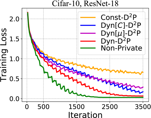
(a) $\epsilon=3,\delta=10^{-4}$

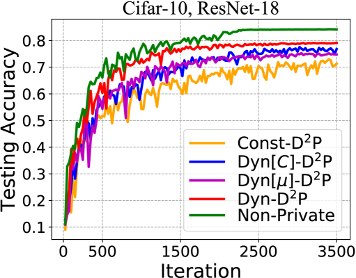
(b) $\epsilon=3,\delta=10^{-4}$

Figure 6: Comparison of convergence performance for five algorithms under $(3,10^{-4})$-DP guarantee for each node, when training ResNet-18 on Cifar-10 dataset.

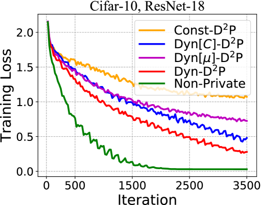
(a) $\epsilon=1,\delta=10^{-4}$

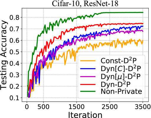
(b) $\epsilon=1,\delta=10^{-4}$

Figure 7: Comparison of convergence performance for five algorithms under $(1,10^{-4})$-DP guarantee for each node, when training ResNet-18 on Cifar-10 dataset.

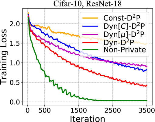
(a) $\epsilon=0.3,\delta=10^{-4}$

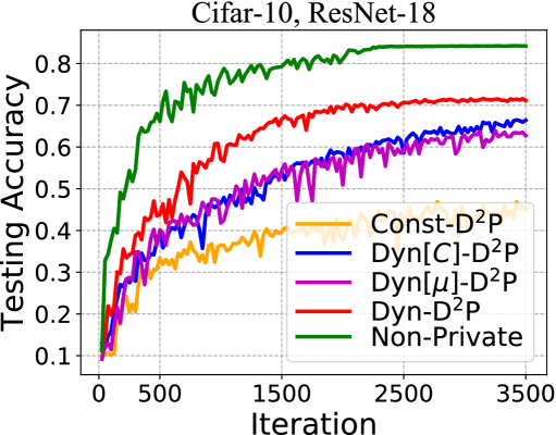
(b) $\epsilon=0.3,\delta=10^{-4}$

Figure 8: Comparison of convergence performance for five algorithms under $(0.3,10^{-4})$-DP guarantee for each node, when training ResNet-18 on Cifar-10 dataset.

For the experiments of training shallow CNN on FashionMnist dataset, we present the plots of training loss/testing accuracy versus iteration in Figure 9, 10 and 11, with the different values of privacy budget $\epsilon$. It can be observed that our Dyn-D²P and two by-product algorithms (Dyn[$C$]-D²P and Dyn[$\mu$]-D²P) consistently outperform the baseline algorithm Const-D²P which employs constant noise. Among these above DP algorithms, Dyn-D²P achieves the highest model accuracy while maintaining the same level of privacy protection. Furthermore, a comparison of experimental results with different privacy budgets (i.e., varying values of $\epsilon$) shows that the stronger the level of required privacy protection (i.e., the smaller the value of budget $\epsilon$), the more pronounced the advantage in model accuracy with our dynamic noise strategy. In particular, when setting a small $\epsilon=0.3$ which implies a strong privacy guarantee, our Dyn-D²P achieves a $39\%$ higher model accuracy than Const-D²P employing constant noise strategies. These results validate the superiority of our dynamic noise approach.

(a) Loss versus iteration

(b) Accuracy versus iteration

Figure 9: Comparison of convergence performance for five algorithms under $(3,10^{-4})$-DP guarantee for each node, when training shallow CNN on FashionMnist dataset.

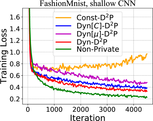
(a) $\epsilon=1,\delta=10^{-4}$

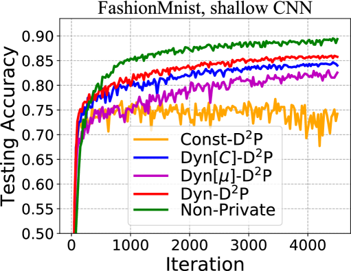
(b) $\epsilon=1,\delta=10^{-4}$

Figure 10: Comparison of convergence performance for five algorithms under $(1,10^{-4})$-DP guarantee for each node, when training shallow CNN on FashionMnist dataset.

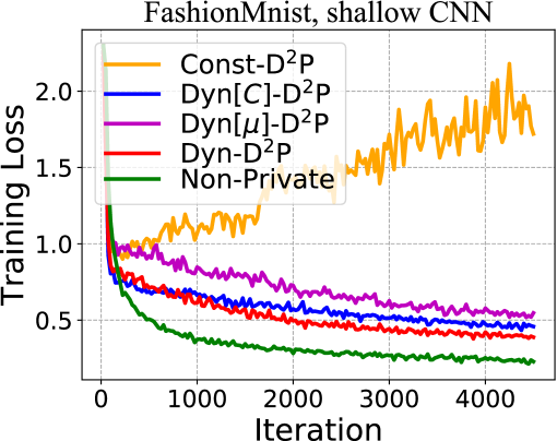
(a) $\epsilon=0.3,\delta=10^{-4}$

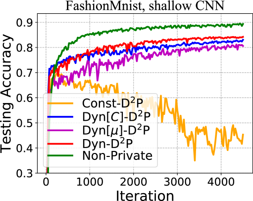
(b) $\epsilon=0.3,\delta=10^{-4}$

Figure 11: Comparison of convergence performance for five algorithms under $(0.3,10^{-4})$-DP guarantee for each node, when training shallow CNN on FashionMnist dataset.

References

- Abadi et al. [2016] Martin Abadi, Andy Chu, Ian Goodfellow, H Brendan McMahan, Ilya Mironov, Kunal Talwar, and Li Zhang. Deep learning with differential privacy. In Proceedings of the 2016 ACM SIGSAC conference on computer and communications security, pages 308–318, 2016.
- Andrew et al. [2021] Galen Andrew, Om Thakkar, Brendan McMahan, and Swaroop Ramaswamy. Differentially private learning with adaptive clipping. Advances in Neural Information Processing Systems, 34:17455–17466, 2021.
- Assran et al. [2019] Mahmoud Assran, Nicolas Loizou, Nicolas Ballas, and Mike Rabbat. Stochastic gradient push for distributed deep learning. In International Conference on Machine Learning, pages 344–353. PMLR, 2019.
- Bu et al. [2020] Zhiqi Bu, Jinshuo Dong, Qi Long, and Weijie J Su. Deep learning with gaussian differential privacy. arXiv preprint arXiv:1911.11607, 2020.
- Chen et al. [2020] Xiangyi Chen, Steven Z Wu, and Mingyi Hong. Understanding gradient clipping in private sgd: A geometric perspective. Advances in Neural Information Processing Systems, 33:13773–13782, 2020.
- Cheng et al. [2018] Hsin-Pai Cheng, Patrick Yu, Haojing Hu, Feng Yan, Shiyu Li, Hai Li, and Yiran Chen. LEASGD: an efficient and privacy-preserving decentralized algorithm for distributed learning. arXiv preprint arXiv:1811.11124, 2018.
- Cheng et al. [2019] Hsin-Pai Cheng, Patrick Yu, Haojing Hu, Syed Zawad, Feng Yan, Shiyu Li, Hai Li, and Yiran Chen. Towards decentralized deep learning with differential privacy. In International Conference on Cloud Computing, pages 130–145. Springer, 2019.
- Dong et al. [2019] Jinshuo Dong, Aaron Roth, and Weijie J Su. Gaussian differential privacy. arXiv preprint arXiv:1905.02383, 2019.
- Du et al. [2021] Jian Du, Song Li, Xiangyi Chen, Siheng Chen, and Mingyi Hong. Dynamic differential-privacy preserving sgd. In International Conference on Machine Learning. PMLR, 2021.
- Dwork et al. [2006] Cynthia Dwork, Krishnaram Kenthapadi, Frank McSherry, Ilya Mironov, and Moni Naor. Our data, ourselves: Privacy via distributed noise generation. In Annual international conference on the theory and applications of cryptographic techniques, pages 486–503. Springer, 2006.
- Dwork et al. [2014] Cynthia Dwork, Aaron Roth, et al. The algorithmic foundations of differential privacy. Foundations and Trends® in Theoretical Computer Science, 9(3–4):211–407, 2014.
- Fu et al. [2022] Jie Fu, Zhili Chen, and Xiao Han. Adap DP-FL: Differentially private federated learning with adaptive noise. In 2022 IEEE International Conference on Trust, Security and Privacy in Computing and Communications (TrustCom), pages 656–663. IEEE, 2022.
- Ge et al. [2015] Rong Ge, Furong Huang, Chi Jin, and Yang Yuan. Escaping from saddle points—online stochastic gradient for tensor decomposition. In Conference on Learning Theory, pages 797–842. PMLR, 2015.
- He et al. [2016] Kaiming He, Xiangyu Zhang, Shaoqing Ren, and Jian Sun. Deep residual learning for image recognition. In Proceedings of the IEEE conference on computer vision and pattern recognition, pages 770–778, 2016.
- Iyengar et al. [2019] Roger Iyengar, Joseph P Near, Dawn Song, Om Thakkar, Abhradeep Thakurta, and Lun Wang. Towards practical differentially private convex optimization. In 2019 IEEE Symposium on Security and Privacy (SP), pages 299–316. IEEE, 2019.
- Kempe et al. [2003] David Kempe, Alin Dobra, and Johannes Gehrke. Gossip-based computation of aggregate information. In 44th Annual IEEE Symposium on Foundations of Computer Science, 2003. Proceedings., pages 482–491. IEEE, 2003.
- Koloskova et al. [2019] Anastasiia Koloskova, Tao Lin, Sebastian Urban Stich, and Martin Jaggi. Decentralized deep learning with arbitrary communication compression. In Proceedings of the 8th International Conference on Learning Representations, 2019.
- Krizhevsky [2009] Alex Krizhevsky. Learning multiple layers of features from tiny images. Master’s thesis, University of Toronto, 2009.
- Langer et al. [2020] Matthias Langer, Zhen He, Wenny Rahayu, and Yanbo Xue. Distributed training of deep learning models: A taxonomic perspective. IEEE Transactions on Parallel and Distributed Systems, 31(12):2802–2818, 2020.
- Li and Chi [2025] Boyue Li and Yuejie Chi. Convergence and privacy of decentralized nonconvex optimization with gradient clipping and communication compression. IEEE Journal of Selected Topics in Signal Processing, 2025.
- Li et al. [2019a] Jeffrey Li, Mikhail Khodak, Sebastian Caldas, and Ameet Talwalkar. Differentially private meta-learning. arXiv preprint arXiv:1909.05830, 2019.
- Li et al. [2019b] Yanan Li, Shusen Yang, Xuebin Ren, and Cong Zhao. Asynchronous federated learning with differential privacy for edge intelligence. arXiv preprint arXiv:1912.07902, 2019.
- Li et al. [2022] Zhize Li, Haoyu Zhao, Boyue Li, and Yuejie Chi. SoteriaFL: A unified framework for private federated learning with communication compression. Advances in Neural Information Processing Systems, 35:4285–4300, 2022.
- Lian et al. [2017] Xiangru Lian, Ce Zhang, Huan Zhang, Cho-Jui Hsieh, Wei Zhang, and Ji Liu. Can decentralized algorithms outperform centralized algorithms? a case study for decentralized parallel stochastic gradient descent. Advances in Neural Information Processing Systems, 30, 2017.
- Lian et al. [2018] Xiangru Lian, Wei Zhang, Ce Zhang, and Ji Liu. Asynchronous decentralized parallel stochastic gradient descent. In International Conference on Machine Learning, pages 3043–3052. PMLR, 2018.
- Liu et al. [2022] Tianyu Liu, Boya Di, Bin Wang, and Lingyang Song. Loss-privacy tradeoff in federated edge learning. IEEE Journal of Selected Topics in Signal Processing, 16(3):546–558, 2022.
- McMahan et al. [2017a] Brendan McMahan, Eider Moore, Daniel Ramage, Seth Hampson, and Blaise Aguera y Arcas. Communication-efficient learning of deep networks from decentralized data. In Artificial intelligence and statistics, pages 1273–1282. PMLR, 2017.
- McMahan et al. [2017b] H Brendan McMahan, Daniel Ramage, Kunal Talwar, and Li Zhang. Learning differentially private recurrent language models. arXiv preprint arXiv:1710.06963, 2017.
- Mironov [2017] Ilya Mironov. Rényi differential privacy. In 2017 IEEE 30th computer security foundations symposium (CSF), pages 263–275. IEEE, 2017.
- Paszke et al. [2017] Adam Paszke, Sam Gross, Soumith Chintala, and Gregory Chanan. Pytorch: Tensors and dynamic neural networks in python with strong gpu acceleration. PyTorch: Tensors and dynamic neural networks in Python with strong GPU acceleration, 6(3):67, 2017.
- Shin et al. [2018] Hyejin Shin, Sungwook Kim, Junbum Shin, and Xiaokui Xiao. Privacy enhanced matrix factorization for recommendation with local differential privacy. IEEE Transactions on Knowledge and Data Engineering, 30(9):1770–1782, 2018.
- Tang et al. [2018] Hanlin Tang, Xiangru Lian, Ming Yan, Ce Zhang, and Ji Liu. : Decentralized training over decentralized data. In International Conference on Machine Learning, pages 4848–4856. PMLR, 2018.
- Wang and Nedic [2024] Yongqiang Wang and Angelia Nedic. Tailoring gradient methods for differentially private distributed optimization. IEEE Transactions on Automatic Control, 69(2):872–887, 2024.
- Wang et al. [2017] Di Wang, Minwei Ye, and Jinhui Xu. Differentially private empirical risk minimization revisited: Faster and more general. Advances in Neural Information Processing Systems, 30, 2017.
- Wang et al. [2019a] Lingxiao Wang, Bargav Jayaraman, David Evans, and Quanquan Gu. Efficient privacy-preserving stochastic nonconvex optimization. arXiv e-prints, pages arXiv–1910, 2019.
- Wang et al. [2019b] Zhibo Wang, Mengkai Song, Zhifei Zhang, Yang Song, Qian Wang, and Hairong Qi. Beyond inferring class representatives: User-level privacy leakage from federated learning. In IEEE INFOCOM 2019-IEEE conference on computer communications, pages 2512–2520. IEEE, 2019.
- Wang et al. [2020] Di Wang, Hanshen Xiao, Srinivas Devadas, and Jinhui Xu. On differentially private stochastic convex optimization with heavy-tailed data. In International Conference on Machine Learning, pages 10081–10091. PMLR, 2020.
- Wei and Liu [2021] Wenqi Wei and Ling Liu. Gradient leakage attack resilient deep learning. IEEE Transactions on Information Forensics and Security, 17:303–316, 2021.
- Wei et al. [2020] Kang Wei, Jun Li, Ming Ding, Chuan Ma, Howard H Yang, Farhad Farokhi, Shi Jin, Tony QS Quek, and H Vincent Poor. Federated learning with differential privacy: Algorithms and performance analysis. IEEE Transactions on Information Forensics and Security, 15:3454–3469, 2020.
- Wei et al. [2021a] Kang Wei, Jun Li, Ming Ding, Chuan Ma, Hang Su, Bo Zhang, and H Vincent Poor. User-level privacy-preserving federated learning: Analysis and performance optimization. IEEE Transactions on Mobile Computing, 21(9):3388–3401, 2021.
- Wei et al. [2021b] Kang Wei, Jun Li, Chuan Ma, Ming Ding, Cailian Chen, Shi Jin, Zhu Han, and H Vincent Poor. Low-latency federated learning over wireless channels with differential privacy. IEEE Journal on Selected Areas in Communications, 40(1):290–307, 2021.
- Wei et al. [2023] Wenqi Wei, Ling Liu, Jingya Zhou, Ka-Ho Chow, and Yanzhao Wu. Securing distributed sgd against gradient leakage threats. IEEE Transactions on Parallel and Distributed Systems, 2023.
- Wu et al. [2020] Nan Wu, Farhad Farokhi, David Smith, and Mohamed Ali Kaafar. The value of collaboration in convex machine learning with differential privacy. In 2020 IEEE Symposium on Security and Privacy (SP), pages 304–317. IEEE, 2020.
- Xiao et al. [2017] Han Xiao, Kashif Rasul, and Roland Vollgraf. Fashion-mnist: a novel image dataset for benchmarking machine learning algorithms. arXiv preprint arXiv:1708.07747, 2017.
- Xu et al. [2022] Jie Xu, Wei Zhang, and Fei Wang. A(DP)ˆ2SGD: Asynchronous decentralized parallel stochastic gradient descent with differential privacy. IEEE Transactions on Pattern Analysis and Machine Intelligence, 44(11):8036–8047, 2022.
- Yu et al. [2021] Dongxiao Yu, Zongrui Zou, Shuzhen Chen, Youming Tao, Bing Tian, Weifeng Lv, and Xiuzhen Cheng. Decentralized parallel sgd with privacy preservation in vehicular networks. IEEE Transactions on Vehicular Technology, 70(6):5211–5220, 2021.
- Zeng et al. [2021] Yiming Zeng, Yixuan Lin, Yuanyuan Yang, and Ji Liu. Differentially private federated temporal difference learning. IEEE Transactions on Parallel and Distributed Systems, 33(11):2714–2726, 2021.
- Zhang et al. [2017] Jiaqi Zhang, Kai Zheng, Wenlong Mou, and Liwei Wang. Efficient private erm for smooth objectives. In Proceedings of the 26th International Joint Conference on Artificial Intelligence, pages 3922–3928, 2017.
- Zhou et al. [2023] Yipeng Zhou, Xuezheng Liu, Yao Fu, Di Wu, Jessie Hui Wang, and Shui Yu. Optimizing the numbers of queries and replies in convex federated learning with differential privacy. IEEE Transactions on Dependable and Secure Computing, 2023.
- Zhu et al. [2019] Ligeng Zhu, Zhijian Liu, and Song Han. Deep leakage from gradients. Advances in neural information processing systems, 32, 2019.
- Zhu et al. [2024] Zehan Zhu, Ye Tian, Yan Huang, Jinming Xu, and Shibo He. R-FAST: Robust fully-asynchronous stochastic gradient tracking over general topology. IEEE Transactions on Signal and Information Processing over Networks, 10:665–678, 2024.
- Zinkevich et al. [2010] Martin Zinkevich, Markus Weimer, Lihong Li, and Alex Smola. Parallelized stochastic gradient descent. Advances in neural information processing systems, 23, 2010.