N-body simulations of the Self–Confinement of Viscous Self–Gravitating Narrow Eccentric Planetary Ringlets

Abstract

Narrow eccentric planetary ringlets have sharp edges, sizable eccentricity gradients, and a confinement mechanism that prevents radial spreading due to ring viscosity. Most proposed ringlet confinement mechanisms presume that there are one or more shepherd satellites whose gravitational perturbations keeps the ringlet confined radially, but the absence of such shepherds in Cassini observations of Saturn’s rings casts doubt upon those ringlet confinement mechanisms. The following uses a suite of N-body simulations to explore an alternate scenario, whereby ringlet self-gravity drives a narrow eccentric ringlet into a self–confining state. These simulations show that, under a wide variety of initial conditions, an eccentric ringlet’s secular perturbations of itself causes the eccentricity of its outer edge to grow at the expense of its inner edge. This causes the ringlet’s nonlinearity parameter $q$ to grow over time until it exceeds the $q\simeq\sqrt{3}/2$ threshold where the ringlet’s orbit-averaged angular momentum flux due to viscosity + self-gravity is zero. The absence of any net radial angular momentum transfer through the ringlet means that the ringlet has settled into a self-confining state, i.e. it does not spread radially due to its viscosity, and simulations also show that such ringlets have sharp edges. Nonetheless, viscosity still circularizes the ringlet in time $\tau_{e}\sim 10^{6}$ orbits $\sim 1000$ years, which will cause the ringlet’s nonlinearity parameter to shrink below the $q\simeq\sqrt{3}/2$ threshold and allows radial spreading to resume. Either sharp-edged narrow eccentric ringlets are transient phenomena, or exterior perturbations are also sustaining the ringlet’s eccentricity. We then speculate about how such ringlets might come to be.

1 Introduction

Narrow eccentric planetary ringlets have properties both interesting and not well understood: sharp edges, sizable eccentricity gradients, and a confinement mechanism that opposes radial spreading due to ring viscosity. To date, nearly all of the prevailing ringlet confinement mechanisms assume that there also exists a pair of unseen shepherd satellites that straddle the ringlet, with those shepherds’ gravities also torquing the ringlet’s edges’ in a way that keeps them radially confined (Goldreich & Tremaine 1979a, b, 1981; Chiang & Goldreich 2000; Mosqueira & Estrada 2002), with Goldreich et al. (1995) showing that a single shepherd satellite can provide temporary confinement. However the local gravitational perturbations exerted by the shepherds on the nearby ring material also excites prominent kinks (Murray et al. 2005) and scalloping (Weiss et al. 2009) of the ring edges, which should invite detection of the hypothetical satellites. That the Cassini spacecraft did not detect any shepherds near Saturn’s well-studied narrow ringlets casts doubt upon this ringlet confinement mechanism (Longaretti, 2018).

Note though that Borderies et al. (1982) showed that a viscous ringlet having a a sufficiently high eccentricity gradient can in fact be self-confining, due to a reversal of its viscous angular momentum flux, which in turn would cause the ringlet to get narrower over time. That suggestion also motivates this study, which uses the epi_int_lite N-body integrator to investigate whether a viscous and self–gravitating ringlet might evolve into a self-confining state.

We also note that Uranus hosts several narrow eccentric ringlets, but Section 4.5 uses results from a recent study of the Uranian ringlets (French et al. 2024) to argue that these are not candidates for the self-confinement mechanism that is considered here; see Section 4.5 for details.

2 epi_int_lite

Epi_int_lite is a child of the epi_int N-body integrator that was used to simulate the outer edge of Saturn’s B ring while it is sculpted by satellite perturbations (Hahn & Spitale, 2013). The new code is very similar to its parent but differs in two significant ways: (i.) epi_int_lite is written in python and is recoded for more efficient execution, and (ii.) epi_int_lite uses a more reliable drift step to handle unperturbed motion around an oblate planet (detailed in Appendix A). Otherwise epi_int_lite’s treatment of ring self–gravity and viscosity are identical to that used by the parent code, and see Hahn & Spitale (2013) for additional details. The epi_int_lite source code is available at https://github.com/joehahn/epi_int_lite, and the code’s numerical quality is benchmarked in Appendix B where the output of several numerical experiments are compared against theoretical expectations.

Calculations by epi_int_lite use natural units with gravitation constant $G=1$, central primary mass $M=1$, and the ringlet’s inner edge has initial radius $r_{0}=1$, and so the ringlet masses $m_{r}$ and radii $r$ quoted below are in units of $M$ and $r_{0}$. Converting code output from natural units to physical units requires choosing physical values for $M$ and $r_{0}$ and multiplying accordingly, and when this text does so it assumes Saturn’s mass $M=5.68\times 10^{29}$ gm and a characteristic ring radius $r_{0}=1.0\times 10^{10}$ cm. Simulation time $t$ is in units of $T_{\text{orb}}/2\pi$ where $T_{\text{orb}}=2\pi\sqrt{r_{0}^{3}/GM}$ is the orbit period at $r_{0}$, so multiply time $t$ by $T_{\text{orb}}/2\pi$ to convert from natural to physical units. The simulated particles’ motions during the drift step are also sensitive to the $J_{2}$ portion of the primary’s non-spherical gravity component (see Appendix A), and all simulations adopt Saturn-like values of $J_{2}=0.01$ and $R_{p}=r_{0}/2$ where $R_{p}$ is the planet’s mean radius.

2.1 streamlines

Initially all particles are assigned to various streamlines across the simulated ringlet. A streamline is a closed eccentric path around the primary, and each streamline is populated by $N_{p}$ particles that are initially assigned a common semimajor axis $a$ and eccentricity $e$ while distributed uniformly in longitude. Most of the simulations described below employ only $N_{s}=2$ streamlines, so that the model output can be compared against theoretical treatments that also treat the ringlet as two gravitating streamlines (e.g. Borderies et al. 1983a). But the following also performs a few higher-resolution simulations using $N_{s}=3-14$ streamlines, to demonstrate that the $N_{s}=2$ treatment is perfectly adequate and reproduces all the relevant dynamics. All simulations use $N_{p}=241$ particles per streamline, and the total number of particles is $N_{s}N_{p}$. Note that the assignment of particles to a given streamline is merely for labeling purposes, as particles are still free to wander in response to the ring’s internal forces, namely, ring gravity and viscosity. But as Hahn & Spitale (2013) as well as this work shows, the simulated ring stays coherent and highly organized throughout the simulation such that particles on the same streamline do not pass each other longitudinally, nor do they cross adjacent streamlines. Because the simulated ringlet stays highly organized, there is no radial or longitudinal mixing of the ring particles, and simulated particles preserve memory of their streamline membership over time.

The epi_int_lite code also monitors all particles and checks whether any have crossed adjacent streamlines. If that happens the simulation is then terminated since the particles’ subsequent evolution would no longer be computed reliably.

2.2 N-body method

The epi_int_lite N-body integrator uses the same second-order sympletic drift-kick scheme used by the MERCURY Nbody algorithm (Chambers, 1999), except that epi_int_lite particles that do not interact with each other directly. Rather, epi_int_lite particles are only perturbed by the accelerations exerted by the ringlet’s individual streamlines. Those accelerations are sensitive to the streamline’s relative separations and orientations, which are inferred from the particles’ positions and velocities. Epi_int_lite particles are thus tracer particles that indicate the streamlines’ locations and orientations, which the N-body integrator uses to compute the orbital evolution of those tracer particles due to the perturbations exerted by those streamlines. This streamline approach is widely used in theoretical studies of planetary rings (c.f. Goldreich & Tremaine 1979a; Borderies et al. 1983a, 1985) as well as in N-body studies of rings (Hahn & Spitale, 2013; Rimlinger et al., 2016). The great benefit of the streamline concept in numerical work is that it allows one to swiftly track the global evolution of the ringlet’s streamlines numerically using only a modest numbers of tracer particles, typically $N_{s}N_{p}\sim 500$.

The simulations reported on here account for streamline gravity and ringlet viscosity. Because a ringlet is narrow, all particles are in close proximity to the nearby portions of all streamlines, which allows us to approximate a streamline as an infinitely long wire of matter having linear density $\lambda$. Consequently the gravity of each perturbing streamline draws a particle towards that streamline with acceleration

$$A_{g}=\frac{2G\lambda}{\Delta},$$ (1)

where $\Delta$ is the particle’s distance from the streamline.

The streamline’s linear density $\lambda$ is inferred from a streamline’s total mass, $m_{1}=m_{r}/N_{s}=\int_{0}^{2\pi}\lambda d\ell$ where the integration is about the streamline’s circumference. Replacing $d\ell$ with $vdt$ where $v$ is the velocity of the streamline’s particles allows replacing the spatial integral with a timewise integral, $m_{1}=\int_{0}^{T}\lambda vdt=\lambda vT$ where the streamline’s orbital period $T=2\pi/\Omega$ and $\Omega$ its mean orbital frequency, hence

$$\lambda=\frac{m_{1}\Omega}{2\pi v}.$$ (2)

The hydrodynamic approximation is used here to account for the dissipation that occurs as particles in adjacent particle streamlines shear past and collide with the perturbed particle, without having to monitor individual particle-particle collisions. The particle’s Eulerian acceleration due to the ring particles’ shear viscosity is

$$A_{\nu,\parallel}=-\frac{1}{\sigma r}\frac{\partial{\cal F}_{L}}{\partial r},$$ (3)

where $r$ is the particle’s radial coordinate, $\sigma$ is the surface density

$$\sigma=\frac{\lambda}{\Delta r}$$ (4)

where $\Delta r$ is the radial separation between the particle and the perturbing streamline (and see Section 2.3.3 of Hahn & Spitale (2013) for details about how that is evaluated numerically), and ${\cal F}_{L,\nu}$ is the flux of angular momentum that is transported radially across the particle’s streamline due to its collisions with particles in adjacent streamlines, i.e.

$${\cal F}_{L,\nu}=-\nu_{s}\sigma r^{2}\frac{\partial\omega}{\partial r}$$ (5)

where $\nu_{s}$ is the ringlet’s kinematic shear viscosity and $\omega=v_{\theta}/r$ is the particle’s angular velocity (Appendix A of Hahn & Spitale 2013). The acceleration $A_{\nu,\parallel}$ is parallel to the perturbed particle’s streamline i.e. parallel to particle’s velocity vector $\mathbf{v}=\dot{\mathbf{r}}=v_{r}\hat{r}+v_{\theta}\hat{\theta}$ where $\mathbf{r}=r\hat{\mathbf{r}}$ is the particle’s position vector.

Dissipative collisions also transmits linear momentum in the perpendicular direction, which results in the additional acceleration

$$A_{\nu,\perp}=-\frac{1}{\sigma}\frac{\partial{\cal G}}{\partial r},$$ (6)

where the radial flux of linear momentum due to ringlet viscosity is

$${\cal G}=-\left(\frac{4}{3}\nu_{s}+\nu_{b}\right)\sigma\frac{\partial v_{r}}{\partial r}-\left(\nu_{b}-\frac{2}{3}\nu_{s}\right)\frac{\sigma v_{r}}{r},$$ (7)

$\nu_{b}$ is the ringlet’s kinematic bulk viscosity, and $v_{r}$ is the paricle’s radial velocity (Hahn & Spitale, 2013).

In the hydrodynamic approximation there is also the acceleration due to ringlet pressure $p$ that is due to particle-particle collisions,

$$A_{p}=-\frac{1}{\sigma}\frac{\partial p}{\partial r}.$$ (8)

Epi_int_lite treats the particle ring as a dilute gas of colliding particles for which the 1D pressure is $p=c^{2}\sigma$ where c is the particles dispersion velocity. However Hahn & Spitale (2013) found ring pressure to be inconsequential in N-body simulations of Saturn’s A ring, and the ringlet simulation examined in great detail in Section 3.1 also showed no sensitivity to pressure effects, so all other simulations reported on here have $c=0$.

3 N-body simulations of viscous gravitating ringlets

The folowing describes a suite of N-body simulations of narrow viscous gravitating planetary ringlets, to highlight the range of initial ringlet conditions that do evolve into a self-confining state, and those that do not.

3.1 nominal model

Figure 1 shows the semimajor axis evolution of what is referred to as the nominal model since this ringlet readily evolves into a self-confining state. The simulated ringlet is composed of $N_{s}=2$ streamlines having $N_{p}=241$ particles per streamline, and the integrator timestep is $\Delta t=0.5$ in natural units, so the integrator samples the particles’ orbits $2\pi/\Delta t\simeq 13$ times per orbit, and this ringlet is evolved for $1.4\times 10^{5}$ orbits, which requires 50 minutes execution time on a ten year old laptop. The ringlet’s mass is $m_{r}=10^{-10}$, its shear viscosity is $\nu_{s}=10^{-13}$, and its bulk viscosity is $\nu_{b}=\nu_{s}$. The ringet’s initial radial width is $\Delta a_{0}=10^{-4}$, its initial eccentricity is $e=0.01$, and its eccentricity gradient is initially zero. A convenient measure of time is the ringlet’s viscous radial spreading timescale

$$\tau_{\nu}=\frac{\Delta a_{0}^{2}}{12\nu_{s}}$$ (9)

which can be inferred from Eqn. (2.13) of Pringle (1981). This simulation’s viscous timescale is $\tau_{\nu}=8.3\times 10^{3}$ in natural units or $\tau_{\nu}/2\pi=1.3\times 10^{3}$ orbital periods. If this ringlet were orbiting Saturn at $r_{0}=1.0\times 10^{10}$ cm then the simulated ringlet’s physical mass would be $m_{r}=5.7\times 10^{19}$ gm which is equivalent to the mass of a $24$ km radius iceball assuming a volume density $\rho=1$ gm/cm³, and the ringlet’s initial physical radial width would be $\Delta a_{0}=10^{-4}r_{0}=10$ km. This ringlet’s orbit period would be $T_{orb}=2\pi\sqrt{r_{0}^{3}/GM}=9.0$ hours in physical units, so the ringlet’s viscous timescale is $\tau_{\nu}=1.4$ years, and so its shear viscosity is $\nu_{s}=\Delta a_{0}^{2}/12\tau_{\nu}=1.9\times 10^{3}$ cm²/sec when evaluated in physical units. This ringlet’s initial surface density would be $\sigma=m_{r}/2\pi r_{0}\Delta a_{0}=900$ gm/cm², but Figs. 1–2 show that shrinks by a factor of about 5 as the ringlet’s sememajor axis width $\Delta a$ grows via viscous spreading until it settles into the self-confining state at time $t\sim 40\tau_{\nu}$. This so-called nominal ringlet is probably somewhat overdense and overly viscous compared to known planetary ringlets, but that is by design so that the simulated ringlet quickly settles into the self-confining state. Section 4.5 also shows how outcomes vary when a wide variety of alternate initial masses, widths, and viscosities are also considered.

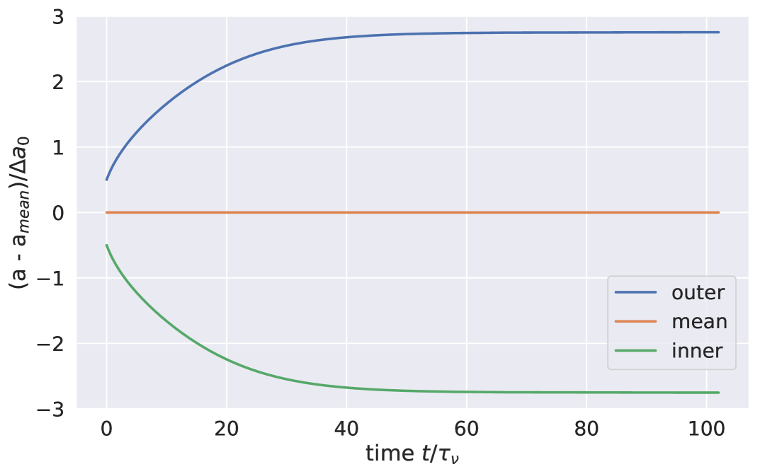
Figure 1: Evolution of the nominal ringlet’s semimajor axes $a$ versus time $t$ in units of the ringlet’s viscous timescale $\tau_{\nu}=1.3\times 10^{3}$ orbital periods. This ringlet is composed of $N_{s}=2$ streamlines, and the outer (blue) and inner (green) streamlines’ semimajor axes are plotted relative to their mean $a_{\text{mean}}$, and displayed in units of the ringlet’s initial width $\Delta a_{0}=10^{-4}$ in natural units (i.e. $G=M=r_{0}=1$). The simulated ringlet has total mass $m_{r}=10^{-10}$, shear viscosity $\nu_{s}=10^{-13}$, and initial eccentricity $e=0.01$. See Section 3.1 to convert $m_{r}$, $a$ and $\nu_{s}$ from natural units to physical units.

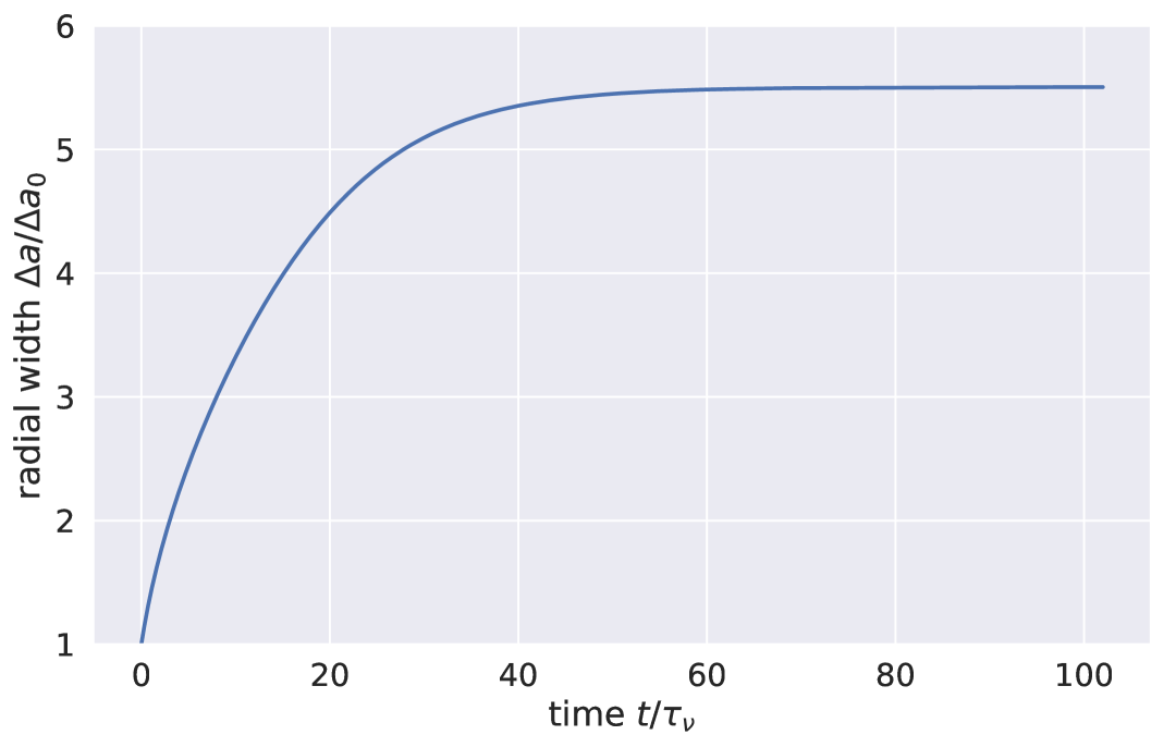
Figure 2: The nominal ringlet’s semimajor axis width $\Delta a=a_{\text{outer}}-a_{\text{inner}}$ over time and in units of its initial radial width $\Delta a_{0}$.

Figure 3 shows that the outer streamline’s eccentricity initially grows at the expense of the inner streamline’s, and that is a consequence the self-gravitating ringlet’s secular perturbations of itself, which is also demonstrated in Appendix C. Figure 4 shows the ringlet’s eccentricity difference $\Delta e=e_{\text{outer}}-e_{\text{inner}}$ and longitude of periapse difference $\Delta\tilde{\omega}=\tilde{\omega}_{\text{outer}}-\tilde{\omega}_{\text{inner}}$, which both settle into equilibrium values after the ringlet arrives at the self-confining state.

In all self-confing ringlet simulations examined here, the ringlet’s periapse twist $\Delta\tilde{\omega}=\tilde{\omega}_{\text{outer}}-\tilde{\omega}_{\text{inner}}$ is negative, so the outer streamline’s longitude of periapse $\tilde{\omega}$ trails the inner streamline’s, which in turn causes the streamlines’ separations along the ringlet’s pre-periapse side (where $\varphi=\theta-\tilde{\omega}<0$) to differ slightly from the post-periapse ($\varphi>0$) side. Which in turn makes the ringlet’s surface density asymmetric i.e. is maximal just prior to periapse, see Figs. 5–6.

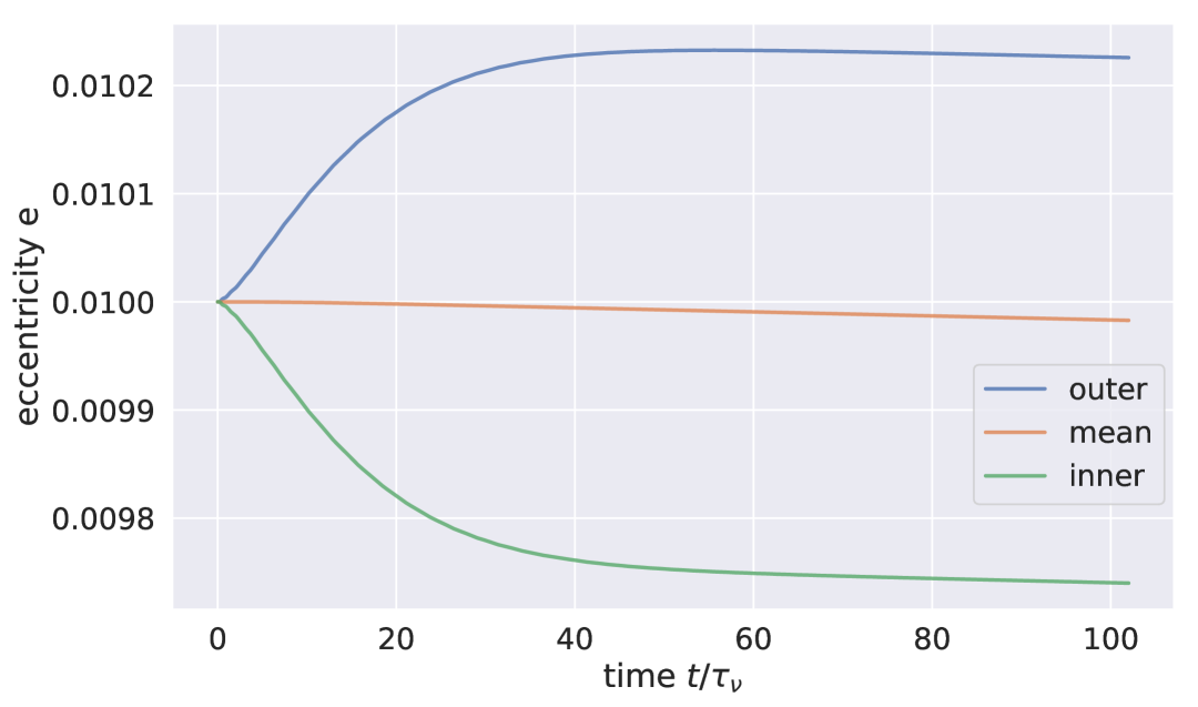
Figure 3: The nominal ringlet’s eccentricity evolution.

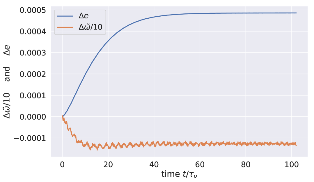
Figure 4: The nominal ringlet’s eccentricity difference $\Delta e=e_{\text{outer}}-e_{\text{inner}}$ and longitude of periapse difference $\Delta\tilde{\omega}=\tilde{\omega}_{\text{outer}}-\tilde{\omega}_{\text{inner}}$ in radians divided by 10.

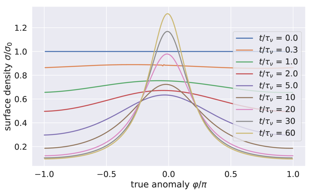
Figure 5: Nominal ringlet’s surface density $\sigma(\varphi)$ versus true anomaly $\varphi$ at selected times $t$ and plotted in units of ringlet’s initial mean surface density $\sigma_{0}$. Note that the ringlet’s surface density maxima occurs just before peripase, and is due to the ringlet’s negative periapse twist $\Delta\tilde{\omega}=\tilde{\omega}_{\text{outer}}-\tilde{\omega}_{\text{inner}}<0$.

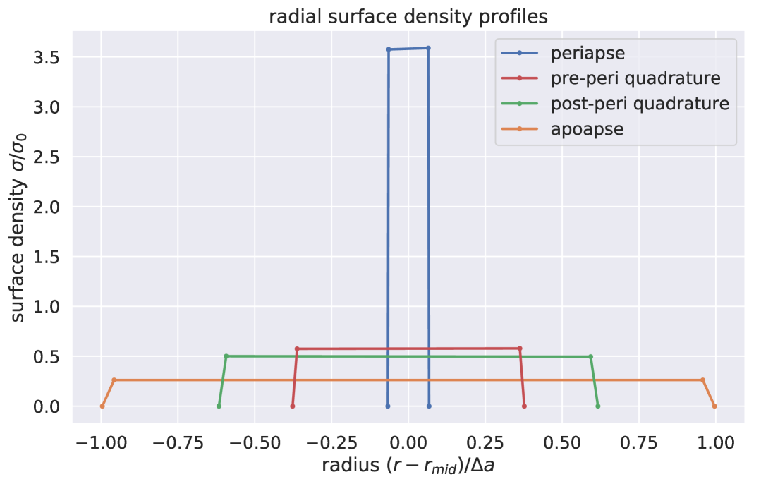
Figure 6: Radial profiles of the nominal ringlet’s surface density $\sigma(\varphi)$ at time $t=100\tau_{\nu}$ when the ringlet is self-confining. Each surface density profile is plotted versus radial distance $r$ relative to $r_{mid}$, which is the ringlet’s midpoint along true anomaly $\varphi=\theta-\tilde{\omega}$, with those radial distances $r-r_{mid}$ measured in units of the ringlet’s final semimajor axis width $\Delta a$, and surface density is shown in units of the ringlet’s longitudinally-averaged surface density $\sigma_{0}$. Radial surface density profiles are plotted along the ringlet’s periapse ($\varphi=0$, blue curve), which is where the ringlet’s streamlines are most concentrated and surface denisity $\sigma$ is greatest due to the ringlet’s eccentricity gradient $e^{\prime}$, at the pre-periapse quadrature ($\varphi=-\pi/2$, red curve), post-periapse quadrature ($\varphi=\pi/2$, green curve) and at apoapse ($|\varphi|=\pi$, orange curve) where streamlines have their greatest separation and ringlet surface density is lowest. This ringlet’s surface density contrast between periapse and apoapse is about 14.

It is convenient to recast these orbit element differences as dimensionless gradients

$$e^{\prime}=a\frac{de}{da}\qquad\mbox{and}\qquad\tilde{\omega}^{\prime}=ea\frac{d\tilde{\omega}}{da}$$ (10)

as these are the terms that contribute to the nonlinearity parameter of Borderies et al. (1983a):

$$q=\sqrt{e^{\prime 2}+\tilde{\omega}^{\prime 2}}.$$ (11)

See also Fig. 7 which plot’s the nominal ringlet’s dimensionless eccentricity gradient $e^{\prime}$, dimensionless periapse twist $\tilde{\omega}^{\prime}$, and nonlinearity parameter $q$ versus time. All simulated self-confining ringlets have a positive eccenticity gradient and a negative periapse twist such that the outer ringlet’s periapse trails the inner ringlet’s, consistent with the findings of Borderies et al. (1983a).

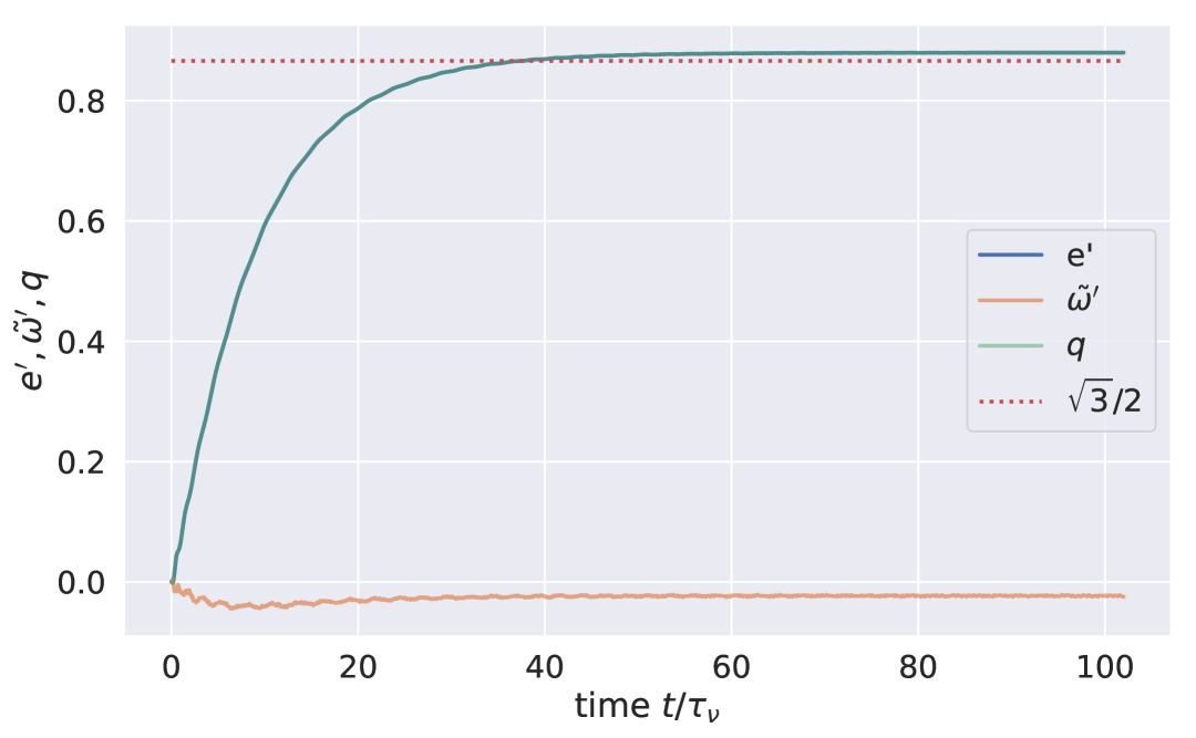
Figure 7: The nominal ringlet’s dimensionless eccentricity gradient $e^{\prime}=a\Delta e/\Delta a$ (blue curve), dimensionless periapse twist $\tilde{\omega}^{\prime}=ea\Delta\tilde{\omega}/\Delta a$ (orange), and nonlinearity parameter $q=\sqrt{e^{\prime 2}+\tilde{\omega}^{\prime 2}}$ (green curve which overlaps blue) versus time $t/\tau_{\nu}$. Dotted red line is the threshold for self-confinement in a non-gravitating ringlet, $e^{\prime}=\sqrt{3}/2\simeq 0.866$

4 angular momentum and energy fluxes & luminosities

The nominal ringlet’s evolution is readily understood when the ringlet’s radial flux of angular momentum and energy are considered.

4.1 angular momentum and energy fluxes

The torque that is exerted on a small streamline segment of mass $\delta m$ at location $\mathbf{r}=r\hat{\mathbf{r}}$ due to the streamlines orbiting interior to it is $\delta T=\delta m\mathbf{r}\times\mathbf{A}^{1}$ where $\mathbf{A}^{1}=A^{1}_{r}\hat{\mathbf{r}}+A^{1}_{\theta}\hat{\boldsymbol{\theta}}$ is the so-called one-sided acceleration that is exerted on $\delta m$ by all other streamlines interior to it. Since $\delta m=\lambda\delta\ell$ where $\lambda$ is the streamline’s linear mass density, and $\delta\ell$ is the segment’s length, then the radial flux of angular momentum flowing into that segment due to the accelerations that are exerted by streamlines interior to that segment is

$${\cal F}_{L}(r,\theta)=\frac{\delta T}{\delta\ell}=\lambda rA^{1}_{\theta},$$ (12)

where $A^{1}_{\theta}$ is the tangential component of the one-sided acceleration, and the streamline’s linear mass density $\lambda$ is computed using Eqn. (2). The radial angular momentum flux, Eqn. (12), is due to the ringlet’s viscosity and self-gravity, so ${\cal F}_{L}={\cal F}_{L,\nu}+{\cal F}_{L,g}$ where

$${\cal F}_{L,\nu}=\lambda rA^{1}_{\nu,\theta}$$ (13)

$$\mbox{and}\quad{\cal F}_{L,g}=\lambda rA^{1}_{g,\theta}$$ (14)

are the viscous and gravitational angular momentum fluxes at a particle. The particle’s one-sided gravitational acceleration $A^{1}_{g,\theta}$ is straightforward to compute, it is merely the tangential component of the gravitational accelerations exerted by all streamlines orbiting interior to the particle, while the viscous angular momentum flux is Eqn. (5) derived in Hahn & Spitale (2013).

The work that the interior streamlines exert on $\delta m$ as that segment travels a small distance $\delta\mathbf{r}=\mathbf{v}\delta t$ in time $\delta t$ is $\delta W=\delta m\mathbf{A}^{1}\cdot\delta\mathbf{r}$ where $\mathbf{v}=v_{r}\hat{\mathbf{r}}+v_{\theta}\hat{\boldsymbol{\theta}}$ is the segment’s velocity, and that work accrues at $\delta m$ at the rate $\delta W/\delta t=\lambda\mathbf{A}^{1}\cdot\mathbf{v}\delta\ell$, so the radial flux of energy entering that ringlet segment due to accelerations exerted by the interior streamlines is

$${\cal F}_{E}(r,\theta)=\frac{\delta W}{\delta\ell\delta t}=\lambda\mathbf{A}^{1}\cdot\mathbf{v}.$$ (15)

The radial energy flux is due to the ringlet’s viscosity and self-gravity, so ${\cal F}_{E}={\cal F}_{E,\nu}+{\cal F}_{E,g}$.

4.2 luminosities

The streamline containing segment $\delta m$ has semimajor axis $a$, and integrating the radial angular momentum flux ${\cal F}_{L}$ about the entire streamline then yields the radial luminosity of angular momentum entering streamline $a$,

$${\cal L}_{L}(a)=\oint{\cal F}_{L}d\ell,$$ (16)

which is the torque that is exerted on streamline $a$ by those orbiting interior to it. Similarly, integrating the radial energy flux ${\cal F}_{E}$ about streamline $a$ also yields the ringlet’s radial energy luminosity

$${\cal L}_{E}(a)=\oint{\cal F}_{E}d\ell,$$ (17)

which is the rate that the interior streamlines communicate energy to streamline $a$.

4.3 viscous transport of angular momentum

Angular momentum is transported radially through the ring via viscosity and self-gravity, so ${\cal F}_{L}={\cal F}_{L,\nu}+{\cal F}_{L,g}$, where the ringlet’s viscous flux of angular momentum is

$${\cal F}_{L,\nu}(r,\theta)=-\nu_{s}\sigma r^{2}\frac{\partial\omega}{\partial r}$$ (18)

when Eqn. (5) is written as a function of spatial coordinates and angular velocity $\omega=\dot{\theta}$. The ring’s surface density $\sigma$ is Eqn. (4) where $\Delta r\simeq\Delta a(1-e^{\prime}\cos\varphi)$ when it is assumed that the ringlet’s eccentricity $e$ is small but its eccentricity gradient $e^{\prime}=a\partial e/\partial a$ might not be, so

$$\sigma\simeq\frac{\sigma_{0}}{1-e^{\prime}\cos\varphi}$$ (19)

where $\sigma_{0}=\lambda/\Delta a$ would be the ringlet’s initial surface density assuming its initial $e^{\prime}$ was zero and $\varphi=\theta-\tilde{\omega}$ is the true anomaly i.e. the longitude relative to periapse. Now consider a small arc of ring material of length $d\ell$, so ${\cal F}_{L,\nu}d\ell$ is the torque that arc exert exerts on ring matter just exterior due to viscous friction, and is the rate that friction transmits angular momentum radially across that arc. And when ${\cal F}_{L,\nu}$ is evaluated along a single eccentric streamline of semimajor axis $a$, the above simplifies to

$${\cal F}_{L,\nu}(a,\varphi)={\cal F}_{L,\nu,c}\frac{1-\frac{4}{3}e^{\prime}\cos\varphi}{(1-e^{\prime}\cos\varphi)^{2}}$$ (20)

where the angular shear $\omega^{\prime}=\partial\omega/\partial r$ in Eqn. (18) is derived in Appendix A, Eqn. (A11), and ${\cal F}_{L,\nu,c}=\frac{3}{2}\nu_{s}\sigma_{0}a\Omega$ is the viscous angular momentum flux through a circular streamline of semimajor axis $a$ that has angular speed $\Omega(a)$. Note that Eqn. (20) is equivalent to Eqn. (18) of Borderies et al. (1982) provided $|\tilde{\omega}^{\prime}|\ll e^{\prime}$ such that $q\simeq e^{\prime}$.

Integrating the above around the streamline’s circumference then yields its angular momentumum luminosity,

$${\cal L}_{L,\nu}(a)=\oint{\cal F}_{L,\nu}(a,\varphi)rd\varphi={\cal L}_{L,\nu,c}\frac{1-\frac{4}{3}e^{\prime 2}}{(1-e^{\prime 2})^{3/2}},$$ (21)

which is the torque that one streamline exerts on its exterior neighbor due to viscous friction (Borderies et al. 1982) with ${\cal L}_{L,\nu,c}=3\pi\nu_{s}\sigma_{0}a^{2}\Omega$ being the viscous angular momentum luminosity of a circular streamline.

Borderies et al. (1982) examine angular momentum transport through a viscous eccentric but non-gravitating ringlet, and use Eqns. (20–21) to show that this transport has three regimes distinguished by the ringlet’s $e^{\prime}$:

1. $e^{\prime}<3/4$. The ringlet’s viscous angular momentum flux ${\cal F}_{L,\nu}(\varphi)>0$ at all longitudes $\varphi$. The ringlet’s viscous angular momentum luminosity ${\cal L}_{L,\nu}>0$, so viscous friction transports angular momentum radially outwards, and the inner ring matter evolves to smaller orbits while exterior ring matter evolves outwards, and the ringlet spreads radially.

2. $3/4\leq e^{\prime}<\sqrt{3}/2$. In this regime there is a range of longitudes $\varphi$ where the viscous angular momentum flux is reversed such that ${\cal F}_{L,\nu}(\varphi)<0$. That angular momentum flux reversal is due to the $\partial\omega/\partial r$ term in Eqn. (5) changing sign near periapse when $e^{\prime}>0.75$, see Fig. 8. Nonetheless ${\cal L}_{L,\nu}$, which is proportional to the orbit-average of ${\cal F}_{L,\nu}(\varphi)$, is positive and the ringlet still spreads radially, albeit slower than when $e^{\prime}<0.75$.

3. $e^{\prime}\geq\sqrt{3}/2$. Viscous angular momentum flux reversal is complete such that ${\cal L}_{L,\nu}\leq 0$, viscous friction transports angular momentum radially inwards, and the ringlet shrinks radially. But if $e^{\prime}=\sqrt{3}/2\simeq 0.866$ then ${\cal L}_{L,\nu}=0$ and the ringlet’s radial evolution ceases, and the viscous but non-gravitating ringlet is self–confining.

Note though that the nominal ringlet’s eccentricity gradient exceeds the $e^{\prime}=\sqrt{3}/2\simeq 0.866$ threshold (dotted red line in Fig. 7) when it settles into self-confinement. This is due to the ringlet’s self-gravity, which also transports a flux of angular momentum ${\cal F}_{L,g}$ radially through the ringlet.

Figure 9 shows the nominal ringlet’s viscous angular momentum flux ${\cal F}_{L,\nu}$ versus true anomaly $\varphi=\theta-\tilde{\omega}$ at selected times $t$. Early in the ringlet’s evolution when time $t\leq 10\tau_{\nu}$ (blue, orange, green, red, purple and brown curves), the ringlet is in regime 1 since $e^{\prime}<0.75$ and ${\cal F}_{L,\nu}(\varphi)>0$ at all longitudes. But by time $t\geq 20\tau_{\nu}$ (pink curve), this ringlet’s eccentricity gradient exceeds $0.75$, and angular momentum flux reversal ${\cal F}_{L,\nu}(\varphi)<0$ occurs near periapse where $|\varphi|\simeq 0$ where the ringlet is most overdense due to its eccentricity gradient, see also Fig. 6. This ringlet is now in regime 2 and its radial spreading is reduced by angular momentum flux reversal. And by time $t=60\tau_{\nu}$ (yellow curve), this ringlet is seemingly in regime 3 since $e^{\prime}>0.866$, so one might expect the ringlet to start contracting now, but keep in mind that the above analysis ignores any transport of angular momentum via ringlet self–gravity. Figure 2 in fact shows that this gravitating ringlet’s spreading had ceased by time $t\simeq 80\tau_{\nu}$, at which point $e^{\prime}=0.88$ (Fig. 9 yellow curve), angular momentum flux reversal is nearly complete, and the ringlet’s total angular momentum luminosity ${\cal L}_{L}={\cal L}_{L,\nu}+{\cal L}_{L,g}$ is very close to zero. Figures 10 and 11 also show that, when the ringlet is self-confining at times $t\geq 80\tau_{\nu}$, its small but positive viscous angular momentum luminosity ${\cal L}_{L,\nu}\simeq 0.006{\cal L}_{L,\nu,c}$ is counterbalanced by its negative gravitational angular momentum luminosity ${\cal L}_{L,g}\simeq-0.006{\cal L}_{L,\nu,c}$, so radial spreading has ceased and the ringlet is self-confining.

Figure 8: The nominal ringlet’s angular shear $\partial\omega/\partial r$ is plotted versus true anomaly $\varphi$ at selected moments in time; this quantity is negative where the inner streamline has the higher angular speed $\omega=v_{\theta}/r$. When the simulation starts, the ringlet has eccentricity $e=0.01$ and eccentricity gradient $e^{\prime}=0$ so $\partial\omega/\partial r\simeq-3\Omega/2r\simeq-1.5$ when evaluated natural units (blue curve). The ringlet’s $e^{\prime}$ then grows over time (orange, green, red curves), which reverses the sign of $\partial\omega/\partial r$ near periapse when $e^{\prime}>0.75$; here the inner ringlet’s angular speed is slower than the outer ringlet, and viscous friction causes angular momentum to instead flow inwards at these longitudes. Dashed curve is Eqn. (A11) with $e^{\prime}=\sqrt{3}/2$ and assuming $|\tilde{\omega}^{\prime}|\ll 1$.

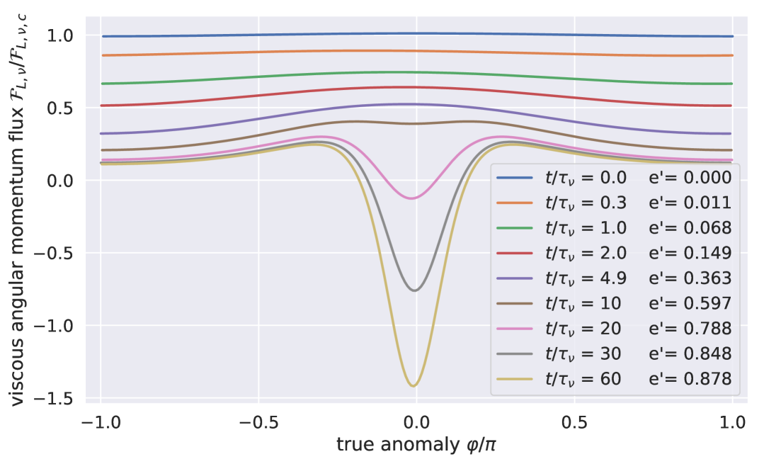
Figure 9: The nominal ringlet’s viscous angular momentum flux ${\cal F}_{L,\nu}(\varphi)$, Eqn. (20), is plotted in units of ${\cal F}_{L,\nu,c}$ (the angular momentum flux in a circular ringlet) and versus the ringlet’s true anomaly $\varphi=\theta-\tilde{\omega}$ at selected times $t/\tau_{\nu}$, with the ringlet’s eccentricy gradient $e^{\prime}$ also indicated.

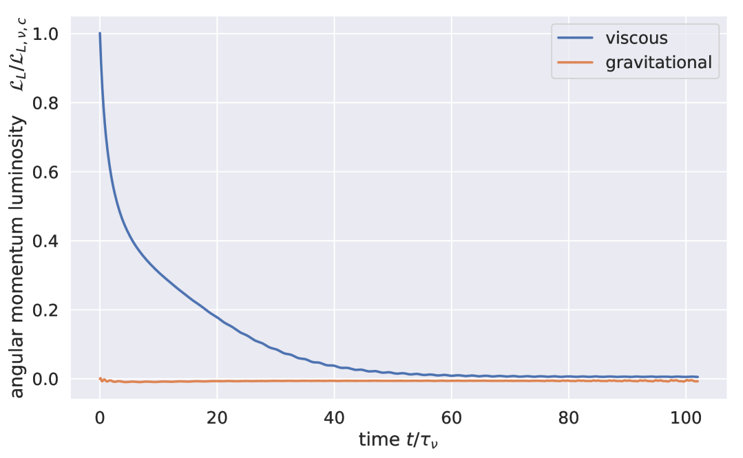
Figure 10: Nominal ringlet’s viscous angular momentum luminosity ${\cal L}_{L,\nu}$ (blue curve) versus time $t/\tau_{\nu}$ and in units of a circular ring’s viscous angular momentum luminosity ${\cal L}_{L,\nu,c}$, as well as the ringlet gravitational angular momentum luminosity ${\cal L}_{L,g}$ (orange curve).

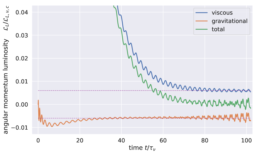
Figure 11: Figure 10 is replotted to show that the ringlet’s viscous angular momentum luminosity ${\cal L}_{L,\nu}$ (blue curve) always stays positive (indicating that the viscous transport of angular momentum is radially outwards) and is eventually balanced by the ringlet’s negative (i.e. inwards) gravitational angular momentum luminosity ${\cal L}_{L,g}$ (orange) after time $t\geq 80\tau_{\nu}$. Green curve is total angular momentum luminosity ${\cal L}_{L,\nu}+{\cal L}_{L,g}$ whose time-average is zero when $t\geq 80\tau_{\nu}$. Dashed lines are $\pm 0.006{\cal L}_{L,\nu,c}$.

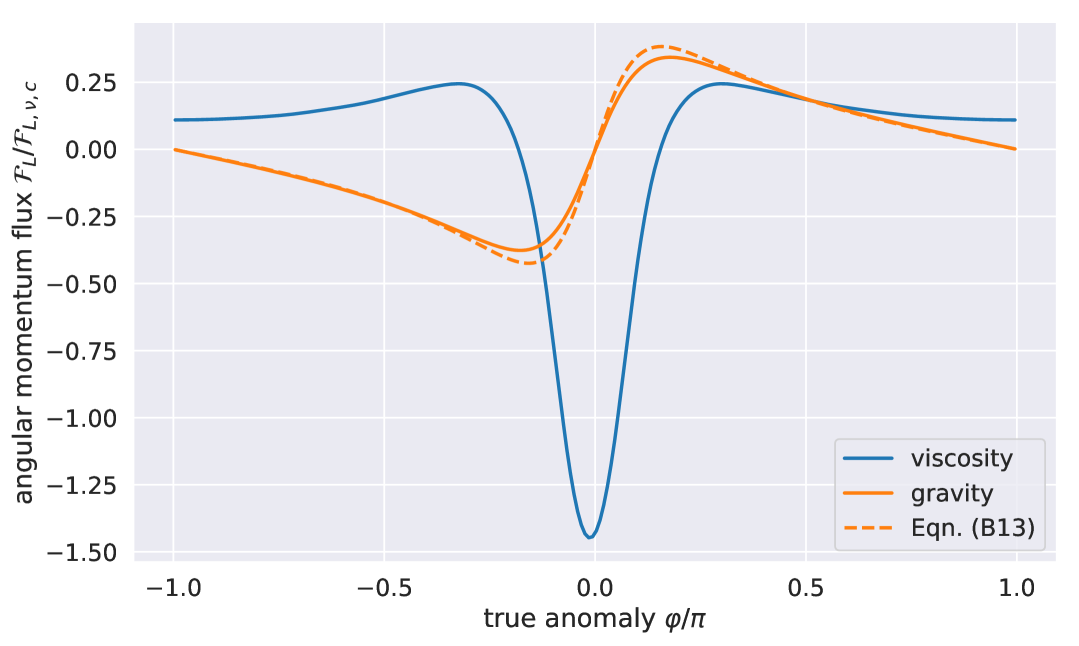
Figure 12: The nominal ringlet’s viscous angular momentum flux ${\cal F}_{L,\nu}(\varphi)$ (blue curve) is computed via Eqn. (5) and plotted in units of a circular ringlet’s flux ${\cal F}_{L,\nu,c}$ versus true anomaly $\varphi$ at the simulation’s end time $t=100\tau_{\nu}$, as well as the ringlet’s gravitational angular momentum flux ${\cal F}_{L,g}(\varphi)$ (orange curve) computed via Eqns. (1) and (14). Dashed curve show the approximate gravitational flux, Eqn. (B2), which is derived in Appendix B agrees very well with the exact flux (solid curve) that is derived from this simulation.

4.4 gravitational transport

The nominal ringlet’s viscous ${\cal F}_{L,\nu}$ and gravitational ${\cal F}_{L,g}$ angular momentum fluxes are shown Fig. 12 after it has settled into the self-confining state. That figure shows how viscous friction tends to transport angular momentum radially inwards, ${\cal F}_{L,\nu}(\varphi)<0$, at longitudes nearer periapse where $|\varphi|\sim 0$, and outwards at all other longitudes, with that flux reversal being due to the reversal of the ringlet’s angular velocity gradient, Fig. 8. Figure 12 also shows that the ringlet’s gravitational transport of angular momentum is inwards as ring-matter approaches periapse where $\varphi<0$, and is outwards ${\cal F}_{L,g}(\varphi)>0$ post-periapse, with that asymmetry being due to the ringlet’s negative periapse twist, $\tilde{\omega}^{\prime}<0$ (Fig. 7). See also Appendix B, which derives the ringlet’s gravitational angular momentum flux ${\cal F}_{L,g}(\varphi)$ as a function of its eccentricity gradient $e^{\prime}$.

Figure 13 shows the ringlet’s energy fluxes due to viscosity (blue curve) and gravity (orange) at simulation end. Integrating these fluxes about a streamline’s circumference at various times $t$ then yields the the ringlet’s viscous ${\cal L}_{E,\nu}$ and gravitational energy luminosity ${\cal L}_{E,g}$ over time, Fig. 14, where the gravitational energy luminosity is computed via

$${\cal L}_{E,g}(a)=\oint{\cal F}_{E,g}(\varphi)rd\varphi=\oint\lambda r\mathbf{A}^{1}_{g}\cdot\mathbf{v}d\varphi$$ (22)

where $\mathbf{A}^{1}_{g}$ is the one-sided gravitational acceleration experienced by a particle in streamline $a$. Note that even though ${\cal F}_{E,\nu}$ and ${\cal F}_{E,g}$ have very different spatial dependances (see Fig. 13), the influence of the ringlet’s viscosity and gravity still conspire such that their orbit-integrated luminosities ${\cal L}_{E}=\oint({\cal F}_{E,\nu}+{\cal F}_{E,g})rd\varphi$ are zero once the ringlet has settled into the self-confining state.

Figure 14 also shows that the ringlet’s gravitational energy luminosity is zero at all times. Which is to be expected since the streamlines’ gravitating ellipses only interact via their secular perturbations, and secular perturbations do no work (Brouwer & Clemence, 1961), hence ${\cal L}_{E,g}=0$. That this quantity evaluates to zero within $\pm 5\times 10^{-24}$ (in nautural units) can also be regarded as another test of the epi_int_lite integrator’s numerical quality.

Figure 13: Blue curve is the nominal ringlet’s viscous energy flux ${\cal F}_{E,\nu}(\varphi)$, plotted in units of a circular ringlet’s viscous energy flux ${\cal F}_{E,\nu,c}$ and versus the ringlet’s true anomaly $\varphi$ at the simulation’s end time $t=100\tau_{\nu}$, as well as the ringlet’s gravitational energy flux ${\cal F}_{E,g}(\varphi)$.

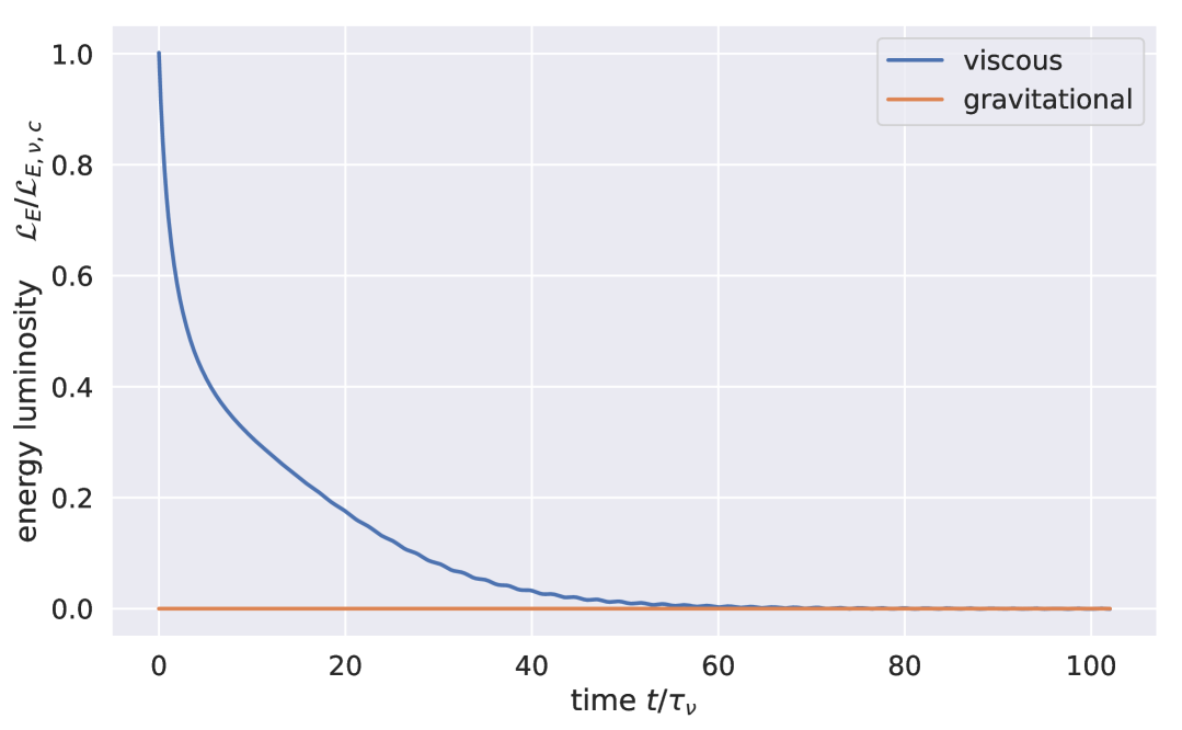
Figure 14: Nominal ringlet’s viscous energy luminosity ${\cal L}_{E,\nu}$ (blue curve) versus time $t/\tau_{\nu}$ and in units of a circular ring’s viscous energy luminosity ${\cal L}_{E,\nu,c}$, as well as the ringlet gravitational energy luminosity ${\cal L}_{E,g}$ (orange curve).

4.5 variations with ringlet width, mass, and viscosity

To assess whether the nominal ringlet’s evolution is typical of other ringlets having alternate values of initial width $\Delta a$, total mass $m_{r}$, and shear viscosity $\nu_{s}$, a survey of 571 additional ringlet simulations are executed. These survey ringlets are similar to the nominal ringlet with $N_{s}=2$ streamlines having $N_{p}=241$ particles per streamline, initial eccentricity $e=0.01$, initial eccentricity gradient $e^{\prime}=0$, and viscosities $\nu_{b}=\nu_{s}$. But the survey ringlets instead have total masses that are geometrically distributed between $10^{-14}\leq m_{r}\leq 10^{-9}$, shear viscosities distributed between $10^{-15}\leq\nu_{s}\leq 10^{-11}$, and initial radial widths distributed between $2.5\times 10^{-5}\leq\Delta a\leq 2.0\times 10^{-4}$. Survey results are summarized in Fig. 15 where circles indicate those ringlets that do evolve into a self-confining state. All simulations of self-confining ringlets are evolved in time until $10\tau_{dyn}$ where the so-called dynamical time $\tau_{dyn}$ is the moment when the ringlet’s nonlinearity parameter $q$ first exceeds $0.6$, since Fig. 7 suggests that $10\tau_{dyn}$ is sufficient time to assess whether the ringlet has truly arrived at the self-confining state.

Figure 15: Outcomes for 572 ringlet simulations having a variety of ringlet masses $m_{r}$ and shear viscosities $\nu_{s}$, with each panel showing results for those ringlets having the same initial radial width $\Delta a=2.5\times 10^{-5}$, $5\times 10^{-5}$, $1\times 10^{-4}$, or $2\times 10^{-4}$. Circles indicate those ringlets that evolve into the self-confining state, while an $\times$ is for those simulations that terminate early when an epi_int_lite particle crossed an adjacent streamline, and N indicates the nominal ringlet simulation. The color of each self-confining ringlet shows whether the ringlet settled into a high–eccentricity gradient state with $e^{\prime}>0.8$ (blue), or smaller eccentricity gradients $0.13>e^{\prime}>0.8$ (cyan), $0.037>e^{\prime}>0.13$ (green), or $e<0.037$ (yellow). All simulations are evolved for the greater of ten dynamical timescales $\tau_{dyn}$ or ten viscous timescales $10\tau_{\nu}$. The middle-right plot is redundant and is here to trick latex into rendering all plots on same page, please ignore.

The $\times$ simulations in Fig. 15 terminated early when an epi_int_lite particle crossed a neighboring streamline. In reality, strong pressure forces would have developed as adjacent streamlines converged and enhanced particle densities and particle collisions, with ring particles possibly rebounding off this high-density region and/or splashing vertically, none of which is accounted for with this version of epi_int_lite. So this survey simply terminates all such simulations and flags that occurrence with an $\times$ in Fig. 15. Keep in mind though that this does not mean that those particular ringlets would not have evolved into a self-confining state. Instead, the streamlines in these ringlets have evolved so close to each other that a more sophisticated and possibly nonlinear treatment of pressure effects would have been needed in order to accurately assess their fates.

Each circle in Fig. 15 represents a self-confining ringlet whose nonlinearity parameter settles into a value that is close to the anticipated value, $q\simeq 0.9$. But these self-confining ringlets’ final eccentricity gradients $e^{\prime}$ also settle into a spectrum of values, $0\leq e^{\prime}\leq 0.9$, with outcomes indicated by circle color in Fig. 15: blue for a high–eccentricity gradient ringlets having $e^{\prime}>0.8$, cyan for smaller eccentricity gradients $0.13>e^{\prime}>0.8$, green for $0.037>e^{\prime}>0.13$, and yellow for very low eccentricity gradients $e<0.037$, with these intervals chosen so that there are approximately 60 simulations in each color-bin. Inspection of Fig. 15 also shows that ringlets having lower $e^{\prime}$ have lower masses and higher viscosities than the higher $e^{\prime}$ ringlets.

Figure 16 shows how eccentricity gradient varies over time $t/\tau_{dyn}$ for a sample of self-confining ringlet simulations. That Figure also shows that the range of simulated $e^{\prime}$ outcomes also agrees with the range of eccentricity gradients observed among several of Saturn’s more well-studied narrow eccentric ringlets, namely the Maxwell, Titan, and Laplace ringlets, whose $e^{\prime}$ are indicated by the black horizontal lines. Figure 16 also shows there is a pileup of simulated outcomes near Laplace’s eccentricity gradient $e^{\prime}\simeq 0.04$, as well as a dearth of simulations at significantly lower values of $e^{\prime}$. Which indicates that the Huygens ringlet, whose $e^{\prime}\lesssim 0.01$, can not be accounted for by the self-confining mechanism considered here.

Also keep in mind that Fig. 16 is not an apples-to-apples comparison of simulated ringlets to observed ringlets, since no attempt is made here to match the observed ringlet’s semimajor-axis width $\Delta a$ to the simulated ringlet’s final $\Delta a$. Rather, Fig. 16’s main point is that many of the observed narrow eccentric ringlets that have $e^{\prime}\gtrsim 0.04$ are consistent with this model of a viscous self-gravitating ringlet that is also self-confining. And lastly, recall that $q=\sqrt{e^{\prime 2}+\tilde{\omega}^{\prime 2}}$ which tells us that lower eccentricity gradient ringlets have a larger periapse twist $|\tilde{\omega}^{\prime}|$.

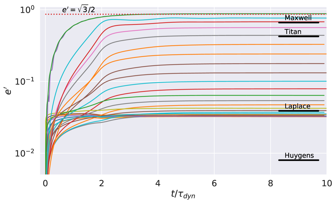
Figure 16: Eccentricity gradient $e^{\prime}$ versus time $t/\tau_{dyn}$ for a sample of 28 self-confining ringlets such that their eccentricity gradients $e^{\prime}$ span the range of values exhibited by the simulations reported in Fig. 15. The ringlet’s dynamical timescale $\tau_{dyn}$ is time the when its nonlinearity parameter $q$ exceeds $0.6$. Sample ringlets have initial $2.5\times 10^{-5}\leq\Delta a\leq 2.0\times 10^{-4}$, $10^{-14}\leq m_{r}\leq 10^{-10}$, and $10^{-14}\leq\nu_{s}\leq 10^{-11}$. Horizontal black lines indicated the observed eccentricity gradients exhibited by the Maxwell, Titan, Laplace, and Huygens ringlets at Saturn (Nicholson et al. 2014, French et al. 2016b, Spitale & Hahn 2016). Dotted line is the $e^{\prime}=\sqrt{3}/2$ threshold.

We also note the French et al. (2024) study of the Uranian ringlets (abbreviated here as F24) which reports observed values for $e^{\prime}$ and $\tilde{\omega}^{\prime}$ for nine ringlets; see quantities $q_{em}=e^{\prime}$ and $q_{\tilde{\omega}m}=\tilde{\omega}^{\prime}$ for the $m=1$ rows in Table 14 of F24. Nearly all of the ringlets monitored in F24 have nonlinearity parameters $q=\sqrt{q_{em}^{2}+q_{\tilde{\omega}m}^{2}}<0.66$ that are significantly smaller than the $q\simeq 0.9$ achieved by the self-confining ringlets simulated here. From this we conclude that the Uranian ringlets are unlike those simulated here.

4.5.1 variations with ringlet viscosity

Figure 17 shows the periapse twist $\tilde{\omega}^{\prime}\simeq ea\Delta\tilde{\omega}/\Delta a$ versus time for six ringlets having the same initial $e_{0}$, $\Delta a$, $m_{r}$ and $\nu_{b}$ as the nominal ringlet but with differing shear viscosities $\nu_{s}$, and that plot shows that twist $|\tilde{\omega}^{\prime}|$ varies with $\nu_{s}$. Which indicates that if the twist $|\tilde{\omega}^{\prime}|$ could be observed in a self-confining ringlet, then the ringlet’s viscosity could then be inferred.

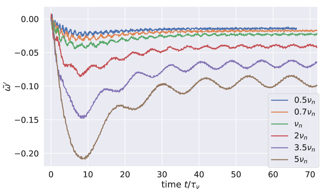
Figure 17: Periapse twist $\tilde{\omega}^{\prime}$ is plotted versus time $t/\tau_{\nu}$ for six ringlets having the same initial $e_{0}$, $\Delta a$, $m_{r}$ as the nominal ringlet but differing shear viscosities $\nu_{s}$ that range over $0.5\nu_{n}\leq\nu_{s}\leq 5\nu_{n}$ where $\nu_{n}=1.0\times 10^{-13}$ is the nominal ringlet’s shear visocity. The time-evolution of these ringlets’ other orbit elements, $\Delta a$, $e$, $e^{\prime}$, and $q$, are very similar to that exhibited by the nominal ringlet, Figs. 2–7.

4.5.2 variations with initial eccentricity

Additional simulations illustrate how outcomes depend upon the ringlet’s initial eccentricity $e_{0}$. Figure 18 shows seven simulations of the nominal ringlet that all have identical physical properties (mass $m_{r}$, viscosity $\nu_{s}$, and initial width $\Delta a$) but differing initial $e_{0}$ ranging over $0\leq e_{0}\leq 0.04$. That plot shows that higher-$e$ ringlets settle into the self-confining state sooner than the lower-$e$ ringlets. This is because the higher-$e$ ringlet’s secular gravitational perturbation of itself drives its eccentricity gradient and hence $q$ towards $q\simeq\sqrt{3}/2$ faster than the lower-$e$ ringlets. Consequently, higher-$e$ ringlets tend to be narrower than lower-$e$ ringlets because they will have had less time to spread before settling into self-confinement. Also note that the $e_{0}=0$ ringlet (blue curve) experiences zero secular gravitational perturbations, so its $q$ is always zero and is destined to spread forever.

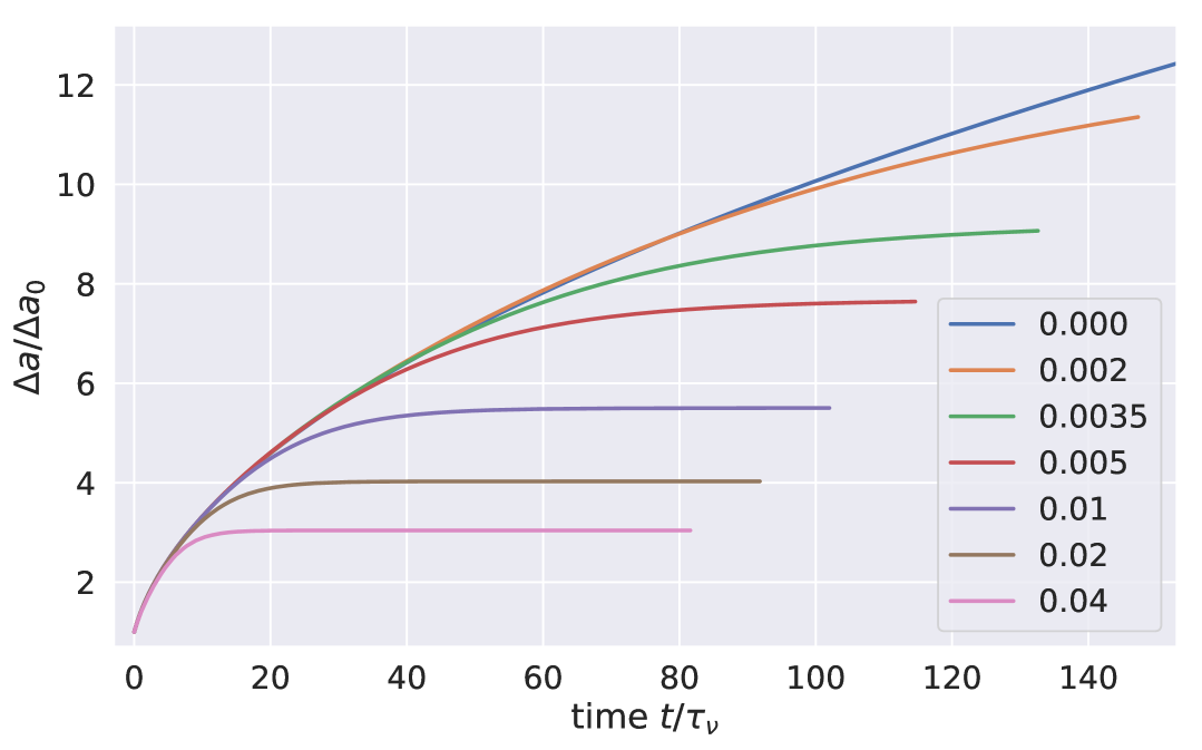
Figure 18: Simulations of seven nominal ringlets having a variety of initial eccentricities $0\leq e_{0}\leq 0.04$. Curves show each ringlet’s semimajor axis width $\Delta a$ in units of its initial $\Delta a_{0}$ versus time $t/\tau_{\nu}$, and show that higher-$e$ ringlets settle into self-confinement sooner than the lower-$e$ ringlets.

The next Subsection will examine the rate at which a self-confining ringlet’s eccentricity $e$ decays over time due to viscosity, and all ringlets shown in Figs. 1–16 have eccentricities $e$ that decay at the expected rates.

4.6 eccentricity damping

Viscous friction within the ringlet is a result of dissipative collisions among ringlet particles. Particle collisions generate heat that is radiated into space, and the source of that radiated energy is the ringlet’s total energy $E_{r}=-m_{r}GM/2a+E_{sg}$ where $m_{r}$ is the ringlet’s total mass, $a$ its semimajor axis, and $E_{sg}$ is the ringlet’s energy due to its self gravity which is contant when the ringlet is self-confining. Collisions conserve angular momentum, so the ringlet’s total angular momentum $L_{r}=m_{r}\sqrt{GMa(1-e^{2})}$ is constant so $dL_{r}/dt=0$ implies that

$$\frac{de^{2}}{dt}\simeq\frac{1}{a}\frac{da}{dt}$$ (23)

to lowest order in the ringlet’s small eccentricity $e$. The ringlet’s energy dissipation rate is $\dot{E}_{r}=dE_{r}/dt=m_{r}GM\dot{a}/2a^{2}$ so $\dot{a}\simeq 2\dot{E_{r}}/m_{r}a\Omega^{2}$ and

$$\frac{de^{2}}{dt}\simeq\frac{2\dot{E_{r}}}{m_{r}a^{2}\Omega^{2}}$$ (24)

where $GM\simeq a^{3}\Omega^{2}$ to lowest order in $J_{2}$. Also note that the surface area of energy dissipation within a viscous disk is

$$\delta=-\nu_{s}\sigma(r\omega^{\prime})^{2}$$ (25)

(Pringle 1981) where $\omega=v_{\theta}/r$ is the angular velocity and $\omega^{\prime}=\partial\omega/\partial r$ its radial gradient.

Now consider a small tangential segment within the ringlet whose length is $d\ell=rd\varphi$ where $\varphi$ is the segment’s longitude measured from the ringlet’s periapse and $d\varphi$ is the small segment’s angular extent. The segment’s area is $dA=\Delta rd\ell=r\Delta rd\varphi$ where $\Delta r$ is the ringlet’s radial width. The rate at which that patch’s viscosity dissipates orbital energy is $d\dot{E_{r}}=\delta dA$, so the ringlet’s total energy dissipation rate is $\dot{E}_{r}=\oint d\dot{E_{r}}$ when integrated about the ringlet’s circumference, and so $\dot{E}_{r}=-2\nu_{s}\lambda\int_{0}^{\pi}r^{3}\omega^{\prime 2}d\varphi$ since the ringlet’s linear density $\lambda=\sigma\Delta r\simeq m_{r}/2\pi a$. So the total energy loss rate due to ringlet viscosity becomes

$$\dot{E}_{r}\simeq-\frac{9}{4}I(e^{\prime})m_{r}\nu_{s}\Omega^{2}$$ (26)

when Eqn. (A11) is used to replace $\omega^{\prime}$, and the integral

$$I(e^{\prime})=\frac{1}{\pi}\int_{0}^{\pi}\left(\frac{1-\frac{4}{3}e^{\prime}\cos\varphi}{1-e^{\prime}\cos\varphi}\right)^{2}d\varphi.$$ (27)

Note that $I(e^{\prime})$ is of order unity except when $e^{\prime}$ is very close to 1, and numerical evaluation shows that $I(e^{\prime})\simeq 0.889$ when $e^{\prime}=\sqrt{3}/2$.

Inserting Eqn. (26) into (24) then yields the rate at which $e^{2}$ is damped,

$$\frac{de^{2}}{dt}=-\frac{9I\nu_{s}}{2a^{2}}$$ (28)

which is easily integrated to obtain

$$e(t)=e_{0}\sqrt{1-\frac{t}{\tau_{e}}}$$ (29)

where $e_{0}$ is the ringlet’s initial eccentricity and

$$\tau_{e}=\frac{2a^{2}e_{0}^{2}}{9I\nu_{s}}$$ (30)

is the ringlet’s eccentricity damping timescale. These expectations are also confirmed in Fig. 19, which plots $e(t)/e_{0}$ versus time $t/\tau_{e}$ for the sample of 28 simulations shown in Fig. 16, with the dashed curve indicating the theoretial predictions of Eqns. (29–30). That all simulated curves have slopes similar to the dashed line tells us that Eqns. (29–30) are a good indicator of outcomes across a wide variety of ringlet parameters.

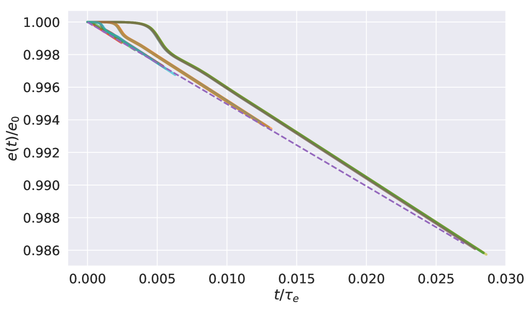
Figure 19: Plot of $e(t)/e_{0}$ versus time $t/\tau_{e}$ for the sample of 28 simulations shown in Fig. 16, while the dashed curve is the expected behavior, Eqn. (29). This sample of simulations have $\tau_{e}$ ranging over $2.5\times 10^{6}\leq\tau_{e}\leq 2.5\times 10^{9}$.

So viscosity circularizes the ringlet in time $\tau_{e}$, during which time the ringlet’s semimajor axis will have shrunk by $\Delta a=\dot{a}\tau_{e}=-e_{0}^{2}a$ by Eqns (23) and (28), so the ringlet’s fractional drift inwards due to viscous damping is

$$\frac{\Delta a}{a}=-e_{0}^{2},$$ (31)

which is small. And after the ringlet’s inner edge damps to zero, its eccentricity gradient $e^{\prime}$ will then shrink over time, angular momentum flux reversal will diminish, and the ringlet’s viscous spreading will resume. So self-confinement of narrow eccentric ringlets is only temporary after all, until time $\tau_{e}$ has elapsed, which is $\tau_{e}/2\pi\sim 1.6\times 10^{6}$ orbits for the nominal model considered here, which is only $\sim 10^{3}$ years for a ringlet orbiting at $a\sim 10^{10}$ cm about Saturn. Recall from Section 3.1 that the viscous lifetime of a non-self-confining nominal ringlet is only $\tau_{\nu}/2\pi\sim 500$ orbits, so self-confinement evidently extends the lifetime of a narrow eccentric ringlet by an additional factor of $\sim 3000$. But self-confinement does not solve the ringlet’s lifetime problem, because self-confinement is ultimately defeated by viscous damping of the ringlet’s eccentricity.

4.7 number of streamlines $N_{s}$

When the simulated ringlet is composed of $N_{s}=2$ streamlines, the ringlet’s evolution is largely analytic (c.f. Borderies et al. 1982, 1983a), and the analytic predictions provide excellent benchmark tests for the epi_int_lite integrator. This subsection assesses whether the results obtained for the simpler $N_{s}=2$ ringlet also apply to more realistic ringlets having $N_{s}>2$.

Figures 20–21 recomputes the nominal ringlet’s evolution for ringlets having a range of streamlines, $2\leq N_{s}\leq 14$, all of which have $q$-evolution very similar to that exhibited by the $N_{s}=2$ simulation seen in Fig. 7. Figure 20 plots each streamline’s eccentricity $e$ versus their relative semimajor axis $\Delta a=a-\bar{a}$, which shows that all simulated ringlet’s have the same eccentricity gradient $e^{\prime}$ regardless of the number of streamlines $N_{s}$. Ditto for the ringlets’ relative longitudes of periapse, $\Delta\tilde{\omega}$ when plotted versus $\Delta a$, Fig. 21, which shows that all simulated ringlets have comparable gradients in $\tilde{\omega}$. The only noteworthy difference seen here is that the smaller $N_{s}\leq 3$ simulations do not resolve the extra peripase twist that is seen at the edges of the higher resolution simulations. Except for this one distinction, the evolution of the $N_{s}>2$ ringlets are very similar to that exhibited by nominal ringlet composed of $N_{s}=2$ streamlines.

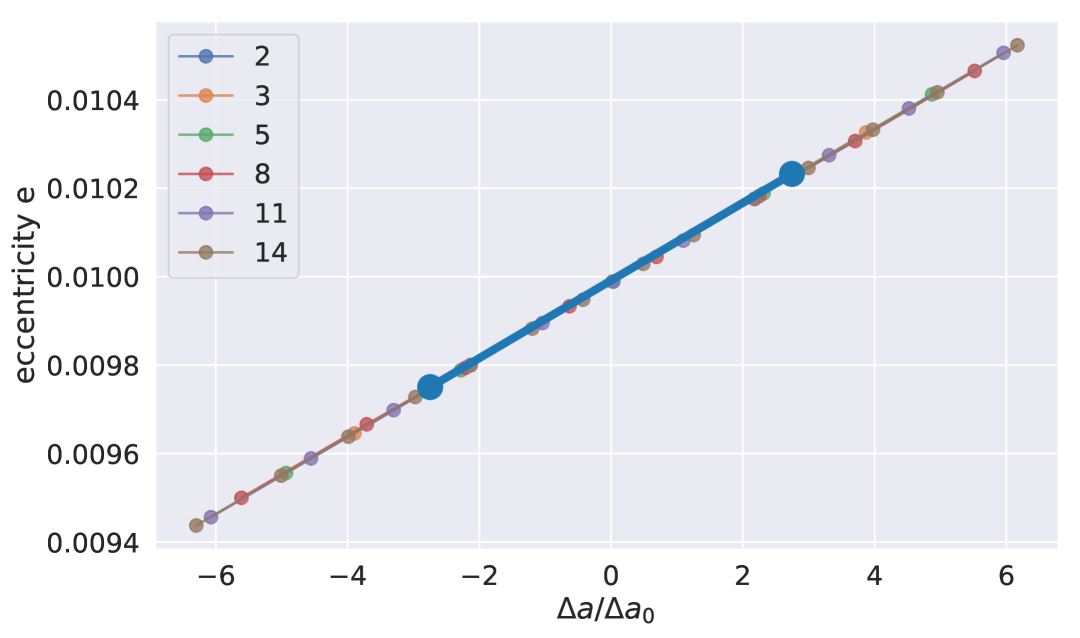
Figure 20: A suite of ringlets are evolved, these ringlets have the same properties as the nominal ringlet except they contain varied numbers of streamlines $2\leq N_{s}\leq 14$, with $N_{s}$ indicated by the plot legend. Simulated ringlets’ final eccentricities $e$ are plotted versus their relative semimajor axis $\Delta a=a-\bar{a}$ where $\bar{a}$ is the ringlet’s mean semimajor axis.

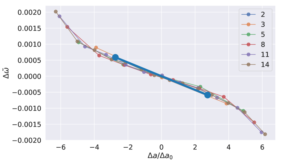
Figure 21: Simulated ringlets’ final relative longitudes of periapse $\Delta\tilde{\omega}=\tilde{\omega}-\bar{\omega}$ are plotted versus their relative semimajor axis $\Delta a=a-\bar{a}$, where $\bar{a}$ is the ringlet’s mean semimajor axes and $\bar{\omega}$ is their mean longitude of periapse, and number of streamlines $N_{s}$ is indicated in the plot legend.

4.7.1 surface densities and sharp edges

The main shortcoming of the $N_{s}=2$ simulation is that it reveals nothing about a ringlet’s possible sharp edges, since a two-streamline ringlet always has artificially sharp edges. To examine this further, Fig. 22 shows the radial surface density profile along the periapse direction for the $2\leq N_{s}\leq 14$ ringlets that were simulated in Section 4.7. That plot shows that all ringlets’ edges are sharp after they arrive in the self-confining state, regardless of $N_{s}$. When self-confining, each streamline is approximately equidistant (within $25\%$) from their neighbors, which causes ringlet surface density $\sigma$ to be remain constant (within $25\%$) in the ringlet interior, which then plummets to zero beyond the ringlet’s boundaries. Ditto for the surface density profiles seen along the ringlets’ apoapse direction, Fig. 23. In summary, the self-confining ringlet examined here has a smooth radial surface density profile that is concave–down, with surface density maxima at the ringlet’ center, and has sharp edges.

Note that if a vicous ringlet were instead unconfined, then its positive angular momentum flux would have repelled the edgemost streamlines away from the interior streamlines, which in turn would have caused the ringlet’s concave–down surface density profile to taper smoothly to zero at its edges, as is seen in Fig. 1 of Pringle (1981). Meanwhile, the other ringlet models, those that rely on unseen shepherd satellites to maintain confinement, all exhibit smooth surface densities having a variety of concavities, yet all have sharp edges (Goldreich & Tremaine 1979a; Chiang & Goldreich 2000; Mosqueira & Estrada 2002).

In comparison, the Maxwell ringlet’s radial optical depth profiles can be approximately described as concave–downish with a spiral density wave riding on top (Nicholson et al. 2014). The Titan ringlet is opaque so its concavity is unknown, but it does have sharp edges (Nicholson et al. 2014). The Huygens ringlet, which has a tiny eccentricity gradient, is concave–up with sharp edges (French et al. 2016b), while the Laplace ringlet is possibly concave–down with sharp edges and lots of internal structure. Main point: all well-observed narrow eccentric planetary ringlets have a radial optical depth structure that is much more complicated than is exhibited by published models to date.

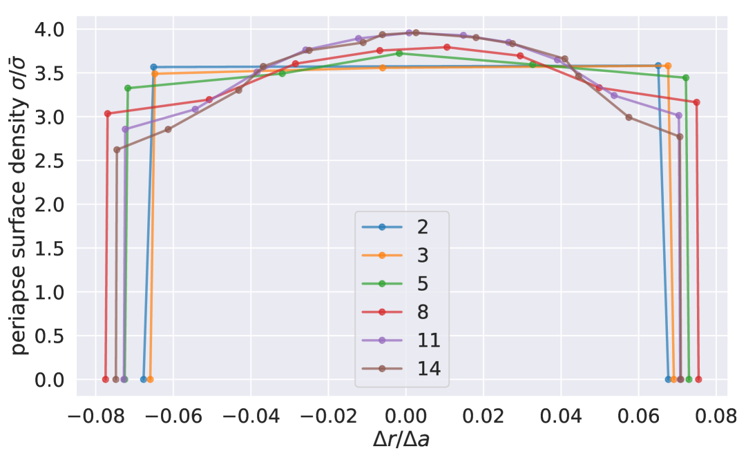
Figure 22: Radial surface density profiles $\sigma(\Delta r)$ of the $2\leq N_{s}\leq 14$ ringlets of Section 4.7 plotted along the ringlets’ direction of periapse. Surface density $\sigma$ is shown in units of the ringlet’s mean surface density $\bar{\sigma}$, and radial distance $\Delta r=r-r_{\text{mid}}$ is measured relative to chord’s midpoint and in unit of the ringlet’s semimajor axis width $\Delta a=a_{\text{outer}}-a_{\text{inner}}$.

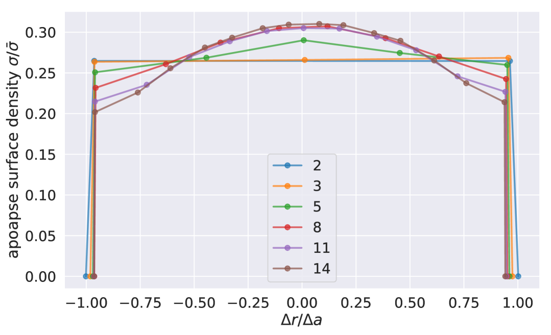
Figure 23: Radial surface density profiles $\sigma(\Delta r)$ of the $2\leq N_{s}\leq 14$ simulations, plotted along the ringlets’ direction of apoapse. Note that the ringlets’ apoapse surface densities are about 13 times smaller than their periapse $\sigma$, Fig. 22, because they are also wider by that amount.

5 self–confining ringlet origin scenario

Here we use the preceding results to speculate about the origin of narrow eccentric planetary ringlets. If such ringlets are truly self-confining, then they are extremely young, only $\sim{\cal O}(1000)$ years old per Eqn. (30) and Section 4.6. Our preferred least-speculative origin scenario (which is still quite speculative) proposes that the ringlet precursor was originally an especially large ring particle that was orbiting elsewhere such as within a nearby dense planetary ring, presumably as an embedded moonlet aka propeller (Tiscareno et al. 2010). If that embedded moonlet happened to form near the edge of the dense planetary ring, then the moonlet’s reaction to the shepherding torque that it exerts across the dense ring [which is $-1\times$ the radial integral of Eqn. (71) of Goldreich & Tremaine (1982)] would cause that moonlet to migrate towards and then beyond the ring’s edge. And if a dense planetary ring can spawn one such moonlet, it can also spawn additional moonlets. Charnoz et al. (2010) also propose such for the origin for all the small satellites orbiting just beyond Saturn’s A ring: Atlas, Prometheus, Pandora, Epimethius, and Janus.

A moonlet’s radial migration rate due to the ring-shepherding torque also varies with moonlet mass, so a larger moonlet will eventually overtake a smaller moonlet that is orbiting beyond it. Indeed, calculations by Poulet & Sicardy (2001) suggest that satellite Prometheus emerged from the outer edge of Saturn’s A ring $\sim 10^{7}$ years ago, and that it will have a close encounter with the smaller satellite Pandora that is currently orbiting just exterior to Prometheus in another $\sim 10^{7}$ years. Multiple close moonlet-moonlet encounters would then pump up moonlet eccentricities until they collide. If that collision is sufficiently vigorous to disrupt one or both moonlets, then a narrow eccentric planetary ringlet composed of collisional debris would result. Viscous particle-particle collisions would then cause that young ringlet to spread radially (Fig. 2) while its self-gravity would pump up its eccentricity gradient (Fig. 7) which, if sufficiently vigorous, would cause it to settle into the self-confining state that is sharp-edged (Fig. 23) like most observed narrow eccentric ringlets. Nonetheless, self-confinement is temporary and lasts only $\sim{\cal O}(1000)$ years due to the ringlet’s viscosity damping its eccentricity until its inner edge gets circularized. Which would would cause the ringlet’s $q$ to drop below the $q\simeq\sqrt{3}/2$ threshold for self-confinement, the ringlet would again spread radially, and its edges would lose their sharpness.

So in summary, this purportedly least-speculative ringlet origin scenario implies that dense planetary rings are frequently forming and emitting small embedded moonlets that then migrate away, due to their gravitational shepherding of that ring, towards and then beyond the nearby ring-edge where they are later disrupted after colliding with other such moonlets. The resulting debris quickly shears out into a low-eccentricity ringlet whose self-gravity excites its eccentricity gradient until it settles temporarily into the self-confining state, which is sharp-edged. The next step in any assessment of the viability of this least-speculative ringlet origin scenario would require estimating the various timescales that are relevant here, namely, the moonlet’s formation timescale, the moonlet’s migration timescale, its lifetime versus collisional disruption, and the ringlet’s self-confinement lifetime, to confirm that none of these lifetimes are so long as to cast doubt on this ringlet origin scenario. That more detailed analysis is deferred to a followup study.

6 summary of findings

Main findings:

1. Simulations show that viscous self-gravitating narrow eccentric ringlets having a wide variety of initial physical properties (mass, width, and viscosity) do evolve into the self-confining state (Fig. 15).

2. Self-gravity causes a self-confining ringlet’s nonlinearity parameter $q$, which is the RMS sum of the ringlet’s dimensionless eccentricity gradient $e^{\prime}=ade/da$ and its dimensionless periapse twist $\tilde{\omega}^{\prime}=ead\tilde{\omega}/da$, to grow over time until it exceeds the $q\simeq\sqrt{3}/2\simeq 0.866$ threshold where the ringlet’s orbit-averaged angular momentum flux due to ringlet viscosity + self-gravity reversal is zero.

3. Gravitating ringlets that are self-confining have small but positive (i.e. radially outwards) viscous angular momentum luminosity that is counterbalanced by its negative gravitational angular momentum luminosity (Section 4.3). Ringlet self-gravity is also the reason for a self-confining ringlet having nonlinearity parameter $q\simeq 0.9$ that is slightly larger than the $q=\sqrt{3}/2\simeq 0.866$ threshold that is expected of a viscous non-gravitating ringlet (Borderies et al., 1982).

4. Simulated ringlets that do settle into self-confinement have final eccentricity gradients $0.04\lesssim e^{\prime}\lesssim 0.9$, Fig. 16. Since all such ringlets have $q\simeq 0.9$, this means that ringlets having smaller eccentricity gradients $e^{\prime}$ also have larger periapse twist $|\tilde{\omega}^{\prime}|$ that is likely due to a higher ringlet viscosity (Section 4.5.1).

5. The ringlet’s total energy luminosity ${\cal L}_{E}$ is zero after the ringlet has settled into the self-confining state (Section 4.4). The ringlet’s gravitational energy luminosity ${\cal L}_{E,g}$ is also zero at all times, consistent with secular theory.

6. Self-confining ringlets have sharp edges (Section 4.7.1).

7. Ringlet viscosity also circularizes the ringlet in time $\tau_{e}\sim 10^{6}$ orbits $\sim 1000$ years (Section 4.6). After viscosity has reduced the eccentricity of the ringlet’s inner edge to zero, the ringlet’s eccentricity gradient $e^{\prime}$ will then shrink over time, its angular momentum flux reversal will cease, and viscous spreading will resume as ringlet viscosity again transmits an outwards flux of angular momentum. Ringlet circularization thus causes it to again resume spreading radially, and the ringlet would lose its sharp edges.

8. Self-confining narrow eccentric planetary ringlets are short lived unless there is a mechanism that can pump up the ringlet’s eccentricity.

9. We speculate that a sharp-edged self-confining narrow eccentric planetary ringlet first originated as an exceptionally large ring particle orbiting within a nearby dense planetary ring. Possibly as a small embedded moonlet such as the presumed cause of the propeller structures seen in Saturn’s main A ring. If that embedded moonlet is orbiting near the dense ring’s edge, then its reaction to the gravitational shepherding torque that it exerts across the dense ring would cause that moonlet to migrate towards and then beyond the dense ring’s edge. If so, then a dense planetary ring can also birth multiple such moonlets. The ring-torque would also cause the largest moonlet to overtake any smaller migrating moonlets, which will encourage moonlet-moonlet scattering and eventual collision. A disruptive moonlet collision would generate debris that would quickly shear out into a low-eccentricity ringlet whose self-gravity could excite its eccentricity gradient until it settles into the self-confining state that is sharp-edged, albeit temporarily.

7 additional followup studies

Here we list possible followup studies that could also be pursued using the epi_int_lite streamline integrator:

1. Nonlinear spiral density waves: analytics theories exist, but they are complex and challenging to employ (Shu et al., 1985; Borderies et al., 1986), whereas some might regard the execution of an epi_int_lite simulation as the simpler/faster way forward. Spiral density waves are nonlinear when the surface density variation due to the wave is comparable to the ring’s undisturbed surface density i.e. $|\Delta\sigma|\sim\sigma_{0}$. Since $\sigma=\lambda/\Delta r$, this means that streamline separation $\Delta r$ need only shrink by a factor of two to make a density wave nonlinear. Note that eccentricities associated with the wave are still small, which means that the streamline-integrator approach is well suited for simulating nonlinear density waves. See for example the French et al. (2016a) simulation of a marginally nonlinear spiral density wave using the epi_int code, which is the predecessor of epi_int_lite.

2. Partly incompressible nonlinear spiral density waves: one can imagine that a sufficiently vigorous nonlinear density wave could drive particle densities high enough such that ring particles in the affected region are packed shoulder-to-shoulder so that further compaction is impossible because that region has becomes incompressible. We suspect that these incompressible patches could also result in shocks and/or vertical splashing as the wave drives additional ring particles into the affected regions. Which surely would alter the wave’s dynamics and may lead to new and possibly observable phenomena (e.g. Borderies et al. 1985). Note that the equation of state (EOS) employed by epi_int_lite assumes that the ring is a compressible particle gas, but that EOS could easily be adapted to account for the additional forces that would result as particles enter into or recoil from the incompressible patches generated by the wave.

3. Nonlinear spiral bending waves: although theories for nonlinear spiral density waves do exist, an analytic theory for a nonlinear spiral bending wave does not. The fundamental assumption of linearized bending wave theory is that the radial forces associated with the wave are negligible compared to the wave’s vertical forcing of the ring (Shu, 1984). Which is true provided the bending wavelength $\lambda_{b}$ is large compared to the bending wave amplitude $A$, which is the ring plane’s maximal vertical displacement due to the bending wave, i.e. $\lambda_{b}\gg A$. Although the epi_int_lite streamline integrator is currently a two dimensional code, adapting it to the 3^rd dimension should be straightforward, which means that the revised code would then be well positioned to simulate a nonlinear spiral bending wave having $\lambda_{b}\lesssim A$. Also note that, when in this regime, the gravitational forces exerted by the warped ring plane are no longer purely vertical i.e. the wave’s forcing of the warped ring-plane within distances $\sim\lambda_{b}$ will also have an in-plane component. And that radial forcing of a self-gravitating ring tends to beget spiral density waves. Which suggests that a spiral bending wave, whose wavelength $\lambda_{b}$ shrinks as it propagates, will eventually go nonlinear in a way that might spawn a spiral density wave that could be observable in Cassini observations of Saturn’s rings.

4. Galactic spiral structure: the main difference between planetary and galactic trajectories is in their precession rates. Planetary orbits precess slowly, $|\dot{\tilde{\omega}}|=|\Omega-\kappa|\ll\Omega$, whereas galactic trajectories, which can also be described by equations like Eqn. (A), precess rapidly, $|\dot{\tilde{\omega}}|\sim\cal{O}($$\Omega)$. Which suggests that epi_int_lite could also be used to simulate galactic spiral stucture when the code is provided with appropriate functions for $\Omega(r)$ and $\kappa(r)$. Epi_int_lite is also quite general in that it can simulate waves in both gravity and pressure dominated disks, and additional perturbations from a central bar would be straightforward to include.

5. Asymmetric circumstellar debris disk: a debris disk is a dusty circumstellar disk that is often found in orbit about younger stars, $\sim 10^{7-9}$ years (Matthews et al., 2018), and is a possible signature of ongoing planet formation. Many such star-disk systems are suspected of hosting an unseen planetesimal ‘birth ring’, wherein collisions among those planetesimals generates dust whose smaller grains are launched into very wide eccentric orbits due to stellar radiation pressure (Strubbe & Chiang, 2006). Those eccentric dust grains populate a very broad disk that can be observed out to stellar-centric distances of $r\sim 1000$ AU when imaged via scattered starlight, which also tends to favor the discovery of edge-on debris disks. These edge-on dust disks’ ansae routinely exhibit surface-brightness asymmetries as well other structures that may be due to gravitational forcing by unseen protoplanets and/or giant impacts into those protoplanets (Jones et al. 2023). Surface-brightness asymmetries can also be due to the birth ring having an eccentricity (Hahn, 2009), which again implicates gravitational forcing by unseen planets or protoplanets, but differential precession due to the protoplanets’ gravities will eventually defeat the birth ring’s eccentricity unless that is resisted by the ring’s self-gravity. The longevity of these possibly eccentric birth rings and their debris disks, which is inferred from their host stars’ $10^{7+}$ yr ages, suggests that these possibly eccentric birth rings can also be very long-lived. Which causes us to wonder whether self gravity may play a role in preserving a birth ring’s structure via the self-confinement mechanism considered here, which epi_int_lite would be well-suited to investigate.

The epi_int_lite streamline integrator source code is available at https://github.com/joehahn/epi_int_lite, and readers are encouraged to reach out if they wish to use that code in their research.

8 Acknowledgments

This research was supported by the National Science Foundation via Grant No. AST-1313013. A portion of this paper as well as the epi_int_lite integrator were composed and developed while at the Water Tank karaoke bar in northwest Austin TX, and the authors thank proprietor James Stryker for his hospitality. The authors also thank Joe Spitale and an anonymous review for their comments about this work.

Appendix A Appendix A

The drift step implemented in the original epi_int code utilized the epicyclic equations of Borderies-Rappaport & Longaretti (1994) to advance an unperturbed particle along its trajectory about an oblate planet. Those equations convert a particle’s spatial coordinates $r,\theta,v_{r},v_{\theta}$ into epicyclic orbit elements $a,e,M,\tilde{\omega}$ that are easily advanced by timestep $\Delta t$, after which the epicyclic elements are converted back to spatial coordinates with an accuracy to ${\cal O}(e^{2})$. Note though that those epicyclic equations are not reversible; every conversion from spatial to epicyclic coordinates or vice-versa also introduces an error of order ${\cal O}(e^{3})$, and the accumulation of those errors causes the orbits of the epi_int particles to slowly drift over time. But that slow numerical drift was not problematic for the relatively short epi_int simulations reported in Hahn & Spitale (2013) that evolved Saturn’s B ring for typically $\sim 10^{4}$ orbit periods. However the viscous self-gravitating ringlets considered here must be evolved for $10^{5}$ to $10^{6}$ orbit periods in order for self-confinement to occur, and simulations having those longer execution times were being defeated by this orbital drift. The remedy is to derive an alternate set of epicyclic equations that are reversible such that the epi_int_lite’s drift step will not be a significant source of numerical error.

Begin with the equation of motion for an unperturbed particle in orbit about the central planet,

$$\ddot{\mathbf{r}}=-\nabla\Phi$$ (A1)

where the planet’s gravitational potential is

$$\Phi=-\frac{GM}{r}-\frac{J_{2}GMR^{2}}{2r^{3}}$$ (A2)

where $M$ is the planet’s mass, $R$ its radius, $J_{2}$ its second zonal harmonic due to oblateness, and with higher-order $J_{n>2}$ terms ignored here. The angular part of Eqn. (A1) is

$$\frac{1}{r}\frac{d}{dt}(r^{2}\dot{\theta})=-\frac{\partial\Phi}{\partial\theta}=0$$ (A3)

so the particle’s specific angular momentum $h=r^{2}\dot{\theta}=rv_{\theta}$ is conserved i.e.

$$\dot{\theta}=\frac{h}{r^{2}},$$ (A4)

and inserting that into the radial part of Eqn. (A1) yields

$$\ddot{r}=\frac{h^{2}}{r^{3}}-\frac{GM}{r^{2}}-\frac{3J_{2}GMR^{2}}{2r^{4}}.$$ (A5)

Solving the above to first-order accuracy ${\cal O}(e^{1})$ ordinarily yields

$$r \simeq a(1-e\cos M)$$

$$\theta \simeq \frac{\Omega}{\kappa}(M+2e\sin M)+\tilde{\omega}$$

$$v_{r}=\dot{r} \simeq ea\kappa\sin M$$

$$v_{\theta}=r\dot{\theta} \simeq a\Omega(1+e\cos M)$$ (A6)

where

$$\Omega(a)=\sqrt{\frac{GM}{a^{3}}}\left[1+\frac{3}{2}J_{2}\left(\frac{R}{a}\right)^{2}\right]^{1/2}$$ (A7)

is the particle’s mean orbital frequency and

$$\kappa(a)=\sqrt{\frac{GM}{a^{3}}}\left[1-\frac{3}{2}J_{2}\left(\frac{R}{a}\right)^{2}\right]^{1/2}$$ (A8)

its epicyclic frequency. In the above, $a$, $e$, $\tilde{\omega}$ and $M=\kappa t$ are the epicyclic orbit elements that have errors of order ${\cal O}(e^{2})$. Equations (A) are easily inverted, which would then provide epicyclic orbit elements $a$, $e$, $\tilde{\omega}$, $M$ as functions of the particle’s spatial coordinates $r$, $\theta$, $v_{r}$, $v_{\theta}$, but applying them here would be even more problematic since the conversion from spatial coordinates to orbit elements would accrue ${\cal O}(e^{2})$ errors during every drift step, which is even worse that the rate at which epi_int’s drift step accrues errors.

The remedy is to choose an alternate set of equations (A) that also solve the equation of motion (A1) to the same accuracy while satisfying Eqn. (A4) exactly. Begin with the above expression for the angular coordinate, $\theta=(\Omega/\kappa)(M+2e\sin M)+\tilde{\omega}$, so that $\dot{\theta}=\Omega(1+2e\cos M)$. Then require the constant $h=r^{2}\dot{\theta}=a^{2}\Omega$ be satisfied exactly, which provides the revised expression for $r$ as a function of orbit elements, $r=a/\sqrt{1+2e\cos M}$, noting that this expression differs from that in Eqn. (A) by an amount of order ${\cal O}(e^{2})$ which is this solution’s allowed error. It is then straightforward to complete the revisions to Eqn. (A):

$$r = \frac{a}{\sqrt{1+2e\cos M}}$$

$$\theta = \frac{\Omega}{\kappa}(M+2e\sin M)+\tilde{\omega}$$

$$v_{r}=\dot{r} = \frac{ea\kappa\sin M}{(1+2e\cos M)^{3/2}}=ea\kappa\sin M\left(\frac{r}{a}\right)^{3}$$

$$v_{\theta}=r\dot{\theta} = a\Omega\sqrt{1+2e\cos M}=\frac{a^{2}\Omega}{r}$$ (A9)

where $\Omega$ and $\kappa$ are Eqns. (A7–A8) and $M=\kappa t$.

Eqns. (A) must also be inverted so that the particle’s epicyclic orbit elements $a,e,\tilde{\omega},M$ can be obtained from the particle’s spatial coordinates $r,\theta,v_{r},v_{\theta}$, which is done via the following:

1. Calculate the particle’s specific angular momentum $h=rv_{\theta}$ and then solve $h^{2}=a^{4}\Omega^{2}=GMa[1+(3J_{2}/2)(R/a)^{2}]$ for the particle’s semimajor axis $a$, which is

   $$a=R\left(C+\sqrt{C^{2}-3J_{2}/2}\right)$$ (A10)

   where constant $C=h^{2}/2GMR$.

2. Calculate $\Omega$ and $\kappa$ using Eqns. (A7–A8).

3. Note that $e\sin M=(v_{r}/a\kappa)(a/r)^{3}$ and $e\cos M=\text@frac{1}{2}[(a/r)^{2}-1]$, which provides the particle’s eccentricity via $e=\sqrt{(e\sin M)^{2}+(e\cos M)^{2}}$ and its mean anomaly $M$ inferred from $\tan M=e\sin M/e\cos M$.

4. The particle’s longitude of periapse is $\tilde{\omega}=\theta-(\Omega/\kappa)(M+2e\sin M)$.

These equations satisfy the equation of motion (A1) to accuracy ${\cal O}(e)$ and with errors of order ${\cal O}(e^{2})$. To advance a particle during epi_int_lite’s drift step from time $t$ to time $t+\Delta t$, use the above steps 1-4 to convert the particle’s spatial coordinates $r,\theta,v_{r},v_{\theta}$ to epicyclic orbit elements $a,e,M,\tilde{\omega}$, update the particle’s mean anomaly via $M\rightarrow\kappa(t+\Delta t)$, and then use Eqns. (A) to compute the particle’s revised spatial coordinates. And because steps 1-4 convert coordinates to elements exactly, epi_int_lite’s drift step is not a significant source of numerical error.

Lastly we derive the streamlines’ angular shear $\partial\omega/\partial r$. The angular velocity $\omega=v_{\theta}/r=\Omega(a/r)^{2}$ by Eqn. (A) so $\omega\simeq\Omega(1+2e\cos\varphi)$ to first order in $e$ where true anomaly $\varphi=\theta-\tilde{\omega}\simeq M$. Thus $\partial\omega/\partial a\simeq-(3\Omega/2a)(1-\frac{4}{3}e^{\prime}\cos\varphi)$ since $J_{2}$ and $e$ are small though the eccentricity gradient $e^{\prime}=a(\partial e/\partial a)$ might not be small. Likewise $r\simeq a(1-e\cos\varphi)$ so $\partial r/\partial a\simeq 1-e^{\prime}\cos\varphi$ and so

$$\omega^{\prime}=\frac{\partial\omega}{\partial r}=\frac{\partial\omega}{\partial a}/\frac{\partial r}{\partial a}\simeq-\left(\frac{3\Omega}{2a}\right)\frac{1-\frac{4}{3}e^{\prime}\cos\varphi}{1-e^{\prime}\cos\varphi},$$ (A11)

which interestingly changes sign near periapse, $\varphi\simeq 0$, when the eccentricity gradient is large enough, $e^{\prime}\gtrsim 3/4$.

Appendix B Appendix B

Write the gravitational angular momentum flux ${\cal F}_{L,g}=\lambda rA^{1}_{g,\theta}$ in terms of orbit elements, for a ringlet composed of two streamlines. The one-sided gravitational acceleration that the inner streamline exerts on a particle in the outer streamline is $A^{1}_{g}=-2G\lambda/\Delta$. The perturbing streamline’s orientation relative to the particle is illustrated Figure 3 of Hahn & Spitale (2013), which shows that the particle’s tangential acceleration is $A^{1}_{g,\theta}\simeq-(v_{r}/v_{\theta})A^{1}_{g}$ where $v_{r}$ and $v_{\theta}$ are the perturbing streamline’s radial and azimuthal velocities at the point of minumum separation where $v_{r}/v_{\theta}\simeq e_{0}\sin\varphi$ by Eqns. (A) to first order in the inner streamline’s eccentricity $e_{0}$ and assuming $\kappa\simeq\Omega$. The inner streamline’s orbit elements are designated $a_{0}$, $e_{0}$, $\tilde{\omega}_{0}$ while the outer streamline has $a_{1}=a_{0}+\Delta a$, $e_{1}=e_{0}+\Delta e$, $\tilde{\omega}_{1}=\tilde{\omega}_{0}+\Delta\tilde{\omega}$, and the particle’s longitude relative to the inner streamline’s periapse is $\varphi\simeq\theta-\tilde{\omega}_{0}$. The streamline-particle separation is then

$$\Delta=r_{1}-r_{0}\simeq(1-e^{\prime}\cos\varphi-\tilde{\omega}^{\prime}\sin\varphi)\Delta a$$ (B1)

to first order in the small quantities $\Delta a$, $\Delta e$, and $\Delta\tilde{\omega}$ and assuming $e_{0}\ll e^{\prime}$, so the gravitation flux of angular momentum at the particle is

$${\cal F}_{L,g}\simeq 2eG\lambda^{2}\left(\frac{a}{\Delta a}\right)\frac{\sin\varphi}{1-e^{\prime}\cos\varphi-\tilde{\omega}^{\prime}\sin\varphi}$$ (B2)

where the streamline’s linear density $\lambda=m_{1}/2\pi a=m_{r}/4\pi a$ for a streamline whose mass $m_{1}=m_{r}/2$ is half the total ringlet mass $m_{r}$.

Appendix C Appendix C

This Appendix compares the evolution of epi_int_lite simulations to theoretical predictions for narrow viscous ringlets, and for narrow gravitating ringlets.

C.0.1 viscous evolution

The test described in Fig. 24 examines the radial spreading of a narrow viscous non-gravitating ringlet. The simulated ringlet has the same physical properties as the nominal ringlet except that it is circular and it has many more streamlines than the $N_{s}=2$ simulation of Section 3.1. Each colored curve indicates the ringlet’s radial surface density profile $\sigma(r)$ at various times $t$. Note that the simulated surface density profiles (dashed curves with dots) track nicely with the theoretical prediction (solid curves) of Pringle (1981), which is a good indicator that epi_int_lite is computing the ringlet’s viscous evolution correctly.

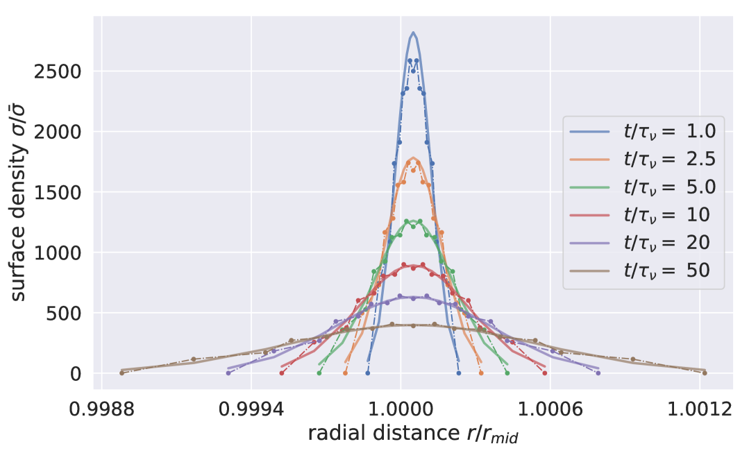
Figure 24: Radial spreading of a initially narrow circular viscous non-gravitating ringlet, simulation (dashed curves with dots) versus theory (solid curves). The simulated ringlet has the same physical properties as the nominal ringlet: total mass $m_{r}=10^{-10}$, initial semimajor axis width $\Delta a_{0}=10^{-4}$, shear viscosity $\nu_{s}=10^{-13}$, and bulk viscosity $\nu_{b}=\nu_{s}$. However this simulated ringlet is composed of $N_{s}=13$ streamlines instead of two, and all streamlines are initially circular, $e=0$. And because a circular ringlet is always axisymmetric only $N_{p}=3$ particles per streamline need be used here. Each colored curve indicates the ringlet’s radial surface density profile $\sigma(r)/\bar{\sigma}$ versus radial distance $r/r_{mid}$ at various times $t/\tau_{\nu}$, where $\tau_{\nu}$ is the viscous timescale and $r_{mid}$ is the radius of the ringlet’s middle. Solid theoretical curves are from Eqn. (2.13) of Pringle (1981) where the constant $\bar{\sigma}=m_{r}/\pi r_{mid}^{2}$.

C.0.2 self gravitating ringlets

Borderies et al. (1983b) show that a gravitating ringlet has an equilibrium eccentricity difference $\Delta e^{0}=e_{\text{outer}}-e_{\text{inner}}$ that is stationary. Which means that if a ringlet is in equilibrium, it will precess as rigid body with its streamlines experiencing zero relative motions and with steady $\Delta e$ over time. Multiplying their expression for the equilibrium $\Delta e^{0}$ by $a/\Delta a$ then provides the ringlet’s equilibrium dimensionless eccentricity gradient:

$$e^{\prime}_{eq}=a\frac{\Delta e^{0}}{\Delta a}=\frac{21\pi eJ_{2}}{4H(q)}\left(\frac{M}{m_{r}}\right)\left(\frac{R_{p}}{a}\right)^{2}\left(\frac{\Delta a}{a}\right)^{2}$$ (C1)

where the nonlinearity parameter $q=|e^{\prime}|$ since $\tilde{\omega}^{\prime}=0$ for an inviscid ringlet in equilibrium, and the function

$$H(q)=\frac{1-\sqrt{1-q^{2}}}{q^{2}\sqrt{1-q^{2}}}.$$ (C2)

Borderies et al. (1983b) also show that when the ringlet is displaced slightly from equilibrium, $e^{\prime}$ will librate about the equilibrium point, Eqn (C1). Which makes it straightforward to iteratively determine a ringlet’s equilibrium $e^{\prime}_{eq}$ numerically via a handful of short epi_int_lite simulations, the results of which are summarized in Fig. 25 which compares simulated ringlet equilibria (dots) with theory (continuous curves) for a variety of inviscid gravitating ringlets. That Figure shows that the agreement between the epi_int_lite simulations and theoretical expectations, Eqn. (C1), is overall very good, though modest discrepancies do exist for the higher-mass ringlets whose equilibrium $e^{\prime}_{eq}$ are small.

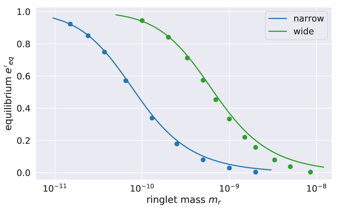
Figure 25: Equilibrium $e^{\prime}_{eq}$ for two kinds of inviscid $\nu=0$ gravitating ringlets. Blue curve is for narrower lower-mass ringlets that all have the same semimajor axis width $\Delta a=5\times 10^{-4}$, eccentricity $e=0.0025$, and the indicated range of ringlet masses $m_{r}$. Green curve is for wider higher-mass ringlets whose $\Delta a$ and $e$ are larger by $\times 2$. Dots indicate outcomes from epi_int_lite simulations while continuous curves are the theoretical predictions from Borderies et al. (1983b).

And when a ringlet is displaced slightly from equilibrium, it will librate about the equilibrium point (C1) with angular frequency $\Omega_{\text{lib}}$ given by Eqn. (30) of Borderies et al. (1983b). So a ringlet’s libration period is

$$T_{\text{lib}}=\frac{2\pi}{\Omega_{\text{lib}}}=\frac{\pi}{H(q)}\left(\frac{M}{m_{r}}\right)\left(\frac{\Delta a}{a}\right)^{2}T_{\text{orb}}$$ (C3)

where $T_{\text{orb}}$ is the ringlet’s orbital period, which is shown in Fig. 26 for the simulated ringlets of Fig 25. That Figure compares predicted libration periods (dashed curves) versus simulated $T_{\text{lib}}$ (dotted curves) for the suite of narrow and wide ringlets. The rightmost portions of the blue and green curves show that the higher-mass simulated ringlets’ have libration periods $T_{\text{lib}}$ that are in excellent agreement with theory, Eqn. (C3). However significant disagreement exists in the leftmost portions of these curves, which corresponds to the lower-mass narrow & wide ringlets. This disagreement is a consequence of the simulated ringlets’ evolution violating a key assumption of the Borderies et al. (1983b) derivation: that the ringlet’s libration amplitude $A$ and its libration frequency $\Omega_{\text{lib}}$ are constant during a libration cycle. In all of the simulations reported on in Fig. 26, the ringlet’s libration amplitude and frequency do vary over time, but those simulations show the their fractional variations $\Delta A/A$ and $\Delta\Omega_{\text{lib}}/\Omega_{\text{lib}}$ are progressively smaller in the higher-mass ringlets. For instance the three lowest-mass blue and green simulations in Fig. 26 have $\Delta A/A>0.5$ while that quantity is significantly smaller for the higher-mass ringlets. From this we conclude that the lower-mass simulations are exploring parameter space where the theoretical predictions do not apply. And that the higher-mass simulations are in excellent agreement with theory.

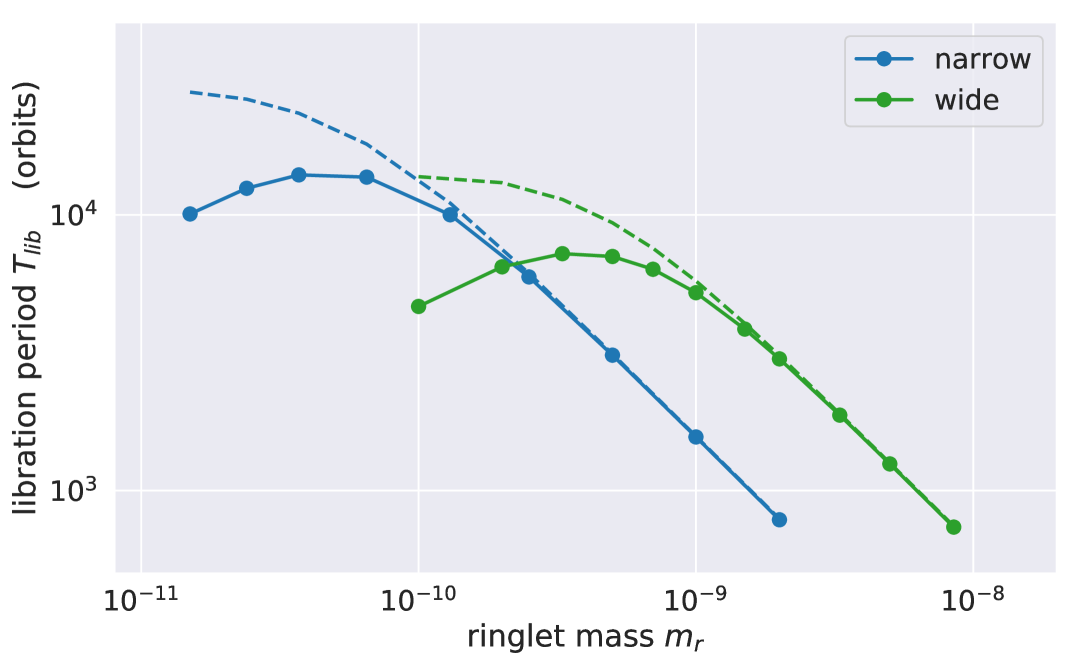
Figure 26: Libration period $T_{\text{lib}}$ versus ringlet mass $m_{r}$ for the suite of narrow and wide ringlets also simulated in Fig. 25. Dotted curves are the simulated outcomes while dashed curves are from Eqn. (C3) derived in (Borderies et al., 1983b). Note that outcomes for the lower-mass ringlet simulations do disagree with theory, but they are exploring a parameter space where the assumptions utilized in the derivation do not apply.

Appendix D Appendix D

This examines the viscous evolution of a narrow eccentric non-gravitating ringlet that is identical to the nominal ringlet of Section 3.1 but with ringlet self-gravity neglected and $J_{2}=0$. As the orange curve in Fig. 27 shows, the non-gravitating ringlet’s radial width $\Delta a$ grows over time due to ringlet viscosity, long after the nominal self-gravitating ringlet (blue curve) has settled into the self-confining state by time $t\sim 40\tau_{\nu}$. This is due to the ringlet’s secular gravitational perturbations of itself, which tends to excites the ringlet’s outer streamline’s eccentricity at the expense of the inner streamline (see Fig. 3) until the ringlet eccentricity gradient $e^{\prime}$ (blue curve in Fig. 28) grows beyond the limit required for complete angular momentum flux reversal that results in the ringlet’s radial confinement (dotted line). Note that viscosity also excites the non-gravitating ringlet’s eccentricity gradient some (orange curve), but not sufficiently to halt the ringlet’s viscous spreading.

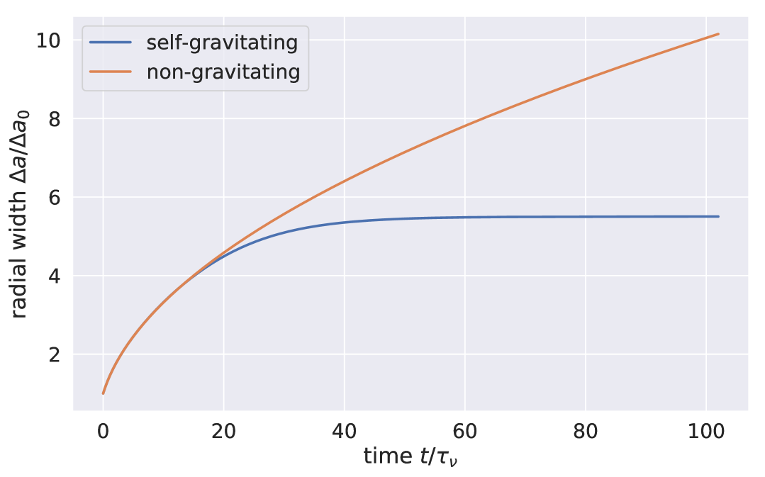
Figure 27: Blue curve is the nominal ringlet’s semimajor axis width $\Delta a$ versus time $t$, and this ringlet’s radial spreading ceases by time $t\sim 40\tau_{\nu}$ when it’s self-gravity has excited the ringlet’s eccentricity gradient $e^{\prime}$ sufficiently; see blue curve in Fig. 28. Orange curve shows that the non-gravitating ringlet’s $\Delta a$ grows without limit due to the ringlet’s much lower eccentricity gradient. Note that planetary oblateness would cause the non-gravitating streamlines to precess differentially and eventually cross when $J_{2}>0$, so the non-gravitating simulation also sets $J_{2}=0$ to avoid differential precession.

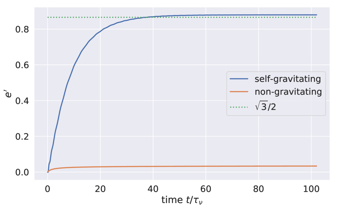
Figure 28: Eccentricity gradient $e^{\prime}$ versus time $t$ for self-gravitating nominal ringlet (blue curve), and non-gravitating ringlet (orange).

References

- Borderies et al. (1982) Borderies, N., Goldreich, P., & Tremaine, S. 1982, Nature, 299, 209
- Borderies et al. (1983a) —. 1983a, Icarus, 55, 124
- Borderies et al. (1983b) —. 1983b, AJ, 88, 1560
- Borderies et al. (1985) —. 1985, Icarus, 63, 406
- Borderies et al. (1986) —. 1986, Icarus, 68, 522
- Borderies-Rappaport & Longaretti (1994) Borderies-Rappaport, N., & Longaretti, P.-Y. 1994, Icarus, 107, 129
- Brouwer & Clemence (1961) Brouwer, D., & Clemence, G. M. 1961, Methods of celestial mechanics (New York: Academic Press, 1961)
- Chambers (1999) Chambers, J. E. 1999, MNRAS, 304, 793
- Charnoz et al. (2010) Charnoz, S., Salmon, J., & Crida, A. 2010, Nature, 465, 752
- Chiang & Goldreich (2000) Chiang, E. I., & Goldreich, P. 2000, ApJ, 540, 1084
- French et al. (2024) French, R. G., Hedman, M. M., Nicholson, P. D., Longaretti, P.-Y., & McGhee-French, C. A. 2024, Icarus, 411, 115957
- French et al. (2016a) French, R. G., Nicholson, P. D., Hedman, M. M., et al. 2016a, Icarus, 279, 62
- French et al. (2016b) French, R. G., Nicholson, P. D., McGhee-French, C. A., et al. 2016b, Icarus, 274, 131
- Goldreich et al. (1995) Goldreich, P., Rappaport, N., & Sicardy, B. 1995, Icarus, 118, 414
- Goldreich & Tremaine (1979a) Goldreich, P., & Tremaine, S. 1979a, AJ, 84, 1638
- Goldreich & Tremaine (1979b) —. 1979b, Nature, 277, 97
- Goldreich & Tremaine (1981) —. 1981, ApJ, 243, 1062
- Goldreich & Tremaine (1982) —. 1982, ARA&A, 20, 249
- Hahn (2009) Hahn, J. M. 2009, in AAS/Division of Dynamical Astronomy Meeting, Vol. 40, AAS/Division of Dynamical Astronomy Meeting, #06.12–+
- Hahn & Spitale (2013) Hahn, J. M., & Spitale, J. N. 2013, ApJ, 772, 122
- Jones et al. (2023) Jones, J. W., Chiang, E., Duchêne, G., Kalas, P., & Esposito, T. M. 2023, ApJ, 948, 102
- Longaretti (2018) Longaretti, P. Y. 2018, Theory of Narrow Rings and Sharp Edges (Cambridge University Press), 225–275
- Matthews et al. (2018) Matthews, B., Greaves, J., Kennedy, G., et al. 2018, in Astronomical Society of the Pacific Conference Series, Vol. 517, Science with a Next Generation Very Large Array, ed. E. Murphy, 161
- Mosqueira & Estrada (2002) Mosqueira, I., & Estrada, P. R. 2002, Icarus, 158, 545
- Murray et al. (2005) Murray, C. D., Chavez, C., Beurle, K., et al. 2005, Nature, 437, 1326
- Nicholson et al. (2014) Nicholson, P. D., French, R. G., McGhee-French, C. A., et al. 2014, Icarus, 241, 373
- Poulet & Sicardy (2001) Poulet, F., & Sicardy, B. 2001, MNRAS, 322, 343
- Pringle (1981) Pringle, J. E. 1981, ARA&A, 19, 137
- Rimlinger et al. (2016) Rimlinger, T., Hamilton, D., & Hahn, J. M. 2016, in AAS/Division of Dynamical Astronomy Meeting, Vol. 47, AAS/Division of Dynamical Astronomy Meeting, #47, id.400.02
- Shu (1984) Shu, F. H. 1984, in IAU Colloq. 75: Planetary Rings, ed. R. Greenberg & A. Brahic, 513–561
- Shu et al. (1985) Shu, F. H., Yuan, C., & Lissauer, J. J. 1985, ApJ, 291, 356
- Spitale & Hahn (2016) Spitale, J. N., & Hahn, J. M. 2016, Icarus, 279, 141
- Strubbe & Chiang (2006) Strubbe, L. E., & Chiang, E. I. 2006, ApJ, 648, 652
- Tiscareno et al. (2010) Tiscareno, M. S., Burns, J. A., Sremčević, M., et al. 2010, ApJ, 718, L92
- Weiss et al. (2009) Weiss, J. W., Porco, C. C., & Tiscareno, M. S. 2009, AJ, 138, 272