Boson stars in the $U(1)$ gauged 3+1 dimensional $O(3)$ sigma-model

Abstract

We study regular self-gravitating non-topological soliton solutions of the $U(1)$ gauged non-linear $O(3)$ sigma model with the usual kinetic term and a simple symmetry breaking potential in 3+1 dimensional asymptotically flat spacetime. Both parity-even and parity-odd configurations with an angular node of the scalar field are considered. Localized solutions are endowed with an electric charge, spinning configurations are also coupled to the toroidal flux of magnetic field. We confirm that such solutions do not exist in the flat space limit. Similar to the usual boson stars, a spiral-like frequency dependence of the mass and the Noether charge of the gauged solutions is observed. Depending on the relative strength of gravity and the electromagnetic interaction, the resulting gauged $O(3)$ boson stars at the mass threshold either possess the usual Newtonian limit, or they are linked to a regular strongly gravitating critical configuration. We explore domain of existence of the solutions and investigate some of their physical properties.

I Introduction

It has been known for a long time that matter fields can be localized by gravity Wheeler:1955zz , see e.g. Jetzer:1991jr ; Schunck:2003kk ; Liebling:2012fv ; Shnir:2022lba for detailed review. So-called boson stars Kaup:1968zz ; Feinblum:1968nwc ; Ruffini:1969qy ; Colpi:1986ye , which represent localized configurations of a self-gravitating oscillating complex scalar field with a harmonic phase, provide a simple example of such configurations. Boson stars have attracted increasing attention in the last decade, in particular as black hole mimickers Guzman:2009zz ; Torres:2000dw ; Olivares:2018abq and modeling of galactic halos and their lensing properties Mielke:2002bp ; Schunck:2006rk ; Chen:2020cef . Further, the boson stars are considered as possible candidates for the hypothetical weakly-interacting ultralight component of dark matter Preskill:1982cy ; Dine:1982ah ; Guth:2014hsa ; Matos:1998vk ; Suarez:2013iw ; Levkov:2016rkk .

In the simplest case, boson stars arise as solutions of the Einstein-Klein-Gordon theory with a massive complex scalar field coupled to gravity without self-interaction. These mini-boson stars do not have a regular flat spacetime limit. Very large massive boson stars exist in the models with polynomial potentials Kleihaus:2005me ; Kleihaus:2007vk or in the two-component Einstein-Friedberg-Lee-Sirlin model Friedberg:1986tq . They are linked to the corresponding flat space configurations, which represent stable isospinning non-topological solitons, the Q-balls Rosen:1968mfz ; Friedberg:1976me ; Coleman:1985ki .

Isorotations may also stabilise self-gravitating non-topological solitons in the non-linear $O(3)$ sigma model with a non-negative potential Verbin:2007fa ; Cano:2023bpe ; Adam:2025ktm . There are families of regular asymptotically flat stationary spinning $O(3)$ sigma model solutions, and hairy black holes in a simple model which include only the usual kinetic term and a symmetry breaking potential Verbin:2007fa ; Herdeiro:2018djx ; Cano:2023bpe . Dynamical evolutions of such solutions closely resemble the pattern found for the spinning complex scalar fields coupled to gravity, the boson stars and black holes with synchronised hair Kaup:1968zz ; Feinblum:1968nwc ; Ruffini:1969qy ; Colpi:1986ye ; Hod:2012px ; Herdeiro:2014goa . These non-topological stationary solutions of the $O(3)$ non-linear sigma model minimally coupled to gravity trivialize in the flat space limit Verbin:2007fa ; Herdeiro:2018djx . Indeed, in 3+1 dimensions, the Derrick’s theorem Derrick:1964ww does not allow for the existence of such static finite energy solitons in the usual $O(3)$ sigma model, which includes only quadratic in derivative term and a potential. Such topological solitons, referred as Hopfions, appear in the scale-invariant Nicole model Nicole:1978nu and, more importantly, in the Faddeev-Skyrme model Faddeev:1976pg , which contains terms with both two and four derivatives. Apart the addition of higher derivative terms, no other mechanism to secure stability of the regular topological solitons of the $O(3)$ sigma model in three spacial dimensions is known.

Self-gravitating Hopfions in the $O(3)$ Faddeev-Skyrme model are smoothly connected to the corresponding flat space topological solitons of certain degrees Shnir:2015lli . However, the virial theorem does not exclude existence of regular isospinning $O(3)$ solitons stabilized by internal rotation in the flat space Herdeiro:2018djx , certain modification of the potential term may allow for construction of such non-topological solitons in 3+1 dimensional space.

As it turns out, the boson stars posses a complicated morphology Friedberg:1986tq ; Yoshida:1997nd ; Kleihaus:2007vk ; Herdeiro:2019mbz ; Cunha:2022tvk ; Shnir:2022lba ; Liang:2025myf . In the simplest case, these solutions are spherically symmetric, also there are axially symmetric boson stars with a non-zero angular momentum, solutions with negative parity, radially excited boson stars and a variety of non-trivial multipolar stationary configurations without any continuous symmetries. Qualitatively, the appearance of such solutions may be related to the force balance between the repulsive scalar interaction and the gravitational attraction in equilibria. Furthermore, the local $U(1)$ symmetry of a model supporting Q-balls can be promoted to the local gauge symmetry, corresponding gauged Q-balls possess electric charge Rosen:1968mfz ; Lee:1988ag ; Anagnostopoulos:2001dh ; Gulamov:2013cra ; Gulamov:2015fya . The presence of the long-range gauge field affects the properties of the solitons, as the gauge coupling increases, the electromagnetic repulsion may destroy configurations. Gravitational attraction, on the other hand, may produce an opposite effect, the pattern of dynamical evolution of gauged boson stars can be rather complicated Kunz:2021mbm .

The objective of this paper is to analyze the properties of the regular self-gravitating solutions of the $U(1)$ gauged non-linear $O(3)$ sigma model minimally coupled to Einstein gravity, focusing our study on non-topological localized configurations of different types, and determine their domains of existence.

This paper is organized as follows. In Section II, we introduce the model, and the field equations with the stress-energy tensor of the system of interacting fields. Here we describe the axially-symmetric parametrization of the metric and the matter fields and the boundary conditions imposed on the configuration. We also discuss the physical quantities of interest.

In Sec. III we present the results of our study of self-gravitating solitons with particular emphasis on the role of the electromagnetic interaction. We conclude with a discussion of the results and final remarks.

II The model

II.1 The action and the field equations

We consider the $U(1)$ gauged non-linear sigma-model, which is minimally coupled to Einstein’s gravity in a (3+1)-dimensional space-time. The corresponding action of the system is

$$S=\int d^{4}x\sqrt{-{\mathcal{g}}}\left(\frac{R}{16\pi G}-L_{m}\right),$$ (1)

where the rescaled matter field Lagrangian is

$$L_{m}=-\frac{1}{4}F_{\mu\nu}F^{\mu\nu}+\frac{1}{2}(D_{\mu}\phi^{a})^{2}+U(\phi)\,.$$ (2)

Here $R$ is the Ricci scalar associated with the spacetime metric $g_{\mu\nu}$ with the determinant ${\mathcal{g}}$ and $G$ is the Newton’s constant. In the matter field Lagrangian the real triplet of the scalar fields $\phi^{a}$, $a=1,2,3$, is restricted to the surface of the unit sphere, $(\phi^{a})^{2}=1$ and the symmetry breaking potential is

$$U(\phi)=\mu^{2}(1-\phi^{3})\,,$$ (3)

where a mass parameter $\mu$ is a constant.

Such potential breaks $O(3)$ symmetry to the subgroup $SO(2)$, and the corresponding Noether current can be written as follows:

$$j^{\mu}=-\phi^{1}D^{\mu}\phi^{2}+\phi^{2}D^{\mu}\phi^{1}$$ (4)

The $U(1)$ field strength tensor is $F_{\mu\nu}=\partial_{\mu}A_{\nu}-\partial_{\nu}A_{\mu}$, and the covariant derivative of the field $\phi^{a}$, that minimally couples the scalar field to the gauge potential is

$$D_{\mu}\phi^{\alpha}=\partial_{\mu}\phi^{\alpha}+e\,A_{\mu}\,\varepsilon_{\alpha\beta}\,\phi^{\beta}\,,\qquad D_{\mu}\phi^{3}=\partial_{\mu}\phi^{3},\qquad\alpha,\,\beta=1,\,2\,$$ (5)

with the gauge coupling $e$. The vacuum boundary conditions are $\phi_{\infty}^{a}=(0,0,1),\,D_{\mu}\phi^{a}=0,\,F_{\mu\nu}=0$. In the static gauge, where the fields have no explicit dependence on time, the asymptotic boundary conditions on the gauge potential are

$$A_{0}(\infty)=V,\quad A_{i}(\infty)=0$$ (6)

where $V$ is a real constant. The model (2) is invariant with respect to the local Abelian gauge transformations

$$(\phi^{1}+i\phi^{2})\to e^{ie\zeta}(\phi^{1}+i\phi^{2}),\quad A_{\mu}\to A_{\mu}-\partial_{\mu}\zeta$$ (7)

where $\zeta$ is a real function of the coordinates. We remark that asymptotic value of the electric potential $A_{0}(\infty)$ can be adjusted via the residual $U(1)$ transformations, choosing $\zeta=-Vt$. In the stationary gauge $A_{0}(\infty)=0$ and two components (7) of the scalar triplet acquire an explicit harmonic time dependence with frequency $\omega=eV$.

Variation of the action (1) with respect to metric yields the Einstein equations:

$$R_{\mu\nu}-\frac{1}{2}Rg_{\mu\nu}=2\alpha^{2}\left(T_{\mu\nu}^{Em}+T_{\mu\nu}^{\phi}\right)$$ (8)

where $\alpha^{2}=16\pi G$ is the effective gravitational coupling and the electromagnetic and scalar components of the energy-momentum tensor are

$$\begin{split}T_{\mu\nu}^{Em}&=F_{\mu}^{\rho}F_{\nu\rho}-\frac{1}{4}g_{\mu\nu}F_{\rho\sigma}F^{\rho\sigma}\,,\\ T_{\mu\nu}^{\phi}&=D_{\mu}\phi^{a}D_{\nu}\phi^{a}-g_{\mu\nu}\left[\frac{g^{\rho\sigma}}{2}D_{\rho}\phi^{a}D_{\sigma}\phi^{a}+U(\phi)\right]\,.\end{split}$$ (9)

We notice that the sigma model constraint does not allow us to absorb the mass parameter $\mu$ into the scaled expression for the scalar field.

We obtain field equations by variation of the action (1) with the respect to the field $A_{\mu}$ and $\phi_{a}$:

$$\partial_{\mu}\left(\sqrt{-{\mathcal{g}}}F^{\mu\nu}\right)=e\sqrt{-{\mathcal{g}}}j^{\nu},\quad D^{\mu}D_{\mu}\phi^{a}+\phi^{a}(D^{\mu}\phi^{b}\cdot D_{\mu}\phi^{b})+\mu^{2}\left[\phi^{a}(\phi^{b}\cdot\phi^{b}_{\infty})-\phi^{a}_{\infty}\right]=0\,,$$ (10)

where we take into account dynamical constraint imposed on the $O(3)$ field.

The asymptotic expansion of the fields around the vacuum

$$\phi^{a}\approx\phi^{a}_{\infty}+\delta\phi^{a},\qquad A_{\mu}\approx a_{\mu}+\delta_{0\mu}(eV-\omega)$$ (11)

where $\delta\phi^{a}=(1-v_{0},\,v_{1},\,v_{2})$, gives the effective stationary Lagrangian of linearized scalar excitations

$$L_{pert}=\frac{1}{2}(\partial_{i}v_{\alpha})^{2}+\mu^{2}v_{\alpha}^{2}-(eV-\omega)^{2}v_{\alpha}^{2}$$ (12)

Here $\alpha=1,2$ and we take into account the residual gauge invariance of the system. Note that the fluctuations of the component $v_{0}$ correspond to the second order of the expansion around the vacuum. Hence, the squared effective mass of the scalar excitations $v_{\alpha}$ is $m_{eff}^{2}=\mu^{2}-(eV-\omega)^{2}$ and localized massive scalar modes with exponentially decaying tail may exist if $m_{eff}^{2}$ is positive. In the stationary gauge $V=0$ and the self-gravitating non-topological $O(3)$ solitons may occur within a restricted interval of values of the angular frequency $\omega\in[\omega_{min},\mu].$ The configurations smoothly approach perturbations around Minkowski spacetime and delocalize as $\omega\to\mu$. This is usually referred to as the Newtonian limit.

II.2 Self-gravitating solitons: The ansatz

We are interested in stationary axially-symmetric regular localized solutions of the system of equations (8) and (10), which are similar to the usual boson stars. We adopt the isotropic Lewis-Papapetrou-type metric in adapted “quasi-isotropic” spherical coordinates $(t;r;\theta;\varphi)$, for which the line element reads

$$ds^{2}=-e^{f_{0}(r,\theta)}dt^{2}+e^{f_{1}(r,\theta)}(dr^{2}+r^{2}d\theta^{2})+e^{f_{2}(r,\theta)}r^{2}\sin^{2}{\theta}(d\varphi-\frac{W(r,\theta)}{r}dt)^{2}\,.$$ (13)

The Minkowski spacetime asymptotic is approached for $r\to\infty$ with $f_{0}=f_{1}=f_{2}=W=0$. Spherically symmetric solutions correspond to the reduction $W(r,\theta)=0$, $f_{1}(r)=f_{2}(r)$, both metric functions $f_{0}$ and $f_{1}$ then depend on the isotropic radial coordinate $r$ only.

For the scalar $O(3)$ field, we adopt a stationary ansatz with a harmonic time dependence, which is similar to the corresponding parametrization of the $O(4)$ Skyrme model Battye:2014qva ; Ioannidou:2006nn ; Perapechka:2017bsb ; Herdeiro:2018daq and the $U(1)$ gauged Skyrmions Kirichenkov:2023omy ; Livramento:2023keg ; Livramento:2023tmm ,

$$\phi^{a}=[\sin{f(r,\theta)}\cos{(n\varphi-\omega t)},\text{ }\sin{f(r,\theta)}\sin{(n\varphi-\omega t)},\text{ }\cos{f(r,\theta)}].$$ (14)

The Ansatz for the $U(1)$ potential contains two real functions – an electric and a magnetic potential:

$$A_{\mu}dx^{\mu}=A_{t}(r,\theta)dt+A_{\varphi}(r,\theta)\sin{\theta}d\varphi$$ (15)

Recall that in the stationary gauge $A_{t}=A_{\varphi}=0$ at spacial infinity.

The $U(1)$ gauged charged self-gravitating solutions are characterized by a set of physical observables, the Arnowitt-Deser-Misner (ADM) mass $M$, the angular momentum $J$, the electric charge $Q_{e}$ and the dipole moment $\mu_{m}$. These quantities can be extracted from the asymptotic behaviour of the metric and the gauge field functions, as

$$\begin{split}g_{tt}&\rightarrow-1+\frac{\alpha^{2}M}{\pi r}+O(\frac{1}{r^{2}}),\quad g_{t\phi}\rightarrow-\frac{\alpha^{2}J}{\pi r}\sin^{2}{\theta}+O(\frac{1}{r^{2}})\\ A_{t}&\rightarrow\frac{Q_{e}}{r}+O(\frac{1}{r^{2}}),\quad A_{\varphi}\rightarrow\frac{\mu_{m}\sin^{2}\theta}{r^{2}}+O(\frac{1}{r^{3}})\end{split}$$ (16)

The ADM mass and the total angular momentum can also be computed as the Komar integrals of the corresponding densities of the total stress-energy tensor $T_{\mu\nu}=T^{\phi}_{\mu\nu}+T^{Em}_{\mu\nu}$,

$$M=\int\sqrt{-\mathcal{g}}drd\theta d\varphi\left(T^{\mu}_{\mu}-2T^{t}_{t}\right),\quad J=\int\sqrt{-\mathcal{g}}drd\theta d\varphi T^{t}_{\varphi}$$ (17)

In other words, the mass $M$ and the angular momentum $J$ are conserved charges associated with the two Killing vectors, $\partial_{t}$ and $\partial_{\varphi}$, respectively.

The temporal component of the current density (4) yields the Noether charge

$$Q=\int\sqrt{-\mathcal{g}}drd\theta d\varphi~j^{0}=2\pi\int_{0}^{\infty}dr\int_{0}^{\pi}d\theta\sin^{2}{f}\left(\omega-\frac{nW}{r}\right)e^{f_{1}+\frac{1}{2}f_{2}-\frac{1}{2}f_{0}}r^{2}\sin{\theta}.$$ (18)

where we make use of the parametrization of the metric (13) and the $O(3)$ field (14). One can show that $J$, $Q$ and the electric charge $Q_{e}$ are proportional, see e.g. ref. Schunck:1996he ; Collodel:2019ohy ; Herdeiro:2021jgc :

$$J=nQ=\frac{nQ_{e}}{e}$$ (19)

where $n$ is the winding number of the scalar field. We also note that we consider regular self-gravitating configurations with zero entropy and without an intrinsic temperature. However, they obey the truncated first law of thermodynamics without the entropy term: $dM=\omega dQ$, see e.g. Herdeiro:2021mol ; Stotyn:2013spa .

Substitution of the ansatz (13),(14) and (15) into general field equations (8), (10) reduces them to a system of seven coupled nonlinear partial differential equations in $r$ and $\theta$. In order to find asymptotically flat and regular solutions, appropriate boundary conditions need to be imposed. The assumption of asymptotic flatness at the spacial infinity with our choice of the stationary gauge for the Maxwell potentials, gives

$$f|_{r\rightarrow{\infty}}=f_{0}|_{r\rightarrow{\infty}}=f_{1}|_{r\rightarrow{\infty}}=f_{2}|_{r\rightarrow{\infty}}=W|_{r\rightarrow{\infty}}=A_{t}|_{r\rightarrow{\infty}}=A_{\varphi}|_{r\rightarrow{\infty}}=0$$ (20)

On the symmetry axis, the regularity and the axial symmetry implies the following conditions ($n\neq 0$)

$$\begin{split}\partial_{\theta}W|_{\theta=0,\pi}=\partial_{\theta}f_{0}|_{\theta=0,\pi}=\partial_{\theta}f_{1}|_{\theta=0,\pi}=\partial_{\theta}f_{2}|_{\theta=0,\pi}=0\,,\\ f|_{\theta=0,\pi}=\partial_{\theta}A_{\varphi}|_{\theta=0,\pi}=\partial_{\theta}A_{t}|_{\theta=0,\pi}=0\,.\end{split}$$ (21)

For the spherically symmetric configuration ($n=0$) we impose $\partial_{\theta}f|_{\theta=0,\pi}=0$.

Further, the condition of the absence of a conical singularity at the symmetry axis requires that the deficit angle should vanish, $\delta=2\pi\left(1-\lim_{\theta\to 0}\frac{f_{2}}{f_{1}}\right)=0$. Therefore, the solutions should satisfy the constrain $f_{1}|_{\theta=0,\pi}=f_{2}|_{\theta=0,\pi}=0$, see Herdeiro:2018djx ; Herdeiro:2021mol . In our numerical scheme we explicitly imposed this condition.

We assume the solutions are $\mathbb{Z}_{2}$-symmetric under reflections with respect to the equatorial plane. Thus, there are two different types of axially symmetric regular solutions, which possess different parity Kleihaus:2005me ; Kleihaus:2007vk . For a system with even parity ($\mathcal{P}=1$), all angular derivatives must vanish on the equatorial plane

$$\begin{split}\partial_{\theta}W|_{\theta=\frac{\pi}{2}}=\partial_{\theta}f_{0}|_{\theta=\frac{\pi}{2}}=\partial_{\theta}f_{1}|_{\theta=\frac{\pi}{2}}=0\,,\\ \partial_{\theta}f_{2}|_{\theta=\frac{\pi}{2}}=\partial_{\theta}A_{\varphi}|_{\theta=\frac{\pi}{2}}=\partial_{\theta}A_{t}|_{\theta=\frac{\pi}{2}}=0\,.\end{split}$$ (22)

and $\partial_{\theta}f|_{\theta=\frac{\pi}{2}}=0$. For the parity-odd ($\mathcal{P}=-1$) solutions the boundary condition on the $O(3)$ field is different, $f|_{\theta=\frac{\pi}{2}}=0$.

Finally, regularity of the solutions at the origin requires that both for the parity-even and parity-odd axially-symmetric configurations ($n\neq 0$) we impose

$$\begin{split}f|_{r=0}=W|_{r=0}=\partial_{r}f_{0}|_{r=0}=\partial_{r}f_{1}|_{r=0}=0\,,\\ \partial_{r}f_{2}|_{r=0}=A_{\varphi}|_{r=0}=\partial_{r}A_{t}|_{r=0}=0\,.\end{split}$$ (23)

For the spherically symmetric solution ($n=0$) the boundary condition on the scalar field is different, $\partial_{r}f|_{r=0}=0$.

III Results

III.1 Numerical approach

We have solved the boundary value problem subject to the boundary conditions (20)-(23) above with a forth-order finite difference scheme, where the system of seven differential equations is discretized on a grid with a typical size of $200\times 30$ points. In our numerical calculations we introduce a new compact radial coordinate

$$x=\frac{r}{c+r}\,,$$ (24)

which maps the semi-infinite region $[0;\infty)$ onto the unit interval $[0;1]$. Here $c$ is an arbitrary constant which is used to adjust the contraction of the grid. In our calculations, we typically take $c\in[0.1,20]$.

The corresponding system of nonlinear algebraic equations has been solved using the Newton-Raphson scheme with the Intel MKL PARDISO sparse direct solver MKL . Calculations have been performed with the package equipped with an adaptive mesh selection procedure, and the CESDSOL library. Typical errors are of order of $10^{-8}$. The solutions do not exhibit conical singularities at the level of numerical accuracy, numerical calculations confirm that both the Ricci and the Kretschmann scalars are finite.

The morphology of so constructed solutions can be very complicated Kleihaus:2005me ; Kleihaus:2007vk ; Yoshida:1997nd ; Herdeiro:2021mol ; Herdeiro:2020kvf . In Fig. 1 we displayed, as an example, four different types of the gravitating soliton solutions of the $O(3)$ sigma model to be discussed below. The parity-even configurations possess spherical or axial symmetry while the parity-odd solutions represent multi-nodal configurations which are symmetrically aligned along the symmetry axis.

III.2 Spherical solutions

Assuming the spherical symmetry ($n=0$), the system of field equations (8), (10) is reduced to the system of four coupled ordinary differential equations of functions $f,f_{0},f_{1}$ and $A_{t}$ are functions of $r$ only. Further, in such a case we can employ Schwarzschild-like coordinates, with a line element

$$ds^{2}=-N(r)\sigma^{2}(r)dt^{2}+\frac{1}{N(r)}dr^{2}+r^{2}(d\theta^{2}+\sin^{2}\theta d\varphi^{2})$$ (25)

where $N(r)=1-\frac{2m(r)}{r}$. The ADM mass of the solution is determined by the asymptotic value of the mass function $m(\infty)$.

With this parametrization the reduced curvature scalar is

$$R=-2\sigma(N-1-rN^{\prime})$$

and problem reduces to solving two second order equation for the scalar profile function $f$ and electric potential $A_{t}$ (in the static gauge), and two first order equations for the metric functions $m$ and $\sigma$:

$$(r^{2}N\sigma f^{\prime})^{\prime}=r^{2}\sigma\left(\mu^{2}-\frac{e^{2}A_{t}^{2}}{N\sigma^{2}}\cos{f}\right)\sin{f},$$ (26)

$$m^{\prime}=\frac{\alpha^{2}r^{2}}{8}\left(Nf^{\prime 2}+4\mu^{2}\sin^{2}{\left(\frac{f}{2}\right)}+\frac{e^{2}A_{t}^{2}}{N\sigma^{2}}-\frac{A_{t}^{\prime 2}}{\sigma^{2}}\right),$$ (27)

$$\sigma^{\prime}=\frac{\alpha^{2}r\sigma}{4}\left(f^{\prime 2}+\frac{e^{2}A_{t}^{2}}{N^{2}\sigma^{2}}\sin^{2}{f}\right),$$ (28)

$$(r^{2}\sigma A_{t}^{\prime})^{\prime}=2r^{2}A_{t}^{\prime}\sigma^{\prime}-\frac{er^{2}A_{t}}{N}\sin^{2}{f}.$$ (29)

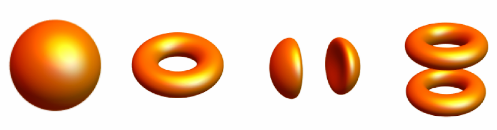
Figure 1: Illustrative examples of different types of solitonic solutions of the $O(3)$ sigma model. The surfaces of constant charge density for fundamental spherically symmetric solution, axially symmetric $n=1$ solution, dipole $n=0$ solution and parity-odd $n=1$ solution, from left to right, respectively, are plotted for gravitational coupling $\alpha^{2}=1$, frequency $\omega=0.85$, and gauge coupling $e=0.2$.

The system of equation (26)-(29) can be solved numerically subject to the boundary conditions

$$\begin{split}N|_{r=0}&=1,\quad\partial_{r}A_{t}|_{r=0}=\partial_{r}\sigma|_{r=0}=\partial_{r}f|_{r=0}=0,\\ N|_{r=\infty}&=1,\quad A_{t}|_{r=\infty}=0,~~\sigma|_{r=\infty}=1,~~f|_{r=\infty}=0\end{split}$$ (30)

The Schwarzschild-like parametrization is useful to analyze possible formation of the event horizon and asymptotic behavior of the solutions, cf. corresponding equations for regular ungauged self-gravitating solutions of the $O(3)$-sigma model Herdeiro:2018djx . On the other hand, it also can be studied in isotropic coordinates, which is more convenient for our purposes, comparing various solutions with spherical and axial symmetry.

First, we can choose $\alpha^{2}=1$, $\mu^{2}=1$ and make use of the the time dependent gauge. This allows us to compare our results with those obtained in Herdeiro:2018djx for ungauged gravitating $O(3)$ solutions. There are two continuous input parameters, the frequency $\omega$, the gauge coupling $e$ and one discrete parameter $n$.

The spherically symmetric solutions are fundamental states, for which the matter fields profiles possess no nodes both in radial and angular directions. As the gauge coupling $e$ is set to be zero, regular gravitating boson-star-like solutions of the non-linear $O(3)$ sigma model are recovered Herdeiro:2018djx . A family of charged solutions emerge from the uncharged regular boson-star-like solutions when the parameter $e$ is gradually increased from zero while the other input parameters remain fixed.

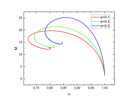
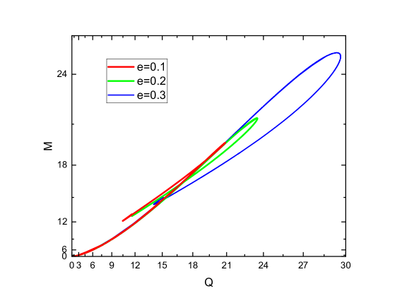
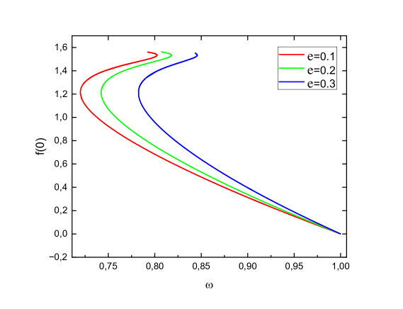
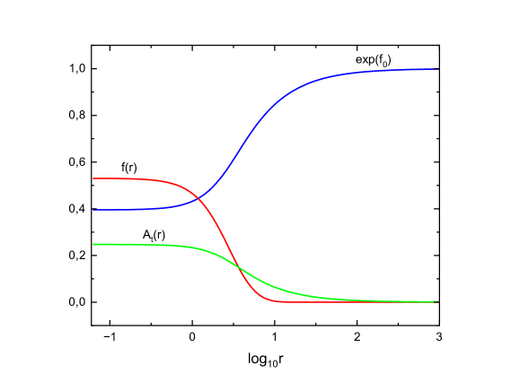
Figure 2: Spherically symmetric $U(1)$ gauged gravitating $O(3)$ solitons: The ADM mass (upper left) and the maximal value of the profile function $f(0)$ (bottom left) vs. frequency $\omega$ and the mass vs. Noether charge (upper right) are plotted for some set of values of the gauge coupling $e$ and for gravitational coupling $\alpha^{2}=1$. The profile functions of an illustrative solution on the first branch are plotted for gravitational coupling $\alpha^{2}=1$, frequency $\omega=0.85$, and gauge coupling $e=0.2$ (bottom right).

The basic properties of the $U(1)$ gauged gravitating $O(3)$ solutions so constructed can be summarized as follows:

The configurations possesses a core in which most energy is localized, and an asymptotic tail, which is responsible for the long-range interaction between the well-separated solitons. Similar to the usual boson stars, for a given value of the gauge coupling $e$ regular solutions exist for a limited range of frequencies $\omega\in[\omega_{min},1]$, where upper critical value corresponds to the mass threshold. The domain of existence of such $O(3)$ boson stars, in an ADM mass $M$ vs. angular frequency diagram is presented in Fig. 2, upper left plot.

The minimal critical frequency increases with $e$, our numerical results suggest that there is no branch of charged gravitating $O(3)$ solitons linked to the flat space limit in the model with the potential (3).

The frequency dependence of the solutions is qualitatively similar to that found for the charged boson stars, see Lee:1991ax ; Jetzer:1989av ; Jetzer:1989us ; Collodel:2019ohy ; Pugliese:2013gsa . As the angular frequency is decreased below the upper critical value $\omega_{max}=1$, a fundamental branch of charged self-gravitating solutions arises from the trivial scalar vacuum $\phi^{a}=(0,0,1)$. This branch extends backward up to a minimal value of the frequency $\omega_{min}$, at which it bifurcates with the second forward branch, see Fig. 2, upper left plot. Both the mass and the charge of the configuration reach the maximum values on the first branch at some critical frequency. The maximal value of the mass and the charge increases with $e$.

Subsequently, further bifurcations follow and a multi-branch structure arises providing an overall inspiralling pattern for the frequency dependency of both charge and mass of the fundamental $U(1)$ gauged gravitating $O(3)$ solitons. This behavior is typical for the usual boson stars, see Lee:1991ax ; Jetzer:1989av ; Jetzer:1989us . Both the mass and the charge of the configurations tend to some finite limiting values at the centers of the spirals. When following the spirals towards their centers, the maximal value of the field amplitude $f$ is increasing monotonically, as displayed in Fig. 2, bottom left plot. Similar to the case of the usual boson stars, the metric function $g_{00}$ at the center of the configuration approaches zero in this limit. However, the central value of the scalar amplitude cannot diverge because of the constraint of the non-linear $O(3)$ sigma model. We may conjecture that at the centers of the spirals this value approaches a finite limiting value $f(0)\sim\pi/2$, i.e. for a critical solution the $O(3)$ field becomes restricted to a circle $S^{1}$. In the spiral, the core of the configuration shrinks, however, the tail becomes more extended. At the same time, for the secondary branches of the spiral the numerical accuracy rapidly decreases, a different numerical approach is necessary for the study of this limit.

The contribution of the electromagnetic energy modifies the $M(Q)$ dependency Kleihaus:2007vf , see Fig. 2, upper right plot. The spikes of the uncharged case transforms into a set of loops, the size of the loops increases with $e$. More importantly, depending on the relative strength of gravity and the electromagnetic interaction, the gauged $O(3)$ boson stars exhibit different behavior in the limit $\omega\to 1$.

The gauged $O(3)$ configurations experience an additional repulsive interaction arising from the gauge sector, as gravitational coupling decreases, the relative contribution of the electrostatic energy becomes increasingly essential.

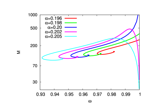
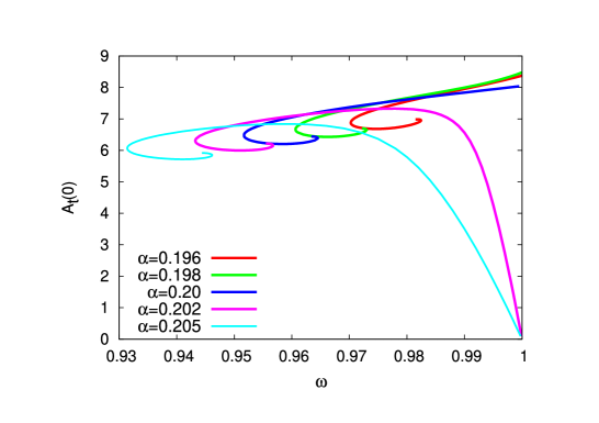
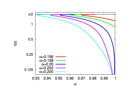
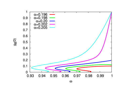
Figure 3: Spherically symmetric $U(1)$ gauged gravitating $O(3)$ solitons: The ADM mass (upper left plot) in units of $8\pi$, the value of the gauge potential $A_{0}$ at the origin (upper right plot), the value of the scalar profile function $f$ at the origin (bottom left plot) and the value of the metric function $g_{tt}$ at the origin vs. frequency $\omega$ (bottom right plot) are displayed for some set of values of the gravitational coupling $\alpha$ and for the gauge coupling $e=0.1$.

Given a value of the gravitational coupling $\alpha$, the minimal value of the angular frequency $\omega_{min}$ increases with $e$, see Fig. 2. For a given value of the frequency $\omega$, charged soliton solutions appear to exist up to a maximal value of the gauge coupling constant only. Physically, this pattern is related with the electrostatic repulsion which becomes stronger as $e$ increases.

For a fixed value of the gauge coupling $e$, decrease of the gravitational coupling $\alpha$ entails an increase of the minimal frequency $\omega_{min}$. Coincidentally, the secondary branches of the spiral become shorter. Importantly, the limiting behavior of the fundamental branch at $\omega\to 1$ depends on the relative strength of the gauge and gravitational couplings. However, the overall spiral pattern is always observed. For sufficiently large gauge coupling $e$ and sufficiently small gravitational coupling $\alpha$ the limit $\omega\to 1$ then is no longer Newtonian. This is illustrated in Fig. 3. It appears that, for a given value of the gauge coupling, there is a critical value of the gravitational constant $\alpha_{cr}$, at which the repulsive force of electrostatic interaction is balanced by the gravitational attraction. In particular, for $e=0.1$ the critical gravitational coupling is $\alpha_{cr}\approx 0.20$.

We notice that the usual Newtonian limit exists as $\alpha>\alpha_{cr}$. In this case, as $\omega\to 1$, the scalar field approaches the vacuum $\phi_{\infty}^{a}$, the metric attain flat space limit and the electrostatic potential is vanishing, see Fig. 3. The critical case corresponds to divergent ADM mass $M$ and the charge $Q$, both the metric function $N$ and the electric potential $A_{t}$ approach some finite non-zero values it the center of configuration, although the scalar field trivializes and decouples from the gauge sector.

A different scenario arises while $\alpha<\alpha_{cr}$, as demonstrated in Fig. 3. Then the fundamental branch is dominated by the electromagnetic interaction, the limit $\omega\to 1$ corresponds to the finite non-zero values of both the ADM mass $M$ and the charge $Q$, the scalar field is not in the vacuum, the electric potential remains finite and the spacetime is not flat. This pattern is qualitatively similar to that of the usual gauged boson stars Kunz:2021mbm .

III.3 Axially symmetric solutions (n=1)

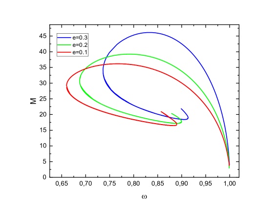
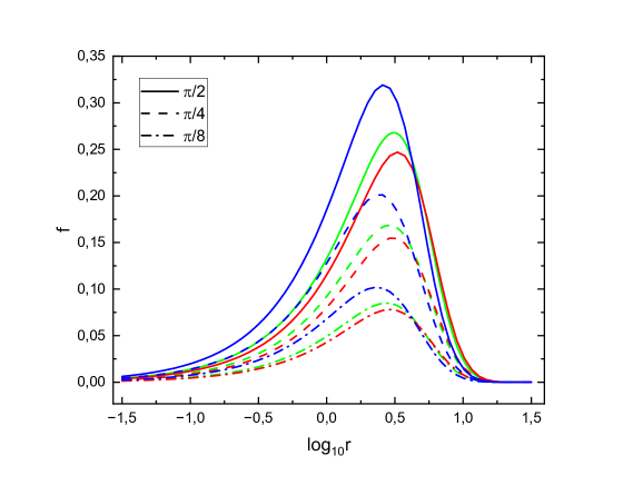
Figure 4: Axially symmetric $U(1)$ gauged gravitating $O(3)$ solitons: The ADM mass (left) vs. frequency $\omega$ and the scalar profile function $f$ of illustrative solutions on the first branch at $\omega=0.85$ (right) are plotted for some set of values of the gauge coupling $e$ and for the gravitational coupling $\alpha^{2}=1$.

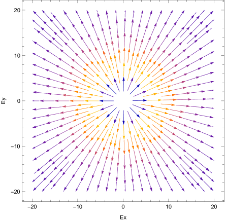
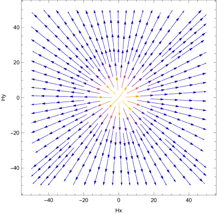
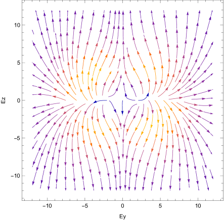
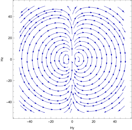
Figure 5: $U(1)$ gauged gravitating $O(3)$ solitons: Electromagnetic field orientation of an illustrative axially-symmetric (n=1) solution on the first branch is displayed for gravitational coupling $\alpha^{2}=1$, frequency $\omega=0.85$, and gauge coupling $e=0.2$: the electric (upper left) and magnetic (upper right) field fluxes in the x-y plane, and the electric (bottom left) and magnetic (bottom right) field fluxes in the y-z plane.

Spinning axially-symmetric $(n\geq 1)$ solitonic configurations are constructed as parity-even solutions of the system of equations (8), (10) with the stationary ansatz (13),(14) and (15), and the boundary conditions (20),(21),(22) and (23). We shall restrict our study to the case $n=1$, corresponding solutions are qualitatively similar to those of higher values of the azimuthal winding.

Apart from the sigma-model constraint, charged axially symmetric gravitating solutions of the $O(3)$ model are akin to the rotating $U(1)$ gauged boson stars Collodel:2019ohy . In both cases regular soliton solutions emerge similarly from the vacuum at the maximal frequency $\omega_{max}=1$. The scalar profile function $f$ has a pronounced maximum on the symmetry plane, as displayed in Fig. 4, right plot. The amplitude of the field becomes larger as the gauge coupling becomes stronger (with the other parameters fixed).

The dependency of these configurations on the angular frequency $\omega$ is qualitatively similar to that just described for the spherically symmetric solitons, the ADM mass of the spinning $n=1$ solutions increases as the frequency decreases below the threshold, it approaches its maximum at some value of the frequency $\omega<1$, see Fig. 4 left plot. The ADM mass and charge Q form a spiral, as $\omega$ is varied, while the metric function $f_{0}$ becomes exponentially small, see Fig. 6, bottom plot. The maximum of the scalar function $f$ on the equatorial plane shows damped oscillations towards a maximal value, the amplitude of the axially-symmetric field is always smaller than the corresponding value of the fundamental spherically-symmetric solutions, see Fig. 6, upper right plot.

The total angular momentum of the axially-symmetric solutions of the $O(3)$ sigma model can be evaluated from (17), as well as from the asymptotic decay of the metric function $W$. Recall that the charge $Q$ and the angular momentum are related via (19).

Axially symmetric configurations posses both electric and magnetic field, which is generated by the Noether current (4). The corresponding toroidal magnetic field encircles the soliton, as seen in Fig. 5. The electric charge of the configuration is vanishing at the center of the spinning gauged $n=1$ soliton, the nodal structure of the electric field is resembling the field of a circular charged loop, the radius of the loop corresponds to the characteristic size of the configuration, for a given value of the gauge coupling, it increases on the first fundamental branch of solutions until the maximal mass is attained; then the trend inverts and the size of the soliton decrease until the minimum ADM mass attained along the second branch. The solutions then follows a spiraling/oscillating pattern, with successive backbendings towards a limiting singular solution at the center of the spiral, which, however, possesses finite mass and charge. As before, the maximal value of the scalar field is restricted by the sigma-model constrain while it diverges for the usual boson stars.

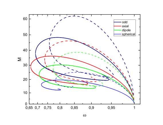
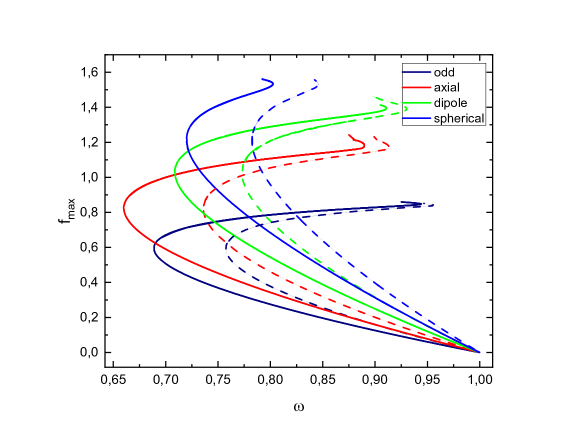
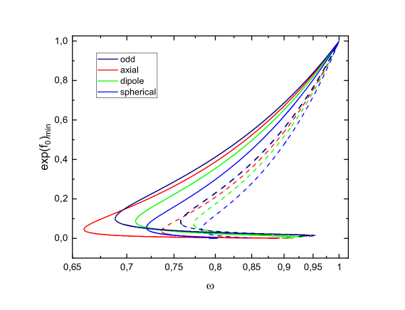
Figure 6: Different types of $U(1)$ gauged gravitating $O(3)$ solitons: The ADM mass (upper left), the maximal value of the scalar profile function $f$ (upper right) and the exponent of the metric function $f_{0}$ (bottom plot) are plotted vs. the frequency $\omega$ for two values of the gauge coupling $e=0.1$ (solid line) and $e=0.3$ (dashed line) and for gravitational coupling $\alpha^{2}=1$.

III.4 Parity-odd solutions (n=1)

By analogy with axially symmetric boson stars and spinning Q-balls in flat space Kleihaus:2005me ; Kleihaus:2007vk ; Radu:2008pp ; Kunz:2019bhm , for each non-zero value of the integer winding number $n$, there should be two types of spinning solutions of the non-linear $O(3)$ sigma-model possessing different parity, the parity-even and the parity-odd, respectively. Similar to the solutions of other types, the parity-odd configurations do not possess the flat space limit.

For the parity-odd solutions the scalar $O(3)$ field vanishes both on the z-axis and in the xy-plane, the energy density distribution exhibits a double torus-like structure, with two tori located symmetrically with respect to the equatorial plane, as illustrated in Fig. 1.

The dependence of these solutions on the frequency $\omega$ is qualitatively similar to that of the other spinning boson stars, as seen in Fig. 6. As expected, for the same set of values of the parameters of the model, the mass of the parity-odd configurations is higher than the mass of corresponding solutions of other types, see Fig. 6, upper left plot. The minimal frequency $\omega_{min}$ of the parity-odd configurations is higher than the analogous minimal frequency of the fundamental spherically-symmetric solution but smaller than the minimal frequency of the parity-even $n=1$ axially-symmetric configurations.

The mass of the parity-odd solution also exhibit a spiral structure towards a limiting solution. The spatial distribution of the $O(3)$ scalar field on the first branch exhibit two local extrema at $\theta=\pi/4,~3\pi/4$, see Fig. 7, left plot . As usual, the emergency of the frequency-mass spiral may be related to damped oscillations in the force-balance between the repulsive scalar interaction and the gravitational attraction in equilibrium. The electromagnetic interaction shifts the balance. In the spiral the gravitational attraction becomes stronger, the characteristic size of the localized configuration decreases. Interestingly, the shape of the distribution of the scalar field changes along the third branch of the spiral, it becomes more compact and a quadruple torus-like structure arises on the forth branch, see Fig. 7. This observation suggests that multi-torus configurations may arise on subsequent branches of the spiral.

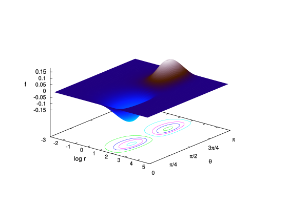
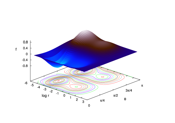
Figure 7: The $O(3)$ scalar field for $n=1$ negative parity solutions for the gauge coupling $e=0.1$ and gravitational coupling $\alpha^{2}=1$ at $\omega=0.86$ on the first (left) and the forth (right) branches versus the coordinates $\log r$ and $\theta$.

The maximal value of the scalar amplitude always remains smaller than for solutions of other types, approximately half the respective maximal value of the fundamental spherically-symmetric solution, see Fig. 6, upper right plot. Again, increase of the gauge coupling is related with a growing contribution of the electromagnetic forces, the secondary branches become less extended.

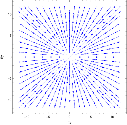
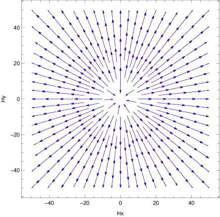
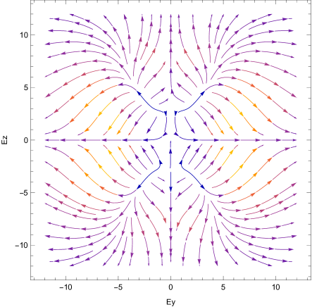
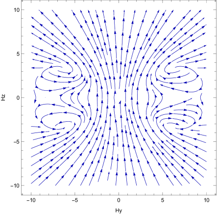
Figure 8: $U(1)$ gauged gravitating $O(3)$ solitons: Electromagnetic field orientation of an illustrative parity-odd (n=1) solution on the first branch is displayed for gravitational coupling $\alpha^{2}=1$, frequency $\omega=0.85$, and gauge coupling $e=0.2$: the electric (upper left) and magnetic (upper right) field fluxes in the x-y plane, and the electric (bottom left) and magnetic (bottom right) field fluxes in the y-z plane.

The $U(1)$ gauged parity-odd solutions posses both electric and magnetic field, which is generated by the Noether current (4). The configuration is encircled by a double toroidal flux, as displayed in Fig. 8, right plots. The corresponding electric field exhibit peculiar structure, see Fig. 8, left plots. It can be interpreted as being generated by two charged discs placed symmetrically with respect to the equatorial plane.

III.5 Dipole solutions (n=0)

We now turn to the dipole solution, which represents two non-spinning, $U(1)$ gauged $O(3)$ boson stars in equilibrium. These configurations resemble the corresponding two-center dipolar boson stars Yoshida:1997nd ; Herdeiro:2021mol ; Cunha:2022tvk ; Ildefonso:2023qty , they exist due to the balance between the gravitational attraction and the (short-range) scalar mediated repulsion. Long-range electrostatic interaction between the gauged $O(3)$ solitons shifts this balance, each component of the dipole possesses an electric charge, as shown in Fig. 11. For a given value of the gravitational coupling $\alpha$ an increase of the gauge coupling $g$ entails an increase of the electric charge and, subsequently, an increase of the equilibrium distance between the components.

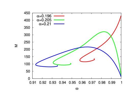
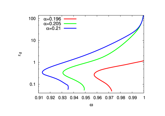
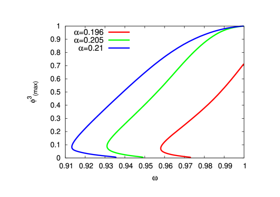
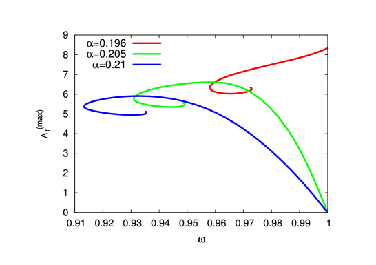
Figure 9: $U(1)$ gauged gravitating $O(3)$ dipole solitons: The ADM mass (upper left plot) in units of $8\pi$, the separation $z_{d}$ between the two components (upper right plot), the maximal value of the scalar component $\phi^{3}$ (bottom left plot) and the maximal value of the gauge potential $A_{0}$ (bottom right plot) vs. frequency $\omega$ are displayed for several values of the gravitational coupling $\alpha$ for the gauge coupling $e=0.1$.

The dipole solution can be considered as a limiting non-rotating ($n=0$) parity odd configuration of self-gravitating scalar field. Two components of the dipole are individual electrically charged boson stars with a phase difference of $\pi$ Herdeiro:2021mol ; Cunha:2022tvk . Indeed, inversion of the sign of the scalar field function under reflections $\theta\to\pi-\theta$ corresponds to the shift of the phase $\omega t\to\omega t-\pi$. Also, it was pointed out that the character of the interaction between Q-balls in Minkowski spacetime depends on their relative phase, it is attractive is the Q-balls are in phase, and it is repulsive if the Q-balls are in opposite phases Battye:2000qj .

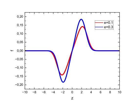
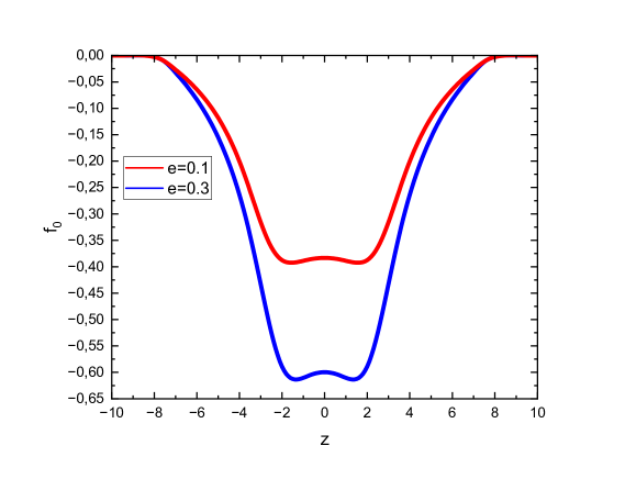
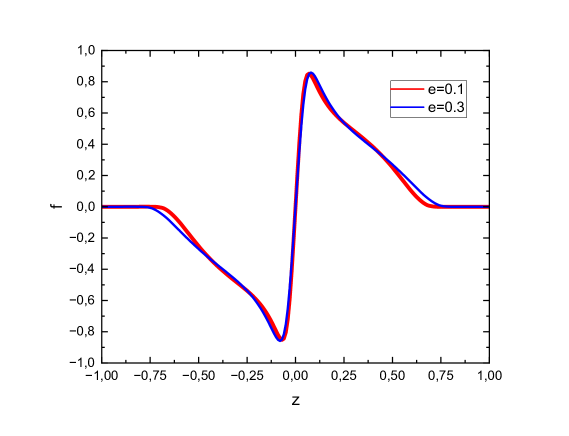
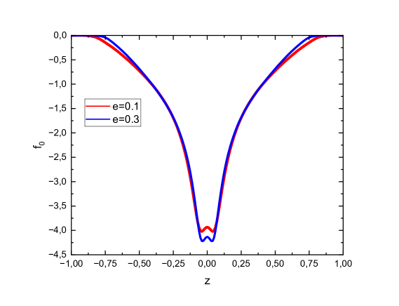
Figure 10: Profiles on the symmetry axis of the $O(3)$ scalar field function (left) and the metric function $f_{0}$ (right) of an illustrative $n=0$ dipole solutions on the first branch (upper plots) and on the third branch (lower plots) at $e=0.1$ and $e=0.3$ for gravitational coupling $\alpha^{2}=1$ and $\omega=0.885$. Here $z=r\cos\theta$ with $\theta=\frac{\pi}{4}$.

The dipole $O(3)$ configuration always possess two distinct components, located on the z-axis at $z=\pm z_{d}$, see Fig. 10.

As seen in Fig. 6, left plot, the mass-frequency dependence of the dipole $O(3)$ boson star looks qualitatively similar to that found for solutions of other types. When the electromagnetic interaction is weaker that the gravitational force, a fundamental branch of charged $O(3)$ dipoles emerge from the Newtonian limit, where both the mass and the charge vanish, the scalar field approaches the vacuum $\phi^{3}=1$ and the separation parameter $z_{d}$ becomes infinitely large, as demonstrated in Fig. 9. The gauged $O(3)$ dipole shows a spiraling behavior with an infinite number of branches toward a limiting configuration where the component of the scalar field $\phi^{3}$ approaches zero.

This pattern changes as the electrostatic repulsion becomes still stronger. The gauged $O(3)$ stars then show different behavior, the fundamental branch does not possess the Newtonian limit at the maximal frequency, see Fig. 9. Then, at the mass threshold, both the ADM mass and the Noether charge of the configuration are finite, as well as the separation between the components. The fundamental branch is followed by a spiral.

For a given frequency $\omega$ and the gauge coupling $e$, the mass of a dipole configuration is smaller than the mass of two spherically-symmetric gauged $O(3)$ boson stars with the same frequency. This is consistent with interpretation of the dipole as a bound state of two individual boson stars with negative binding energy.

We shall emphasize the important difference between the dipole of the boson stars in a theory of complex scalar field coupled to Einstein gravity Yoshida:1997nd ; Herdeiro:2021mol ; Cunha:2022tvk ; Ildefonso:2023qty and the corresponding self-gravitating solutions of the $O(3)$-non-linear sigma model. In the former case, the evolution along the spiral is related with an unrestricted growth of the magnitude of the scalar field while each component of the dipole becomes highly localized on the axis of symmetry. In contrast, the magnitude of the scalar field of the $O(3)$-non-linear sigma model cannot grow without limit, the spiral-like frequency dependence of the mass of the solutions towards a limiting solution is related with appearance of burls on the tail of the deformed configuration, see Fig. 10. The coordinate distance $d_{z}$ between the two separated components decreases and the position of two individual components of the dipole, associated the two antisymmetric peaks, is clearly related to the minima of the metric function $f_{0}$. Unfortunately, the approach toward the limiting solution is restricted by numerical accuracy of our scheme.

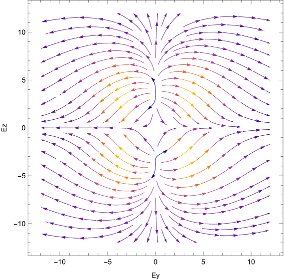
Figure 11: The electric field fluxes in the $y-z$ plane of an illustrative $n=0$ dipole solutions on the first branch for the gauge coupling $e=0.2$ and for gravitational coupling $\alpha^{2}=1$ and $\omega=0.85$.

Conclusions

In this paper we have discussed globally regular self-gravitating $U(1)$ gauged solutions of the $O(3)$ non-linear sigma-model with a symmetry breaking potential. Configurations of four different types are considered, (i) Fundamental spherically symmetric solutions, (ii) Axially symmetric spinning solutions with non-zero angular momentum, (iii) Parity-odd spinning solution with an angular node on the symmetry plane, and (iv) a gravitationally bound pair of solitons, the dipole. These configurations represent a few simple examples from an infinite tower of multipolar self-gravitating solutions of the $O(3)$ non-linear sigma-model, in particular, there are radially excited solutions which we do not consider here. All configurations are electrically charged with long-range Coulomb asymptotic of the electric field. The $U(1)$ gauged spinning solutions are also endowed with toroidal magnetic field with a magnetic dipole asymptotic of the gauge potential. These solitonic configurations do not have a regular flat spacetime limit, certain modification of the potential is necessary to support such solutions Verbin:2007fa ; Ferreira:2025xey .

Our results indicate a close resemblance with the case of the multi-component boson stars in the massive, complex Klein-Gordon field theory. In both situations regular self-gravitating solitonic solutions exist only in a limited frequency range, the charge and mass of solutions exhibit a spiral-like frequency dependence. In this context it is plausible that all multi-polar configurations of the boson stars reported in Herdeiro:2020kvf may also exist in the $O(3)$ non-linear sigma-model minimally coupled to Einstein gravity.

An essentially new feature of the $U(1)$ gauged gravitating $O(3)$ solutions is that the electromagnetic interaction may become stronger than gravitational attraction. Then the solutions do not possess the Newtonian limit.

Another feature of the gauged $O(3)$ boson stars is that the amplitude of the scalar field cannot increase without a limit, the spiraling pattern is related with deformation of the tail of the configurations.

An interesting extension of this work would be to study possible associated hairy black holes with an event horizon at the center of the configurations. Presence of the electromagnetic interaction allows to circumvent the no-hair theorem Mayo:1996mv and construct synchronized spherically-symmetric Reissner–Nordström black holes with charged $O(3)$ scalar hair by analogy with the solutions of the Einstein-Maxwell-scalar theory Herdeiro:2020xmb ; Hong:2020miv ; Kleihaus:2009kr . Further, it would be interesting to study $U(1)$ gauged dipole configurations endowed with a black hole at the center.

Another interesting question, which we hope to be addressing in the near future, is to investigate the morphology of the ergo-regions of rotating and electrically charged configurations, which may lead to a superradiant instability of boson stars Brito:2015oca ; Cardoso:2007az .

We note, finally, that all configurations reported in this work are topologically trivial. However, the $O(3)$ non-linear sigma-model in 3+1 dimensional asymptotically flat space also may support topologically non-trivial Hopfion solutions. An analogy with the $U(1)$ gauged self-gravitating Skyrmion Kirichenkov:2023omy ; Piette:1997ny ; Radu:2005jp suggests that the Einstein-Faddeev-Skyrme model may also support topologically trivial localized field configurations, aka pion stars Ioannidou:2006nn . Investigation of such solutions is an intriguing direction to explore.

References

- (1) J. A. Wheeler, Phys. Rev. 97 (1955), 511-536
- (2) P. Jetzer, Phys. Rept. 220 (1992), 163-227
- (3) F. E. Schunck and E. W. Mielke, Class. Quant. Grav. 20 (2003), R301-R356
- (4) S. L. Liebling and C. Palenzuela, Living Rev. Rel. 26 (2023) no.1, 1
- (5) Y. Shnir, Lect. Notes Phys. 1017 (2023), 347-362
- (6) D. J. Kaup, Phys. Rev. 172 (1968), 1331-1342
- (7) D. A. Feinblum and W. A. McKinley, Phys. Rev. 168 (1968) no.5, 1445
- (8) R. Ruffini and S. Bonazzola, Phys. Rev. 187 (1969), 1767-1783
- (9) M. Colpi, S. L. Shapiro and I. Wasserman, Phys. Rev. Lett. 57 (1986), 2485-2488
- (10) F. S. Guzman and J. M. Rueda-Becerril, Phys. Rev. D 80 (2009), 084023
- (11) D. F. Torres, S. Capozziello and G. Lambiase, Phys. Rev. D 62 (2000), 104012
- (12) H. Olivares, Z. Younsi, C. M. Fromm, M. De Laurentis, O. Porth, Y. Mizuno, H. Falcke, M. Kramer and L. Rezzolla, Mon. Not. Roy. Astron. Soc. 497 (2020) no.1, 521-535
- (13) E. W. Mielke and F. E. Schunck, Phys. Rev. D 66 (2002), 023503
- (14) F. E. Schunck, B. Fuchs and E. W. Mielke, Mon. Not. Roy. Astron. Soc. 369 (2006), 485-491
- (15) J. Chen, X. Du, E. W. Lentz, D. J. E. Marsh and J. C. Niemeyer, Phys. Rev. D 104 (2021) no.8, 083022
- (16) J. Preskill, M. B. Wise and F. Wilczek, Phys. Lett. B 120 (1983), 127-132
- (17) M. Dine and W. Fischler, Phys. Lett. B 120 (1983), 137-141
- (18) A. H. Guth, M. P. Hertzberg and C. Prescod-Weinstein, Phys. Rev. D 92 (2015) no.10, 103513
- (19) T. Matos and F. S. Guzman, Class. Quant. Grav. 17 (2000), L9-L16
- (20) A. Suárez, V. H. Robles and T. Matos, Astrophys. Space Sci. Proc. 38 (2014), 107-142
- (21) D. G. Levkov, A. G. Panin and I. I. Tkachev, Phys. Rev. Lett. 118 (2017) no.1, 011301
- (22) B. Kleihaus, J. Kunz and M. List, Phys. Rev. D 72 (2005) 064002 .
- (23) B. Kleihaus, J. Kunz, M. List and I. Schaffer, Phys. Rev. D 77 (2008) 064025
- (24) R. Friedberg, T. D. Lee and Y. Pang, Phys. Rev. D 35 (1987), 3658
- (25) G. Rosen, J. Math. Phys. 9 (1968), 996
- (26) R. Friedberg, T.D. Lee and A. Sirlin, Phys. Rev. D 13 (1976) 2739.
- (27) S.R. Coleman, Nucl. Phys. B 262 (1985) 263; Erratum: Nucl. Phys. B 269 (1986) 744
- (28) Y. Verbin, Phys. Rev. D 76 (2007), 085018
- (29) C. Herdeiro, I. Perapechka, E. Radu and Y. Shnir, JHEP 02 (2019), 111
- (30) C. Adam, J. C. Mourelle, A. García Martín-Caro and A. Wereszczynski, [arXiv:2502.20923 [gr-qc]].
- (31) P. A. Cano, L. Machet and C. Myin, Phys. Rev. D 109 (2024) no.4, 044043
- (32) S. Hod, Phys. Rev. D 86 (2012), 104026 [erratum: Phys. Rev. D 86 (2012), 129902]
- (33) C. A. R. Herdeiro and E. Radu, Phys. Rev. Lett. 112 (2014), 221101
- (34) G. H. Derrick, J. Math. Phys. 5 (1964), 1252-1254
- (35) D. A. Nicole, J. Phys. G 4 (1978), 1363 doi:10.1088/0305-4616/4/9/008
- (36) L. D. Faddeev, Lett. Math. Phys. 1 (1976), 289
- (37) Y. M. Shnir, J. Exp. Theor. Phys. 121 (2015) no.6, 991-997
- (38) C. A. R. Herdeiro, J. Kunz, I. Perapechka, E. Radu and Y. Shnir, Phys. Lett. B 812 (2021), 136027
- (39) S. Yoshida and Y. Eriguchi, Phys. Rev. D 55 (1997), 1994-2001
- (40) C. Herdeiro, I. Perapechka, E. Radu and Y. Shnir, Phys. Lett. B 797 (2019), 134845
- (41) P. Cunha, C. Herdeiro, E. Radu and Y. Shnir, Phys. Rev. D 106 (2022) no.12, 124039
- (42) C. Liang, C. A. R. Herdeiro and E. Radu, JHEP 03 (2025), 119
- (43) K. M. Lee, J. A. Stein-Schabes, R. Watkins and L. M. Widrow, Phys. Rev. D 39 (1989), 1665
- (44) K. N. Anagnostopoulos, M. Axenides, E. G. Floratos and N. Tetradis, Phys. Rev. D 64 (2001), 125006
- (45) I. E. Gulamov, E. Y. Nugaev and M. N. Smolyakov, Phys. Rev. D 89 (2014) no.8, 085006
- (46) I. E. Gulamov, E. Y. Nugaev, A. G. Panin and M. N. Smolyakov, Phys. Rev. D 92 (2015) no.4, 045011
- (47) J. Kunz, V. Loiko and Y. Shnir, Phys. Rev. D 105 (2022) no.8, 085013
- (48) P. Ildefonso, M. Zilhão, C. Herdeiro, E. Radu and N. M. Santos, Phys. Rev. D 108 (2023) no.6, 064011
- (49) R. Battye and P. Sutcliffe, Nucl. Phys. B 590 (2000), 329-363
- (50) R. S. Ward, J. Math. Phys. 44 (2003), 3555-3561
- (51) D. Harland, J. Jäykkä, Y. Shnir and M. Speight, J. Phys. A 46 (2013), 225402
- (52) R. A. Battye and M. Haberichter, Phys. Rev. D 87 (2013) no.10, 105003
- (53) R. Brito, V. Cardoso and P. Pani, Physics,” Lect. Notes Phys. 906 (2015), pp.1-237 2020,
- (54) C. A. R. Herdeiro and E. Radu, Eur. Phys. J. C 80 (2020) no.5, 390
- (55) J. P. Hong, M. Suzuki and M. Yamada, Phys. Rev. Lett. 125 (2020) no.11, 111104
- (56) J. P. Hong, M. Suzuki and M. Yamada, Phys. Lett. B 803 (2020), 135324
- (57) B. J. Schroers, Phys. Lett. B 356 (1995), 291-296
- (58) Y. Amari, M. Eto and M. Nitta, JHEP 11 (2024), 127
- (59) A. Y. Loginov, Phys. Rev. D 93 (2016) no.6, 065009
- (60) P. K. Ghosh and S. K. Ghosh, Phys. Lett. B 366 (1996), 199-204
- (61) A. Samoilenka and Y. Shnir, Phys. Rev. D 93 (2016) no.6, 065018
- (62) R. A. Leese, M. Peyrard and W. J. Zakrzewski, Nonlinearity 3 (1990), 773-808
- (63) P. Salmi and P. Sutcliffe, J. Phys. A 48 (2015) no.3, 035401
- (64) M. Gillard, D. Harland and M. Speight, Nucl. Phys. B 895 (2015), 272-287
- (65) T. D. Lee and Y. Pang, Phys. Rept. 221 (1992), 251-350
- (66) S. Carloni and J. L. Rosa, Phys. Rev. D 100 (2019) no.2, 025014
- (67) R. A. Battye, M. Haberichter and S. Krusch, Phys. Rev. D 90 (2014) no.12, 125035
- (68) T. Ioannidou, B. Kleihaus and J. Kunz, Phys. Lett. B 643 (2006), 213-220
- (69) I. Perapechka and Y. Shnir, Phys. Rev. D 96 (2017) no.12, 125006
- (70) C. Herdeiro, I. Perapechka, E. Radu and Y. Shnir, JHEP 10 (2018), 119
- (71) R. Kirichenkov, J. Kunz, N. Sawado and Y. Shnir, Phys. Rev. D 109 (2024) no.4, 045002
- (72) L. R. Livramento, E. Radu and Y. Shnir, SIGMA 19 (2023), 042
- (73) L. R. Livramento and Y. Shnir, Phys. Rev. D 108 (2023) no.6, 065010
- (74) F. E. Schunck and E. W. Mielke, Phys. Lett. A 249 (1998), 389-394
- (75) L.G. Collodel, B. Kleihaus and J. Kunz, Phys. Rev. D 99 (2019) no.10, 104076
- (76) C. Herdeiro, I. Perapechka, E. Radu and Y. Shnir, Phys. Lett. B 824 (2022), 136811
- (77) C. A. R. Herdeiro, J. Kunz, I. Perapechka, E. Radu and Y. Shnir, Phys. Rev. D 103 (2021) no.6, 065009
- (78) S. Stotyn, M. Chanona and R. B. Mann, Phys. Rev. D 89 (2014) no.4, 044018
-
(79)
N. I. M. Gould, J. A. Scout and Y. Hu,
ACM Transactions on Mathematical Software
33 (2007) 10; - (80) J. Kunz, I. Perapechka, and Y. Shnir, JHEP 07, 109 (2019).
- (81) P. Jetzer and J. J. van der Bij, Phys. Lett. B 227 (1989), 341-346
- (82) P. Jetzer, Phys. Lett. B 231 (1989), 433-438
- (83) D. Pugliese, H. Quevedo, J. A. Rueda H. and R. Ruffini, Phys. Rev. D 88 (2013), 024053
- (84) B. Kleihaus, J. Kunz, F. Navarro-Lerida and U. Neemann, Gen. Rel. Grav. 40 (2008), 1279-1310
- (85) E. Radu and M. S. Volkov, Phys. Rept. 468 (2008), 101-151
- (86) J. Kunz, I. Perapechka and Y. Shnir, Phys. Rev. D 100 (2019) no.6, 064032
- (87) L. A. Ferreira, A. Mikhaliuk and Y. Shnir, [arXiv:2503.06315 [hep-th]].
- (88) A. E. Mayo and J. D. Bekenstein, Phys. Rev. D 54 (1996), 5059-5069
- (89) B. Kleihaus, J. Kunz, C. Lammerzahl and M. List, Phys. Lett. B 675 (2009), 102-115
- (90) V. Cardoso, P. Pani, M. Cadoni and M. Cavaglia, Phys. Rev. D 77 (2008), 124044
- (91) B. M. A. G. Piette and D. H. Tchrakian, Phys. Rev. D 62 (2000), 025020
- (92) E. Radu and D. H. Tchrakian, Phys. Lett. B 632 (2006), 109-113