Realization of tunable spectral shift and linewidth reduction of Fano resonances at a dielectric metasurface due to near-field interactions among multipole moments

Abstract

Fano resonance is a well-known phenomenon in fields like atomic physics and grating optics, and it has recently started to gain interest in artificially engineered dielectric, metallic or composite metasurfaces, and metamaterials, to name a few. This work elucidates the role of the induced multipole moments within a dielectric metasurface that leads to the interference, and the resulting scattering response in the far-field emerges into Fano resonance. Here, we report the details of the interference between fields generated by induced multipole moments and their effect on the scattered response when a maneuvered change in the excitation source is applied from the far-field plane wave excitation to a dipole emitter interacting in the near-field of the metasurface. This change in excitation leads to observed effects like resonance red-shift and linewidth narrowing for the out-coupled scattering. Starting from Maxwell’s equations, we follow Feshbach formalism for electromagnetic scattering applied to the all-dielectric nanostructure used in this work, which leads us to satisfactory qualitative explanations along with the relevant results obtained from numerical calculations to support the observations we made experimentally. This work could help to explain and explore possibilities to observe asymmetric resonances in metasurfaces for various excitation conditions, and the key results of resonance shift and linewidth narrowing could be significant for precision applications and fundamental optical studies.

I INTRODUCTION

U. Fano explained the famous auto-ionization of atoms and the corresponding asymmetric line shape of the resonance, now commonly known as the Fano interference or Fano resonance. [1]. The description of the resonance did not remain limited to atomic physics but later became important and much studied in the research fields of gratings as Wood’s anomalies [2, 3, 4, 5], photonic crystals and metamaterials made of dielectric and metal-dielectric composites [6, 7, 8], etc. Recently, it is also observed in plasmonic nanostructures [9, 10, 11, 12, 13] and 2D plasmonic crystals [14, 15], the plasmonic analogue of electromagnetically induced transparency (EIT) in metamaterials [16, 17, 18], etc.
Fano resonances are usually sharp in the spectrum, and their asymmetric nature exhibits a strong sensitivity to the local environment changes where the interference occurs. Fano resonance is a general wave phenomenon. It is observed in nanoscale structures [12, 19, 20, 21, 22, 23] and finds applications in sensing with much higher precision [24], optical modulation, switching, etc. [25] which is well-appreciated nowadays. Optical resonances supported by subwavelength nanostructures swept across a broader range of interests for applications and fundamental studies [26, 27, 28, 29, 30, 31]. The reason behind the interference occurring in the subwavelength meta-structure systems remained obscure and needs a detailed experimental and theoretical investigation. This asymmetric resonance stems from the interference between a discrete non-radiative (dark) mode and the radiative (bright) mode continuum. The challenge is identifying those modes and their interference to understand the phenomenon at a fundamental level.
Optical resonances in the engineered nanostructures are supported by the induced dipole or multipole moments, like the electric dipole, magnetic dipole, and toroidal dipole [32, 33, 34, 35, 36]. Toroidal dipole moment is generated by the induced current loops along the surface of a torus through its meridians. This dipole moment was introduced in the nuclear and particle physics [37] but remained disregarded in natural media due to its weak response. Toroidal dipole moments have been studied for sensing and optical modulations in plasmonic or graphene-dielectric metasurface systems [38, 39, 40], but were not counted for all-dielectric metasurfaces in the visible or near-infrared region of the spectrum until recent times [41, 42, 43]. C. Zhou et al. experimentally demonstrated that toroidal dipole moments contribute to asymmetric resonances of the near-infrared spectrum of silicon-made nanohole metasurface [44] and quantified that by applying the multipole decomposition at the near-field. This work shows that the high refractive-index dielectric metasurfaces support induced multipole moments in a significant amount, which makes the system favorable for the emergence of Fano resonances.

In this work, we aim to understand the origin of specific observations we made in our recent experiments. We have observed the emergence of the asymmetric Fano-like resonance lineshape in a dielectric guided mode resonance metasurface (GMR-MSR, or simply MSR) and found that asymmetric resonance is robust for the MSR to couple with quantum emitters. This coupling allows the system to show intriguing observations like resonance redshift or further resonance linewidth narrowing, etc., compared to results obtained for the planewave excitation [45]. Here, we have theoretically investigated their origin and explained the observations with the help of numerical calculations. We started with the emergence of Fano resonance in this MSR. We numerically explained the origin of resonance redshift, linewidth narrowing, etc., comparing the results calculated for both sources, i.e., the planewave and the dipole. Numerical calculations followed the ab initio theory of the Fano resonance for electromagnetic scattering from a dielectric or metallic object in a dielectric background, based on the Feshbach formalism [46, 47, 48, 49]. Gallinet and Martin have developed this ab initio theory for plasmonic nanostructures [50]. Our numerical results confirm the applicability of the theory in a dielectric GMR-MSR system and explain the experimental observations. Numerical simulations were performed using the finite difference time domain (FDTD) method (©FDTD: 3D Electromagnetic Simulator, Lumerical Inc. [51]).
In the next sections, we will briefly discuss the theory used in our works and then present our numerical results to explain the observed Fano resonance from the decomposition of the fields due to induced multipole moments; then, we will present the key results of the far-field spectrum, e.g., the linewidth narrowing and resonance redshift. In the end, we will discuss in detail a glitch only found in the numerically calculated far-field spectrum, which could create confusion and raise questions about the theory’s applicability. We have explained its reason, which is inherited in the simulation setup.

II Theoretical methods

II.1 Brief introduction to the Electromagnetic theory of Fano resonances

We would start with Maxwell’s equation in a dispersing medium where the dielectric scatterer is present as the nanostructure. The dielectric nanohole array GMR-MSR simulated in this work is similar to what has been introduced by D. Rout, et al. [52] and used in [45] for numerical calculations. Detailed derivations of theoretical methods used in this work are presented in Appendix A. The wave equation [Eq.(19)] is presented here in terms of the vector wave function of the electric field, $\ket{\textbf{E}}$. The field is assumed to follow harmonic time dependence $\textbf{E}=\textbf{E}_{0}e^{-i\omega t}$ throughout the paper.

Feshbach formalism as presented in [50, 46, 47, 48, 49] introduces the orthogonal projection operators $P$ and $Q$, which split the field wave function into radiative (bright) and non-radiative (dark) parts, and $P\ket{\textbf{E}}$ satisfies the radiation condition in the far field. Therefore, $Q$ has the orthonormal eigenfunction $\ket{\textbf{E}_{d}}$, the unique non-radiative mode with eigenvalue $z_{d}^{2}$ [Eq.(29)]. Here, $z_{d}=\omega_{d}+i\gamma_{d}$, $\omega_{d}$ is the resonance frequency, and $\gamma_{d}$ is the resonance width due to intrinsic damping. The system should be studied near the resonance frequency $\omega_{d}$ to enact the operator $Q$. Around the resonance frequency, it can be shown that $Q$ is expanded w.r.t its eigenfunctions $\ket{\textbf{E}_{d}}$ only [Eq.(30)] [48]. Introducing $P$ and $Q$ in Eq.(21) leads to two coupled equations of operators $P$ and $Q$ [Eq.(27)-Eq.(28)]. Those two coupled equations modify Eq.(21) with a frequency-dependent source term,

$$(\mathcal{M^{\prime}}_{\omega}-\omega^{2}\textbf{I})P\ket{\textbf{E}}=-P\mathcal{M}_{\omega}\ket{\textbf{E}_{d}}\left[\frac{1}{(\omega^{2}-z_{d}^{2})}\right]\bra{\textbf{E}_{d}}\mathcal{M}_{\omega}P\ket{\textbf{E}},$$ (1)

$\mathcal{M^{\prime}}_{\omega}$, which is modified from the differential operator $\mathcal{M}_{\omega}$ of the wave equation [Eq.(20)], is defined in Eq.(35-36).
The bright part of the wavefunction $\ket{P\textbf{E}_{b}}$ satisfies the homogeneous solution of Eq.(1),

$$(\mathcal{M^{\prime}}_{\omega}-\omega^{2}\textbf{I})\ket{P\textbf{E}_{b}}=0$$ (2)

The dyadic Green’s function $\mathcal{G}_{b}$ of Eq.(2) is used to solve Eq.(1). The solution comes out as,

$$P\ket{\tilde{\textbf{E}}}=\ket{P\textbf{E}_{b}}+\frac{\bra{\textbf{E}_{d}}\mathcal{M}_{\omega}\ket{P\textbf{E}_{b}}}{z_{d}^{2}-\omega^{2}+\omega_{d}\Delta}\mathcal{G}_{b}P\mathcal{M}_{\omega}Q\ket{\textbf{E}_{d}},$$ (3)

$$\text{where,}\;\;\Delta=-\frac{\bra{\textbf{E}_{d}}\mathcal{M}_{\omega}P\mathcal{G}_{b}P\mathcal{M}_{\omega}\ket{\textbf{E}_{d}}}{\omega_{d}}$$ (4)

Here, $\Delta$ is the resonance shift in the frequency for the scattering after the interference occurs between bright and dark mode wavefunctions. Note the negative sign in Eq.(4). This signifies the frequency redshift of the scattering resonance. The wavefunction $\ket{\tilde{\textbf{E}}}$ is related to $\ket{\textbf{E}}$ but does not carry the same asymptotic behavior.
Defining the dyadic Green’s function $\mathcal{G}_{b}$ in terms of the wavefunction of the field continuum [Eq.(43)], Eq.(3) can be simplified to

$$P\ket{\tilde{\textbf{E}}}=\ket{P\textbf{E}_{b}}\left[1+\frac{\left|\bra{\textbf{E}_{d}}\mathcal{M}_{\omega}\ket{P\textbf{E}_{b}}\right|^{2}}{2\omega(z_{d}^{2}-\omega^{2}-\omega_{d}\Delta)}i\right]$$ (5)

Whereto, the intrinsic damping parameter and resonance width can be defined, brought out of the interference between the field continuum with the discrete part.

$$\Gamma_{i}=\frac{\left|\bra{\textbf{E}_{d}}\mathcal{M}_{\omega}\ket{P\textbf{E}_{b}}\right|^{2}\gamma_{d}\omega_{d}}{\omega(z_{d}^{2}-\omega^{2}+\omega_{d}\Delta)^{2}},$$ (6)

$$\Gamma=\frac{\left|\bra{\textbf{E}_{d}}\mathcal{M}_{\omega}\ket{P\textbf{E}_{b}}\right|^{2}}{2\omega(1-\Gamma_{i})},$$ (7)

The field term $\ket{\tilde{\textbf{E}}}$ is introduced to connect $\ket{\textbf{E}}$ with $\ket{\textbf{E}_{b}}$ in the far field to obtain the same normalization between them (i.e., $\left|P\ket{\textbf{E}}\right|^{2}=\left|\ket{P\textbf{E}_{b}}\right|^{2}$). Therefore, the required relation between $\ket{\textbf{E}}$ and $\ket{\tilde{\textbf{E}}}$ is,

$$\ket{\textbf{E}}=\frac{\cos{\eta\ket{\tilde{\textbf{E}}}}}{(1-\Gamma_{i})}$$ (8)

Here $\cot{\eta}=\kappa$, and $\kappa$ is defined as the reduced frequency after the interference,

$$\kappa=\frac{\omega^{2}-\omega_{d}^{2}-\omega_{d}\Delta}{\Gamma}$$ (9)

Starting from Eq.(3) to Eq.(9), all results are the emergence of field overlap between the continuum of the bright field $\ket{P\textbf{E}_{b}}$ and the discrete dark mode $\ket{\textbf{E}_{d}}$; the extent of that overlap defines the strength of interference. That strength tunes the observed effects in the far-field spectrum.
Significance of $\eta$ appears in the asymptotic relation between the total field wavefunction $\ket{\textbf{E}}$ and bright field continuum $\ket{\textbf{E}_{b}}$;

$$P\ket{\textbf{E}}=P\ket{\textbf{E}_{b}}\exp{i\eta}$$ (10)

This term rapidly shifts the phase of $\ket{\textbf{E}}$ by $\sim\pi$ in the frequency region $\Gamma$ around the resonance. Since $\eta$ is a complex number, it affects the resonance linewidth of the frequency spectrum in the far field.
The resonance redshift, intrinsic damping, resonance width, and Eq.(10) are the key expressions for this work. Our prime results are the comparative study of the numerical results of these expressions obtained for an unpolarized broadband planewave source and a dipole source. The dipole source is embedded in the MSR, sitting at the bottom of the etches of the nanohole array. This scheme was applied in our previous work [45] for the maximal near-field coupling of the dipole radiation field and the MSR mode. Since the MSR is square-symmetric along its plane, we only need to consider two different polarizations of the dipole source throughout calculations, the vertical and the horizontal polarization w.r.t the MSR plane.

II.2 Multipole Decomposition of Induced Moments in the Metasurface to Realize the Fano Resonance

Numerical calculations need the decomposition of the MSR scattering response from the induced multipoles in a unit cell. The multipole moment decomposition of the scattering response for Cartesian coordinates has been defined following these articles [44, 53]; the induced current density j in a unit cell of the circular nanohole MSR is given by

$$\textbf{j}=-i\omega\epsilon_{0}(n^{2}-1)\textbf{E}$$ (11)

where E is the local scattering electric field at the MSR unit cell, and $n$ is the refractive index of the MSR material. From this current density j, induced multipole moments can be defined;

$$\textbf{P}=\frac{1}{i\omega}\int\textbf{j}d^{3}r,$$ (12)

$$\textbf{M}=\frac{1}{2c}\int(\textbf{r}\times\textbf{j})d^{3}r,$$ (13)

$$\textbf{T}=\frac{1}{10c}\int[(\textbf{r}\cdot\textbf{j})\textbf{r}-2r^{2}\textbf{j}]d^{3}r,$$ (14)

$c$ and $\omega$ represent the incident light’s speed and angular frequency, respectively. P, M, and T define the induced electric dipole moment (ED), magnetic dipole moment (MD) and toroidal dipole moment (TD), respectively. Local scattering intensities of these individual moments can also be calculated;

$$I_{P}=\frac{2\omega^{4}}{3c^{3}}\left|\textbf{P}\right|^{2},$$ (15)

$$I_{M}=\frac{2\omega^{4}}{3c^{3}}\left|\textbf{M}\right|^{2},$$ (16)

$$I_{T}=\frac{2\omega^{6}}{3c^{5}}\left|\textbf{T}\right|^{2}$$ (17)

Following the decomposition [Eq.(12-14)], modes for bright and dark parts of the wavefunction can be separated, as those are used to define the expressions in section II.1.

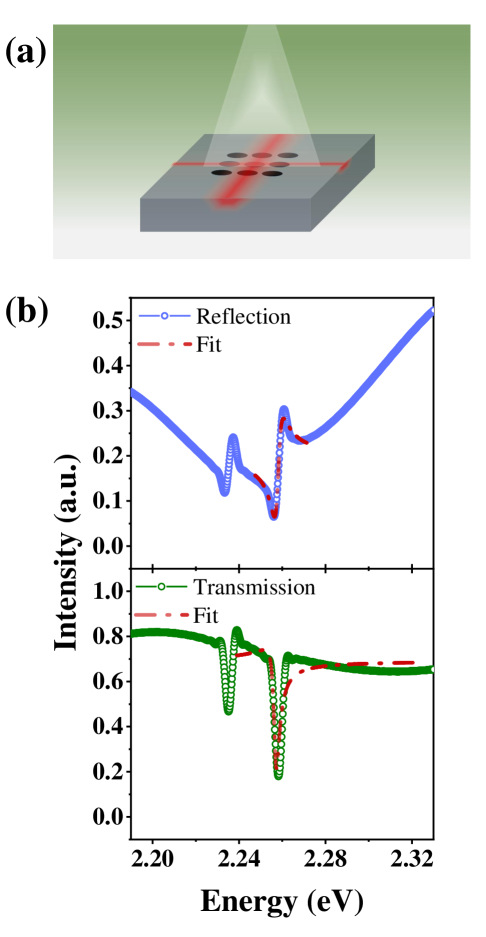
Figure 1: (a) Schematic of nanohole array metasurface excited with an incident plane wave field that generates the asymmetric resonance in the scattering, also gets guided through the underlined waveguide structure as depicted. (b) Simulated far-field spectra of the normalized scattering and transmission of the MSR under planewave excitation.

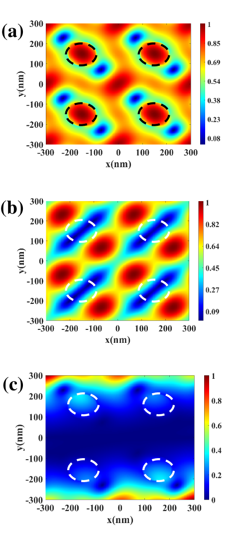
Figure 2: Numerical field profiles of multipoles defined in Eq.(12-14), obtained from the scattering response inside nanoholes. (a) shows field profile for P, (b) shows for M, and (c) shows for T, respectively, at the resonance frequency. Marked circles describe the positions of MSR etch-nanoholes.

III Results

Figure 1.(a) shows the graphical schematic of the dielectric GMR-MSR. An array of nanoholes is etched over the slab waveguide, which transports the guided mode. Numerical simulations were performed using the FDTD method with commercially available package software [51] to obtain the relevant results from the MSR system. The simulated MSR is a square lattice of circular nanohole array patterned into the Silicon Nitride (SiN) slab waveguide. Simulations are performed keeping the nanohole diameter at 120 nm and the periodicity at 300 nm for the unit cell. We have used the value of $n=1.933$ for SiN in this work. Following our previous works, these parameters have been maintained [45, 52]. The experimental system has MSR dimensions $\sim 1$ mm, accommodating $\sim 10^{6}$ nanoholes in the device. Our numerical results concern the far-field scattering spectra in frequency space; therefore, simulations were performed with one unit cell and periodic boundary conditions along the MSR plane. Simulated scattering responses of the MSR have been recorded by a field monitor placed at the MSR plane inside the nanohole. Corresponding normalized far-field scattering and transmission spectra are shown in Fig.1.(b). For presentation purposes, the schematic and field profiles are shown in symmetric arrangements. Figure 2 shows the scattering fields decomposed into individual contributions as defined by Eq.(12-14) at the MSR plane within nanoholes. All the field data were recorded with a field monitor placed along the MSR plane inside the nanohole of the unit cell. Further details of the simulations are mentioned in supplemental materials [54].

III.1 MSR excitation with the planewave source

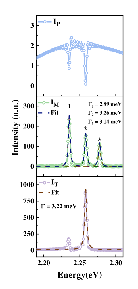
Figure 3: Numerical local scattering intensity plots for respective induced moments of ED, MD, and TD in MSR as expressed in Eq.(15-17), under planewave excitation.

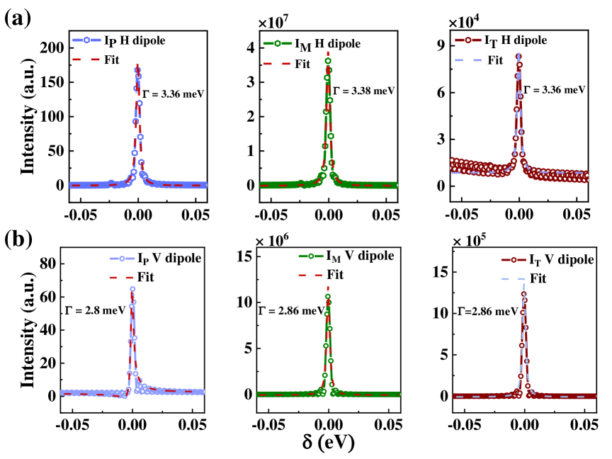
Figure 4: Plots are shown for the local scattering responses from the induced moments after exciting the MSR with the embedded dipole source. Here, $\delta\equiv\omega-\omega_{d}$. Results for the electric dipole, magnetic dipole, and toroidal dipole moments are mentioned as I_P, I_M, and I_T, respectively. The dipole is polarized parallel (H) and corresponding results are shown in panel (a), and perpendicular (V), results are shown in panel (b), to the plane of the MSR.

In the beginning, we used a planewave excitation in the simulation. Figure 3 shows the numerical local scattering intensity plots for respective induced moments inside the nanohole at the MSR plane, defined by Eq.(15-17). This plot provides two significant results. First, the induced electric dipole yields a field continuum in the frequency space, whereas contributions from other moments are discrete. Second, the induced toroidal dipole moment provides the maximum local scattering. Therefore, the field generated by ED is acting as the bright field continuum, and fields coming out of MD and TD with discrete modes interfere with the continuum, which entails the Fano resonance in the MSR at far-field, as shown in Fig.1(b). The resonance linewidth is $\sim 4.1$ meV.

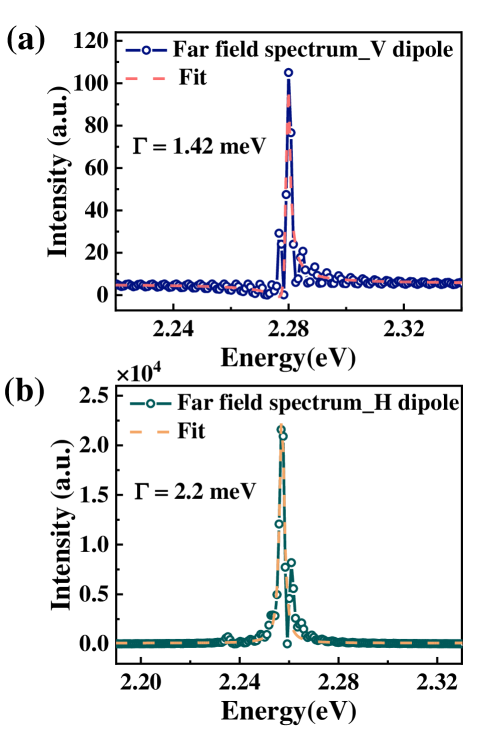
Figure 5: (a)&(b) Far-field spectrum for the dipole coupled scattering from the MSR for horizontal (H dipole) and vertical (V dipole) polarizations.

III.2 MSR excitation with the dipole source

In the next simulation, a dipole source was embedded in the MSR nanohole, and that excited the MSR at the near-field. The MSR array is square symmetric along its plane, therefore, dipole polarized perpendicular (denoted as vertical or V) and parallel (denoted as horizontal or H) to the MSR plane were used during the simulation. A significant enhancement is observed for respective local scattering intensities corresponding to Eq.(15-17). Those are shown in Fig.4.(a) and (b), for H and V dipole excitations, respectively. It should be noted that scattering responses by ED excited by the H dipole is a discrete mode at the resonance, but for the V dipole, this scattering response is a continuum (i.e., it is nonzero) in the given frequency range of interest.

III.3 Comparison of scattering results between two sources

Numerical results of local scattering responses $\ket{\textbf{PE}_{b}}$ and $\ket{\textbf{E}_{d}}$ are now obtained for both the excitations, defined by Eq.(12-14). Hence, $\Delta$ from Eq.(4) can be calculated and compared for the change of the excitation at the resonance frequency $\omega_{d}$. The data for resonance redshift $\Delta$ is given in Table 1 for the planewave excitation and the embedded dipole excitation of the MSR.

Table 1: Data for the frequency redshift $\Delta$ of the MSR scattering response for MSR excitations with planewave and dipole sources at $\omega_{d}$.

Excitation	Interference	Resonance redshift
source	between	$\Delta$ (Hz)
Planewave	ED-MD	29.807
	ED-TD	11.087
V dipole	ED-MD	8.265
	ED-TD	700.411
H dipole	ED-MD	$3.224\times 10^{4}$
	ED-TD	$2.257\times 10^{3}$

An increased magnitude of $\Delta$ obtained for the dipole excitation compared to the planewave would entail the observed resonance redshift. The shift and its amount are defined by Eq.(3-4). $\omega_{d}\Delta$ has a unit Hz². Thus, the shift amount is $\sqrt{\omega_{d}\Delta}$. Here, for the resonance frequency $\sim 2.254$ eV ($\approx 5.45\times 10^{14}$ Hz), total $\sqrt{\omega_{d}\Delta}$ amounts $\approx 1\,\mu$eV for the V dipole, and $\approx 7.15\,\mu$eV for the H dipole, respectively. These values are obtained by a single dipole interacting with one unit cell of the MSR at infinite periodic boundaries. From Eq.(4) and Eq.(43), it is evident that the stronger the field overlaps between $\ket{\textbf{PE}_{b}}$ and $\ket{\textbf{E}_{d}}$, the stronger the interference would be, eventually increasing the magnitude of the frequency shift.

$\Gamma_{i}$ and $\Gamma$ defined in Eq.(6-7) also increase due to the increase in the interference. This is caused due to enhanced scattering by induced moments for the embedded dipole excitation of the MSR. However, the far-field response after the interference shows the resonance linewidth narrowing compared to planewave excitation. Figure 5.(a) & (b) show the far-field scattering response of the MSR for the embedded dipole source of both polarizations, defined by Eq.(10). Resonance linewidth reduces $\sim 65\%$ for the V dipole and $\sim 46\%$ for the H dipole. The phase term in Eq.(10) is responsible for further narrowing once the excitation is changed from the planewave to the dipole source. Since $z_{d}$ is a complex quantity [Eq.(29)], hence the complex input remains in Eq.(4) and Eq.(9-10), that yield $\eta$ as a complex number. Therefore, from Eq.(10), the imaginary part of $\eta$ will remain in $\left|P\ket{\textbf{E}}\right|^{2}$ as $\exp(-2\Im{\eta})$; that squeezes the mode in the frequency range of $\Gamma$ around the resonance. Hence, an increase in $2\imaginary(\eta)$ would narrow the resonance linewidth in the far field.

Table 2: Summary of the Fano asymmetry factor ($q$), far-field resonance linewidth $\Gamma_{ff}$, the reduction of $\Gamma_{ff}$, total 2Im$(\eta)$, total $\Gamma$, their difference and the reduction factor. Here, N.A. means that it does not apply to the respective term.

Excitation	$q$	$\Gamma_{ff}$	Reduction	2Im($\eta$)	$\Gamma$	Reduction
source		(meV)	(for $\Gamma_{ff})$		(a.u,)	(between $\Gamma$ and $\eta$)
Planewave	0.905	4.1	N.A.	81.8	41.1	N.A.
V dipole	2.593	1.42	0.654	1471.4	532.54	0.653
H dipole	N.A.	2.20	0.463	69020	34578.1	0.499

The trade-off between the increment in the resonance width $\Gamma$ and the increment in the magnitude of $2\imaginary(\eta)$ is observed in the far-field spectra (Fig.5). From the definition of Eq.(8-9), it is evident that $\eta$ and $\Gamma$ are connected, and all these terms stem from the interference. Since the far-field linewidth has the term 2Im($\eta$), i.e., twice the parameter of Im($\eta$), that is always greater and would reduce the overall linewidth when there is an increased overlap between the bright mode continuum and the dark mode, i.e., a stronger interference. This has been explained with a detailed break-up of values for relevant parameters in Table I in the supplemental materials [54].
Table 2 shows the comprehensive summary of parameters relevant in far-field spectra. Here, the asymmetry factor $q$ for the Fano resonance (defined in Eq.(51) in Appendix A), resonance linewidth, the reduction of linewidth due to dipole excitation, 2Im$(\eta)$ and $\Gamma$ for each excitation, and their corresponding overall reductions are discussed. This table presents the prime results of the observed Fano interference in the MSR; the increase in $q$ factor, an overall reduction in the resonance linewidth for the change of the MSR excitation from the planewave to the embedded dipole source, and the reduction of the linewidth term obtained from the comparison of $\eta$ and $\Gamma$. The close proximity of reduction factors precisely explains the linewidth reduction mechanism observed in far-field spectra. Also, $q$ is not applicable for the H-dipole excited far-field scattering since it is a Lorentzian spectrum [Fig.5.(b)]. The reason can be seen in Fig.4.(a), the field generated by ED has a discrete mode in the frequency range of interest. On the other hand, the local scattering response of induced ED generated by the V-dipole is nonzero (i.e., continuum, a constant value $\simeq 2.4$, and a spike in values around $\delta=0$ eV.) throughout the frequency range.

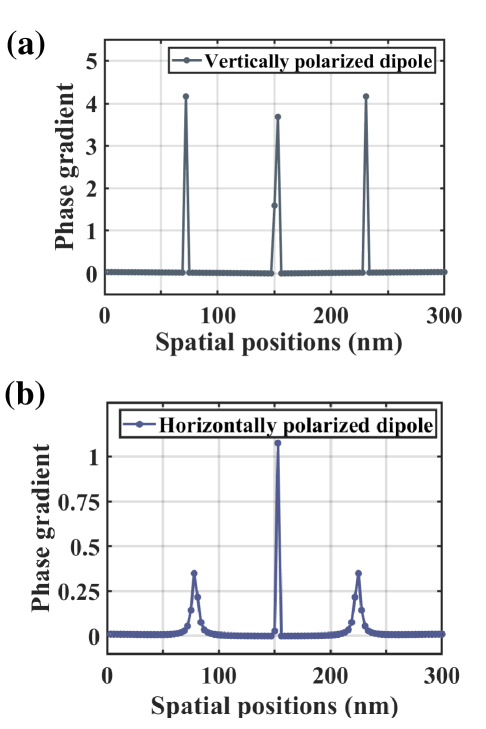
Figure 6: The scattered field phase gradient due to the spatial phase variation within the MSR unit cell for, (a) vertically polarized and (b) horizontally polarized dipole. The spatial dimension covers the length of the MSR unit cell. These results were subtracted w.r.t corresponding results obtained for the planewave excitation. Phase gradients have arbitrary units of length^-1.

III.4 Further discussion of the resonance position of far-field spectra

So far, we have explained the observed resonance redshift and reduction of the resonance linewidth at the far field. However, looking at spectra in Fig.5, it appears contrary to the claim about the frequency shift and also fundamentally challenges the theory. The resonance position doesn’t depend on the dipole source and its polarization. It is an artifact carried out by the simulation setup. Here, we explain that next.
We designed the numerical simulation to obtain the far-field spectra of the MSR at different excitation schemes. This supported comparing results observed in experiments for an MSR device with $\sim 10^{6}$ nanoholes. Therefore, a simulation setup with periodic boundary conditions suffices for the problem, and we need one unit cell of the MSR to simulate. Therefore, the simulation region, along with the field monitor, considers this region as the complete device and projects the corresponding recorded results to the far field. This setup creates the artifact once we shift the MSR excitation. We addressed this issue by calculating the excess spatial phase accumulated in the simulation device due to shifting the source from the planewave to the dipole. That excess spatial phase term is responsible for the change in the apparent far-field resonance position, which can be explained by the perspective of spatiotemporal coupled mode theory.

$$\omega=\omega_{0}+\frac{b}{2}\left(\frac{\partial\phi}{\partial x}\right)^{2}$$ (18)

Equation (18) is brought out of Spatio-Temporal Coupled Mode Theory (STCMT) for non-local metasurfaces [55]; here $x$ represents the spatial dimensions along the MSR plane (chosen as x-y plane), $\phi$ represents the spatial phase of the local scattering field within the MSR nanohole at that plane, and $b$ is the band curvature parameter for the MSR, defined in the supplemental materials [54]. Conventional metasurfaces have extensively used Temporal Coupled Mode Theory (TCMT) to explain the Fano resonance in such structures [56, 57, 58, 59]; however, to understand the effect of spatial dependence, STCMT is needed in MSRs where structural modifications invoke a phase gradient in the far-field scattering response. Here, we have used a conventional MSR, and the simulation device is only a unit cell. That unit cell effectively gets a spatial phase variation at the scattering due to the excitation by a dipole source compared to the planewave [60, 61, 62]. Eq.(18) is defined for a smooth variation of phase $\phi$ over the device space and maps the response in the far field; here, we applied the same idea. First, we measured the smooth variation of the scattering field phase at the MSR unit cell plane, then took its gradient and plotted in Fig.6 for both dipole polarizations. The plotted function in Fig.6 was subtracted w.r.t the phase response of the scattering for the planewave source. Equation 18 assumes the speed of light $c_{0}=1$, thus, $\omega$, $k$ has the unit of length^-1, which is also the unit for $\frac{\partial\phi}{\partial x}$, and $b$ has the unit of length. [55]. Thus, we summed the values of respective gradients, and for $\omega_{0}\equiv\omega_{d}=2.254$ eV, Eq.(18) yields maximum values of the modified resonance frequencies at $2.305$ eV and $2.2676$ eV, for V dipole and H dipole polarizations, respectively, converting back $\omega$ in the unit of frequency (energy). According to the STCMT, these are the far-field resonance positions for our simulated device observing a smooth phase variation over its entire dimension once we shift the source from planewave to embedded dipole. These values explain why we found discrepancies regarding the resonance positions for far-field results in Fig.5. In experiments, however, we need not worry since there the entire device has millions of unit cells. Thus, the local phase gradient in a unit cell becomes insignificant to the far-field objective, which effectively approximates the collected response to a planewave.

IV Conclusions

In summary, this work showed the emergence of the Fano resonance in an all-dielectric GMR-MSR made of an array of nanoholes in high refractive index material, SiN. We took the ab initio theory based on Maxwell’s equations and Feshbach’s formalism to define the Fano interference between the bright and dark modes w.r.t the far field. Then, a multipole moment decomposition was applied to numerically resolve induced moments and their contributions to the local scattering response of the MSR along its plane within the nanohole. Those local scattering responses were recorded by a field monitor coplanar to the MSR plane. The induced ED response was identified as the bright field, and MD and TD responses were identified as dark modes for obvious reasons: fields generated by these moments don’t reach the far field along the outcoupling direction of the MSR, which is along the normal to its plane. Fields from the induced moments MD and TD reach the far-field in the azimuthal directions of the MSR plane, constituting the guided modes. (Details are discussed in the supplemental materials [54].) The main goal of this work was to theoretically identify the effect of the change of the MSR excitation source from the planewave to the dipole embedded in the MSR. We have already applied this in our recent experiment, and there, we saw certain intriguing observations like the resonance redshift, far-field linewidth narrowing, etc. Here, we could define those effects from the ab initio theory and successfully quantify them by numerical calculations using the FDTD simulation. We found that the embedded dipole source offers a stronger scattering response compared to the planewave excitation, and that increases the interference between bright and dark modes. These interference terms were central in controlling all the observables and their numerical values. For the planar symmetry of the MSR, we used parallel dipole polarizations (H dipole) and perpendicular (V dipole) to simulate the MSR. Since dipoles radiate in a perpendicular plane to their polarizations, H dipole radiates in the vertical plane w.r.t the MSR plane. On the other hand, the V dipole radiates along the MSR plane; thus, it couples to the diffractive MSR mode better. This helps the interferences cover all dimensions along the plane, provides a complete solution like a planewave excitation, and retains the asymmetric scattering. H dipole misses on that, although it provides better outcoupling. In the end, we discussed the apparent discrepancy in the far-field resonance position and solved the issue with the help of the STCMT. STCMT is applied on a device capable of showing a smooth spatial phase variation over the dimensions. Our problem concerns the conventional MSR and its far-field spectral properties; TCMT can successfully handle that. Therefore, a simulation device containing one unit cell of the MSR under periodic boundary conditions is the option to solve the problem numerically. Invoking the embedded dipole source showed that it added an extra spatial phase in the simulation device compared to the scattering for the planewave excitation. These get conveyed to the far field following the near-to-far-field relations. We needed to identify the impact of this additional phase. Eq.(18) helped that and found the upper bound of the apparent resonance positions for these spatial phases for each excitation polarization. Since the V dipole covers MSR dimensions completely, it sums more than the H dipole for the spatial phase. These results explain the reason of the apparent discrepancy that could arise from Fig.5.
It is worth noting that we used the STCMT for a unit cell simulation device. To match spectral results with the real MSR device having $\sim 10^{6}$ nanoholes, one option was to design a simulation device with array elements close to this order and maintain simulation step sizes to the present one, which was hardly possible from a computational perspective. Therefore, we had nothing to do but apply the present simulation scheme and correct the resonance frequency outcome as we did. However, one should keep in mind that the real MSR device doesn’t see these phase variations in its far field; compared to their dimensions, these are rapid local phase variations which has no impact, thus, it is not a real, experimental problem.
One can find the application of this numerical investigation for embedded sources rather than only using planewave sources to excite an MSR. Precise tuning of the interference term is key to control observables. Also, this work manifested a GMR-MSR; one can further explore discrete guided modes and their precise control in such devices. The linewidth narrowing effect could be of interest to fundamental studies to investigate subnatural linewidths in the presence of Fano resonance [63, 64].

V Acknowledgement

Authors acknowledge Prof. Girish S. Agarwal, Dept. of Physics and Astronomy, Texas A & M University, for useful discussion and suggestions regarding furnishing the work. J.K.B. acknowledges funding from the Anusandhan National Research Foundation (ANRF), India, through grant number CRG/2021/003026 and DST, FIST grant.

Appendix A Detailed derivation of the results of Electromagnetic theory of Fano resonance

We start from the wave equation obtained from Maxwell’s equation (Derivation is following the references [50, 48, 47]); here, the wave equation is framed with operators and vectors in bra-ket notation,

$$\nabla\times\nabla\times\textbf{E}(\textbf{r},\omega)-\frac{\omega^{2}}{c^{2}\epsilon(\textbf{r},\omega)}\textbf{E}(\textbf{r},\omega)=0$$ (19)

$$\mathcal{M}_{\omega}\textbf{E}(\textbf{r})=\frac{c^{2}}{\epsilon}\nabla\times\nabla\times\textbf{E}(\textbf{r})$$ (20)

$$(\mathcal{M}_{\omega}-\omega^{2}\textbf{I})\ket{\textbf{E}}=0$$ (21)

$$\ket{\textbf{E}}=P\ket{\textbf{E}}+Q\ket{\textbf{E}}$$ (22)

Therefore, Eq.(21) becomes,

$$(\mathcal{M}_{\omega}-\omega^{2}\textbf{I})(P\ket{\textbf{E}}+Q\ket{\textbf{E}})=0$$ (23)

These projection operators, as mentioned in the early works [46, 48, 49], divide the wavefunction into two separate parts; here, these operators are projecting the electric field wavefunction $\ket{\textbf{E}}$ into radiative (bright) and non-radiative (dark) parts. Also, the bright state is a continuum of modes, whereas the dark one is discrete and corresponds to resonances.
Projection operators follow the basic relations,

$$P+Q=I,\quad P^{2}=P,\quad Q^{2}=Q;$$ (24)

Next, Eq.(23) can be written as a set of two coupled equations following Eq.(24);

$$P(\mathcal{M}_{\omega}-\omega^{2}\textbf{I})(P+Q)\ket{\textbf{E}}=0$$ (25)

$$Q(\mathcal{M}_{\omega}-\omega^{2}\textbf{I})(P+Q)\ket{\textbf{E}}=0$$ (26)

Next, Eq.(25) is expanded using the orthogonality condition, $PQ=QP=0$ which readily follows from Eq.(24). Eq.(26) can be expanded in a similar manner.

$$(P\mathcal{M}_{\omega}P-\omega^{2}\textbf{I}P^{2})\ket{\textbf{E}}+P\mathcal{M}_{\omega}Q\ket{\textbf{E}}-\omega^{2}\textbf{I}PQ\ket{\textbf{E}}=0$$

$$\implies(P\mathcal{M}_{\omega}P-\omega^{2}\textbf{I})P\ket{\textbf{E}}=-P\mathcal{M}_{\omega}Q\ket{\textbf{E}}$$

Therefore, the set of the coupled equations become,

$$(P\mathcal{M}_{\omega}P-\omega^{2}\textbf{I})P\ket{\textbf{E}}=-P\mathcal{M}_{\omega}Q\ket{\textbf{E}}$$ (27)

$$(Q\mathcal{M}_{\omega}Q-\omega^{2}\textbf{I})Q\ket{\textbf{E}}=-Q\mathcal{M}_{\omega}P\ket{\textbf{E}}$$ (28)

The discrete non-radiative modes can be expanded as an orthonormal eigenfunction of the corresponding projection operator, i.e., $Q\ket{\textbf{E}_{d}}=\ket{\textbf{E}_{d}}$, therefore it satisfies

$$Q\mathcal{M}_{\omega}Q\ket{\textbf{E}_{d}}=z_{d}^{2}\ket{\textbf{E}_{d}},\quad z_{d}=\omega_{d}+i\gamma_{d}$$ (29)

Where $\omega_{d}$ corresponds to mode resonance frequency and $\gamma_{d}$ goes for intrinsic damping.
Choice of $P$ and $Q$ is such that, asymptotically the bright field projection of $\ket{\textbf{E}}$, i.e., $P\ket{\textbf{E}}$ is identical to the total wavefunction $\ket{\textbf{E}}$, i.e., $P\ket{\textbf{E}}\rightarrow\ket{\textbf{E}}$. Owing to this, the non-radiative projection, $Q\ket{\textbf{E}}$ vanishes asymptotically, and remains in the Hilbert space.
The completeness of $\ket{\textbf{E}_{d}}$ being the eigenfunction of $Q$ asserts,

$$Q=\sum\ket{\textbf{E}_{d}}\bra{\textbf{E}_{d}}$$ (30)

Summation is over the set of discrete eigenfunctions. Equation (28) gives

$$Q\ket{\textbf{E}}=\left(\frac{1}{\omega^{2}-Q\mathcal{M}_{\omega}Q}\right)Q\mathcal{M}_{\omega}P\ket{\textbf{E}}$$ (31)

using this expression in Eq.(27) and expanding that gives,

$$P\mathcal{M}_{\omega}P^{2}\ket{\textbf{E}}-\omega^{2}P\ket{\textbf{E}}+P\mathcal{M}_{\omega}Q\ket{\textbf{E}}=0$$

$$\implies P\mathcal{M}_{\omega}P^{2}\ket{\textbf{E}}-\omega^{2}P\ket{\textbf{E}}+P\mathcal{M}_{\omega}\left(\frac{1}{\omega^{2}-Q\mathcal{M}_{\omega}Q}\right)Q\mathcal{M}_{\omega}P\ket{\textbf{E}}=0$$

$$\implies\left[P\mathcal{M}_{\omega}P+P\mathcal{M}_{\omega}Q\left(\frac{1}{\omega^{2}-Q\mathcal{M}_{\omega}Q}\right)Q\mathcal{M}_{\omega}P-\omega^{2}P\textbf{I}\right]\ket{\textbf{E}}=0$$

Where we have used the identities of Eq.(24). This result summarizes as,

$$(P\mathcal{M}_{\omega}P+V-E)\ket{\textbf{E}}=0,$$ (32)

$$V=P\mathcal{M}_{\omega}Q\left[\frac{1}{(\omega^{2}-Q\mathcal{M}_{\omega}Q)}\right]Q\mathcal{M}_{\omega}P$$ (33)

Resonance appears as the zero of the denominator of the effective potential function $V$; since $Q\mathcal{M}_{\omega}Q\ket{\textbf{E}}=z_{d}^{2}\ket{\textbf{E}}$, $V$ can be divided and expressed in two parts; part for the frequency near the resonance frequency $z_{d}$, and the other part for non-resonant scattering;

$$\left(P\mathcal{M}_{\omega}P+\sum_{\omega^{\prime}\neq\omega_{d}}P\mathcal{M}_{\omega}Q\ket{\textbf{E}^{\prime}}\left[\frac{1}{(\omega^{2}-\omega^{\prime 2})}\right]\bra{\textbf{E}^{\prime}}Q\mathcal{M}_{\omega}P+P\mathcal{M}_{\omega}Q\ket{\textbf{E}_{d}}\left[\frac{1}{(\omega^{2}-z_{d}^{2})}\right]\bra{\textbf{E}_{d}}Q\mathcal{M}_{\omega}P-\omega^{2}P\textbf{I}\right)\ket{\textbf{E}}=0$$ (34)

Here the summation part corresponds to the non-resonant scattering of the field, and the second part involves the resonance, which is discrete in frequency space. Hence, this equation becomes

$$(\mathcal{M^{\prime}}_{\omega}-\omega^{2}\textbf{I})P\ket{\textbf{E}}=-P\mathcal{M}_{\omega}Q\ket{\textbf{E}_{d}}\left[\frac{1}{(\omega^{2}-z_{d}^{2})}\right]\bra{\textbf{E}_{d}}Q\mathcal{M}_{\omega}P\ket{\textbf{E}},$$ (35)

$$\text{where,}\;\;\mathcal{M^{\prime}}_{\omega}=P\mathcal{M}_{\omega}P+\sum_{\omega^{\prime}\neq\omega_{d}}P\mathcal{M}_{\omega}Q\ket{\textbf{E}^{\prime}}\left[\frac{1}{(\omega^{2}-\omega^{\prime 2})}\right]\bra{\textbf{E}^{\prime}}Q\mathcal{M}_{\omega}P$$ (36)

Equation (35) leads to the homogeneous solution of the field wave function satisfying,

$$(\mathcal{M^{\prime}}_{\omega}-\omega^{2}\textbf{I})P\ket{\textbf{E}_{b}}=0$$ (37)

Eq.(37) constructs the dyadic Green’s function $\mathcal{G}_{b}$ which provides the formal solution of Eq.(35);

$$P\ket{\tilde{\textbf{E}}}=P\ket{\textbf{E}_{b}}+\bra{\textbf{E}_{d}}Q\mathcal{M}_{\omega}P\ket{\tilde{\textbf{E}}}\left[\frac{1}{z^{2}_{d}-\omega^{2}}\right]\mathcal{G}_{b}P\mathcal{M}_{\omega}Q\ket{\textbf{E}_{d}}$$ (38)

The asymptotic behaviour of $\ket{\textbf{E}}$ and $\ket{\tilde{\textbf{E}}}$ is different. Their relationship will be discussed later. Now, multiplying $\bra{\textbf{E}_{d}}Q\mathcal{M}_{\omega}P$ from the left of Eq.(38), we get,

$$\bra{\textbf{E}_{d}}Q\mathcal{M}_{\omega}PP\ket{\tilde{\textbf{E}}}=\bra{\textbf{E}_{d}}Q\mathcal{M}_{\omega}PP\ket{\textbf{E}_{b}}+\frac{1}{z^{2}_{d}-\omega^{2}}\bra{\textbf{E}_{d}}Q\mathcal{M}_{\omega}P\mathcal{G}_{b}P\mathcal{M}_{\omega}Q\ket{\textbf{E}_{d}}\bra{\textbf{E}_{d}}Q\mathcal{M}_{\omega}P\ket{\tilde{\textbf{E}}},$$

$$\implies\bra{\textbf{E}_{d}}Q\mathcal{M}_{\omega}P\ket{\tilde{\textbf{E}}}=\bra{\textbf{E}_{d}}Q\mathcal{M}_{\omega}P\ket{\textbf{E}_{b}}+\frac{1}{z^{2}_{d}-\omega^{2}}\bra{\textbf{E}_{d}}Q\mathcal{M}_{\omega}P\mathcal{G}_{b}P\mathcal{M}_{\omega}Q\ket{\textbf{E}_{d}}\bra{\textbf{E}_{d}}Q\mathcal{M}_{\omega}P\ket{\tilde{\textbf{E}}},$$

$$\implies\bra{\textbf{E}_{d}}Q\mathcal{M}_{\omega}P\ket{\tilde{\textbf{E}}}\left(1-\frac{1}{z^{2}_{d}-\omega^{2}}\bra{\textbf{E}_{d}}Q\mathcal{M}_{\omega}P\mathcal{G}_{b}P\mathcal{M}_{\omega}Q\ket{\textbf{E}_{d}}\right)=\bra{\textbf{E}_{d}}Q\mathcal{M}_{\omega}P\ket{\textbf{E}_{b}},$$

$$\implies\bra{\textbf{E}_{d}}Q\mathcal{M}_{\omega}P\ket{\tilde{\textbf{E}}}=\frac{(z^{2}_{d}-\omega^{2})}{z^{2}_{d}-\omega^{2}-\bra{\textbf{E}_{d}}Q\mathcal{M}_{\omega}P\mathcal{G}_{b}P\mathcal{M}_{\omega}Q\ket{\textbf{E}_{d}}}\bra{\textbf{E}_{d}}Q\mathcal{M}_{\omega}P\ket{\textbf{E}_{b}}$$

Putting this last expression in Eq.(38) that can be re-written,

$$P\ket{\tilde{\textbf{E}}}=P\ket{\textbf{E}_{b}}+\frac{\bra{\textbf{E}_{d}}\mathcal{M}_{\omega}P\ket{\textbf{E}_{b}}}{z_{d}^{2}-\omega^{2}-\omega_{d}\Delta}\mathcal{G}_{b}P\mathcal{M}_{\omega}Q\ket{\textbf{E}_{d}},$$ (39)

$$\text{where,}\;\;\Delta=\frac{\bra{\textbf{E}_{d}}\mathcal{M}_{\omega}P\mathcal{G}_{b}P\mathcal{M}_{\omega}\ket{\textbf{E}_{d}}}{\omega_{d}}$$ (40)

Equation(40) is the expression for the resonance shift of resonance position $\omega_{d}$ due to the field overlap between the scattering continuum $P\ket{\textbf{E}_{b}}$ and discrete resonance mode $\ket{\textbf{E}_{d}}$. The negative sign in the denominator of Eq.(39) shows that, there is a red-shift in resonance frequency due to the field coupling of the discrete mode to the mode continuum. Hence, the complete expression for the field $\ket{\tilde{\textbf{E}}}$ can be obtained;

$$\ket{\tilde{\textbf{E}}}=P\ket{\tilde{\textbf{E}}}+Q\ket{\tilde{\textbf{E}}},$$

$$\implies\ket{\tilde{\textbf{E}}}=P\ket{\textbf{E}_{b}}+\frac{\bra{\textbf{E}_{d}}\mathcal{M}_{\omega}P\ket{\textbf{E}_{b}}}{z_{d}^{2}-\omega^{2}-\omega_{d}\Delta}\mathcal{G}_{b}P\mathcal{M}_{\omega}Q\ket{\textbf{E}_{d}}+Q\ket{\tilde{\textbf{E}}}$$

Using Eq.(31), last step above can be expanded further,

$$\ket{\tilde{\textbf{E}}}=P\ket{\textbf{E}_{b}}+\frac{\bra{\textbf{E}_{d}}\mathcal{M}_{\omega}P\ket{\textbf{E}_{b}}}{z_{d}^{2}-\omega^{2}-\omega_{d}\Delta}\mathcal{G}_{b}P\mathcal{M}_{\omega}Q\ket{\textbf{E}_{d}}+\frac{1}{\omega^{2}-z_{d}^{2}}\ket{\textbf{E}_{d}}\bra{\textbf{E}_{d}}\mathcal{M}_{\omega}P\ket{\tilde{\textbf{E}}}$$ (41)

The last term $\bra{\textbf{E}_{d}}\mathcal{M}_{\omega}P\ket{\tilde{\textbf{E}}}$ has been simplified already above, and has been used in Eq.(38) to define Eq.(39). Putting that in Eq.(41) yields,

$$\ket{\tilde{\textbf{E}}}=P\ket{\textbf{E}_{b}}+\frac{\bra{\textbf{E}_{d}}\mathcal{M}_{\omega}P\ket{\textbf{E}_{b}}}{z_{d}^{2}-\omega^{2}-\omega_{d}\Delta}\mathcal{G}_{b}P\mathcal{M}_{\omega}Q\ket{\textbf{E}_{d}}+\frac{(z_{d}^{2}-\omega^{2})}{(\omega^{2}-z_{d}^{2})(z_{d}^{2}-\omega^{2}-\omega_{d}\Delta)}\ket{\textbf{E}_{d}}\bra{\textbf{E}_{d}}\mathcal{M}_{\omega}P\ket{\textbf{E}_{b}},$$

$$\implies\ket{\tilde{\textbf{E}}}=P\ket{\textbf{E}_{b}}+\frac{\bra{\textbf{E}_{d}}\mathcal{M}_{\omega}P\ket{\textbf{E}_{b}}}{z_{d}^{2}-\omega^{2}-\omega_{d}\Delta}\Bigl{(}\mathcal{G}_{b}P\mathcal{M}_{\omega}\ket{\textbf{E}_{d}}-\ket{\textbf{E}_{d}}\Bigr{)}$$ (42)

The dyadic Green’s function $\mathcal{G}_{b}$ of Eq.(37) can be expanded w.r.t $P\ket{\textbf{E}_{b}}$ as orthogonal basis modes [50];

$$\mathcal{G}_{b}=\frac{1}{2\pi}\int d\omega^{\prime}\frac{\ket{P\textbf{E}_{b}(\omega^{\prime})}\bra{P\textbf{E}_{b}(\omega^{\prime})}}{\omega^{{}^{\prime}2}-\omega^{2}}$$ (43)

The integral of this form [Eq.(43)] is solved using complex contour integration as mentioned in Novotny and Hecht’s book [65];

$$\int d\omega^{\prime}\frac{\ket{P\textbf{E}_{b}(\omega^{\prime})}\bra{P\textbf{E}_{b}(\omega^{\prime})}}{\omega^{{}^{\prime}2}-\omega^{2}}=2\pi i\;\text{Res}\left(\frac{\ket{P\textbf{E}_{b}(\omega^{\prime})}\bra{P\textbf{E}_{b}(\omega^{\prime})}}{\omega^{{}^{\prime}2}-\omega^{2}}\right)_{\omega^{\prime}=\omega}$$

$$=\frac{\pi i}{\omega}\ket{P\textbf{E}_{b}(\omega)}\bra{P\textbf{E}_{b}(\omega)}$$

Here, only positive frequency is considered. Hence, Eq.(39) becomes,

$$P\ket{\tilde{\textbf{E}}}=\ket{P\textbf{E}_{b}}+\frac{i}{2\omega}\frac{\bra{\textbf{E}_{d}}\mathcal{M}_{\omega}\ket{P\textbf{E}_{b}}}{z_{d}^{2}-\omega^{2}-\omega_{d}\Delta}\ket{P\textbf{E}_{b}}\bra{P\textbf{E}_{b}}P\mathcal{M}_{\omega}\ket{\textbf{E}_{d}}$$

$$P\ket{\tilde{\textbf{E}}}=\ket{P\textbf{E}_{b}}\left[1+\frac{\left|\bra{\textbf{E}_{d}}\mathcal{M}_{\omega}\ket{P\textbf{E}_{b}}\right|^{2}}{2\omega(z_{d}^{2}-\omega^{2}+\omega_{d}\Delta)}i\right]$$ (44)

Hereon, the intrinsic damping parameter $\Gamma_{i}$ and the resonance width $\Gamma$ are defined;

$$\Gamma_{i}=\frac{\left|\bra{\textbf{E}_{d}}\mathcal{M}_{\omega}\ket{P\textbf{E}_{b}}\right|^{2}\gamma_{d}\omega_{d}}{\omega(z_{d}^{2}-\omega^{2}-\omega_{d}\Delta)^{2}},$$ (45)

$$\Gamma=\frac{\left|\bra{\textbf{E}_{d}}\mathcal{M}_{\omega}\ket{P\textbf{E}_{b}}\right|^{2}}{2\omega(1-\Gamma_{i})},$$ (46)

and the reduced frequency term $\kappa$;

$$\kappa=\frac{\omega^{2}-\omega_{d}^{2}+\omega_{d}\Delta}{\Gamma}$$ (47)

The actual field function $\ket{\textbf{E}}$ should have the same normalization at far field as $\ket{\textbf{E}_{b}}$, hence the relation between $\ket{\textbf{E}}$ and $\ket{\tilde{\textbf{E}}}$ is,

$$\ket{\textbf{E}}=\frac{\cos{\eta\ket{\tilde{\textbf{E}}}}}{(1-\Gamma_{i})}$$ (48)

where,

$$\cot{\eta}=\kappa$$ (49)

with the assumptions $\gamma_{d}\ll\omega_{d}$, and only first order contributions are considered.
Therefore, asymptotically the bright field wave function follows the relation,

$$P\ket{\textbf{E}}=P\ket{\textbf{E}_{b}}\exp{i\eta}$$ (50)

Here $\eta$ is a complex number. The phase of the field wavefunction shifts rapidly by $\sim\pi$ in a frequency range $\Gamma$ around the resonance frequency.
Plots for scattering and far-field spectra having asymmetric resonance are fitted with the following expression defined for Fano resonant scattering;

$$f=f_{0}+h\frac{(\epsilon+q)^{2}}{(1+\epsilon^{2})},\quad\epsilon=\frac{2(E-E_{0})}{\Gamma_{R}}$$ (51)

where $h$ parameterizes the amplitude, $q$ the asymmetry factor, $E_{0}$ is the resonance peak position, and $\Gamma_{R}$ is the usual resonance width obtained with this fit.

References

- Fano [1961] U. Fano, Effects of configuration interaction on intensities and phase shifts, Phys. Rev. 124, 1866 (1961).
- Sarrazin et al. [2003] M. Sarrazin, J.-P. Vigneron, and J.-M. Vigoureux, Role of wood anomalies in optical properties of thin metallic films with a bidimensional array of subwavelength holes, Phys. Rev. B 67, 085415 (2003).
- Maystre [2012] D. Maystre, Theory of wood’s anomalies, in Plasmonics: From Basics to Advanced Topics, edited by S. Enoch and N. Bonod (Springer Berlin Heidelberg, Berlin, Heidelberg, 2012) pp. 39–83.
- Hajebifard and Berini [2017] A. Hajebifard and P. Berini, Fano resonances in plasmonic heptamer nano-hole arrays, Opt. Express 25, 18566 (2017).
- Mousavi et al. [2012] S. H. Mousavi, A. B. Khanikaev, and G. Shvets, Optical properties of fano-resonant metallic metasurfaces on a substrate, Phys. Rev. B 85, 155429 (2012).
- García de Abajo [2007] F. J. García de Abajo, Colloquium: Light scattering by particle and hole arrays, Rev. Mod. Phys. 79, 1267 (2007).
- Fan and Joannopoulos [2002] S. Fan and J. D. Joannopoulos, Analysis of guided resonances in photonic crystal slabs, Phys. Rev. B 65, 235112 (2002).
- Christ et al. [2003] A. Christ, S. G. Tikhodeev, N. A. Gippius, J. Kuhl, and H. Giessen, Waveguide-plasmon polaritons: Strong coupling of photonic and electronic resonances in a metallic photonic crystal slab, Phys. Rev. Lett. 91, 183901 (2003).
- Christ et al. [2008] A. Christ, O. J. F. Martin, Y. Ekinci, N. A. Gippius, and S. G. Tikhodeev, Symmetry breaking in a plasmonic metamaterial at optical wavelength, Nano Letters 8, 2171 (2008).
- Verellen et al. [2009] N. Verellen, Y. Sonnefraud, H. Sobhani, F. Hao, V. V. Moshchalkov, P. V. Dorpe, P. Nordlander, and S. A. Maier, Fano resonances in individual coherent plasmonic nanocavities, Nano Letters 9, 1663 (2009).
- Fan et al. [2010] J. A. Fan, C. Wu, K. Bao, J. Bao, R. Bardhan, N. J. Halas, V. N. Manoharan, P. Nordlander, G. Shvets, and F. Capasso, Self-assembled plasmonic nanoparticle clusters, Science 328, 1135 (2010).
- Luk’yanchuk et al. [2010] B. Luk’yanchuk, N. Zheludev, and S. e. a. Maier, The fano resonance in plasmonic nanostructures and metamaterials., Nature Materials 9, 707–715 (2010).
- Sonnefraud et al. [2010] Y. Sonnefraud, N. Verellen, H. Sobhani, G. A. Vandenbosch, V. V. Moshchalkov, P. Van Dorpe, P. Nordlander, and S. A. Maier, Experimental realization of subradiant, superradiant, and fano resonances in ring/disk plasmonic nanocavities, ACS Nano 4, 1664 (2010).
- Yadav et al. [2020] R. K. Yadav, M. R. Bourgeois, C. Cherqui, X. G. Juarez, W. Wang, T. W. Odom, G. C. Schatz, and J. K. Basu, Room temperature weak-to-strong coupling and the emergence of collective emission from quantum dots coupled to plasmonic arrays, ACS Nano 14, 7347 (2020).
- Yadav et al. [2021] R. K. Yadav, W. Liu, R. Li, T. W. Odom, G. S. Agarwal, and J. K. Basu, Room-temperature coupling of single photon emitting quantum dots to localized and delocalized modes in a plasmonic nanocavity array, ACS Photonics 8, 576 (2021).
- Zhang et al. [2008] S. Zhang, D. A. Genov, Y. Wang, M. Liu, and X. Zhang, Plasmon-induced transparency in metamaterials, Phys. Rev. Lett. 101, 047401 (2008).
- Liu et al. [2009] N. Liu, L. Langguth, and T. e. a. Weiss, Plasmonic analogue of electromagnetically induced transparency at the drude damping limit. nature mater, Nature Materials 8, 758 (2009).
- Liu et al. [2010] N. Liu, T. Weiss, M. Mesch, L. Langguth, U. Eigenthaler, M. Hirscher, C. Sönnichsen, and H. Giessen, Planar metamaterial analogue of electromagnetically induced transparency for plasmonic sensing, Nano Letters 10, 1103 (2010).
- Miroshnichenko et al. [2010] A. E. Miroshnichenko, S. Flach, and Y. S. Kivshar, Fano resonances in nanoscale structures, Rev. Mod. Phys. 82, 2257 (2010).
- Giannini et al. [2011] V. Giannini, Y. Francescato, H. Amrania, C. C. Phillips, and S. A. Maier, Fano resonances in nanoscale plasmonic systems: A parameter-free modeling approach, Nano Letters 11, 2835 (2011).
- Fan et al. [2014] P. Fan, Z. Yu, and S. Fan et al., Optical fano resonance of an individual semiconductor nanostructure., Nature Mater , 471–475 (2014).
- Chen et al. [2018] J. Chen, F. Gan, Y. Wang, and G. Li, Plasmonic sensing and modulation based on fano resonances, Advanced Optical Materials 6, 1701152 (2018).
- Limonov et al. [2017] M. Limonov, M. Rybin, and A. Poddubny et al., Fano resonances in photonics., Nature Photon , 543 (2017).
- Zhang et al. [2018] Y. Zhang, W. Liu, Z. Li, Z. Li, H. Cheng, S. Chen, and J. Tian, High-quality-factor multiple fano resonances for refractive index sensing, Opt. Lett. 43, 1842 (2018).
- Stern et al. [2014] L. Stern, M. Grajower, and U. Levy, Fano resonances and all-optical switching in a resonantly coupled plasmonic–atomic system., Nat Commun 5 (2014).
- Tanaka et al. [2010] K. Tanaka, E. Plum, J. Y. Ou, T. Uchino, and N. I. Zheludev, Multifold enhancement of quantum dot luminescence in plasmonic metamaterials, Phys. Rev. Lett. 105, 227403 (2010).
- Cui et al. [2018] C. Cui, C. Zhou, S. Yuan, X. Qiu, L. Zhu, Y. Wang, Y. Li, J. Song, Q. Huang, Y. Wang, C. Zeng, and J. Xia, Multiple fano resonances in symmetry-breaking silicon metasurface for manipulating light emission, ACS Photonics 5, 4074 (2018).
- Wu et al. [2012] C. Wu, A. Khanikaev, and R. e. a. Adato, Fano-resonant asymmetric metamaterials for ultrasensitive spectroscopy and identification of molecular monolayers., Nature Materials 11, 69–75 (2012).
- Tong et al. [2016] W. Tong, C. Gong, X. Liu, S. Yuan, Q. Huang, J. Xia, and Y. Wang, Enhanced third harmonic generation in a silicon metasurface using trapped mode, Opt. Express 24, 19661 (2016).
- Kroner et al. [2008] M. Kroner, A. Govorov, and S. Remi et al., The nonlinear fano effect., Nature 451, 311–314 (2008).
- Singh et al. [2011] R. Singh, I. A. I. Al-Naib, M. Koch, and W. Zhang, Sharp fano resonances in thz metamaterials, Opt. Express 19, 6312 (2011).
- Kaelberer et al. [2010] T. Kaelberer, V. A. Fedotov, N. Papasimakis, D. P. Tsai, and N. I. Zheludev, Toroidal dipolar response in a metamaterial, Science 330, 1510 (2010).
- He et al. [2018] Y. He, G. Guo, T. Feng, Y. Xu, and A. E. Miroshnichenko, Toroidal dipole bound states in the continuum, Phys. Rev. B 98, 161112 (2018).
- Papasimakis et al. [2016] N. Papasimakis, V. Fedotov, and V. Savinov et al., Electromagnetic toroidal excitations in matter and free space., Nature Mater 15, 263–271 (2016).
- Savinov et al. [2014] V. Savinov, V. A. Fedotov, and N. I. Zheludev, Toroidal dipolar excitation and macroscopic electromagnetic properties of metamaterials, Phys. Rev. B 89, 205112 (2014).
- Zhang et al. [2015] X.-L. Zhang, S. B. Wang, Z. Lin, H.-B. Sun, and C. T. Chan, Optical force on toroidal nanostructures: Toroidal dipole versus renormalized electric dipole, Phys. Rev. A 92, 043804 (2015).
- Zel’Dovich et al. [1958] I. B. Zel’Dovich et al., Electromagnetic interaction with parity violation, Sov. Phys. JETP 6, 1184 (1958).
- Ahmadivand et al. [2017] A. Ahmadivand, B. Gerislioglu, P. Manickam, A. Kaushik, S. Bhansali, M. Nair, and N. Pala, Rapid detection of infectious envelope proteins by magnetoplasmonic toroidal metasensors, ACS Sensors 2, 1359 (2017).
- Liu et al. [2017] G.-D. Liu, X. Zhai, S.-X. Xia, Q. Lin, C.-J. Zhao, and L.-L. Wang, Toroidal resonance based optical modulator employing hybrid graphene-dielectric metasurface, Opt. Express 25, 26045 (2017).
- Gerislioglu et al. [2018] B. Gerislioglu, A. Ahmadivand, and N. Pala, Tunable plasmonic toroidal terahertz metamodulator, Phys. Rev. B 97, 161405 (2018).
- Basharin et al. [2015] A. A. Basharin, M. Kafesaki, E. N. Economou, C. M. Soukoulis, V. A. Fedotov, V. Savinov, and N. I. Zheludev, Dielectric metamaterials with toroidal dipolar response, Phys. Rev. X 5, 011036 (2015).
- Sayanskiy et al. [2018] A. Sayanskiy, M. Danaeifar, P. Kapitanova, and A. E. Miroshnichenko, All-dielectric metalattice with enhanced toroidal dipole response, Advanced Optical Materials 6, 1800302 (2018).
- Xu et al. [2019] S. Xu, A. Sayanskiy, A. S. Kupriianov, V. R. Tuz, P. Kapitanova, H.-B. Sun, W. Han, and Y. S. Kivshar, Experimental observation of toroidal dipole modes in all-dielectric metasurfaces, Advanced Optical Materials 7, 1801166 (2019).
- Zhou et al. [2019] C. Zhou, S. Li, Y. Wang, and M. Zhan, Multiple toroidal dipole fano resonances of asymmetric dielectric nanohole arrays, Phys. Rev. B 100, 195306 (2019).
- Sharma et al. [2024] K. Sharma, D. Rout, A. Nag, V. P, S. K. Selvaraja, G. S. Agarwal, and J. K. Basu, Room temperature emission line narrowing and long-range photon transport in colloidal quantum wells coupled to metasurface resonance, Advanced Optical Materials 12, 2400859 (2024).
- Feshbach [1962] H. Feshbach, A unified theory of nuclear reactions. ii, Annals of Physics 19, 287 (1962).
- Bhatia and Temkin [1984] A. K. Bhatia and A. Temkin, Line-shape parameters for feshbach resonances in he and , Phys. Rev. A 29, 1895 (1984).
- O’Malley and Geltman [1965] T. F. O’Malley and S. Geltman, Compound-atom states for two-electron systems, Phys. Rev. 137, A1344 (1965).
- Hahn et al. [1962] Y. Hahn, T. F. O’Malley, and L. Spruch, Static approximation and bounds on single-channel phase shifts, Phys. Rev. 128, 932 (1962).
- Gallinet and Martin [2011] B. Gallinet and O. J. F. Martin, Ab initio theory of fano resonances in plasmonic nanostructures and metamaterials, Phys. Rev. B 83, 235427 (2011).
- [51] FDTD: 3D Electromagnetic Simulator, Lumerical Inc., https://www.lumerical.com/ansys/.
- Rout et al. [2022] D. Rout, P. Venkatachalam, R. Singh, P. S. Lakshmi, and S. K. Selvaraja, Guided mode resonance aided polarization insensitive in-plane spectral filters for an on-chip spectrometer, Opt. Lett. 47, 4704 (2022).
- Wu et al. [2018] P. C. Wu, C. Y. Liao, V. Savinov, T. L. Chung, W. T. Chen, Y.-W. Huang, P. R. Wu, Y.-H. Chen, A.-Q. Liu, N. I. Zheludev, and D. P. Tsai, Optical anapole metamaterial, ACS Nano 12, 1920 (2018).
- [54] See Supplemental Material at URL-will-be-inserted-by-publisher for the simulation details and additional relevant results.
- Overvig et al. [2024] A. Overvig, S. A. Mann, and A. Alù, Spatio-temporal coupled mode theory for nonlocal metasurfaces., Light Sci Appl. 13 (2024).
- Fan et al. [2003] S. Fan, W. Suh, and J. D. Joannopoulos, Temporal coupled-mode theory for the fano resonance in optical resonators, J. Opt. Soc. Am. A 20, 569 (2003).
- Suh et al. [2004] W. Suh, Z. Wang, and S. Fan, Temporal coupled-mode theory and the presence of non-orthogonal modes in lossless multimode cavities, IEEE Journal of Quantum Electronics 40, 1511 (2004).
- Johnson et al. [2002] S. G. Johnson, P. Bienstman, M. A. Skorobogatiy, M. Ibanescu, E. Lidorikis, and J. D. Joannopoulos, Adiabatic theorem and continuous coupled-mode theory for efficient taper transitions in photonic crystals, Phys. Rev. E 66, 066608 (2002).
- Overvig and Alù [2021] A. Overvig and A. Alù, Wavefront-selective Fano resonant metasurfaces, Advanced Photonics 3, 026002 (2021).
- Rice et al. [2012] E. M. Rice, D. S. Bradshaw, K. Saadi, and D. L. Andrews, Identifying the development in phase and amplitude of dipole and multipole radiation, European Journal of Physics 33, 345 (2012).
- Karedla et al. [2015] N. Karedla, S. C. Stein, D. Hähnel, I. Gregor, A. Chizhik, and J. Enderlein, Simultaneous measurement of the three-dimensional orientation of excitation and emission dipoles, Phys. Rev. Lett. 115, 173002 (2015).
- Nechayev et al. [2019] S. Nechayev, J. S. Eismann, M. Neugebauer, P. Woźniak, A. Bag, G. Leuchs, and P. Banzer, Huygens’ dipole for polarization-controlled nanoscale light routing, Phys. Rev. A 99, 041801 (2019).
- Matthiesen et al. [2012] C. Matthiesen, A. N. Vamivakas, and M. Atatüre, Subnatural linewidth single photons from a quantum dot, Phys. Rev. Lett. 108, 093602 (2012).
- Du et al. [2008] S. Du, P. Kolchin, C. Belthangady, G. Y. Yin, and S. E. Harris, Subnatural linewidth biphotons with controllable temporal length, Phys. Rev. Lett. 100, 183603 (2008).
- Novotny and Hecht [2012] L. Novotny and B. Hecht, Principles of Nano-Optics, 2nd ed. (Cambridge University Press, 2012).