RideAgent: How to Align Operations Research with Taxi Fleet Operators? An LLM-Enhanced Feature-Driven Optimization Framework

Abstract

Taxi pricing and pre-allocation problems are central to urban traffic efficiency and the convenience of residents’ travel. However, previous approaches face challenges in uncertain practical scenarios: (i) unpredictable ride demands due to dynamic factors such as weather and workday variations, and (ii) diverse management objectives of non-expert operators, such as minimizing dispatch costs and enhancing customer satisfaction. This paper introduces RideAgent, a solution tailored for non-expert users, which combines a Large Language Model (LLM) with a feature-driven optimization modeling approach. Experimental results show that RideAgent improves computational efficiency by 53.15% compared to traditional solvers while maintaining an optimality gap of only 2.42%. Furthermore, its variable fixing strategy outperforms five conventional cutting methods, with minimal compromise in solution quality but a significant reduction in computation time of 42.3%. RideAgent effectively caters to personalized operational needs and enables more efficient urban management.

1 Introduction

The electric taxi service is gaining traction in cities and is expected to experience significant growth in the subsequent years. In practice, taxi fleet operators face challenges in mitigating the mismatch between supply and demand, especially during peak hours or in uncertain environments  10.5555/3367032.3367057 . To address the problem, operators can proactively allocate taxis before rush hours, and implement dynamic pricing policies to incentivize taxis traveling to high-demand areas. These two strategies are interdependent, which further complicates the operational problem  zhang2023 . Given the challenges, some operators adopt operations research (OR) tools to support the joint pre-allocation and pricing decision-making process. OR tools refer to decision-making methods based on mathematical models, statistics, and algorithms to optimize complex systems and processes  hillier2015introduction . These techniques are typically used to find the best solutions to problems involving resource allocation, logistics, and other operational challenges. However, conventional OR approaches, such as mixed integer programming (MIP) and dynamic programming (DP), still have some limitations in the development and implementation processes. (i) Limited Data Integration. Traditional approaches struggle with involving covariate features, which may result in biased solutions. (ii) Dynamic and Personalized Objectives. Operators’ evolving and personalized preferences for optimization metrics complicate model formulations. (iii) Knowledge Gaps. Non-expert operators face significant barriers to utilizing professional OR techniques due to the technical complexity of OR tools.

In light of these obstacles, frameworks that integrate Large Language Models (LLMs) with tailored optimization capabilities can effectively tackle these issues by utilizing LLMs’ powerful intent comprehension, reasoning, and tool application abilities  kojima2022large ; shen2024hugginggpt . However, existing LLM-based OR tools focus primarily on natural language understanding and straightforward model invocation  10.24963/ijcai.2024/3 ; ijcai2024p212 , which often compromises the accuracy of modeling based on user questions and leads to biased solutions. For example, after prompt optimization, in a small-scale traveling salesman problem with 50 nodes, GPT-4 achieves an optimal GAP of 11%  yang2023large ; achiam2023gpt . These biases can manifest as suboptimal or even infeasible pre-allocation and pricing strategies. Furthermore, the intricate interdependence of joint strategies, coupled with the inherent uncertainties of the taxi system, poses significant challenges in solving complex OR models in a short time  Kamga2013HailingIT . These limitations highlight the need to improve the accuracy and efficiency of the LLM-guided decision-making process.

To tackle the above issues, we propose RideAgent, a novel LLM-guided variable fixing strategy tailored for non-expert users, integrated with a feature-driven optimization modeling approach. Our contributions are as follows.

• Feature-Driven Optimization Integration with LLM Agent for Taxi System. In order to further account for environmental uncertainties and covariates, RideAgent incorporates a feature-driven optimization framework that integrates a random forest (RF) with an optimization model. This framework allows for the inclusion of numerous features, thereby enhancing the alignment with user requirements and reducing decision-making bias.

• LLM-Guided Variable Fixing Strategy for Enhanced Optimization. We introduce a novel variable fixing strategy guided by LLMs’ reasoning ability. Based on limited historical optimal decision data, RideAgent can learn the rules of optimal decision-making and reasonably parameterize a part of decision variables with small contributions to the optimal solution. By focusing on key variables, this approach simplifies the pre-defined large-scale optimization problem and enhances the computational efficiency.

• Real-World Case Study Validation of LLM-Driven Optimization. We validate the effectiveness of RideAgent through a comprehensive real-world case study. Results demonstrate that RideAgent excels in generating accurate objective functions to accommodate user requirements. Benchmarking against the full-scale MIP model, RideAgent shows superior performance in computational time and solution quality across different parameterization scales. Comparison with existing methods highlights the potential of applying LLM-based OR tools in smart city operations.

The remainder of this paper is organized as follows: Section 2 reviews some related work. Section 3 defines the optimization models. Section 4 introduces the structure and functions of RideAgent. Section 5 analyzes the results of the case study. Section 6 summarizes our work.

2 Related Work

2.1 Joint Vehicle Pre-Allocation and Pricing

The joint vehicle pre-allocation and pricing problem has attracted attention in the transportation literature. The intrinsic fluctuations of service demand introduce complexity to the decision-making framework  ozkan2020joint . Conventional deterministic optimization models do not account for dynamic changes, which may result in biased solutions. To address these challenges, an increasing number of researchers have adopted various optimization approaches to account for spatiotemporal uncertainty in service demand and enhance decision-making effectiveness. Existing studies propose stochastic or robust optimization models  xu2018electric ; pantuso2022exact ; EJOR2024 or dynamic programming models  shah2022joint ; chen2023real , and then use reformulation techniques, heuristic algorithms or approximation algorithms to derive efficient solutions.

Existing research often overlooks the impact of covariate features on uncertainty and struggles to incorporate features into OR models  hao2020robust . Additionally, the complexity of the joint strategy necessitates OR expertise, which may limit its wider application to non-expert groups. To bridge these gaps, we integrate OR models with LLMs to provide more accessible and responsible solutions.

2.2 LLM-Assisted OR Tools

LLMs utilize deep learning techniques and become promising tools for supporting various human tasks. LLMs have also been explored in the realm of OR applications, with two primary approaches: (1) LLMs as Optimizers utilize in-context learning  dong2022survey ; nie2024importance to conduct optimization through conversational interfaces and leverage chain of thought (CoT) prompts  kojima2022large to harness reasoning capabilities. In this way, LLMs as optimizers do not require specialized OR knowledge. (2) LLM Agents are capable of generating optimization models via callable APIs  chacon2024large ; xu2024large . Recent studies propose integrating OR with LLMs in agents and mainly focus on deterministic MIP models  li2023large ; ahmaditeshnizi2023optimus .

Nevertheless, existing LLM-based OR techniques exhibit limitations in accuracy and efficiency. LLMs as optimizers sometimes are difficult to guarantee the accuracy of solutions for some complex problems  yang2023large . In addition, LLM agents are generally restricted to dealing with simple and well-defined problems.

2.3 Feature-Driven Optimization

LLM agents have limitations in dealing with various practical problems in uncertain environments. The feature-driven optimization framework outputs decisions directly from input covariates. We identify three feature-driven paradigms for learning policies, namely, decision rule optimization, sequential learning and optimization, and integrated learning and optimization  review2024 . In our proposed agent, we extend the approach of Biggs et al. ((Biggs_2022, )) and integrate the prediction and optimization processes. Specifically, we utilize a pre-trained RF to incorporate more covariate features in the uncertain urban taxi system. In this way, the framework can better cope with diverse user queries.

3 Problem Formulation

3.1 Joint Vehicle Pre-Allocation and Pricing Model

Electric taxis provide services throughout cities, and taxi stops can be clustered into different areas. During the rush hours, such as 8-9 am, the demand for taxis varies greatly from area to area, while the number of parked taxis is relatively uniform. This will cause a shortage of taxis in some areas, while there will be idle taxis in other areas, resulting in resource waste and user dissatisfaction. Electric taxis have $|K|$ different states of charge (SOC) where $K=\left\{1,...,|K|\right\}$ is the set of discretized SOC. The demand for vehicles with lower SOC can be met by vehicles with higher SOC, but not vice versa.

Define the set of supply areas as $I=\left\{1,...,|I|\right\}$ and the set of demand areas as $J=\left\{1,...,|J|\right\}$. Operators allocate unoccupied vehicles from $|I|$ supply areas to $|J|$ demand areas with supply shortage $z_{jk}$ before rush hours, which is defined as the extra number of vehicles with SOC $k$ required to fulfill the demand in area $j,j\in J$. Let $S_{ik}$ denote the number of idle vehicles with SOC $k$ at supply area $i,i\in I$.

Following earlier papers  10.1145/3178876.3186134 ; hao2020robust , we assume that the average taxi fare per order $\hat{u}_{jk}$ is related to the departure area $j$ and SOC $k$, and is affected by the total demand for taxis with SOC $k$. The pre-allocation cost of each vehicle $w_{ij}=\hat{w}_{ij}+b_{j}$, where $\hat{w}_{ij}$ is the inconvenience cost and $b_{j}$ is the online booking fee. Operators pay an inconvenience cost $\hat{w}_{ij}$ for a driver allocated from supply area $i$ to demand area $j$, and $\hat{w}_{ij}$ is proportional to the distance between areas. Operators pay the booking fee $b_{j}$ for each driver who is allocated to demand area $j$, and the booking fee will be paid by the passenger when there is a successful pick-up. Define $\theta$ ($0\leq\theta\leq 1$) as the fixed share for operators, which means operators earn $\theta*100\%$ of each taxi order. Operators earn average revenue $u_{jk}$ per order for vehicles with SOC $k$: $u_{jk}=\theta*\hat{u}_{jk}+b_{j}$. Operators need to decide $x_{ijk}$, the number of taxis with SOC $k$ to be allocated from supply area $i$ to demand area $j$. At the same time, operators need to decide the average fare per order $\hat{u}_{jk}$ for SOC $k$ in demand area $j$. Define $d_{jk}$ as the number of demands of SOC $k$ that are satisfied in demand area $j$. The operating income is the order revenue in demand areas: $R(\mathbf{u},\mathbf{d})=\sum_{j\in J}\sum_{k\in K}u_{jk}d_{jk}$. The operating cost is the taxi pre-allocation cost: $C(\mathbf{x})=\sum_{j\in J}\sum_{i\in I}\sum_{k\in K}w_{ij}x_{ijk}$. The goal is to maximize the operational profit: $R(\mathbf{u},\mathbf{d})-C(\mathbf{x})$.

Based on these definitions, we formulate the electric taxi pre-allocation and pricing optimization model as follows:

$$\max\limits_{\mathbf{x},\mathbf{u},\mathbf{v},\mathbf{d}}\quad R(\mathbf{u},\mathbf{d})-C(\mathbf{x})$$ (1)

s.t. $$\sum_{j\in J}x_{ijk}\leq S_{ik},\forall i\in I,k\in K,$$ (2)

$$d_{jk}=z_{jk}\wedge\big{[}\sum_{i\in I}x_{ijk}+v_{j(k+1)}\big{]},\forall j\in J,k\in K,$$ (3)

$$v_{jk}=\big{[}\sum_{i\in I}x_{ijk}-z_{jk}+v_{j(k+1)}\big{]}^{+},\forall j\in J,k\in K,$$ (4)

$$v_{jk}=0,\forall k\notin K,$$ (5)

$$x_{ijk}\in\mathbb{N},\forall i\in I,j\in J,k\in K$$ (6)

Objective (1) represents the total operational profit from vehicle pre-allocation and pricing decisions. Constraint (2) means that the total number of vehicles of each SOC allocated a supply area does not exceed the number of its existing vehicles. Constraint (3) indicates that the number of user demands actually met in each demand area is the minimum value between user demands and the number of vehicles with sufficient SOC. Constraint (4) represents the number of vehicles remaining for each SOC after meeting user demands. Constraint (5) limits the boundary conditions, and constraint (6) represents that the number of pre-allocated vehicles is a non-negative integer.

3.2 RF-based Feature-Driven Model

Deterministic models are generally ineffective because external factors have a significant impact on user demands. Therefore, we introduce a RF-based feature-driven model, which can make full use of historical operation data and explore the relationship between system features (such as weather and operation decisions) and operation results (profit). The tree structure also augments LLM’s reasoning process. In addition, the feature-driven structure can achieve direct prediction from decisions to targets, reducing the accumulation of random parameter prediction errors.

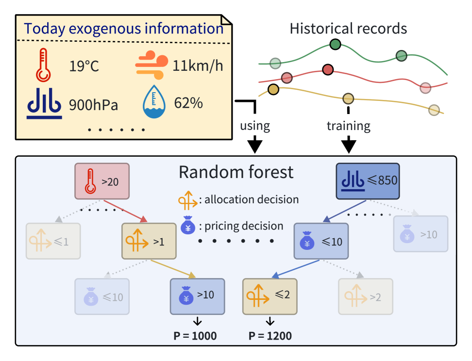
Figure 1: A Sample Tree of the Trained RF After Variable Fixing

We illustrate a sample tree of RF in Figure 1. RF is trained using the historical exogenous features data (weather and day of the week) and operational records. Suppose there are $|H|$ trees in the RF, and the leaf node of each tree $h$ represents the predicted operational profit $P(\mathbf{y},\mathbf{c})$, where $\mathbf{y}=(\mathbf{x},\mathbf{u})$ is the decision variable and $\mathbf{c}$ is the feature. Our goal is to maximize the operation profit by maximizing $P(\mathbf{y},\mathbf{c})$. Let $N^{h}$ denote the number of nodes (excluding the leaves) in tree $h$. For each interior node $n$, let $p_{n},l_{n}$ and $r_{n}$ be the immediate parent, the left and right children, respectively. Let $L^{h}$ represent the set of leaves in tree $h$, and let $P_{m}^{h}\;(m\in L^{h})$ denote the score of each leaf. Given the trained RF, we introduce binary variables $q_{n_{1},n_{2}}^{h}$ to select branches and decide the range of the variables. The corresponding $0\text{-}1$ MIP model is as follows:

$$\max\limits_{\mathbf{y},\mathbf{q}}\quad \frac{1}{|H|}\sum_{h=1}^{|H|}\sum_{m\in L^{h}}P_{m}^{h}q_{p_{m},m}^{h}$$ (7)

s.t. $$a_{n,h}\mathbf{y}-M\left(1-q_{n,l_{n}}^{h}\right)\leq b_{n}^{h},\forall h\in H,n\in N^{h},$$ (8)

$$a_{n,h}\mathbf{y}+M\left(1-q_{n,r_{n}}^{h}\right)\geq b_{n}^{h},\forall h\in H,n\in N^{h},$$ (9)

$$q_{n,l_{n}}^{h}+q_{n,r_{n}}^{h}=q_{p_{n},n}^{h},\forall h\in H,n\in N^{h},$$ (10)

$$\sum_{n\in L^{h}}q_{p_{n},n}^{h}=1,\forall h\in H,$$ (11)

$$q_{n,l_{n}}^{h},q_{n,r_{n}}^{h},q_{p_{n},n}^{h}\in\{0,1\},\forall h\in H,n\in N^{h},$$ (12)

$$\text{Constraints}\;(\ref{con1})\text{-}(\ref{con5}).$$

Objective (7) is to maximize the predicted profit, that is to maximize the score of the selected leaves. Constraint (8) and constraint (9) are big-M logical constraints to determine which leaf the solution $\mathbf{y}$ lies in. Constraint (10) ensures that if a parent node is inactive, its children must also be inactive; but if any child is active, then the parent must also be active. Constraint (11) guarantees that within each tree $h$, only one leaf can be active. Constraint (12) defines the binary variables. According to the basic vehicle pre-allocation and pricing model, constraints (2)-(6) still need to be satisfied to ensure that the solution obtained is also feasible for the original problem.

3.3 LLM-embedded Feature-Driven Model

After receiving and analyzing the user’s question, the LLM agent will convert the user’s question text into the target function code that can be run in the solver. Then, the LLM agent will identify the decision variables $\mathbf{y}^{\prime}$ that contribute the least to the optimal solution, and then fix the chosen decision variables with the mean values of the historical optimal value $\bar{\mathbf{y}}^{\prime}$. $\hat{\textbf{y}}=\textbf{y}\backslash\textbf{y}^{\prime}$. This model refinement process is achieved by employing a prompted $\textbf{LLM}(Q;\mathcal{D},P^{\text{PP}})$, relying on the user’s query $Q$, empirical records $\mathcal{D}$ and prompt $P^{\text{PP}}$  salemi2024optimization . The LLM agent is described in detail in the next section.

Define $A(\mathbf{c})F(\mathbf{y})\leq K(\mathbf{c})$ to depict the feasible region and constraints related to $\mathbf{y}$. After reducing the scope of the RF-based model by fixing some decision variables, we have the following optimization problem:

$$\max\limits_{\hat{\mathbf{y}},\mathbf{q}}\quad \frac{1}{|H|}\sum_{h=1}^{|H|}\sum_{m\in L^{h}}P_{m}^{h}q_{p_{m},m}^{h}$$ (13)

$$\min_{\hat{\mathbf{y}},\mathbf{q}}\quad \textbf{LLM}(Q;\mathcal{D},P^{\text{PP}})$$ (14)

s.t. $$A(\mathbf{c})F(\hat{\mathbf{y}},\bar{\mathbf{y}}^{\prime})\leq K(\mathbf{c}),$$ (15)

$$\text{Constraints}\;(\ref{con21})\text{-}(\ref{con25}).$$

Objective (14) is generated by the LLM agent based on the user’s query $Q$, and is less prioritized than objective (13). Constraint (15) represents constraints for selecting branches of the trees, parameterizing a portion of the operational decision variables. Constraints (8)-(12) involve binary variables to explain branch and leaf selection in RF.

After parameterizing some redundant variables $\textbf{y}^{\prime}$, RideAgent offers a more agile model, especially notable for its reduced computation time.

4 LLM-based Agent

This section introduces the structure of our proposed agent and its various functions. The macro structure of the agent adopts a process similar to human cooperation and decision-making, and adds some tricks in specific functions to adapt to the vehicle pre-allocation and pricing problem  wei2022chain ; xiao2023chain . A visual representation of the agent framework is provided in Figure 2. Please refer to Appendix A.2 for the detailed pseudocode of the agent implementation process.

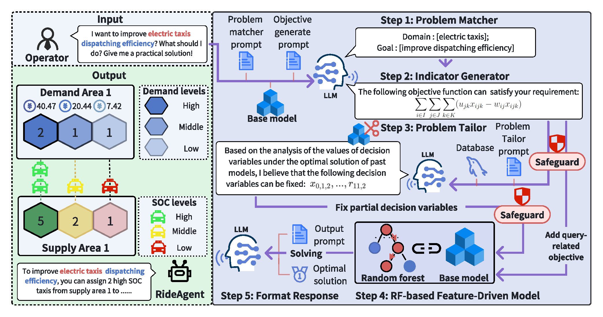
Figure 2: The agent framework

Step 1: Problem Matcher. Users submit a natural language (NL) query $Q$ focused on a particular objective within a defined region (e.g., How to improve the electric taxi dispatching efficiency?). Such a query is then analyzed by Problem Matcher (see Figure 2 Step 1) to identify an appropriate domain-specific agent (e.g., electric taxis).

Step 2: Indicator Generator. The indicator generator (see Figure 2 Step 2) formulates NL queries $Q$ into a convex indicator function $f(\textbf{y};\textbf{w})$ based on operation decisions y (e.g., number of allocated electric taxis and average order price for high SOC vehicles) and parameters w in the feature-driven programming.

$$f(\textbf{y};\textbf{w})=\textbf{LLM}(Q;P^{\text{IG}}):\mathbb{R}^{|\mathcal{Y}|\times|\mathcal{W}|}\rightarrow\mathbb{R}_{+},$$ (16)

where $P^{\text{IG}}$ denotes the predefined prompts and $\mathcal{Y},\mathcal{W}$ denote the feasible domain of decision variables y and set of parameters w, respectively. The indicator function $f(\textbf{y};\textbf{w})$ is then integrated into the objective of MIP for re-optimization purposes. Furthermore, the retrievable historical operational database $\mathcal{D}$ is available in the form of an API that generates Structured Query Language (SQL) by an LLM. Metric $S$ is established to evaluate the extent to which the query $Q$ is satisfied. Subsequently, Code Safeguard scrutinizes the output code of $f(\textbf{y};\textbf{w})$ to ensure compliance with the coding standards required by solvers like Gurobi and CPLEX  he2024can .

Step 3: Problem Tailor. The role of Problem Tailor is to distill the broad queries $Q$ into more focused decisions subsets $\hat{\textbf{y}}$ and to identify the pertinent factors. Problem Tailor initiates by utilizing SQL commands generated by the LLM to extract relevant information from the database $\mathcal{D}$, which contains rich historical taxi operational data and a small amount of historical optimal decisions that maximize operating profits. Problem Tailor then assesses which operational decisions contribute the least to the optimal solutions and subsequently retains the most relevant decision variables $\hat{\textbf{y}}$. This methodology can be encapsulated within a minimization framework:

$$\hat{\textbf{y}}_{t}=\arg\ \min_{\textbf{y}\in\mathcal{Y}}\textbf{LLM}(Q;\mathcal{D},P_{t}^{\text{PP}}(\hat{\textbf{y}}_{t-1},S_{t-1})),$$ (17)

where the prompt $P_{t}^{\text{PP}}(\hat{\textbf{y}}_{t-1},S_{t-1})$ in iteration $t$ contains previously selected variables $\hat{\textbf{y}}_{t-1}$ and satisfaction factor $S_{t-1}=\frac{|(f(\hat{\textbf{y}}^{*}_{t-1},\textbf{y}^{\prime};\textbf{w})-f(\hat{\textbf{y}};\textbf{w})|}{f(\hat{\textbf{y}};\textbf{w})}$. This framework enables the LLM to evaluate the most pertinent decision variables $\hat{\textbf{y}}$ and strive for an enhanced $S_{t}$ value. For ease of implementation, $\textbf{y}^{\prime}$ is aligned with average historical optimal data points $\textbf{y}^{\text{hist}}$ and is represented as equivalent constraints in subsequent steps. After that, Code Safeguard reviews the constraints generated by the LLM to ensure they adhere to the syntax requirements of optimization solvers.

Step 4: RF-based Feature-Driven Model. The RF-based feature-driven model $\min_{\textbf{y}\in\mathcal{Y}}g(\textbf{y},\textbf{w})$ (see details in the previous section) consists of two components (Figure 2 Step 4): (i) Pre-trained RF, tailored to a particular urban optimization goal (taxi operation profits), functions as a predictive analytics tool. (ii) MIP: Drawing on previous research  Biggs_2022 , the structure of the RF is embedded within an MIP model. The MIP’s objectives encompass operational targets as well as indicators related to the query $f(\textbf{y};\textbf{w})$ supplied by Indicator Generator. Furthermore, the parameterized variables $\textbf{y}^{\prime}$, presented as equality constraints, are integrated into the MIP constraints. Subsequently, the agent proceeds to optimize the problem that yields a more focused decision subset:

$$\hat{\textbf{y}}^{*}_{t}=\arg\min_{\hat{\textbf{y}}}g(\hat{\textbf{y}};\bar{\textbf{y}}^{\prime},\textbf{w}).$$ (18)

Fixing irrelevant decisions concerning $Q$, the reduced scope model $\min_{\hat{\textbf{y}}}g(\hat{\textbf{y}};\bar{\textbf{y}}^{\prime},\textbf{w})$ efficiently yields high quality solutions $\hat{\textbf{y}}^{*}_{t}$ within reduced computational time.

Step 5: Response Prompter. The feature-driven model iteratively generates optimal solutions, aiming to fulfill the user’s query as assessed by the indicator metrics. The iterative process terminates when the satisfaction factor exceeds a threshold and remains stable across subsequent iterations. Finally, Response Prompter translates the optimal solutions and associated scores $(\textbf{y}^{*},S^{*})$ into a format that is more accessible and understandable for the end users.

5 Case Study

In this section, we conduct a case study using real-world taxi trip data. Numerical experiments demonstrate the multiple capabilities of RideAgent.

5.1 Dataset Description

Experiments are conducted using New York City yellow taxi trip records in 2016  nyctripdataset . The trip records of New York yellow taxis include information such as the start and end time and location of trips. Since the trip records do not include real-time counts of taxis parked in each area and historical operation decisions, we use a reasonable strategy to simulate and generate this part of data. The weather data of New York City in 2016 comes from Kaggle  weatherdataset . We randomly select morning peak periods of 14 days and use Gurobi solver to obtain the optimal decisions that maximize the operating profit (obj 13). These optimal decisions are input to the agent as small sample optimal decision data.

5.2 Experimental Settings

We conduct three experiments, focusing on the accuracy of indicator generation and the efficiency of model solving. In all experiments, we adopt the unit-test methodology to evaluate the effectiveness of the RideAgent  li2023large . The unit-test methodology, inspired by software development practices, evaluates individual components of a system by running multiple experiments with distinct test questions.

Taxi fleet operators need to consider the concerns of other stakeholders when making decisions. To make the experiments more comprehensive, we add two other representative perspectives when generating indicators: passengers and city managers. For each perspective, we design a series of 6 queries, 5 of which can be formulated as linear objective functions, and the remaining one needs to be formulated as a nonlinear objective function. The relevant objective function of each query is accompanied by a correct answer verified by human annotators (Further details in Appendix A.3). Given the potential variability of LLM’s output  casper2023open , we execute each query 10 times for linear objective functions, and subsequently average the accuracy and efficiency metrics. We solve mathematical optimization models using Gurobi 10.

5.3 Experiment Results

5.3.1 Tests on the Accuracy of Objective Function Generation

To demonstrate the validity of the generated objective function, we execute accuracy tests by assessing the similarity between the objective functions generated by RideAgent and human-annotated standard objective functions. Sometimes the code of two functions may diverge, but their underlying mathematical significance could be the same. To address this problem, we introduce two metrics based on the Jaro-Winkler distance algorithm: text similarity and result similarity. These metrics quantify the similarity between the “generated objective function” and the “standard objective function” concerning their codes and mathematical essence, respectively (see Appendix A.4 for details).

• The term “Prompts” refers to the number of standard objective functions used in each experiment.

Prompts¹ In-sample test Out-of-sample test Result similarity Text similarity Result similarity Text similarity 0 —— —— 0.72 0.86 5 0.85 0.94 0.79 0.90 10 0.89 0.95 0.81 0.91 15 0.93 0.96 —— ——

Table 1: Accuracy Test Results for Linear Objectives

Prompts¹ In-sample test Out-of-sample test Result similarity Text similarity Result similarity Text similarity 0 —— —— 0.71 0.86 1 0.81 0.94 0.75 0.85 2 0.83 0.95 0.78 0.84 3 0.83 0.96 —— ——

Table 2: Accuracy Test Results for Nonlinear Objectives

Tables 1 and 2 show that RideAgent performs well in the out-of-sample test where no standard answer is given in the prompt ($0$ prompt), and the text similarity of both linear and non-linear indicator functions reaches 86%. As the number of “Prompts” increases, it can be observed that the similarity between the generated objective and the standard objective functions gradually increases in both in-sample and out-of-sample tests. The results indicate that RideAgent utilizes the generalization ability of LLMs to formulate objectives that are closely related to user queries. The results also show that the hallucination problem when LLMs are applied to objective function generation can be alleviated by adding expert knowledge to the prompts.

5.3.2 Tests on the Efficiency of Model Solving

We test several existing LLM-assisted OR tools and are unable to solve the joint taxi pre-allocation and pricing optimization problem studied in this paper. OptiMUS ahmaditeshnizi2023optimus fails to generate a reasonable mathematical model. ORPO yang2023large struggles to obtain high-quality solutions for large-scale problems involving uncertainty. While OptiGuide li2023large is effective for supply chain operations, it cannot be applied to taxi operations. All of these tools lack the capability to integrate rich historical data and produce reliable solutions.

Existing LLM-assisted OR tools enhance the interaction with users but are weak in solution accuracy. When facing large-scale models, Rideagents can achieve higher solving efficiency compared to precise solution methods. The baseline model, mentioned as “FULL”, is the full-scale LLM-embedded feature-driven model without decision variables fixing. The model proposed by RideAgent and the FULL model share identical objectives, including operational profit objectives (labeled as “RF-Obj”) and additional query-relevant objectives (labeled as “QR-Obj”) in each experiment. The number of “Prompts” is fixed to 8. Define the metric “Parameterized scale” as the number of decision variables fixed by RideAgent. Tables 3 and 4 record the efficiency test results for linear and nonlinear objectives respectively. The “time gap” refers to the time saved by using RideAgent. The “optimization gap” refers to the gap between the solution obtained by Rideagent and the global optimal solution obtained by solving the FULL model. For both linear and nonlinear objectives, the results show that the CPU time of RideAgent is about 53.15% shorter than FULL on average. The RF-Obj Gap and the QR-Obj Gap are as small as 0.78% and 4.05% on average. It means that RideAgent has higher solving efficiency than the FULL model, and strikes a balance between solution optimality and solving time.

Parameterized Scale	In-sample				Out-of-sample
	RideAgent			Gurobi	RideAgent			Gurobi
	OptimizationGAP(%)		CPU time (s)	CPU time (s)	OptimizationGAP(%)		CPU time (s)	CPU time (s)
	RF-Obj gap	QR-Obj Gap			RF-Obj Gap	QR-Obj Gap
[0-50]	0.41	1.73	65.19	120.07	0.57	2.68	99.76	150.81
[50-100]	1.23	1.31	15.81	96.16	1.10	5.78	102.02	159.34
[100-150]	1.17	0.05	16.69	85.75	1.20	5.78	66.51	156.51
[150-250]	1.61	2.07	19.42	111.21	1.47	3.82	38.08	128.68

Table 3: Results of the Efficiency Test for Linear Objectives

Parameterized Scale	Dispatching efficiency				Market share				Supply-demand matching degree
	CPU time(s)		RF-Obj Gap(%)	QR-Obj Gap(%)	CPU time(s)		RF-Obj Gap(%)	QR-Obj Gap(%)	CPU time(s)		RF-Obj Gap(%)	QR-Obj Gap(%)
	Agent	FULL			Agent	FULL			Agent	FULL
10%	144.20	1092.92	0.96	8.72	100.82	200.66	0.88	13.63	56.01	170.87	0.88	4.03
20%	56.07	1125.23	1.55	18.51	59.18	199.66	1.55	18.48	31.88	168.71	1.55	2.58
30%	34.49	1126.86	1.72	36.66	31.78	199.23	1.73	36.60	17.14	166.43	1.72	3.90

Table 4: Results of the Efficiency Test for Nonlinear Objectives

Cuts Name	In sample			Out of sample
	Time Gap	RF-Obj Gap	QR-Obj Gap	Time Gap	RF-Obj Gap	QR-Obj Gap
CliqueCuts atamturk2000conflict	39.46s(30.49%)	0.80%	5.13%	50.75s(42.58%)	1.08%	5.30%
CoverCuts ceria1998cutting	43.18s(33.09%)	0.80%	5.13%	55.44s(46.75%)	1.08%	5.09%
GomoryCuts gomory2010outline	53.00s(43.01%)	0.80%	5.26%	62.33s(52.48%)	1.08%	4.97%
GUBCoverCuts wolsey1990valid	46.45s(36.80%)	0.80%	5.18%	59.35s(49.94%)	1.08%	5.02%
MIRCuts marchand2001aggregation	46.56s(36.46%)	0.80%	5.13%	61.31s(51.65%)	1.08%	5.27%
Total average	45.73s(35.97%)	0.80%	5.16%	57.83s(48.68%)	1.08%	5.13%

Table 5: Comparison Results with Cutting Methods

In Efficiency Test for Linear Query-Relevant Objectives, RideAgent’s parameterized scale varies across experiments. The experimental results are divided into four intervals based on the number of fixed variables. For linear QR-Obj, two objective gaps are shown in Figures 3 (a) and (b) respectively. As shown in Figure 3 and Table 3, as the parameterized scale increases, the gap between the objectives tends to increase and becomes unstable. Figure 3 (c) shows the time reduction for solving the model proposed by RideAgent. The computational time reduction of groups in-sample and out-of-sample is similar, while the solution suboptimality of in-sample group is lower. Thus, providing the agent with standard objective functions improves optimization reliability.

In Efficiency Test for Nonlinear Query-Relevant Objectives, we experiment on three nonlinear QR-Obj, namely dispatching efficiency, market share, and supply-demand matching degree. Since the time cost of nonlinear objectives is high, we fix the parameterized scale at 10%, 20%, and 30% of the total number of operational decisions (1032). Five experiments are conducted for each query. As can be seen from Table 4, for nonlinear query-relevant objective functions, as the variable fixing scale increases, the suboptimality of RF-Obj remains low (1.39% on average) and increases slightly, while the suboptimality of QR-Obj increases significantly. This is because the historical optimal decision we give to the agent is only for RF-Obj, and the law learned by the agent may conflict with QR-Obj. When the agent optimizes nonlinear user QR-Obj, the advantage of model solving time is more prominent (shortened by 80.08% on average).

5.3.3 Test on Comparison with Cutting Methods

We compare the LLM-guided variable fixing strategy with five commonly used cuts (CliqueCuts, CoverCuts, GomoryPassesCuts, GUBCoverCuts, MIRCuts). Similar to the previous experiments, the number of prompts is fixed to 8, and the experiments are conducted in-sample and out-of-sample, with each repeated five times. Since nonlinear objective functions are inconvenient to compare the quality of solutions, only linear query-relevant objectives are used in this experiment. For experiments of a type of cut, this type of cut is turned off during solving, and RideAgent parameterizes a part of decision variables. Table 5 records the mean values of experimental results with different cuts disabled. According to Table 5, the variable fixing strategy implemented in RideAgent is more effective than five conventional cuts, with only minor sacrifice in solution quality (0.94% and 5.15%) but a significant reduction in computation time by 51.78s (42.32%). For more complex and time-consuming MIP models and even nonlinear programming, RideAgent is expected to achieve a significant improvement in computational efficiency.

6 Conclusion

In this paper, we propose RideAgent, an LLM agent designed to address the challenges inherent in taxi pricing and pre-allocation. By combining the powerful capabilities of LLMs with feature-driven optimization methods, RideAgent meets the flexible needs of non-expert operators and improves practical applicability. Case studies show that RideAgent can generate reliable query-relevant objective functions, and has better computational efficiency and lower global suboptimality when compared with solving the full-scale model. In addition, its variable fixing strategy exhibits superior performance compared to conventional cutting methods. These findings suggest that RideAgent provides a promising solution to real-world urban transportation problems.

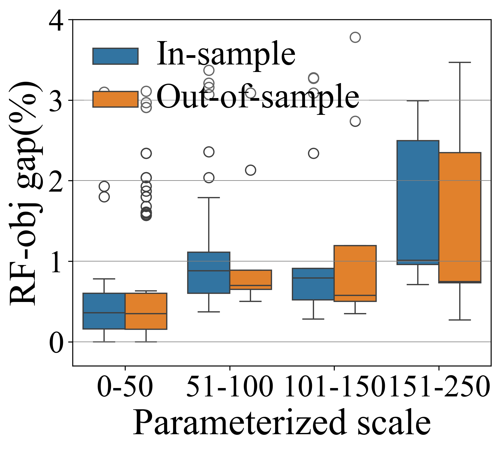
(a) RF-obj Gaps

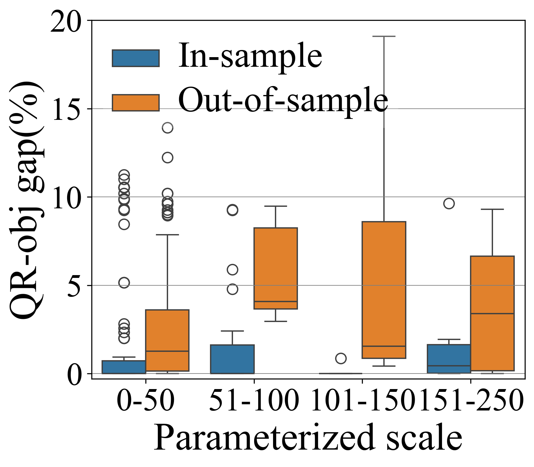
(b) QR-obj Gaps

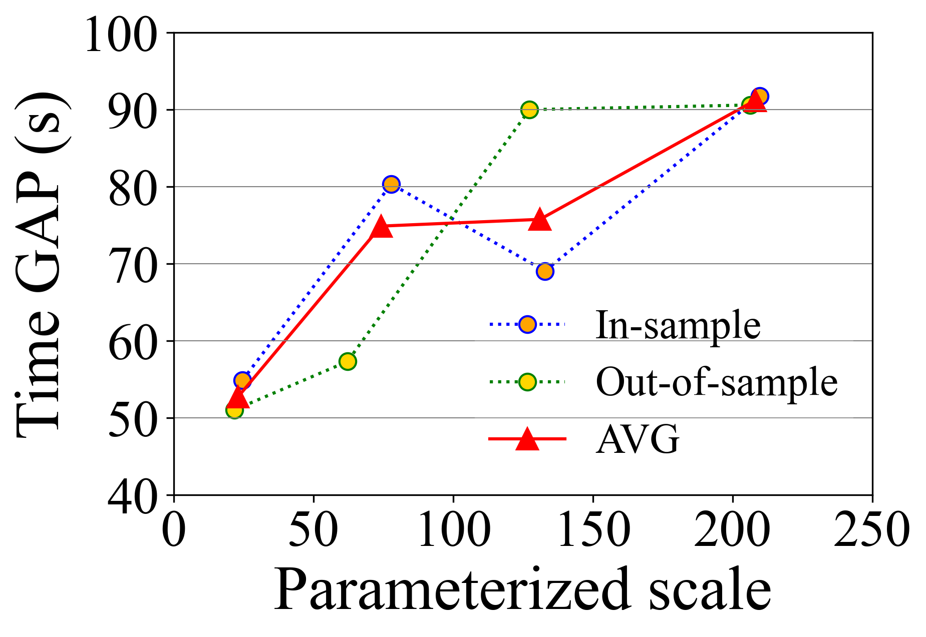
(c) Reduced Solving Time by Agent

Figure 3: Efficiency Test Results for Linear Objectives

Appendix A Appendix

A.1 Detailed Experimental Settings

We cluster all the pick-up and drop-off stops in the taxi trip records into 50 areas based on their geographical locations. The morning peak time is defined as 8:00 a.m. to 8:30 a.m. According to the historical trip records and the simulation results of regional vehicle inventory, it can be found that the vehicle demand in the morning peak time in 8 areas is not fully met by the regional vehicle inventory, while the remaining 42 areas have idle vehicles. They are defined as demand and supply areas respectively.

The inconvenience cost $\hat{w}_{ij}$ is calculated as $0.5 per kilometer. The fixed share for operators $\theta$ is set at $0.2 and the online booking fee $b_{j}=\$5$. Assume that electric vehicles have three discrete power levels: low, medium, and high, corresponding to SOC of 0, 1, and 2 respectively.

The data used to train the RF are the morning peak operation data and exogenous features of 366 days in 2016. In the RF, the number of trees is 200 and the maximum depth is limited to 150. 30% of the data is used as a test set. The RF achieves an accuracy of 93.4% and 60.7% on the training set and test set, respectively.

All experiments are run on a macOS system equipped with an Apple M1 Pro CPU and 16GB of RAM. See the Appendix A.1 for detailed experimental settings

Utilizing GPT-4o mini, we establish the agent framework leveraging Langchain, a standard framework for creating applications powered by LLMs.

A.2 Pseudocode

The pseudocode outlined in Algorithm 1 delineates the workflow of RideAgent, which is tailored to handle user queries within an urban operations management framework.

The input includes the NL user query $Q$, an initial empty set $\textbf{y}^{\prime}_{0}$ of parameterized decisions, and satisfaction score $S_{0}$ initialized to zero, along with the LLM prompts $P^{\text{IG}}$ and $P^{\text{PP}}(\textbf{y}^{\prime}_{0},S_{0})$. Initially, Problem Matcher pinpoints an agent that aligns with the query’s context. Subsequently, Indicator Generator activates, fulfilling three roles: it formulates a query-specific indicator function $f(\textbf{y};\textbf{w})$ using the LLM, it calculates a satisfaction metric $S_{t}$.

The iterative cycle then initiates, sustained by a condition that persists until the iteration limit is reached or the satisfaction metric remains above zero. During each iteration, Problem Tailor retrieves empirical data related to decisions $\mathcal{D}$ from the database and refines the LLM-Optimal parameterized decisions $\textbf{y}^{\prime}_{t}$. The algorithm then addresses a RF-based feature-driven model $\min_{\textbf{y}\in\mathcal{Y}}g(\textbf{y};\textbf{w})$ with the objective function $f$. It narrows the solution space and revises both the satisfaction score $S_{t}$ and the LLM prompts $P^{\text{PP}}(\textbf{y}^{\prime}_{0},S_{0})$ for subsequent iterations.

Upon meeting the convergence criteria or the termination conditions, the algorithm delivers the optimized decision vector $\textbf{y}^{*}$ along with the ultimate satisfaction score $S^{*}$, signifying the end of optimization process led by RideAgent.

Algorithm 1 RideAgent pseudocode

0: Query $Q$, initial value $S_{0}=0$, LLM prompts $P^{\text{IG}},P_{0}^{\text{PP}}(\textbf{y}^{\prime}_{0},S_{0})$.

 Problem Matcher: Determine an area-specific agent.

 Indicator Generator:

   1. Query-relevant indicator function $f(\textbf{y};\textbf{w})=\textbf{LLM}(Q;P^{\text{IG}})$ generation.

   2. Objective $f(\textbf{y};\textbf{w})$ code generation (code safeguard checked).

   3. Satisfaction factor $S_{t}=\frac{|(f(\hat{\textbf{y}}^{*}_{t};\bar{\textbf{y}}^{\prime},\textbf{w})-f(\bar{\textbf{y}};\textbf{w})|}{f(\bar{\textbf{y}};\textbf{w})}$ generation.

 while $\{t\leq\text{max-iterations}\}$ or $\{S_{t}>0\}$ do

  a. Problem Tailor:

    1. Call decision-related empirical data $\mathcal{D}=(\bar{\textbf{y}},\bar{\textbf{w}})$ from a database.

    2. Update the LLM-Optimal parameterized decisions $\textbf{y}^{\prime}_{t}$: $\textbf{y}^{\prime}_{t+1}=\arg\ \max_{\textbf{y}\in\mathcal{Y}}\textbf{LLM}(Q;\mathcal{D},P_{t}^{\text{PP}}(\textbf{y}^{\prime}_{t},S_{t})),$

  b. Solve a $f$ objective embedded feature-driven model $g(\textbf{y};\textbf{w})$:

    1. Optimal Scoping down solutions: $\hat{\textbf{y}}^{*}_{t+1}=\arg\min_{\hat{\textbf{y}}}g(\hat{\textbf{y}};\bar{\textbf{y}}^{\prime}_{t+1},\textbf{w}),$

    2. Update $S_{t+1},P_{t+1}^{\text{PP}}(\textbf{y}^{\prime}_{t+1},S_{t+1})$.

    return $\hat{\textbf{y}}^{*}_{t+1},S_{t+1}$.

 end while

 return  $\left\{\textbf{y}^{*}\right\}\left\{S^{*}\right\}$.

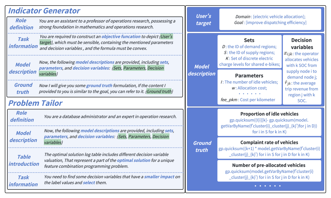
Figure 4: Brief introduction of prompt

A.3 Objective Function Standard Answer

In this section, we provide the ground-truth Q&A instructions adopted in the prompt of RideAgent. Specifically, we provide accurate Q&A information (human-labeled) in three specific scenarios: Operational, Customer-Related, and Regulatory. These scenarios encompass the majority of operational inquiries proposed by taxi fleet operators. Within each scenario, there are typically 3 to 8 key QR-objs that are of utmost relevance to the majority of taxi fleet operators (as shown in Table 6). For each QR-obj, we provide a ground-truth “Answers” that is derived from human experience. This information is supplied in the form of a Gurobi objective code.

A.4 Objective Function Similarity Index

This section presents the mathematical representation of the Gurobi code created by RideAgent, which is utilized to quantify the “Results Similarity” in the relevance test. The Gurobi code is shown below, which represents the objective of maximizing the total number of accessible e-bikes and its related mathematical essence:

• Gurobi code: model.setObjective( gp.quicksum(model.getVarByName( f"cluster{i}_cluster{j}_{k}") for i in S for j in D for k in K), GRB.MAXIMIZE)

• Mathematical essence: $\max\ \hat{u}_{0,0}+\hat{u}_{0,1}+\hat{u}_{0,2}+\underbrace{\quad\quad\quad\quad\cdots\cdots\quad\quad\quad\quad}_{\hat{u}_{j,k}\ for\ j\ in\ [4,7,12,15,37,38,44]\ for\ k\ in\ [0,1,2]}+\hat{u}_{49,0}+\hat{u}_{49,1}+\hat{u}_{49,2}$

• Gurobi code: model.setObjective( gp.quicksum(model.getVarByName( f"cluster{i}_cluster{j}_{k}") for i in S for j in D for k in K if k >0), GRB.MAXIMIZE)

• Mathematical essence: $\max\ \hat{u}_{0,1}+\hat{u}_{0,2}+\underbrace{\quad\quad\quad\quad\cdots\cdots\quad\quad\quad\quad}_{\hat{u}_{j,k}\ for\ j\ in\ [4,7,12,15,37,38,44]\ for\ k\ in\ [0,1,2]}+\hat{u}_{49,1}+\hat{u}_{49,2}$

A.5 Prompt

Figure 4 shows the prompts input to the LLMs for two parts of the agent, Indicator Generator and Problem Tailor. These prompts contain role definitions, task descriptions, and valid problem information.

Table 6: Ground-truth objectives

Scenario QR-obj Ground-truth Obj-code Operations Proportion of idle vehicles $\mathtt{model.setObjective(gp.quicksum((I[i][k]-gp.quicksum(model.getVarByName(f^{\prime}cluster\{i\}\_cluster\{j\}\_\{k\}^{\prime})forjinD))foriinSforkinK),}$ $\mathtt{GRB.MINIMIZE)}$ Idle vehicles cost $\mathtt{model.setObjective(gp.quicksum((k+1)*(I[i][k]-gp.quicksum(model.getVarByName(f^{\prime}cluster\{i\}\_cluster\{j\}\_\{k\}^{\prime})forjinD))}$ $\mathtt{foriinSforkinK),GRB.MINIMIZE)}$ Number of high-powered taxis in demand areas $\mathtt{model.setObjective(gp.quicksum(model.getVarByName(f^{\prime}cluster\{i\}\_cluster\{j\}\_2^{\prime})foriinSforjinD),GRB.MAXIMIZE)}$ Future service Level of vehicles $\mathtt{model.setObjective(gp.quicksum(k*model.getVarByName(f^{\prime}cluster\{i\}\_cluster\{j\}\_\{k\}^{\prime})foriinSforjinDforkinK),GRB.MAXIMIZE)}$ Scheduled vehicle response time $\mathtt{model.setObjective(gp.quicksum(model.getVarByName(f^{\prime}cluster\{i\}\_cluster\{j\}\_\{k\}^{\prime})*d[i][j]foriinSforjinDforkinK),GRB.MINIMIZE)}$ Dispatching efficiency of vehicles $\mathtt{model.setObjective(gp.quicksum(model.getVarByName(f^{\prime}avg_{r}eward\{j\}\_\{k\}^{\prime})*model.getVarByName(f^{\prime}cluster\{i\}\_cluster\{j\}\_\{k\}^{\prime})}$ $\mathtt{-w[i][j]*model.getVarByName(f^{\prime}cluster\{i\}\_cluster\{j\}\_\{k\}^{\prime})foriinSforjinDforkinK),GRB.MAXIMIZE)}$ customer Complaint rate of vehicles $\mathtt{model.setObjective(gp.quicksum((k+1)*model.getVarByName(f^{\prime}cluster\{i\}\_cluster\{j\}\_\{k\}^{\prime})foriinSforjinDforkinK),GRB.MAXIMIZE)}$ Service Level of vehicles $\mathtt{model.setObjective(gp.quicksum(model.getVarByName(f^{\prime}cluster\{i\}\_cluster\{j\}\_\{k\}^{\prime})*(k+1)foriinSforjinDforkinK),GRB.MAXIMIZE)}$ Average travel price of vehicles $\mathtt{model.setObjective(gp.quicksum(model.getVarByName(f^{\prime}avg_{r}eward\{j\}\_\{k\}^{\prime})forjinDforkinK),GRB.MINIMIZE)}$ Order completion rate of vehicles $\mathtt{model.setObjective(gp.quicksum((k+1)*model.getVarByName(f^{\prime}cluster\{i\}\_cluster\{j\}\_\{k\}^{\prime})foriinSforjinDforkinK),GRB.MAXIMIZE)}$ Average waiting time of vehicles $\mathtt{model.setObjective(gp.quicksum(model.getVarByName(f^{\prime}cluster\{i\}\_cluster\{j\}\_\{k\}^{\prime})*d[i][j]foriinSforjinDforkinK),GRB.MINIMIZE))}$ Supply-demand matching degree of vehicles $\mathtt{model.setObjective(gp.quicksum(gp.quicksum(I[i][k]-gp.quicksum(model.getVarByName(f^{\prime}cluster\{i\}\_cluster\{j\}\_\{k\}^{\prime})}$ $\mathtt{forjinD)forkinK)foriinS)+gp.quicksum(abs(demand_{a}vg[j]-inventory_{a}vg-}$ $\mathtt{gp.quicksum(model.getVarByName(f^{\prime}cluster\{i\}\_cluster\{j\}\_\{k\}^{\prime})foriinSforkinK))forjinD),GRB.MINIMIZE)}$ Regulatory Number of pre-allocated vehicles $\mathtt{model.setObjective(gp.quicksum(model.getVarByName(f^{\prime}cluster\{i\}\_cluster\{j\}\_\{k\}^{\prime})foriinSforjinDforkinK),GRB.MAXIMIZE)}$ Average passenger capacity of vehicles $\mathtt{model.setObjective(gp.quicksum((k+1)*model.getVarByName(f^{\prime}cluster\{i\}\_cluster\{j\}\_\{k\}^{\prime})foriinSforjinDforkinK),GRB.MAXIMIZE)}$ Number of users covered by vehicles $\mathtt{model.setObjective(gp.quicksum((k+1)*model.getVarByName(f"cluster\{i\}\_cluster\{j\}\_\{k\}")foriinSforjinDforkinK),GRB.MAXIMIZE)}$ User satisfaction of vehicles $\mathtt{model.setObjective(gp.quicksum(model.getVarByName(f^{\prime}cluster\{i\}\_cluster\{j\}\_\{k\}^{\prime})*(k+1)foriinSforjinDforkinK),GRB.MAXIMIZE)}$ Demand satisfaction rate $\mathtt{model.setObjective(gp.quicksum((k+1)*model.getVarByName(f"cluster\{i\}\_cluster\{j\}\_\{k\}")foriinSforjinDforkinK),GRB.MAXIMIZE)}$ Market share of vehicles $\mathtt{model.setObjective(gp.quicksum(model.getVarByName(f^{\prime}avg_{r}eward\{j\}\_\{k\}^{\prime})*model.getVarByName(f^{\prime}cluster\{i\}\_cluster\{j\}\_\{k\}^{\prime})}$ $\mathtt{foriinSforjinDforkinK),GRB.MAXIMIZE)}$

References

- [1] Josh Achiam, Steven Adler, Sandhini Agarwal, Lama Ahmad, Ilge Akkaya, Florencia Leoni Aleman, Diogo Almeida, Janko Altenschmidt, Sam Altman, Shyamal Anadkat, et al. Gpt-4 technical report. arXiv preprint arXiv:2303.08774, 2023.
- [2] Ali AhmadiTeshnizi, Wenzhi Gao, and Madeleine Udell. Optimus: Optimization modeling using mip solvers and large language models. arXiv preprint arXiv:2310.06116, 2023.
- [3] Alper Atamtürk, George L Nemhauser, and Martin WP Savelsbergh. Conflict graphs in solving integer programming problems. European Journal of Operational Research, 121(1):40–55, 2000.
- [4] Max Biggs, Rim Hariss, and Georgia Perakis. Constrained optimization of objective functions determined from random forests. Production and Operations Management, 32(2):397–415, 2022.
- [5] Stephen Casper, Xander Davies, Claudia Shi, Thomas Krendl Gilbert, Jérémy Scheurer, Javier Rando, Rachel Freedman, Tomasz Korbak, David Lindner, Pedro Freire, et al. Open problems and fundamental limitations of reinforcement learning from human feedback. arXiv preprint arXiv:2307.15217, 2023.
- [6] Sebastian Ceria, Cécile Cordier, Hugues Marchand, and Laurence A Wolsey. Cutting planes for integer programs with general integer variables. Mathematical programming, 81:201–214, 1998.
- [7] Camilo Chacón Sartori, Christian Blum, and Gabriela Ochoa. Large language models for the automated analysis of optimization algorithms. In Proceedings of the Genetic and Evolutionary Computation Conference, pages 160–168, 2024.
- [8] Guangyao Chen, Siwei Dong, Yu Shu, Ge Zhang, Jaward Sesay, Börje Karlsson, Jie Fu, and Yemin Shi. Autoagents: a framework for automatic agent generation. In Proceedings of the Thirty-Third International Joint Conference on Artificial Intelligence, IJCAI ’24, 2024.
- [9] Mengjing Chen, Weiran Shen, Pingzhong Tang, and Song Zuo. Dispatching through pricing: modeling ride-sharing and designing dynamic prices. In Proceedings of the 28th International Joint Conference on Artificial Intelligence, IJCAI’19, page 165–171, 2019.
- [10] Qi Chen, Yanzhe Lei, and Stefanus Jasin. Real-time spatial–intertemporal pricing and relocation in a ride-hailing network: Near-optimal policies and the value of dynamic pricing. Operations Research, 2023.
- [11] Qingxiu Dong, Lei Li, Damai Dai, Ce Zheng, Zhiyong Wu, Baobao Chang, Xu Sun, Jingjing Xu, and Zhifang Sui. A survey for in-context learning. arXiv preprint arXiv:2301.00234, 2022.
- [12] Ulrik Eilertsen, Olav M Falck-Pedersen, Jone V Henriksen, Kjetil Fagerholt, and Giovanni Pantuso. Joint relocation and pricing in electric car-sharing systems. European Journal of Operational Research, 315(2):553–566, 2024.
- [13] Ralph E Gomory. Outline of an algorithm for integer solutions to linear programs and an algorithm for the mixed integer problem. Springer, 2010.
- [14] Zhaowei Hao, Long He, Zhenyu Hu, and Jun Jiang. Robust vehicle pre-allocation with uncertain covariates. Production and Operations Management, 29(4):955–972, 2020.
- [15] Qianyu He, Jie Zeng, Wenhao Huang, Lina Chen, Jin Xiao, Qianxi He, Xunzhe Zhou, Jiaqing Liang, and Yanghua Xiao. Can large language models understand real-world complex instructions? In Proceedings of the AAAI Conference on Artificial Intelligence, volume 38, pages 18188–18196, 2024.
- [16] Frederick S Hillier and Gerald J Lieberman. Introduction to operations research. McGraw-Hill, 2015.
- [17] Shan Jiang, Le Chen, Alan Mislove, and Christo Wilson. On ridesharing competition and accessibility: Evidence from uber, lyft, and taxi. In Proceedings of the 2018 World Wide Web Conference, WWW ’18, page 863–872, Republic and Canton of Geneva, CHE, 2018. International World Wide Web Conferences Steering Committee.
- [18] Kaggle. New york city taxi trip - hourly weather data. https://www.kaggle.com/datasets/meinertsen/new-york-city-taxi-trip-hourly-weather-data, 2017.
- [19] Camille Kamga, M. Anil Yazici, and Abhishek Singhal. Hailing in the rain: Temporal and weather-related variations in taxi ridership and taxi demand-supply equilibrium. 2013.
- [20] Takeshi Kojima, Shixiang Shane Gu, Machel Reid, Yutaka Matsuo, and Yusuke Iwasawa. Large language models are zero-shot reasoners. Advances in neural information processing systems, 35:22199–22213, 2022.
- [21] Beibin Li, Konstantina Mellou, Bo Zhang, Jeevan Pathuri, and Ishai Menache. Large language models for supply chain optimization. arXiv preprint arXiv:2307.03875, 2023.
- [22] Hugues Marchand and Laurence A Wolsey. Aggregation and mixed integer rounding to solve mips. Operations research, 49(3):363–371, 2001.
- [23] Younes Mechqrane, Christian Bessiere, and Ismail Elabbassi. Using large language models to improve query-based constraint acquisition. In Proceedings of the Thirty-Third International Joint Conference on Artificial Intelligence, IJCAI-24, pages 1916–1925, 2024.
- [24] Allen Nie, Ching-An Cheng, Andrey Kolobov, and Adith Swaminathan. The importance of directional feedback for llm-based optimizers. arXiv preprint arXiv:2405.16434, 2024.
- [25] Erhun Özkan. Joint pricing and matching in ride-sharing systems. European Journal of Operational Research, 287(3):1149–1160, 2020.
- [26] Giovanni Pantuso. Exact solutions to a carsharing pricing and relocation problem under uncertainty. Computers & Operations Research, 144:105802, 2022.
- [27] Alireza Salemi, Surya Kallumadi, and Hamed Zamani. Optimization methods for personalizing large language models through retrieval augmentation. In Proceedings of the 47th International ACM SIGIR Conference on Research and Development in Information Retrieval, pages 752–762, 2024.
- [28] Sanket Shah, Meghna Lowalekar, and Pradeep Varakantham. Joint pricing and matching for city-scale ride-pooling. In Proceedings of the International Conference on Automated Planning and Scheduling, volume 32, pages 499–507, 2022.
- [29] Yongliang Shen, Kaitao Song, Xu Tan, Dongsheng Li, Weiming Lu, and Yueting Zhuang. Hugginggpt: Solving ai tasks with chatgpt and its friends in hugging face. Advances in Neural Information Processing Systems, 36, 2024.
- [30] Taxi & Limousine Commission. Tlc trip record data. https://www.nyc.gov/site/tlc/about/tlc-trip-record-data.page, 2024.
- [31] Sadana Utsav, Abhilash Chenreddy, Erick Delage, Alexandre Forel, Emma Frejinger, and Thibaut Vidal. A survey of contextual optimization methods for decision-making under uncertainty. European Journal of Operational Research, 2024.
- [32] Jason Wei, Xuezhi Wang, Dale Schuurmans, Maarten Bosma, Fei Xia, Ed Chi, Quoc V Le, Denny Zhou, et al. Chain-of-thought prompting elicits reasoning in large language models. Advances in neural information processing systems, 35:24824–24837, 2022.
- [33] Laurence A Wolsey. Valid inequalities for 0–1 knapsacks and mips with generalised upper bound constraints. Discrete Applied Mathematics, 29(2-3):251–261, 1990.
- [34] Ziyang Xiao, Dongxiang Zhang, Yangjun Wu, Lilin Xu, Yuan Jessica Wang, Xiongwei Han, Xiaojin Fu, Tao Zhong, Jia Zeng, Mingli Song, et al. Chain-of-experts: When llms meet complex operations research problems. In The Twelfth International Conference on Learning Representations, 2023.
- [35] Jinglue Xu, Jialong Li, Zhen Liu, Nagar Anthel Venkatesh Suryanarayanan, Guoyuan Zhou, Jia Guo, Hitoshi Iba, and Kenji Tei. Large language models synergize with automated machine learning. arXiv preprint arXiv:2405.03727, 2024.
- [36] Min Xu, Qiang Meng, and Zhiyuan Liu. Electric vehicle fleet size and trip pricing for one-way carsharing services considering vehicle relocation and personnel assignment. Transportation Research Part B: Methodological, 111:60–82, 2018.
- [37] Chengrun Yang, Xuezhi Wang, Yifeng Lu, Hanxiao Liu, Quoc V Le, Denny Zhou, and Xinyun Chen. Large language models as optimizers. arXiv preprint arXiv:2309.03409, 2023.
- [38] Xianjie Zhang, Pradeep Varakantham, and Hao Jiang. Future aware pricing and matching for sustainable on-demand ride pooling. In Proceedings of the AAAI Conference on Artificial Intelligence, volume 37, pages 14628–14636, 2023.