The Generalized Uncertainty Principle. New Bounds and Trends

Abstract

The Heisenberg uncertainty principle is one of the fundamental pillars of quantum mechanics and quantum field theory. It is normally introduced by postulating the commutation relations $[\hat{x}^{i},\hat{p}^{j}]=i\hbar\delta^{ij}$. However, as suggested by some quantum gravity models and string theory, this basic principle no longer holds true in the presence of a minimal length, possible the Plank length, and modifications of the commutation have been proposed i.e., of the form $[\hat{x}^{\mu},\hat{p}^{\nu}]=-i\hbar(1+\beta_{0}\,\hat{p}^{2}/\Lambda^{2})\eta^{\mu\nu}$(plus possible additional terms). In this work we will consider the previous modified uncertainty principle in terms of an effective field theory, comment upon some theoretical subtleties that are often overlooked in the literature, and constrain , for the first time, the $\Lambda$ scale with the Compton high-energy experimental data. Our findings suggest that high-energy experiments are potentially sensitive to these corrections and could serve as an effective framework for probing possible violations of the Heisenberg uncertainty principle.

1 Introduction

The Generalized Uncertainty Principle (GUP) was first introduced by Maggiore:1993kv ; Kempf_1995 ; Scardigli_1999 and extensively analyzed in later studies Bang:2006va ; Bosso:2023aht ; Pedram:2011aa ; Galan:2007ns ; Das:2012rv ; Pedram:2011gw ; Mignemi:2011wh ; Nozari:2012gd ; Tedesco:2011iv ; Balasubramanian:2014pba ; Tkachuk:2013lta ; Bosso:2022vlz ; Pramanik:2013zy ; Bosso:2018uus ; Chung:2018btu ; Bosso:2020fos ; Bosso:2020jay ; Scardigli_1999 ; Hossenfelder_2006 ; Das_2016 ; Maccone_2014 ; Tawfik_2014 ; Hossenfelder_2013 ; Nenmeli_2021 ; Chen_2013 ; Basilakos_2010 ; Gecim_2017 ; Gecim_2018 ; KONISHI1990276 ; Chang_2011 ; Gomes_2022 ; Das_2008 ; ali ; Marin . It normally appears in quantum gravity models Scardigli_1999 ; Hossenfelder_2013 ; Basilakos_2010 ; Gecim_2018 ; Das_2008 ; ali ; Marin and string theory KONISHI1990276 ; Chang_2011 ; Hossenfelder:2012jw and is a consequence of the presence of a minimal length, which is usually associated with the Planck length. The GUP is mathematically introduced by modifying the standard commutation relations with additional terms, i.e.,

$$[\hat{x}^{\mu},\hat{p}^{\nu}]=-i\eta^{\mu\nu}(1+\beta\hat{p}^{2}+...)+\gamma\,\hat{p}^{\mu}\hat{p}^{\nu}+...\,,$$ (1)

in natural units, where $\beta$ and $\gamma$ can be re expressed as

$$\beta=\frac{\beta_{0}}{\Lambda^{2}}\,\qquad\gamma=\frac{\gamma_{0}}{\Lambda^{2}}\,,$$ (2)

with dimensionless constants $\beta_{0}$ and $\gamma_{0}$, and $\Lambda$, the energy scale where the GUP becomes relevant. As mentioned previously, $\Lambda$ is normally considered on the Planck scale, and therefore all current high-energy and precision experiments are, at least in principle, insensitive to the presence of these new terms. However, it is legitimate to consider extensions of the Heisenberg principle regardless of its original motivation from quantum gravity or string theory. Even if it constitutes one of the building blocks of modern physics, it has not yet been probed with high-energy experiments within an effective field theory framework, which is the main goal of our paper.

In the previously mentioned analyses both relativistic and non-relativistic formulations of GUP have been studied, and some collaborations obtained bounds on the $\beta_{0}/\Lambda^{2}$ terms within non-relativistic models, or from astrophysical data. These experimental bounds are nicely summarized in Bosso:2023aht . The strongest bound is given by $\beta^{-1/2}=\beta_{0}^{-1/2}\Lambda>10$ Tev, within a non-relativistic and anisotropic framework Gomes_2022

$$[\hat{x}_{i},\hat{p}_{j}]=i\hbar\left[f(\hat{\mathbf{p}})\delta_{ij}+g_{i}(\hat{\mathbf{p}})\hat{p}_{j}\right].$$ (3)

However, these bounds are not directly applicable to our analysis as the previous model is non-relativistic and the deformed commuting relations are different from the ones employed in our analysis. All other bounds are weaker by a few orders of magnitude. Thus, in this manuscript, we derive a precise bound on $\beta$ using high-energy experimental data.

The manuscript is organized as follows. In the first part, we present the theoretical framework, emphasizing the differences with previous approaches. The second part is devoted to the derivation of the leading-order modified QED Lagrangian induced by the GUP, along with the corresponding Feynman rules. We then carry out a phenomenological analysis based on high-energy Compton scattering data Achard_2005 . Finally, we summarize our findings and conclusions.

2 Preliminary considerations

Many authors have previously performed calculations within the relativistic GUP framework in quantum field theory using different approaches for the calculations of the physical cross sections and other observables Hossenfelder:2012jw ; Bosso:2020fos ; Bosso:2020jay ; Hossenfelder:2004up ; Quesne:2006is ; Kober:2010sj ; Kober:2011dn ; Husain:2012im ; Faizal:2017map . However, the method employed in this manuscript present some differences with previous works, and all the explicit technical details will be given in this section.

Let us start with the standard commutation relations that can be expressed in covariant form as

$$[\hat{x}^{\mu},\hat{p}^{\nu}] =-i\eta^{\mu\nu}\,,$$ (4)

$$[\hat{p}^{\mu},\hat{p}^{\nu}] =[\hat{x}^{\mu},\hat{x}^{\nu}]=0\,,$$ (5)

where $\eta^{\mu\nu}=\{1,-1,-1,-1\}$ is the Minkowski metric and the operator $\hat{p}^{\mu}$ can be expressed in terms of the covariant derivative as

$$\hat{p}^{\mu}=i\partial^{\mu}=i\frac{\partial}{\partial x^{\mu}}=i(\partial_{t},-\vec{\nabla})\,.$$ (6)

These relations give rise to the standard Heisenberg uncertainty relations i.e.,

$$\Delta x^{\mu}\Delta p^{\nu}\geq\frac{1}{2}\delta^{\mu\nu}\,,$$ (7)

with $\delta^{\mu\nu}$ is the usual Kronecker delta, and where we have considered natural units $\hbar=c=1$.

2.1 Minimal GUP

The minimally modified commutation relations from the expression (4), that respect (5), meaning that they do not give rise to non-commutative geometries that suffer from further complications Quesne:2006is ; Todorinov:2018arx , are given by

$$[\hat{x}^{\mu},\hat{p}^{\nu}]=-i\eta^{\mu\nu}(1+\beta\hat{p}^{2})\,,$$ (8)

where $\beta=\beta_{0}/\Lambda^{2}$, with $\beta_{0}$ a dimensionless constant, and $\Lambda$, the scale at which the GUP becomes relevant, as mentioned previously. Given the modified commutation relation (8), the field theory cannot be canonically quantized in the usual way. To address this issue, one introduces an auxiliary operator $\hat{k}^{\mu}$, which satisfies the standard commutation relations,

$$[\hat{x}^{\mu},\hat{k}^{\nu}]=-i\eta^{\mu\nu}\,.$$ (9)

The newly introduced $\hat{k}^{\mu}$ operator can be expressed in terms of $\hat{p}^{\mu}$ as

$$\hat{p}^{\mu}=\hat{k}^{\mu}(1+\beta\hat{k}^{2})\,.$$ (10)

This relation can, equivalently, be expressed in terms of the physical momentum $p^{\mu}$ as follows,

$$p^{2}=m^{2}=k^{2}(1+\beta\,k^{2})^{2}\,.$$ (11)

In this work we shall impose the momentum-conservation relations for the physical momenta, i.e.,

$$\sum_{i}p_{i}^{\mu}=\sum_{f}p_{f}^{\mu}\,,$$ (12)

where $i$ and $f$ are indices that run over the initial and final states. This is obviously not the case for $k^{\mu}$. The alternative approach, (momentum conservation for $k^{\mu}$ instead of $p^{\mu}$) would give rise to the soccer ball problem Hossenfelder:2012jw ; Hossenfelder:2014ifa , that would introduce large contributions to macroscopical objects, which is experimentally discarded.

Let us turn our attention again to (10). Similar to Todorinov:2018arx ; Kober:2010sj , in order to obtain the corresponding modified Lagrangian and equations of motion, that can be quantized the usual way, one simply has to perform the substitution

$$i\partial^{\mu}\to i\partial^{\mu}(1-\beta\,\partial^{\nu}\partial_{\nu})\,.$$ (13)

In the following section, we seek to clarify the procedure of building an effective Lagrangian and how, once the proper substitutions are made, calculations can proceed as if working in physical momentum space, allowing the final results, such as the transition matrix, to depend only on physical momenta, ensuring momentum conservation in a physically meaningful way.

2.2 Subtleties in building a modified effective Lagrangian and observables

As a naive example, consider the charged Klein-Gordon field, including an interaction term, expressed initially as

$$\mathcal{L}=(\partial^{\mu}\phi^{\dagger})(\partial_{\mu}\phi)-m^{2}\phi^{\dagger}\phi+\lambda\phi^{\dagger}\phi(\partial^{\mu}\phi^{\dagger})(\partial_{\mu}\phi)\,.$$ (14)

As mentioned previously, in order to quantize this Lagrangian within the framework of the Generalized Uncertainty principle, one has to perform the corresponding substitution (13). We obtain

$$\mathcal{L} =\left[\partial^{\mu}(1-\beta\,\partial^{\nu}\partial_{\nu})\phi^{\dagger}\right]\Big{[}\partial_{\mu}(1-\beta\,\partial^{\nu}\partial_{\nu})\phi\Big{]}-m^{2}\phi^{\dagger}\phi$$

$$\qquad+\lambda\phi^{\dagger}\phi\Big{[}\partial^{\mu}(1-\beta\,\partial^{\nu}\partial_{\nu})\phi^{\dagger}\Big{]}\Big{[}\partial_{\mu}(1-\beta\,\partial^{\alpha}\partial_{\alpha})\phi\Big{]}\,.$$ (15)

We can observe that the propagator has been deformed when compared to its standard form, and that new interaction terms have been generated. When calculating the transition matrix for a physical process, i.e.,

$$\phi(\vec{p}_{1})+\phi^{\dagger}(\vec{p}_{2})\to\phi(\vec{p}_{3})+\phi^{\dagger}(\vec{p}_{4})\,,$$ (16)

where $\vec{p}_{i}$ ($i=1,2,3,4$) are the physical momenta, we will obtain the corresponding transition matrix (up to multiplicative constants) given by the following expression at tree level

$$\big{<}\vec{p}_{3},\vec{p}_{4}\big{|}\mathcal{L}_{I}(x)\big{|}\vec{p}_{1},\vec{p}_{2}\big{>}=\big{<}0\big{|}a(\vec{p}_{3})\,b(\vec{p}_{4})\,\mathcal{L}_{I}(x)\,a^{\dagger}(\vec{p}_{1})\,b^{\dagger}(\vec{p}_{2})\big{|}0\big{>}\,.$$ (17)

The subtlety, that is not often mentioned in the literature, consists in noticing that the ladder operators were quantized in terms of momenta $k^{\mu}$, that do dot obey momentum conservation. However, as these operators end up depending on physical momenta, four-momentum properties and conservation will hold as usual. In consequence, the terms in the transition matrix (17) will also depend on the physical momenta, an in general, all observables are defined in a physically meaningful way. The same conclusions can be reached using the path-integral approach, and even more clearly, as it eliminates the need to rely on the commutation relations.

Note that the previous example has been overly-simplified, in the sense that we have considered an imposed interaction Lagrangian, not originated by a gauge interaction, which would have been more realistic. This will be done in the following section. However, the only purpose of this naive example is to illustrate the approach that we will be taking in this analysis i.e., once the proper substitutions are made in the Lagrangian, one can calculate observables using the standard procedures, but with a deformed propagator, with new interaction terms and, completely forgetting that the quantization was performed in a non-physical basis.

In the following, we shall employ the method presented in this section, and properly introduce the gauge interactions, in order to obtain the leading terms of the modified QED Lagrangian up to $\mathcal{O}(\beta)$. Furthermore we shall use these $\mathcal{O}(\beta)$ corrections to perform a phenomenological analysis of the Compton effect using high-energy experimental data Achard_2005 .

3 Modified QED Lagrangian

In order to obtain the modified QED interaction terms and propagators, let us start by considering the free Dirac and photon field Lagrangian i.e.,

$$\mathcal{L}_{0}=\bar{\psi}(i\gamma^{\mu}\partial_{\mu}-m)\psi-\frac{1}{4}F^{\mu\nu}F_{\mu\nu}\,.$$ (18)

Introducing the transformation (13) we take into account the modifications corresponding to the GUP. The previous expression then transforms into

$$\mathcal{L}^{\text{GUP}}_{0}=\bar{\psi}\Big{(}i\gamma^{\mu}\partial_{\mu}(1-\beta\square)-m\Big{)}\psi-\frac{1}{4}F^{\mu\nu}F_{\mu\nu}+\frac{\beta}{2}F^{\mu\nu}\Big{(}\square F_{\mu\nu}\Big{)}+\mathcal{O}(\beta^{2})\,,$$ (19)

where we have introduced the usual short-hand notation

$$\not{\partial}\equiv\gamma^{\mu}\partial_{\mu}\,,\qquad\qquad\square\equiv\partial^{\alpha}\partial_{\alpha}\,.$$ (20)

The terms from (19) give rise to the modified Dirac and photon propagators. Introducing the minimal gauge coupling by means of the usual substitution..

$$\partial_{\mu}\to D_{\mu}=\partial_{\mu}+ieQA_{\mu}\,,$$ (21)

for the Dirac Lagrangian from expression (19), we obtain the expression of the GUP modified QED Lagrangian that includes the extra interaction terms.

$$\mathcal{L}^{\text{GUP}}_{\text{QED}} =\bar{\psi}\Big{(}i\gamma^{\mu}\partial_{\mu}(1-\beta\square)-m\Big{)}\psi-\frac{1}{4}F^{\mu\nu}F_{\mu\nu}+\frac{\beta}{2}F^{\mu\nu}\Big{(}\square F_{\mu\nu}\Big{)}$$

$$\qquad\qquad-eQA_{\mu}\bar{\psi}\gamma^{\mu}\psi+\tilde{\mathcal{L}}_{I}^{\beta}+\mathcal{O}(\beta^{2})\,.$$ (22)

where $\tilde{\mathcal{L}}_{I}^{\beta}$ is the $\mathcal{O}(\beta)$ interaction Lagrangian containing the newly generated interaction terms. It is given by

$$\tilde{\mathcal{L}}_{I}^{\beta} =-i\beta\,\bar{\psi}\gamma^{\mu}D_{\mu}D^{\rho}D_{\rho}\psi\,.$$ (23)

One can easily check that the previous expression is gauge invariant, i.e., it is under the simultaneous transformations

$$\psi\;\to\;\psi^{\prime}=e^{-ieQ\chi(x)}\psi\,,\qquad\qquad A_{\mu}\;\to\;A^{\prime}_{\mu}=A_{\mu}+\partial_{\mu}\chi(x)$$ (24)

with $\chi(x)$ an arbitrary differentiable function. The explicit expression of (23) is given by

$$\tilde{\mathcal{L}}_{I}^{\beta} =\beta\,eQ\,\bar{\psi}\gamma^{\mu}\Big{(}A_{\mu}\square+2(\partial_{\mu}A^{\rho})\partial_{\rho}+2A^{\rho}\partial_{\rho}\partial_{\mu}+(\partial_{\mu}\partial_{\rho}A^{\rho})+(\partial_{\rho}A^{\rho})\partial_{\mu}\Big{)}\psi$$

$$\qquad+i\beta\,(eQ)^{2}\,\bar{\psi}\gamma^{\mu}\Big{(}A^{\rho}A_{\rho}\partial_{\mu}+2A_{\mu}A^{\rho}\partial_{\rho}+2A_{\rho}(\partial_{\mu}A^{\rho})+A_{\mu}(\partial^{\rho}A_{\rho})\Big{)}\psi$$ (25)

$$\qquad\qquad-\beta\,(eQ)^{3}\,\bar{\psi}\gamma^{\mu}A_{\mu}A^{\rho}A_{\rho}\psi\,,$$

similar to the results found in Bosso:2020fos . One can trivially notice that the second line of the previous expression is not hermitian. However, we can easily obtain the hermitian version of the $\tilde{\mathcal{L}}_{I}^{\beta}$ interaction Lagrangian by summing the hermitian conjugate of the complex part (and multiply the sum by the corresponding 1/2 factor).

Finally, the hermitic expression for the $\mathcal{O}(\beta)$ interaction Lagrangian, denoted by ${\mathcal{L}}_{I}^{\beta}$ is given by

$${\mathcal{L}}_{I}^{\beta} =\beta\,eQ\,\bar{\psi}\gamma^{\mu}\Big{(}A_{\mu}\square+2(\partial_{\mu}A^{\rho})\partial_{\rho}+2A^{\rho}\partial_{\rho}\partial_{\mu}+(\partial_{\mu}\partial_{\rho}A^{\rho})+(\partial_{\rho}A^{\rho})\partial_{\mu}\Big{)}\psi$$

$$\qquad+\frac{i}{2}\beta\,(eQ)^{2}\,\bar{\psi}\gamma^{\mu}\Big{(}A^{\rho}A_{\rho}\partial_{\mu}-\overset{\leftarrow}{\partial}_{\mu}A^{\rho}A_{\rho}+2A_{\mu}A^{\rho}\partial_{\rho}-2\overset{\leftarrow}{\partial}_{\rho}A_{\mu}A^{\rho}\Big{)}\psi$$ (26)

$$\qquad\qquad-\beta\,(eQ)^{3}\,\bar{\psi}\gamma^{\mu}A_{\mu}A^{\rho}A_{\rho}\psi\,,$$

Alternatively, one can initially part with the hermitic version of the Dirac Lagrangian.

$$\mathcal{L}_{D}=\frac{i}{2}\bar{\psi}\gamma^{\mu}\overset{\leftrightarrow}{\partial}_{\mu}\psi-m\bar{\psi}\psi=\frac{i}{2}\left(\bar{\psi}\gamma^{\mu}\partial_{\mu}\psi-(\partial_{\mu}\bar{\psi})\gamma^{\mu}\psi\right)-m\bar{\psi}\psi\,.$$ (27)

After performing the $\partial_{\mu}\to\partial_{\mu}(1-\beta\partial^{\rho}\partial_{\rho})$ shift, and switching the ordinary partial derivative with the covariant derivative, one obtains the hermitic $\mathcal{O}(\beta)$ interaction Lagrangian.

$${\mathcal{L}}_{I,h}^{\beta} =-\frac{i}{2}\beta\,\bar{\psi}\gamma^{\mu}D_{\mu}D^{\rho}D_{\rho}\psi+\frac{i}{2}\beta\,\bar{\psi}\overset{\leftarrow}{D}_{\mu}\overset{\leftarrow}{D}\,^{\rho}\overset{\leftarrow}{D}_{\rho}\gamma^{\mu}\psi\,,$$ (28)

where, as the covariant derivative $\overset{\leftarrow}{D}_{\mu}$ acts on $\bar{\psi}$, its expression will be given by

$$\overset{\leftarrow}{D}_{\mu}=\overset{\leftarrow}{\partial}_{\mu}-ieQA_{\mu}\,,$$ (29)

and not by $\overset{\leftarrow}{\partial}_{\mu}+ieQA_{\mu}$ in order to maintain gauge invariance. However, one can check that the expressions (26) and (28) are equivalent i.e.,

$${\mathcal{L}}_{I,h}^{\beta}={\mathcal{L}}_{I}^{\beta}\,,$$ (30)

up to a total derivative.

3.1 Reduced interaction Lagrangian and Feynman rules

One can further reduce the complete interaction Lagrangian $\mathcal{L}_{I}^{\beta}$ obtained in (26) by using the equations of motion, i.e.,

$$\frac{i}{2}\bar{\psi}\gamma^{\mu}\left(D_{\mu}-\overset{\leftarrow}{D}_{\mu}\right)\psi=m\bar{\psi}\psi+\mathcal{O}(\beta)\,.$$ (31)

By joining the second and the third line of (26) we get

$${\mathcal{L}}_{I}^{\beta} =\beta\,eQ\,\bar{\psi}\gamma^{\mu}\Big{(}A_{\mu}\square+2(\partial_{\mu}A^{\rho})\partial_{\rho}+2A^{\rho}\partial_{\rho}\partial_{\mu}+(\partial_{\mu}\partial_{\rho}A^{\rho})+(\partial_{\rho}A^{\rho})\partial_{\mu}\Big{)}\psi$$

$$\qquad+\frac{i}{2}\beta\,(eQ)^{2}\,\bar{\psi}\gamma^{\mu}\Big{(}A^{\rho}A_{\rho}D_{\mu}-\overset{\leftarrow}{D}_{\mu}A^{\rho}A_{\rho}+2A_{\mu}A^{\rho}\partial_{\rho}-2\overset{\leftarrow}{\partial}_{\rho}A_{\mu}A^{\rho}\Big{)}\psi\,,$$ (32)

and by applying (31) we finally obtain

$${\mathcal{L}}_{I}^{\beta} =\beta\,eQ\,\bar{\psi}\gamma^{\mu}\Big{(}A_{\mu}\square+2(\partial_{\mu}A^{\rho})\partial_{\rho}+2A^{\rho}\partial_{\rho}\partial_{\mu}+(\partial_{\mu}\partial_{\rho}A^{\rho})+(\partial_{\rho}A^{\rho})\partial_{\mu}\Big{)}\psi$$

$$\qquad+m\,\beta\,(eQ)^{2}\,A^{\rho}A_{\rho}\bar{\psi}\psi+\frac{i}{2}\beta\,(eQ)^{2}\,\bar{\psi}\gamma^{\mu}\Big{(}2A_{\mu}A^{\rho}\partial_{\rho}-2\overset{\leftarrow}{\partial}_{\rho}A_{\mu}A^{\rho}\Big{)}\psi\,,$$ (33)

which is the interaction Lagrangian that we will be using for our calculations.

The derivation of the Feynman propagators for the SM fields (scalar, fermionic and gauge fields) can be found in Appendix A. Ignoring the $i\epsilon$ term, the Feynman rules for the modified propagators are shown in Figure 1, where we have split the full propagators (labeled as GUP) into the ordinary Standard Model contributions and, the new $\mathcal{O}(\beta)$ contributions. The new vertices at $\mathcal{O}(\beta)$ are given in Figure 2.

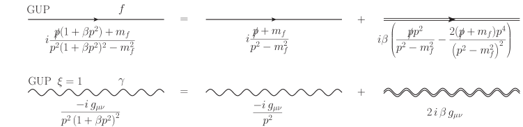
Figure 1: Modified Feynman rules for the propagators expressed as a sum of the SM contributions and the $\mathcal{O}(\beta)$ corrections.

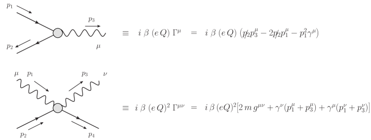
Figure 2: Feynman rules of the new QED vertices at $\mathcal{O}(\beta)$ where the momentum flow is given by the corresponding arrows. Momentum conservation reads $p_{1}=p_{2}+p_{3}$ for the 3-point vertex and, $p_{1}+p_{2}=p_{3}+p_{4}$ for the 4-point vertex.

4 Compton scattering phenomenology

The full set of diagrams that contribute to the Compton Scattering cross section at $\mathcal{O}(\beta)$ is shown in Figure 3. In the massless electron limit, the expression of the Compton cross section simply reads

$$\frac{d\sigma_{e\gamma\to e\gamma}}{d\Omega} =\frac{e^{4}\,Q^{4}}{64\,\pi^{2}s(1+\cos\theta)}\,\Big{(}2\cos\theta+\cos^{2}\theta+5+4\beta s(\cos^{2}\theta-1)\Big{)}$$

$$=\frac{d\sigma_{e\gamma\to e\gamma}^{\text{SM}}}{d\Omega}+\alpha^{2}\beta\,Q^{4}(\cos\theta-1)\,,$$ (34)

where $Q_{e}=-1$ is the charge of the electron and $e$ is the QED coupling constant. The full expression of the differential cross section including mass terms, is given in Appendix B.

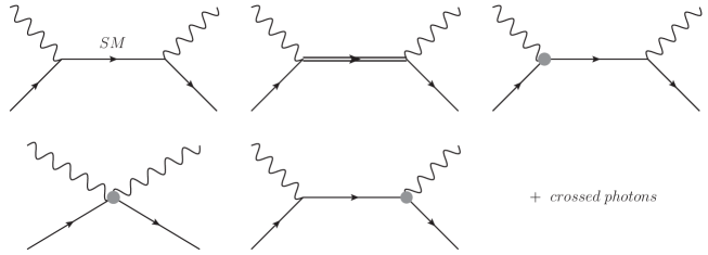
Figure 3: Feynman diagrams that contribute to Compton scattering process at $\mathcal{O}(\beta)$.

The previous expression is valid in the high-energy limit, $s\gg m^{2}$, and is therefore suitable for the phenomenological analysis presented below, where we make use of experimental data from LEP Achard_2005 . It is worth noting that, unlike the (SM) contribution, which scales as $1/s$, the GUP contribution remains constant. This feature makes high-energy experiments particularly promising for probing such new effects, as the SM background becomes increasingly suppressed while the GUP signal persists.

For the phenomenological analysis we define the $\chi^{2}$ estimator as usual,

$$\chi^{2}(\beta)=\sum_{s_{j}}\frac{\Big{(}\sigma_{e\gamma\to e\gamma}(s_{j},\beta)-\sigma_{e\gamma\to e\gamma}^{\text{exp}}(s_{j})\Big{)}^{2}}{\mu^{2}_{\text{exp}}(s_{j})}\,,$$ (35)

where $s_{j}$ are the different values of $s$ employed in the experimental analysis, $\sigma_{e\gamma\to e\gamma}(s_{j},\beta)$ is the theoretical expression for the cross section (4) integrated in between $\cos\theta=-0.8$ and $\cos\theta=0.8$, $\sigma_{e\gamma\to e\gamma}^{\text{exp}}(s_{j})$ is the experimental cross section integrated in between the same values of $\cos\theta$ and finally, $\mu^{2}_{\text{exp}}(s_{j})$ is the experimental error (standard deviation).

The results are shown in Figure 4 where we plot the $\chi^{2}$ as a function of $\beta$ (TeV^-2). Depending on the sign of the of $\beta_{0}$, at the $2\sigma$ level we find the following lower bounds

$$|\beta|^{-1/2}=|\beta_{0}|^{-1/2}\Lambda>0.68\,\text{TeV}\quad\text{with}\,\beta<0,$$ (36)

$$|\beta|^{-1/2}=|\beta_{0}|^{-1/2}\Lambda>0.25\,\text{TeV}\quad\text{with}\,\beta>0,$$ (37)

It is worth noting that the energy bounds on $|\beta_{0}|^{-1/2}\Lambda$ lie below the TeV scale, which makes it particularly appealing to further explore LHC phenomenology within the GUP framework, including potential effects on Higgs-related observables.

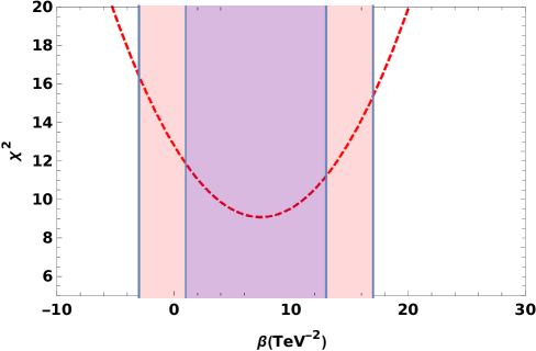
Figure 4: $\chi^{2}$ as function of $\beta$ and the corresponding $1\sigma$ and $2\sigma$ bandwidths.

Once the $\chi^{2}$ test has been performed, it is insightful to examine how our model deviates from the SM as a function of the center-of-mass energy ($s$). To carry out this analysis, we integrate over $\cos\theta$ within the angular limits previously defined, and we use the following expression:

$$\Delta\sigma=\frac{\sigma^{\text{SM}}-\sigma^{\text{GUP}}}{\sigma^{\text{SM}}}$$ (38)

The results for the upper and lower bounds of the parameter $\beta$ are shown in Figure 5.

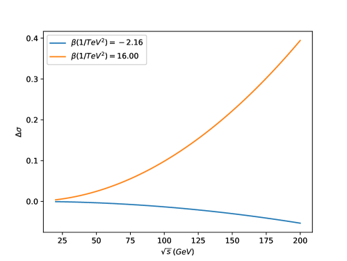
Figure 5: $\Delta\sigma$ ($\text{GeV}^{-1}$) as function of $\sqrt{s}$ for two values of $\beta$ that correspond to the lower bounds (37).

From the initial analysis, we observe that the positive bound leads to larger deviations from the SM and becomes relevant at lower energies than the negative bound. Specifically, for the observable associated with the Compton scattering process, the contribution from the Generalized Uncertainty Principle at leading order $\mathcal{O}(\beta)$ reaches approximately $40\%$ near an energy scale of 200 GeV.

It is also instructive to analyze the angular dependence of the GUP contribution at high energies. As illustrated in Figure 6, the largest discrepancies between the SM and GUP predictions occur at incidence angles close to $\pi/2$ (low values of $\cos\theta$). For the negative $2\sigma$ bound, the GUP contribution differs from the SM prediction by around $10\%$, whereas for the positive $2\sigma$ bound, the deviation increases to nearly $50\%$. These results suggest that, at an energy scale of 200 GeV, the effects introduced by the modified commutation relations may be experimentally observable in the angular distribution of the cross section.

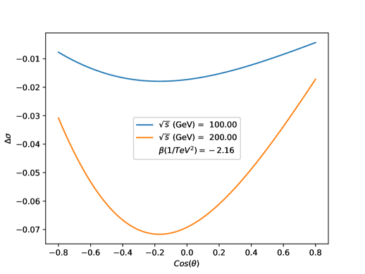
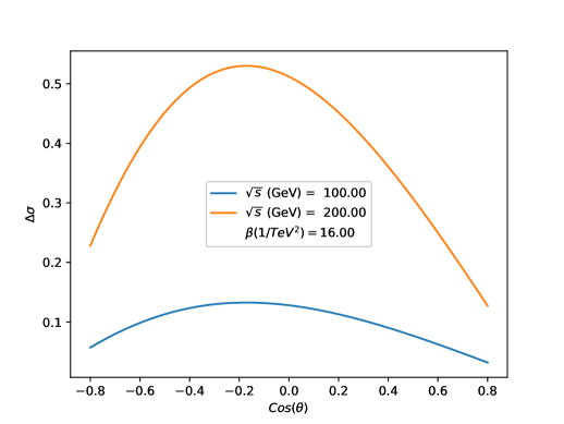
Figure 6: The deviation between the Standard Model and the GUP prediction $\Delta\sigma$ as a function of $\cos\theta$ for $\sqrt{s}=100$ (blue) and $200$ GeV (orange) for the two lower bounds on $\beta$ obtained in (37).

5 Conclusions

In this work, we have presented a consistent formulation of Quantum Electrodynamics within the framework of the Generalized Uncertainty Principle, incorporating the effects of a modified set of commutation relations, encoded in a free parameter $\beta$. Starting from first principles, we have shown that maintaining both gauge and Lorentz invariance requires the inclusion of an additional $k$-space where the commutation relations hold as usual. This leads to a modified, consistent, effective field theory with new vertices and propagators contributing at $\mathcal{O}(\beta)$.

Using this effective GUP-QED Lagrangian, we performed a detailed phenomenological analysis of the Compton scattering process. Our results show that the GUP contributions lead to measurable deviations from the Standard Model predictions, with discrepancies of up to $40\%$ at energies around 200 GeV for the positive $2\sigma$ bound. Angular analyses further reveal that such deviations can reach $50\%$ at low incidence angles, highlighting the potential for experimental detection.

Importantly, the derived bounds on $\beta$ lie below the TeV scale, making future studies at the LHC, especially those involving Higgs-related observables, particularly promising in the search for GUP effects that could ultimately be related to effective, or even fundamental, quantum gravity theories. Our results demonstrate that effective field theory techniques can be successfully employed to bridge quantum gravity scenarios with high-energy phenomenology, offering a testable path for exploring minimal length effects in current and upcoming collider experiments.

The results obtained in this study motivate further investigation of GUP effects in high-energy processes at current and future colliders. In particular, while our analysis has focused on energy scales up to a few hundred GeV, the LHC and proposed future facilities such as the Future Circular Collider (FCC) offer access to significantly higher energies and improved experimental precision. However, the FCC-ee phase Suarez:2022pcn ; Blondel:2019jmp is expected to operate at center-of-mass energies ranging from 90 to 365 GeV, which aligns remarkably well with the energy range explored in Figures 5 and 6, making our results directly relevant for future precision tests at the FCC.

The FCC, with a projected center-of-mass energy of up to 100 TeV and expected integrated luminosities surpassing those of the HL-LHC, is anticipated to achieve percent-level precision in key electroweak and QED observables. This level of sensitivity opens the possibility of probing GUP-induced deviations well beyond current limits. Higgs physics, diboson production, and precision QED processes at the FCC-ee phase, in particular, could serve as clean environments to test the presence of GUP-induced effects, especially in angular distributions and differential cross sections.

Future work will focus on extending the effective GUP-QED framework to other processes of phenomenological interest such as Higgs decays, electron and muon $(g-2)$ or loop-level corrections. Furthermore, incorporating renormalization group effects and developing a systematic approach to higher-order $\beta$ corrections could refine the predictions and improve the robustness of the bounds.

Appendix A Calculation of the Modified Feynman Propagators

The Feynman propagator $\Delta_{F}(x)$ for the modified Klein-Gordon field must satisfy

$$\Big{(}\square(1-\beta\square)^{2}+m^{2}\Big{)}\Delta_{F}(x)=-\delta^{(4)}(x)\,.$$ (39)

The solution can be found straightforwardly i.e., it is simply given by

$$\Delta_{F}(x)=\int\frac{d^{4}p}{(2\pi)^{4}}\frac{e^{-ipx}}{p^{2}(1+\beta p^{2})^{2}-m^{2}+i\epsilon}\,,$$ (40)

and so, the Klein-Gordon field propagator will be given, in momentum space, by

$$\frac{i}{p^{2}(1+\beta p^{2})^{2}-m^{2}}=\frac{i}{p^{2}-m^{2}}+\beta\frac{-2\,i\,p^{4}}{(p^{2}-m^{2})^{2}}+\mathcal{O}(\beta^{2})\,.$$ (41)

In the previous equation we have ignored the $i\epsilon$ term, and we shall also do so in the following. The fermionic Feynman propagator $S_{F}(x)$ must satisfy the modified equation

$$S_{F}(x)=\Big{(}i\not{\partial}(1-\beta\square)+m\Big{)}\Delta_{F}(x)\,,$$ (42)

and so, we can easily find the expression for the propagator to be

$$\frac{i\big{(}\not{p}(1+\beta p^{2})+m\big{)}}{p^{2}(1+\beta p^{2})^{2}-m^{2}}=\frac{i(\not{p}+m)}{p^{2}-m^{2}}+i\,\beta\left(\frac{\not{p}\,p^{2}}{p^{2}-m^{2}}-\frac{2p^{4}(\not{p}+m)}{(p^{2}-m^{2})^{2}}\right)+\mathcal{O}(\beta^{2})\,.$$ (43)

In order to find the Feynman propagator of the photon field, let us take a closer look at the photon kinetic terms from (3). If we chose a an appropriate gauge fixing term, i.e.,

$$\mathcal{L}^{\text{GUP}}_{A,\xi}=-\frac{1}{4}F^{\mu\nu}F_{\mu\nu}+\frac{\beta}{2}F^{\mu\nu}\Big{(}\square F_{\mu\nu}\Big{)}-\frac{1}{2\xi}\Big{(}\partial_{\mu}(1-\beta\square)A^{\mu}\Big{)}^{2}\,,$$ (44)

we obtain the following equation of motion for the photon field

$$\left(g^{\mu\nu}\square(1-\beta\square)^{2}+\left(\frac{1}{\xi}-1\right)\partial^{\mu}\partial^{\nu}(1-\beta\square)^{2}\right)A_{\nu}\equiv O^{\mu\nu}_{\xi}A_{\nu}=0\,.$$ (45)

The Feynman propagator must then satisfy

$$O^{\mu\nu}_{\xi}\,D^{F}_{\nu\alpha}(x)=\delta^{\mu}_{\alpha}\delta^{(4)}(x)\,.$$ (46)

Choosing the Feynman gauge $\xi=1$ we can straightforwardly obtain

$$D^{F}_{\mu\nu}=\int\frac{d^{4}p}{(2\pi)^{4}}\frac{-g_{\mu\nu}\,e^{-ipx}}{p^{2}(1+\beta p^{2})^{2}+i\epsilon}\,,$$ (47)

which gives rise to the simple Feynman rule

$$\frac{-i\,g_{\mu\nu}}{p^{2}(1+\beta p^{2})^{2}}=-i\,\frac{g_{\mu\nu}}{p^{2}}+2\,i\,\beta\,g_{\mu\nu}\,.$$ (48)

Let us finally turn our attention to the massive gauge fields $V$ (with $V=W,Z$). The corresponding GUP-modified equation, in the unitary gauge, will be given by

$$\left(g^{\mu\nu}\left(\square(1-\beta\square)^{2}+m^{2}\right)-\partial^{\mu}\partial^{\nu}(1-\beta\square)^{2}\right)V_{\nu}\equiv O_{V}^{\mu\nu}V_{\nu}=0\,,$$ (49)

and so, the equation that the propagator of the gauge fields $V$ must satisfy is

$$O_{V}^{\mu\nu}D_{\mu\alpha}^{F,V}(x)=\delta_{\alpha}^{\mu}\delta^{(4)}(x)\,,$$ (50)

and so, the propagator, in the unitary gauge and in momentum space, up to $\mathcal{O}(\beta)$, is simply given by the following expression

$$\frac{1}{p^{2}-m^{2}}\left(-g_{\mu\nu}+\frac{p_{\mu}p_{\nu}}{m^{2}}\right)+\frac{2\beta\,p^{4}}{\left(p^{2}-m^{2}\right)^{2}}\left(g_{\mu\nu}-\frac{p_{\mu}p_{\nu}}{p^{2}}\right)+\mathcal{O}\left(\beta^{2}\right)\,.$$ (51)

Appendix B Full Expression of the Compton Cross Section

The unpolarized, spin averaged, squared amplitude at $\mathcal{O}(\beta)$ for the process is given by the sum

$$|\overline{\mathcal{M}}|^{2}=\frac{1}{4}\left(\,|{\mathcal{M}}_{\text{SM}}|^{2}+2\,\text{Re}[\mathcal{M}_{\text{SM}}^{\dagger}\,\mathcal{M}_{\text{GUP}}]\,\right),$$ (52)

with the following expressions for the two contributions

$$|\mathcal{M}_{\text{SM}}|^{2} =\frac{8e^{4}Q^{4}}{\left(m^{2}-{s}\right)^{2}\left(m^{2}-{u}\right)^{2}}\Big{(}6m^{8}-m^{4}\left(3{s}^{2}+14{s}{u}+3\text{u}^{2}\right)$$

$$\qquad\qquad\qquad\qquad+m^{2}({s}+{u})\left({s}^{2}+6{s}{u}+{u}^{2}\right)-{s}{u}\left({s}^{2}+{u}^{2}\right)\Big{)}$$ (53)

and,

$$2\,\text{Re}[\mathcal{M}_{\text{SM}}^{\dagger}\,\mathcal{M}_{\text{GUP}}] =\frac{16\beta e^{4}Q^{4}}{\left(m^{2}-{s}\right)^{3}\left(m^{2}-{u}\right)^{3}}\Big{(}-2{s}^{3}{u}^{3}({s}+{u})+22m^{14}-2m^{12}(7{s}+9{u})$$

$$\qquad+m^{10}\left(-5{s}^{2}-46{s}{u}+5{u}^{2}\right)+m^{8}\left(7{s}^{3}+51{s}^{2}{u}+35{s}{u}^{2}-{u}^{3}\right)$$

$$\qquad-2m^{6}{s}\left({s}^{3}+6{s}^{2}{u}-2{s}{u}^{2}-2{u}^{3}\right)+m^{4}{s}{u}\left({s}^{3}-23{s}^{2}{u}-31{s}{u}^{2}-3{u}^{3}\right)$$

$$\qquad+m^{2}{s}^{2}{u}^{2}\left(3{s}^{2}+22{s}{u}+5{u}^{2}\right)\Big{)}\,.$$ (54)

The expression of the total differential cross-section in the center of mass is given by

$$\frac{d\sigma_{e\gamma\to e\gamma}}{d\Omega} =\frac{1}{64\pi^{2}s^{2}u}|\overline{\mathcal{M}}|^{2}\,,$$ (55)

where $u$ can be expressed as a function of $\cos\theta$ as usually

$$u=m^{2}-\frac{s}{2}-\frac{(s-m^{2})^{2}}{2s}\,\cos\theta\,.$$ (56)

References

- (1) M. Maggiore, The Algebraic structure of the generalized uncertainty principle, Phys. Lett. B 319 (1993) 83–86, [hep-th/9309034].
- (2) A. Kempf, G. Mangano, and R. B. Mann, Hilbert space representation of the minimal length uncertainty relation, Physical Review D 52 (July, 1995) 1108–1118.
- (3) F. Scardigli, Generalized uncertainty principle in quantum gravity from micro-black hole gedanken experiment, Physics Letters B 452 (Apr., 1999) 39–44.
- (4) J. Y. Bang and M. S. Berger, Quantum Mechanics and the Generalized Uncertainty Principle, Phys. Rev. D 74 (2006) 125012, [gr-qc/0610056].
- (5) P. Bosso, G. G. Luciano, L. Petruzziello, and F. Wagner, 30 years in: Quo vadis generalized uncertainty principle?, Class. Quant. Grav. 40 (2023), no. 19 195014, [arXiv:2305.1619].
- (6) P. Pedram, New Approach to Nonperturbative Quantum Mechanics with Minimal Length Uncertainty, Phys. Rev. D 85 (2012) 024016, [arXiv:1112.2327].
- (7) P. Galan and G. A. Mena Marugan, Canonical Realizations of Doubly Special Relativity, Int. J. Mod. Phys. D 16 (2007) 1133–1147, [gr-qc/0702027].
- (8) S. Das and S. Pramanik, Path Integral for non-relativistic Generalized Uncertainty Principle corrected Hamiltonian, Phys. Rev. D 86 (2012) 085004, [arXiv:1205.3919].
- (9) P. Pedram, A Higher Order GUP with Minimal Length Uncertainty and Maximal Momentum, Phys. Lett. B 714 (2012) 317–323, [arXiv:1110.2999].
- (10) S. Mignemi, Classical and quantum mechanics of the nonrelativistic Snyder model in curved space, Class. Quant. Grav. 29 (2012) 215019, [arXiv:1110.0201].
- (11) K. Nozari and A. Etemadi, Minimal length, maximal momentum and Hilbert space representation of quantum mechanics, Phys. Rev. D 85 (2012) 104029, [arXiv:1205.0158].
- (12) L. Tedesco, Fine Structure Constant, Domain Walls, and Generalized Uncertainty Principle in the Universe, Int. J. Math. Math. Sci. 2011 (2011) 543894, [arXiv:1106.3436].
- (13) V. Balasubramanian, S. Das, and E. C. Vagenas, Generalized Uncertainty Principle and Self-Adjoint Operators, Annals Phys. 360 (2015) 1–18, [arXiv:1404.3962].
- (14) V. M. Tkachuk, Galilean and Lorentz Transformations in a Space with Generalized Uncertainty Principle, Found. Phys. 46 (2016), no. 12 1666–1679, [arXiv:1310.6243].
- (15) P. Bosso, L. Petruzziello, and F. Wagner, The minimal length is physical, Phys. Lett. B 834 (2022) 137415, [arXiv:2206.0506].
- (16) S. Pramanik and S. Ghosh, GUP-based and Snyder Non-Commutative Algebras, Relativistic Particle models and Deformed Symmetries and Interaction: A Unified Approach, Int. J. Mod. Phys. A 28 (2013), no. 27 1350131, [arXiv:1301.4042].
- (17) P. Bosso, Rigorous Hamiltonian and Lagrangian analysis of classical and quantum theories with minimal length, Phys. Rev. D 97 (2018), no. 12 126010, [arXiv:1804.0820].
- (18) W. S. Chung and H. Hassanabadi, New generalized uncertainty principle from the doubly special relativity, Phys. Lett. B 785 (2018) 127–131, [arXiv:1807.1155].
- (19) P. Bosso, S. Das, and V. Todorinov, Quantum field theory with the generalized uncertainty principle I: Scalar electrodynamics, Annals Phys. 422 (2020) 168319, [arXiv:2005.0377].
- (20) P. Bosso, S. Das, and V. Todorinov, Quantum field theory with the generalized uncertainty principle II: Quantum Electrodynamics, Annals Phys. 424 (2021) 168350, [arXiv:2005.0377].
- (21) S. Hossenfelder, Interpretation of quantum field theories with a minimal length scale, Physical Review D 73 (May, 2006).
- (22) S. Das, M. P. Robbins, and M. A. Walton, Generalized uncertainty principle corrections to the simple harmonic oscillator in phase space, Canadian Journal of Physics 94 (Jan., 2016) 139–146.
- (23) L. Maccone and A. K. Pati, Stronger uncertainty relations for all incompatible observables, Physical Review Letters 113 (Dec., 2014).
- (24) A. Tawfik and A. Diab, Generalized uncertainty principle: Approaches and applications, International Journal of Modern Physics D 23 (Oct., 2014) 1430025.
- (25) S. Hossenfelder, Minimal length scale scenarios for quantum gravity, Living Reviews in Relativity 16 (Jan., 2013).
- (26) V. Nenmeli, S. Shankaranarayanan, V. Todorinov, and S. Das, Maximal momentum gup leads to quadratic gravity, Physics Letters B 821 (Oct., 2021) 136621.
- (27) D. Chen, H. Wu, and H. Yang, Fermion’s tunnelling with effects of quantum gravity, Advances in High Energy Physics 2013 (2013) 1–6.
- (28) S. Basilakos, S. Das, and E. C. Vagenas, Quantum gravity corrections and entropy at the planck time, Journal of Cosmology and Astroparticle Physics 2010 (Sept., 2010) 027–027.
- (29) G. Gecim and Y. Sucu, The gup effect on hawking radiation of the 2 + 1 dimensional black hole, Physics Letters B 773 (Oct., 2017) 391–394.
- (30) G. Gecim and Y. Sucu, Quantum gravity effect on the tunneling particles from 2 + 1-dimensional new-type black hole, Advances in High Energy Physics 2018 (2018) 1–7.
- (31) K. Konishi, G. Paffuti, and P. Provero, Minimum physical length and the generalized uncertainty principle in string theory, Physics Letters B 234 (1990), no. 3 276–284.
- (32) L. N. Chang, Z. Lewis, D. Minic, and T. Takeuchi, On the minimal length uncertainty relation and the foundations of string theory, Advances in High Energy Physics 2011 (2011) 1–30.
- (33) A. H. Gomes, Constraining gup models using limits on sme coefficients, Classical and Quantum Gravity 39 (Oct., 2022) 225017.
- (34) S. Das and E. C. Vagenas, Universality of quantum gravity corrections, Physical Review Letters 101 (Nov., 2008).
- (35) A. F. Ali, M. M. Khalil, and E. C. Vagenas, Minimal length in quantum gravity and gravitational measurements, 2015.
- (36) M. F. e. a. Marin, Francesco, Gravitational bar detectors set limits to planck-scale physics on macroscopic variables, Nature Physics 9 (Oct., 2013) 225017.
- (37) S. Hossenfelder, Minimal Length Scale Scenarios for Quantum Gravity, Living Rev. Rel. 16 (2013) 2, [arXiv:1203.6191].
- (38) P. Achard, Compton scattering of quasi-real virtual photons at lep, Physics Letters B 616 (June, 2005) 145–158.
- (39) S. Hossenfelder, Running coupling with minimal length, Phys. Rev. D 70 (2004) 105003, [hep-ph/0405127].
- (40) C. Quesne and V. M. Tkachuk, Lorentz-covariant deformed algebra with minimal length, Czech. J. Phys. 56 (2006) 1269–1274, [quant-ph/0612093].
- (41) M. Kober, Gauge Theories under Incorporation of a Generalized Uncertainty Principle, Phys. Rev. D 82 (2010) 085017, [arXiv:1008.0154].
- (42) M. Kober, Electroweak Theory with a Minimal Length, Int. J. Mod. Phys. A 26 (2011) 4251–4285, [arXiv:1104.2319].
- (43) V. Husain, D. Kothawala, and S. S. Seahra, Generalized uncertainty principles and quantum field theory, Phys. Rev. D 87 (2013), no. 2 025014, [arXiv:1208.5761].
- (44) M. Faizal and T. S. Tsun, Topological defects in a deformed gauge theory, Nucl. Phys. B 924 (2017) 588–602, [arXiv:1711.0749].
- (45) V. Todorinov, P. Bosso, and S. Das, Relativistic Generalized Uncertainty Principle, Annals Phys. 405 (2019) 92–100, [arXiv:1810.1176].
- (46) S. Hossenfelder, The Soccer-Ball Problem, SIGMA 10 (2014) 074, [arXiv:1403.2080].
- (47) R. G. Suarez, The Future Circular Collider (FCC) at CERN, PoS DISCRETE2020-2021 (2022) 009, [arXiv:2204.1002].
- (48) A. Blondel et al., Polarization and Centre-of-mass Energy Calibration at FCC-ee, arXiv:1909.1224.