An Extension of the Adiabatic Theorem

Abstract

We examine the validity of a potential extension of the adiabatic theorem to quantum quenches, i.e., non-adiabatic changes. In particular, the Transverse Field Ising Model (TFIM) and the Axial Next Nearest Neighbour Ising (ANNNI) model are studied. The proposed extension of the adiabatic theorem is stated as follows: Consider the overlap between the initial ground state and the post-quench Hamiltonian eigenstates for quenches within the same phase. This overlap is largest for the post-quench ground state. In the case of the TFIM, this conjecture is confirmed for both the paramagnetic and ferromagnetic phases numerically and analytically. In the ANNNI model, the conjecture could be analytically proven for a special case. Numerical methods were employed to investigate the conjecture’s validity beyond this special case.

I Introduction

Understanding the connection between ground states and eigenstates after a quantum quench can advance our understanding of non-equilibrium dynamics in quantum systems. Specifically, studying how ground states behave after quenches sheds light on energy distributions and phase transition dynamics. Hence, predicting overlaps between eigenstates can provide important insights into the mechanisms governing quench dynamics in non-equilibrium many-body systems.

Quantum quenches and adiabatic time evolution represent two extremes in the study of quantum dynamics, both of which have been the subject of extensive theoretical and numerical research. Previous experimental [1, 2, 3, 4] and theoretical [5, 6, 3] works have explored the evolution of ground states in quenched systems and how memory of the system’s initial state is retained. Quench dynamics have been used to study and identify phase transitions, either directly [7, 8] or through out-of-time-order correlators (OTOCs) [9]. This work investigates the extent to which statements about ground state overlaps hold in the context of quantum quenches. In that sense, it seeks to extend the adiabatic theorem to maximally non-adiabatic changes.

After presenting the conjecture and its connection to the adiabatic theorem in section II we present analytical results for two specific models, the Transverse Field Ising Model (TFIM) and the Axial Next Nearest Neighbour Ising (ANNNI) model. For the TFIM we conduct a full analytical proof in section III, whereas for the ANNNI model only a special case is proven analytically in section IV. To investigate the conjecture’s validity beyond this special case, section V contains a numerical analysis. In section VII we summarise our results and give an outlook to future investigations.

II Conjecture

The adiabatic theorem, formulated by Max Born and Vladimir Fock in 1928, states [10]:

A physical system remains in its instantaneous eigenstate if a given perturbation is acting on it slowly enough and if there is a gap between the eigenvalue and the rest of the Hamiltonian’s spectrum.

This statement can be re-expressed in terms of quantum state overlaps: consider a quantum system with an initial Hamiltonian $\mathcal{H}_{i}$ at time $t<0$, whose eigenstates are denoted by $|\psi_{n}\rangle$. Without loss of generality, assume the system to be in its ground state, with an excitation gap $\Delta$ above it. At $t=0$, a perturbation acts on the system, such that the eigenstates evolve under the time-dependent Schrödinger equation to $|\psi_{n}(t>0)\rangle$. Let $\mathcal{H}_{f}$ denote the perturbed Hamiltonian, which typically has a different set of eigenstates $|\widetilde{\psi_{n}}\rangle$. For a perturbation with arbitrarily large ramping time $\tau$, the overlap of the time-evolved initial ground state and the final ground state is approaching 1 arbitrarily closely:

$$\lim_{\tau\rightarrow\infty}|\langle\text{GS}(t>0)\mid\widetilde{\text{GS}}\rangle|^{2}=1.$$ (1)

Any time-evolution of a quantum system is called “adiabatic” if it happens slowly enough. That is the case if the evolution is much slower than the inverse energy gap size, $\tau\gg\Delta^{-1}$.

The primary objective of this work is to investigate the relationship between eigenstates of different Hamiltonians when the system is quenched, i.e., when the adiabatic assumption is no longer valid. Explicitly, this paper aims to test the validity of a conjecture, which can be formulated as follows:

The overlap of the initial ground state $|\text{GS}\rangle$ with any post-quench eigenstate $|\widetilde{\psi_{n}}\rangle$ is maximal if $|\widetilde{\psi_{n}}\rangle$ is the post-quench ground state, as long as both Hamiltonians are in the same phase:

$$\operatorname{max}_{n}|\langle\text{GS}\mid\widetilde{\psi_{n}}\rangle|^{2}=|\langle\text{GS}\mid\widetilde{\text{GS}}\rangle|^{2}.$$ (2)

As a necessary condition, we restrict the validity of the conjecture to systems with a continuous spectrum. Since the concept of phase transitions is only well-defined in the thermodynamic limit, the conjecture is expected to hold asymptotically for finite systems.

III Transverse Field Ising Model

The Hamiltonian of the one-dimensional TFIM is given by

$$H_{\text{TFIM}}=-J\sum_{j}\left(\sigma_{j}^{z}\sigma_{j+1}^{z}+h\sigma_{j}^{x}\right),$$ (3)

where $\sigma^{x}$ and $\sigma^{z}$ denote Pauli matrices. The parameter $J$ denotes an overall energy scale, subsequently set equal to one for convenience, while $h>0$ defines the strength of the transverse magnetic field. At zero temperature, this model undergoes a phase transition from a gapped ferromagnet to a gapped paramagnet at a critical value of $h=J$ [11].

After Jordan-Wigner [12] and Bogoliubov [13] transformations, the Hamiltonian reads

$$H_{\text{TFIM}}=\sum_{k>0}\bigg{(}\epsilon_{k}\bigg{(}\gamma_{k}^{\dagger}\gamma_{k}-\gamma_{-k}\gamma_{-k}^{\dagger}\bigg{)}-h\bigg{)}.$$ (4)

This is the starting point for the subsequent calculations, where the general idea is to quench from an initial (pre-quench) Hamiltonian $H_{i}$ to a final (post-quench) Hamiltonian $H_{f}$:

$$H_{i}\ \xrightarrow{t\ll\Delta^{-1}}\ H_{f}.$$ (5)

In general, these Hamiltonians $H_{i}$ and $H_{f}$ have different eigenbases and the pre-quench ground state expressed in the post-quench eigenbasis takes the form

$$|\text{GS}(h)\rangle=\frac{1}{\mathcal{N}}\exp{\bigg{(}\sum_{k>0}B^{*}(k)\gamma_{k}^{\dagger}\gamma_{-k}^{\dagger}\bigg{)}}|0,0\rangle.$$ (6)

This Eq. (6) is valid for any value of $h$, and therefore applies in both the paramagnetic and the ferromagnetic phase.

The coefficient $B(k)$ is defined by [11]

$$B(k):=-i\frac{V_{k}}{U_{k}}=-i\ \tan(\theta_{k}(h_{i})-\theta_{k}(h_{f})),$$ (7)

where the coefficients $V_{k}$ and $U_{k}$ are given by

$$\begin{split}U_{k}&=\cos(\theta_{k}(h_{i}))\cos(\theta_{k}(h_{f}))+\sin(\theta_{k}(h_{i}))\sin(\theta_{k}(h_{f})),\\ V_{k}&=\cos(\theta_{k}(h_{i}))\sin(\theta_{k}(h_{f}))-\sin(\theta_{k}(h_{i}))\cos(\theta_{k}(h_{f})).\end{split}$$ (8)

For the excited states of the post-quench Hamiltonian in its own eigenbasis, there are three different possibilities:

$$|0,1\rangle =\gamma_{k}^{\dagger}|0,0\rangle,$$ (9)

$$|1,0\rangle =\gamma_{-k}^{\dagger}|0,0\rangle,\text{ and}$$ (10)

$$|1,1\rangle =\gamma_{k}^{\dagger}\gamma_{-k}^{\dagger}|0,0\rangle.$$ (11)

The excitations in Eq.s (9) and (10) involve unpaired creation operators, resulting in zero overlap with the pre-quench ground state. The more interesting excitations are those in Eq. (11), as they involve paired creation operators and can have non-zero overlaps with the pre-quench ground state.

We first calculate the ground state overlap:

$$\begin{split}|\langle\text{GS}(h)\mid 0,0\rangle|^{2}&=\bigg{|}\frac{1}{\mathcal{N}}\langle 0,0\mid\exp{\bigg{(}\sum_{k>0}B(k)\gamma_{-k}\gamma_{k}\bigg{)}}\mid 0,0\rangle\bigg{|}^{2}\\ &=\frac{1}{\mathcal{N}^{2}}\bigg{|}\langle 0,0\mid\prod_{k>0}\bigg{(}1+B(k)\gamma_{-k}\gamma_{k}\bigg{)}\mid 0,0\rangle\bigg{|}^{2}\\ &=\frac{1}{\mathcal{N}^{2}}.\end{split}$$ (12)

Then, we compute the overlap of the pre-quench ground state with the post-quench excited state as defined in Eq. (11):

$$\begin{split}|\langle\text{GS}(h)\mid 1,1\rangle|^{2}&=\frac{1}{\mathcal{N}^{2}}\bigg{|}\langle 0,0\mid\exp{\bigg{(}\sum_{k>0}B(k)\gamma_{-k}\gamma_{k}\bigg{)}}\gamma_{-k^{\prime}}^{\dagger}\gamma_{k^{\prime}}^{\dagger}\mid 0,0\rangle\bigg{|}^{2}\\ &=\frac{1}{\mathcal{N}^{2}}\bigg{|}B(k^{\prime})\bigg{|}^{2}.\end{split}$$ (13)

Inserting the definition (7) for $B(k)$ into this expression yields

$$\bigg{|}\langle\text{GS}(h)\mid 1,1\rangle\bigg{|}^{2}=\frac{1}{\mathcal{N}^{2}}\tan^{2}\bigg{(}\theta_{k}(h_{i})-\theta_{k}(h_{f})\bigg{)}.$$ (14)

Expression (14) must be smaller than the ground state overlap (12) for the conjecture to be correct, hence

$$\bigg{|}\langle\text{GS}(h)\mid 1,1\rangle\bigg{|}^{2}\overset{!}{<}\bigg{|}\langle\text{GS}(h)\mid 0,0\rangle\bigg{|}^{2}$$ (15)

$$\Leftrightarrow\ \ \frac{1}{\mathcal{N}^{2}}\tan^{2}\bigg{(}\theta_{k}(h_{i})-\theta_{k}(h_{f})\bigg{)}\overset{!}{<}\frac{1}{\mathcal{N}^{2}}$$ (16)

$$\Leftrightarrow\ \ \tan^{2}\bigg{(}\theta_{k}(h_{i})-\theta_{k}(h_{f})\bigg{)}\overset{!}{<}1.$$ (17)

This condition (17) is fulfilled if and only if the argument of $\tan^{2}(x)$ lies in the interval $[-\frac{\pi}{4},\frac{\pi}{4}]$. We conclude

$$\bigg{|}\theta_{k}(h_{i})-\theta_{k}(h_{f})\bigg{|}\overset{!}{<}\frac{\pi}{4}.$$ (18)

The angles $\theta_{k}(h)$ are known to lie in $[0,\frac{\pi}{2}]$ with their explicit expressions given by the parameterisation of the Bogoliubov transformation [11]

$$\tan(2\theta_{k})=\frac{\sin k}{h-\cos k}\ \Leftrightarrow\ \theta_{k}(h)=\frac{1}{2}\arctan\bigg{(}\frac{\sin k}{h-\cos k}\bigg{)}.$$ (19)

As $k=2\pi\frac{n}{L}$, with $n\in\mathbb{N}$ in the interval $[1,\frac{L}{2}]$ and $L$ being the spin chain length, the values for $k$ cover half a period from 0 to $\pi$. Using the inverse tangent function

$$\tan^{-1}(2\theta_{k})=\begin{cases}\arctan(2\theta_{k}),\quad 2\theta_{k}>0\\ \arctan(2\theta_{k})+\pi,\quad 2\theta_{k}<0,\end{cases}$$ (20)

implies for the definition of $\theta_{k}(h)$

$$\theta_{k}(h)=\begin{cases}\frac{1}{2}\arctan\bigg{(}\frac{\sin k}{h-\cos k}\bigg{)},\quad\frac{\sin k}{h-\cos k}>0\\ \frac{1}{2}\bigg{(}\arctan(\frac{\sin k}{h-\cos k})+\pi\bigg{)},\quad\frac{\sin k}{h-\cos k}<0.\end{cases}$$ (21)

The condition on the left-hand side of Eq. (17) depends on three variables, $h_{i}$, $h_{f}$, and $k$. Its maximum with respect to each of these variables is computed, leading to the distinction of three different scenarios:

1. Both Hamiltonians lie in the paramagnetic phase. Without loss of generality, it is assumed that $1<h_{i}<h_{f}$. In the paramagnetic phase, $\theta_{k}=\frac{1}{2}\arctan(\frac{\sin k}{h-\cos k})\forall h_{i},h_{f},k$ as $\frac{\sin k}{h-\cos k}>0$ for all values of $h_{i},h_{f}\in(1,\infty)$ and $k\in[0,\pi]$.
   

   The $\arctan(\frac{\sin k}{h_{i}-\cos k})$ is a monotonically decreasing function in $h$ for all $k\in[0,\pi]$. Therefore, the maximal difference of $\theta_{k}(h_{i})$ and $\theta_{k}(h_{f})$ is reached for maximally different $h_{i}$ and $h_{f}$. We choose $h_{i}$ to be $1+\epsilon$ with $\epsilon\rightarrow 0$ and $h_{f}$ to be $x\rightarrow\infty$ and obtain

   $$\max_{h_{i},h_{f},k}\bigg{(}\bigg{|}\theta_{k}(h_{i})-\theta_{k}(h_{f})\bigg{|}\bigg{)}=\frac{\pi}{4}.$$ (22)

   As the function approaches the limit from below, the conjecture (2) is fulfilled for all possible parameter combinations of $h_{i}$, $h_{f}$ and $k$ in the paramagnetic phase.

2. Both Hamiltonians lie in the ferromagnetic phase. Without loss of generality, it is assumed that $0\leq h_{i}<h_{f}<1$. For $h\in[0,1)$, we rewrite Eq. (21):

   $$\theta_{k}(h)=\begin{cases}\frac{1}{2}\arctan\bigg{(}\frac{\sin k}{h-\cos k}\bigg{)},\quad k>\arccos(h)\\ \frac{1}{2}\bigg{(}\arctan\bigg{(}\frac{\sin k}{h-\cos k}\bigg{)}+\pi\bigg{)},\quad k<\arccos(h).\end{cases}$$ (23)

   We consider $\arccos(h)<k=\arccos(h)+\nu$ with $\nu>0$.

   $$\begin{split}&\max_{h_{i},h_{f},k}\bigg{(}\bigg{|}\theta_{k}(h_{i})-\theta_{k}(h_{f})\bigg{|}\bigg{)}\\ =&\max_{h_{i},h_{f},\nu}\bigg{(}\frac{1}{2}\bigg{|}\arctan\bigg{(}\frac{\sin(\arccos(h_{i})+\nu)}{h_{i}-\cos(\arccos(h_{i})+\nu)}\bigg{)}\\ &\quad\quad\quad\ -\arctan\bigg{(}\frac{\sin(\arccos(h_{f})+\nu)}{h_{f}-\cos(\arccos(h_{f})+\nu)}\bigg{)}\bigg{|}\bigg{)}\end{split}$$ (24)

   As the $\arctan(\cdot)$ is a monotone function in $h$ for all $\nu\in(0,\pi]$, the maximal difference of $\theta_{k}(h_{i})$ and $\theta_{k}(h_{f})$ is reached for maximally different $h_{i}$ and $h_{f}$. Thus, we choose $h_{i}$ to be $0$ and $h_{f}$ to be $1-\epsilon$ with $\epsilon\rightarrow 0$, such that

   $$=\max_{\nu}\bigg{(} \frac{1}{2}\bigg{|}\arctan\bigg{(}\frac{\sin(\frac{\pi}{2}+\nu)}{\cos(\frac{\pi}{2}+\nu)}\bigg{)}$$ (25)

   $$+\arctan\bigg{(}\frac{\sin(\nu)}{1-\cos(\nu)}\bigg{)}\bigg{|}\bigg{)}$$ (26)

   follows. For $k\in[0,\pi]$ to be fulfilled, it becomes apparent that $\nu\overset{!}{\in}(0,\frac{\pi}{2}]$ and

   $$\max_{h_{i},h_{f},k}\bigg{(}\bigg{|}\theta_{k}(h_{i})-\theta_{k}(h_{f})\bigg{|}\bigg{)}=\frac{\pi}{8}<\frac{\pi}{4}.$$ (27)

   Hence, the conjecture (2) is confirmed for this choice of $\theta_{k}(h)$.

3. Again, both Hamiltonians lie in the ferromagnetic phase. As before, without loss of generality, it is assumed that $0<h_{i}<h_{f}<1$. However, now we consider the case of $\arccos(h)>k=\arccos(h)-\nu$ with $\nu>0$. From $k\in[0,\pi]$ it follows that $\nu\overset{!}{\in}[-\frac{\pi}{2},0)$.

   $$\begin{split}&\max_{h_{i},h_{f},k}\bigg{(}\bigg{|}\theta_{k}(h_{i})-\theta_{k}(h_{f})\bigg{|}\bigg{)}\\ =&\max_{h_{i},h_{f},\nu}\bigg{(}\frac{1}{2}\bigg{|}\arctan\bigg{(}\frac{\sin(\arccos(h_{i})-\nu)}{h_{i}-\cos(\arccos(h_{i})-\nu)}\bigg{)}+\pi\\ &\quad\quad\quad\quad-\arctan\bigg{(}\frac{\sin(\arccos(h_{f})-\nu)}{h_{f}-\cos(\arccos(h_{f})-\nu)}\bigg{)}+\pi\bigg{|}\bigg{)}\end{split}$$ (28)

   As $\arctan(\cdot)$ is a monotone function in $h$ for all $\nu\in[-\frac{\pi}{2},0)$, the maximal difference of $\theta_{k}(h_{i})$ and $\theta_{k}(h_{f})$ is again reached for maximally different $h_{i}$ and $h_{f}$. Thus we again choose $h_{i}$ to be $0$ and $h_{f}$ to be $1-\epsilon$ with $\epsilon\rightarrow 0$, such that

   $$\max_{h_{i},h_{f},k}\bigg{(}\bigg{|}\theta_{k}(h_{i})-\theta_{k}(h_{f})\bigg{|}\bigg{)}=\frac{\pi}{8}<\frac{\pi}{4},$$ (29)

   and the conjecture (2) is confirmed for this second choice of $\theta_{k}(h)$.

Of course, not only first-order but also higher-order excitations can be considered. In general, these are of the form

$$|\zeta,\zeta\rangle =\gamma_{k}^{\dagger}\gamma_{k^{\prime}}^{\dagger}...\gamma_{-k}^{\dagger}\gamma_{-k^{\prime}}^{\dagger}...|0,0\rangle.$$ (30)

However, these have even smaller overlap with the pre-quench ground state than the excitation (11), as each excitation pair contributes another factor further diminishing the overlap with the pre-quench ground state.

As shown above, we could analytically confirm the conjecture for the TFIM.

IV Axial Next Nearest Neighbour Ising Model

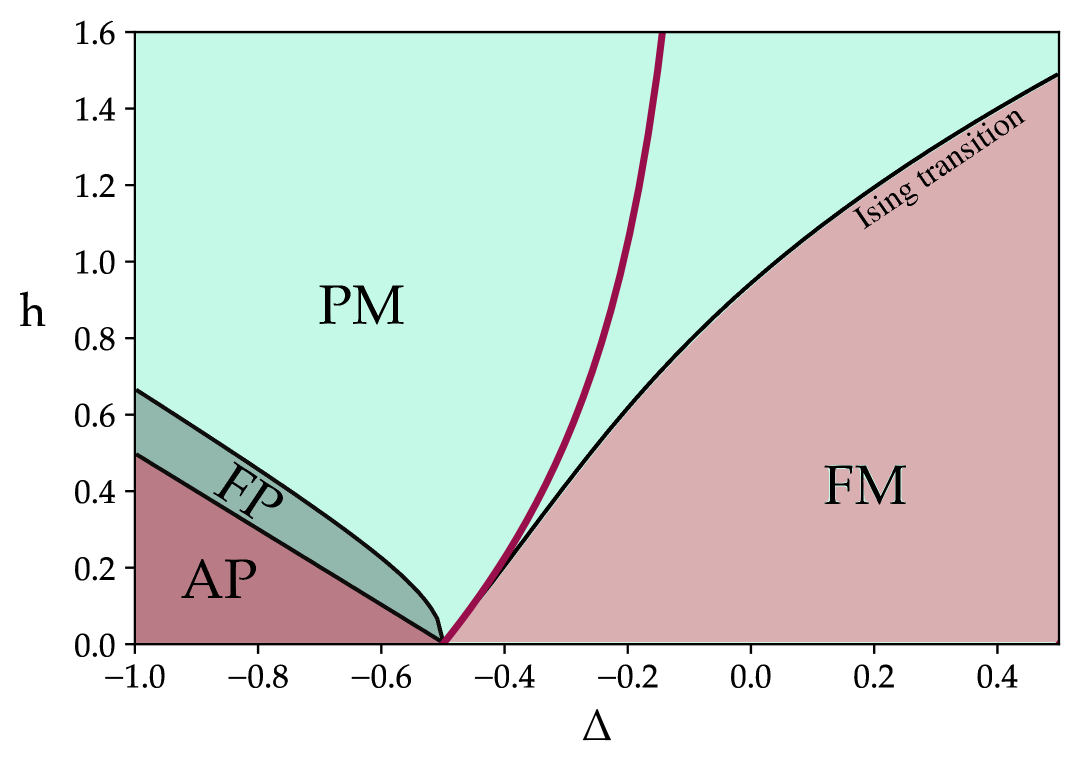
Figure 1: Phase diagram of the ANNNI model. The red line within the paramagnetic phase indicates the Peschel-Emery line. Adapted from [14].

The second model investigated in this work is a modification of the Transverse Field Ising Model, incorporating additional next nearest neighbour interactions. It is known as the Anisotropic or Axial Next Nearest Neighbour Ising Model and has been studied extensively in the last few decades [15, 16, 14, 7, 8]. Alongside the nearest neighbour coupling $J$ and the coupling $h$ to an external magnetic field, the interaction between next nearest neighbours can be tuned by a parameter $\Delta$ in the Hamiltonian [14]

$$H_{\mathrm{ANNNI}}=-J\sum_{j}\left(\sigma_{j}^{z}\sigma_{j+1}^{z}+\Delta\sigma_{j}^{z}\sigma_{j+2}^{z}+h\sigma_{j}^{x}\right).$$ (31)

This interaction strength $\Delta$ is also known as the “frustration” parameter [17]. The ANNNI model is the simplest model that incorporates quantum fluctuations (coupling $h$) and frustrated exchange interactions (coupling $\Delta$). As such, it serves as a fundamental model for exploring the dynamics between magnetic ordering, frustration, and disordering effects [17].

The competition between interactions gives rise to a more complex phase diagram, accommodating four different phases, as illustrated in Fig. 1. These phases are the paramagnetic (PM) phase, the ferromagnetic (FM) phase, a critical incommensurate floating phase (FP), and an anti-phase (AP).

In contrast to the TFIM the ANNNI model is not integrable [14], except along two lines in the phase diagram: the trivial line with $\Delta=0$ (that corresponds to the TFIM) and the so-called Peschel-Emery (PE) line [18]. The PE line is a disorder line along which the Hamiltonian factorises into local Hamiltonians $H_{j}^{\operatorname{loc}}$, such that it takes the form [19]

$$H_{\text{ANNNI}}^{\text{PE}}=\sum_{j}H_{j}^{\operatorname{loc}}.$$ (32)

The ground state of this factorised Hamiltonian is exactly degenerate and can be written as product states [20]. The model described by Eq. (32) is frustration-free, as the ground state of the full Hamiltonian $H_{\text{ANNNI}}^{\text{PE}}$ minimises each local Hamiltonian $H_{j}^{\operatorname{loc}}$ independently [19]. In the ANNNI model, the PE line is described by [18]

$$h=h^{*}:=\Delta-\frac{1}{4\Delta}.$$ (33)

The Hamiltonian of the ANNNI model can be mapped onto an interacting quantum Ising model by dual mapping and a subsequent rotation, resulting in the interacting quantum Ising Hamiltonian [20]. After further applying a Jordan-Wigner transformation, this Hamiltonian is equivalent to the Kitaev-Hubbard chain and the $XZ$ Heisenberg chain [20, 19, 21]:

$$\begin{split}H_{\text{ANNNI}}=&J\sum_{j=1}^{L}\bigg{(}h\left(c_{j}^{\dagger}-c_{j}\right)\left(c_{j+1}^{\dagger}+c_{j+1}\right)\\ &+\Delta\left(1-2c_{j}^{\dagger}c_{j}\right)\left(1-2c_{j+1}^{\dagger}c_{j+1}\right)-\left(1-2c_{j}^{\dagger}c_{j}\right)\bigg{)}.\end{split}$$ (34)

Due to the quartic interaction arising from the next-nearest neighbour coupling in the spin-$\frac{1}{2}$ system, the ANNNI model does not have a simple analytical solution like the TFIM.

The ground state along the PE line is a direct product state [19]:

$$|\text{GS}_{i}^{(\pm)}\rangle=\mathbin{\mathop{\otimes}\displaylimits_{j=1}^{L}}\frac{1}{\sqrt{(1\pm\alpha)^{L}}}\bigg{(}\left|\uparrow\right\rangle_{j}\pm\alpha\left|\downarrow\right\rangle_{j}\bigg{)},$$ (35)

where $\alpha=\sqrt{\cot{\left(\frac{\theta^{*}}{2}\right)}}$ with $\theta^{*}=\arctan{\left(h^{*}\right)}=\arctan{\left(\Delta-\frac{1}{4\Delta}\right)}$ [19]. We see that $\alpha\geq 1$ along the entire frustration-free line.

As a post-quench Hamiltonian we consider the model at $\mu=0$,

$$H_{0}=-t\sum_{j=1}^{L-1}\sigma_{j}^{x}\sigma_{j+1}^{x}.$$ (36)

The eigenstates of this Hamiltonian are simply products of the eigenstates of $\sigma_{j}^{x}$, namely

$$|\phi\rangle=\mathbin{\mathop{\otimes}\displaylimits_{j=1}^{L}}|\pm\rangle_{j},$$ (37)

and the ground states are

$$|+\rangle=\mathbin{\mathop{\otimes}\displaylimits_{j=1}^{L}}|+\rangle_{j}\quad\text{and}\quad|-\rangle=\mathbin{\mathop{\otimes}\displaylimits_{j=1}^{L}}|-\rangle_{j}.$$ (38)

Expressing $|\text{GS}_{i}^{(\pm)}\rangle$ in terms of $|\pm\rangle_{j}$ yields

$$|\text{GS}_{i}^{(\pm)}\rangle=\frac{1}{\sqrt{2^{L}}}\mathbin{\mathop{\otimes}\displaylimits_{j=1}^{L}}\bigg{(}(1\pm\alpha)|+\rangle_{j}+(1\mp\alpha)|-\rangle_{j}\bigg{)},$$ (39)

where we used

$$\left|\uparrow\right\rangle_{j} =\frac{1}{\sqrt{2}}\bigg{(}|+\rangle_{j}+|-\rangle_{j}\bigg{)}\quad\text{and}$$ (40)

$$\left|\downarrow\right\rangle_{j} =\frac{1}{\sqrt{2}}\bigg{(}|+\rangle_{j}-|-\rangle_{j}\bigg{)}.$$ (41)

The post-quench ground states are given by $|\phi_{0}^{+}\rangle=|\phi^{L}\rangle=\mathbin{\mathop{\otimes}\displaylimits_{j=1}^{L}}|+\rangle_{j}$ and $|\phi_{0}^{-}\rangle=|\phi^{0}\rangle=\mathbin{\mathop{\otimes}\displaylimits_{j=1}^{L}}|-\rangle_{j}$, whereas the post-quench excited states are given by $|\phi^{N}\rangle=\mathbin{\mathop{\otimes}\displaylimits_{j=1}^{N}}|+\rangle_{j}\mathbin{\mathop{\otimes}\displaylimits_{l=N+1}^{L}}|-\rangle_{l}$ and its permutations, where $N<L$. The resulting overlaps with the pre-quench ground state are

$$\bigg{|}\langle\text{GS}_{i}^{(\pm)}|\phi_{0}^{\pm}\rangle\bigg{|}^{2} =\frac{1}{2^{L}}\bigg{(}1\pm\alpha\bigg{)}^{2L}$$ (42)

for the ground state overlap, and

$$\bigg{|}\langle\text{GS}_{i}^{(\pm)}|\phi^{N}\rangle\bigg{|}^{2} =\frac{1}{2^{L}}(1\pm\alpha)^{2N}(1\mp\alpha)^{2(L-N)}$$ (43)

for the overlap of the pre-quench ground state with a post-quench excited state.

For the conjecture to hold, the ratio of these two overlaps should be smaller than one:

$$\bigg{|}\langle\text{GS}_{i}|\text{GS}_{f}\rangle\bigg{|}^{2}\overset{!}{>}\bigg{|}\langle\text{GS}_{i}|\tilde{\psi}\rangle\bigg{|}^{2}\Leftrightarrow\bigg{|}\frac{\langle\text{GS}_{i}|\tilde{\psi}\rangle}{\langle\text{GS}_{i}|\text{GS}_{f}\rangle}\bigg{|}^{2}\overset{!}{<}1.$$ (44)

We consider both ground states separately:

$$\begin{split}&\bigg{|}\frac{\langle\text{GS}_{i}^{+}|\phi^{N}\rangle}{\langle\text{GS}_{i}^{+}|+\rangle}\bigg{|}^{2}=\frac{(1+\alpha)^{2N}(1-\alpha)^{2(L-N)}}{(1+\alpha)^{2L}}\\ =&\frac{(1-\alpha)^{2(L-N)}}{(1+\alpha)^{2(L-N)}}=\bigg{(}\frac{1-\alpha}{1+\alpha}\bigg{)}^{2(L-N)}<1\forall\alpha_{i}>0\end{split}$$ (45)

$$\begin{split}&\bigg{|}\frac{\langle\text{GS}_{i}^{-}|\phi^{N}\rangle}{\langle\text{GS}_{i}^{-}|-\rangle}\bigg{|}^{2}=\frac{(1-\alpha)^{2N}(1+\alpha)^{2(L-N)}}{(1+\alpha)^{2L}}\\ =&\frac{(1-\alpha)^{2N}}{(1+\alpha)^{2(L-(L-N))}}=\bigg{(}\frac{1-\alpha}{1+\alpha}\bigg{)}^{2N}<1\forall\alpha_{i}>0\end{split}$$ (46)

In this calculation only the ground state overlaps $\langle\text{GS}_{i}^{+}|+\rangle$ and $\langle\text{GS}_{i}^{-}|-\rangle$ are considered, while $\langle\text{GS}_{i}^{+}|-\rangle$ and $\langle\text{GS}_{i}^{-}|+\rangle$ are not computed explicitly. This is due to the fact that the former expression is significantly larger than the latter. Further it should be mentioned that for calculating the overlap, only the number of flipped spins is relevant; the number of domain walls does not influence the result. Eigenstates that differ from an “ordered” excited state (e.g., $\left|\uparrow\uparrow\uparrow\uparrow\downarrow\downarrow\right\rangle$) may have more domain walls and, consequently, a different excitation energy. However, this does not affect the quantum mechanical overlap.

Equations (45) and (46) confirm that condition (44) is satisfied. Thus, the conjecture could be verified analytically for the special case of a quench originating along the frustration-free PE line and ending at the specific choice of the Hamiltonian given in Eq. (36).

V Numerical Analysis of the ANNNI model

To investigate the conjecture’s validity beyond this special case, we conducted a numerical analysis of the ANNNI model. We present results obtained through Exact Diagonalisation (ED). Given the constraints of the available computational resources, the largest accessible system size for these computations is $L=16$ spins. The presentation of the results is structured according to the phase diagram shown in Fig. 1. Each point in the phase diagram corresponds to a parameter combination that uniquely defines the post-quench Hamiltonian. For clarity and ease of interpretation, dashed lines are used to reconstruct the phase boundaries. The quench starting points are indicated in the title of each plot and marked by a star in the phase diagram. The results are displayed using a colour code based on the normalised deviation of the ground state overlap from the maximal overlap, defined as:

$$\text{deviation}=\frac{|\text{GS}\rangle\ \text{overlap}-\text{max. overlap}}{\text{max. overlap}}.$$ (47)

In this visualisation, a very bright teal colour indicates that the ground state overlap equals the maximal overlap, while darker colours signify a greater deviation between these two quantities.
Within the phase where the quench starts, all points should ideally be displayed in the brightest colour for the conjecture to hold true. Any darker colour within that phase indicates a violation of the conjecture, as it signifies that the maximal overlap is not provided by the ground state overlap in such cases.

[] [] []

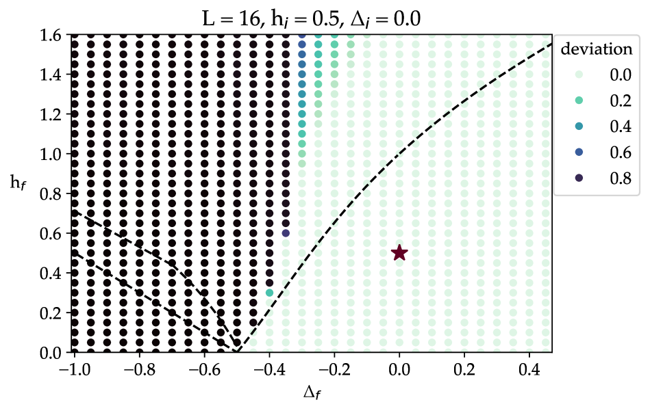
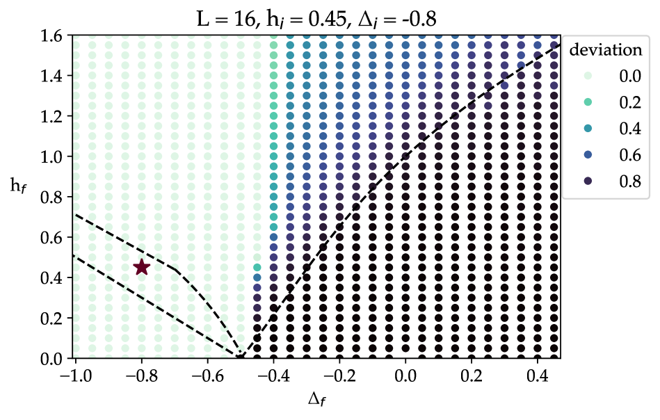
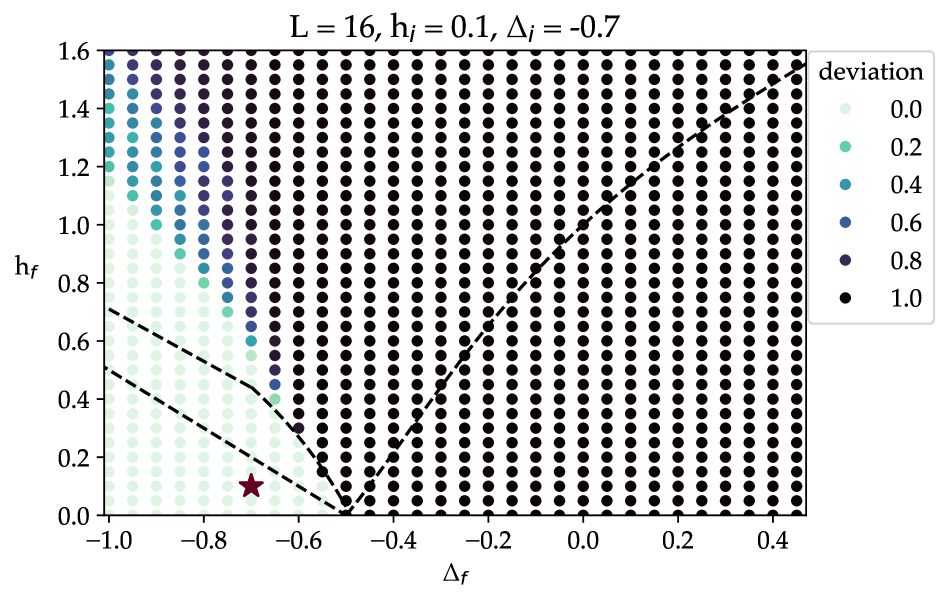
Figure 2: Quenches within the ferromagnetic (a), floating (b) and anti-phase (c).

For all tested quench configurations within the ferromagnetic, floating and anti-phase, the numerical data consistently support the conjecture. However, for pre-quench ground states in the paramagnetic phase, the numerical results are partly inconclusive.

Fig. 3 shows a starting point at $\Delta_{i}=-0.5$ successively approaching the quadruple point. When the quench starts far from this multiphase point, the numerical results support the conjecture. However, as the quench starting point moves closer to the quadruple point, violations of the conjecture begin to appear close to the Ising phase transition. Fig. 5 explores whether these violations could be caused by finite-size effects, as a shifted position of the phase boundaries for smaller systems is a known phenomenon in the ANNNI model [17].

[] [] [] []

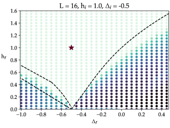
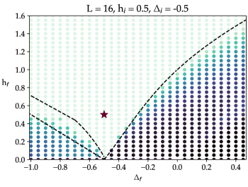
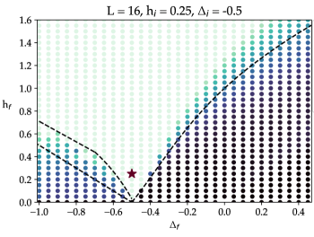
Figure 3: Quenches within the paramagnetic phase of starting point successively approaching the quadruple point.

The regions where the conjecture is violated become progressively smaller as the system size increases, suggesting that these violations might be due to finite-size effects. A more detailed investigation of this surmise can be conducted by computing the finite-size shifted locations of the phase transitions.

The concept of a “phase transition” is not well-defined in finite systems, particularly when the considered systems are very small. The term only applies to systems in the thermodynamic limit, where a phase transition is commonly characterised by a discontinuity in an order parameter. In contrast, at finite sizes, such discontinuities cannot be found, as it broadens to be a smooth extremum of the order parameter.

However, a quantity known as fidelity susceptibility has been shown to serve as an effective indicator of quantum phase transitions [22, 23, 24] as it quantifies the sensitivity of the ground state to perturbations. The fidelity susceptibility $\chi$ can be derived from Taylor expanding the fidelity $\mathcal{F}$ that is defined as [24]

$$\mathcal{F}(a,\delta a)=|\left\langle\text{GS}(a)\mid\text{GS}(a+\delta a)\right\rangle|,$$ (48)

where $a$ denotes a parameter of the Hamiltonian and $\delta a$ a small change in $a$. Its Taylor expansion reads [22]

$$\mathcal{F}(\delta a)=1-\frac{1}{2}\chi(\delta a)^{2}+\mathcal{O}\left((\delta a)^{3}\right).$$ (49)

The second order expansion coefficient sets the fidelity susceptibility $\chi$ to be

$$\chi=\frac{2}{(\delta a)^{2}}(1-\mathcal{F}).$$ (50)

[] [] []

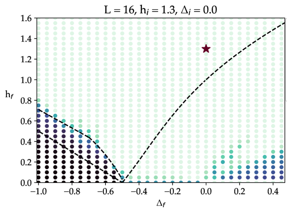
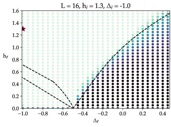
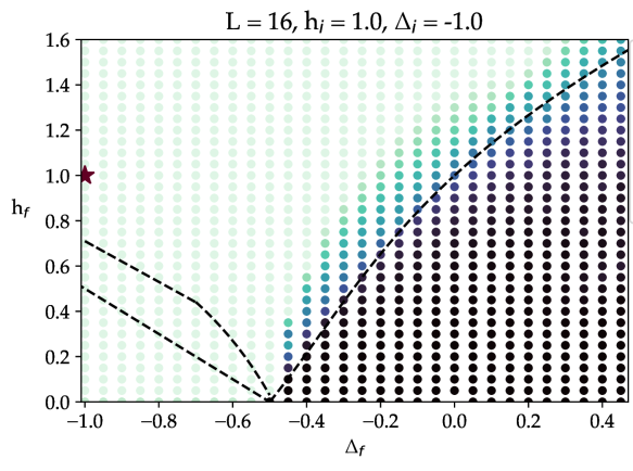
Figure 4: Other quenches within the paramagnetic phase showing violations of the conjecture.

The location of the phase transition found via this method identified using this method generally approaches the infinite-size phase transition asymptotically. The technique is applied in two directions, given that the phase diagram is two-dimensional: the shift in $h$ direction was determined while keeping $\Delta$ constant, and vice versa.

The “remodelled” phase boundaries for a system of $L=16$ spins are depicted in Fig. 6. We are aware that the fidelity susceptibility is not a reliable measure for tracking phase transitions near the floating phase, as it typically exhibits peak revivals that depend on the system size (cf. [25]).

Some violations, such as those illustrated in Fig.s 3 and 4, remain inexplicable by the adjusted positions of the phase transitions. However, other instances, such

[] [] []

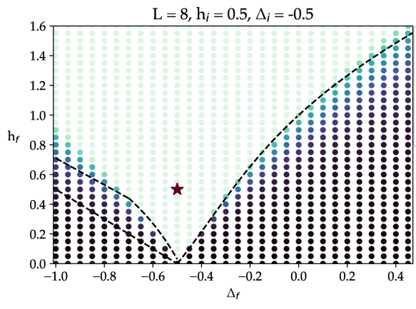
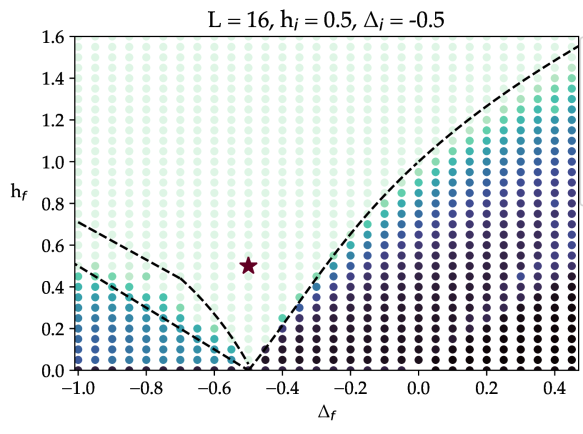
Figure 5: Quenches starting in the paramagnetic phase at $(\Delta,h)=(-0.5,0.5)$ for different system sizes.

as the quenches depicted in Fig.s 4, 5, and 5, can be accounted for by these revised phase transition locations.

VI Overlaps in Post-Quench Spectrum

For quenches within the same phase, the conjecture states that the largest overlap with the initial ground state should be that with the final ground state. Consequently, when plotting the overlaps against the post-quench Hamiltonian spectrum, the largest peak should align with the lowest energy state. In the following plots, we shifted the post-quench spectrum for this purpose such that the ground state energy is located at $0.0$ and all excitations energies are positive.

[] []

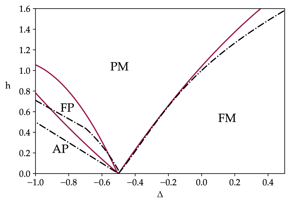
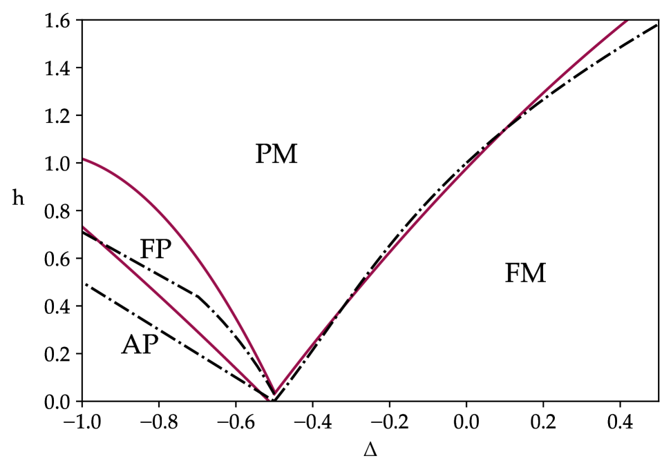
Figure 6: Finite-size shifted phase boundaries of the ANNNI model when keeping the parameters $h$ (panel 6) and $\Delta$ (panel 6) fixed, respectively. The dashed lines mark the DMRG-calculated phase boundaries of the infinite-sized system [14], while the red lines show the shifted transition lines.

Fig. 7 shows quenches within the paramagnetic phase, carried out along the depicted trajectories. The direction labelled “forward” denotes a quench from $i$ to $f$, while “backward” indicates a quench from $f$ to $i$. Quenches within the floating phase, anti-phase, and ferromagnetic phase are presented below using the same labelling scheme.

The results in Fig.s 7 to 10 were obtained employing exact diagonalisation. They support the conjecture, as the largest peak consistently occurs at the ground state energy.

This rendering of the results allows for a re-investigation of the quench depicted in Fig. 4, which fails to support the conjecture as points near the Ising transition exhibit a larger overlap than the ground state overlap. A parameter combination for the quench starting at the same point as in Fig. 4 and ending in the darker region close to the phase boundary is used for the result illustrated in Fig. 11.

[] [] []

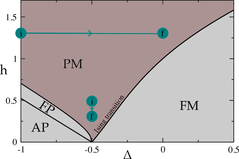
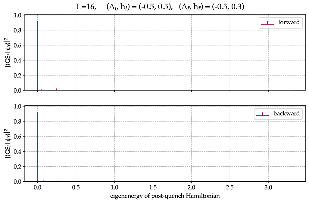
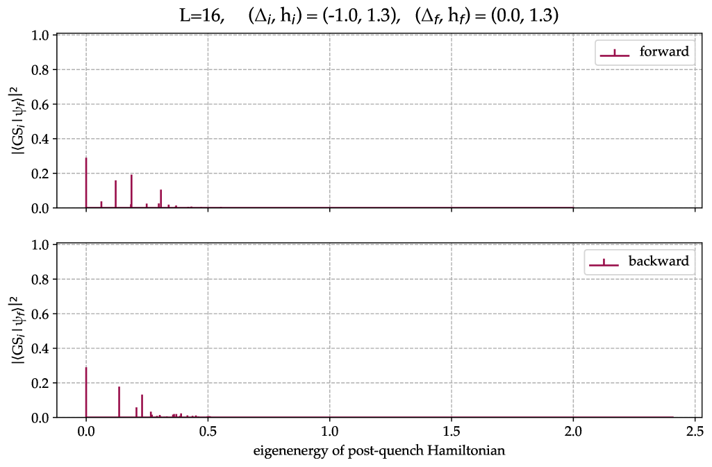
Figure 7: Quenches within the paramagnetic phase. The phase diagram in panel 7 shows the starting and ending points of the quenches. The quench from $i$ to $f$ is referred to as “forward”. Adapted from Karrasch et al. [14].

[] [] []

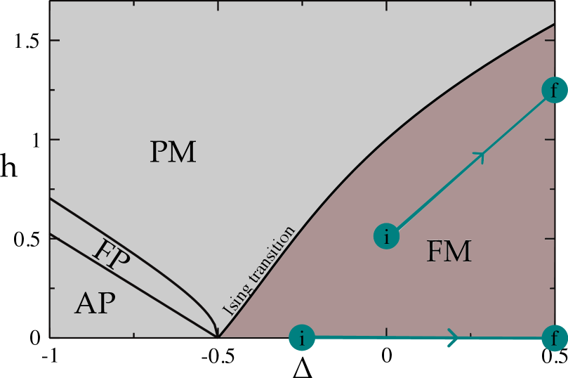
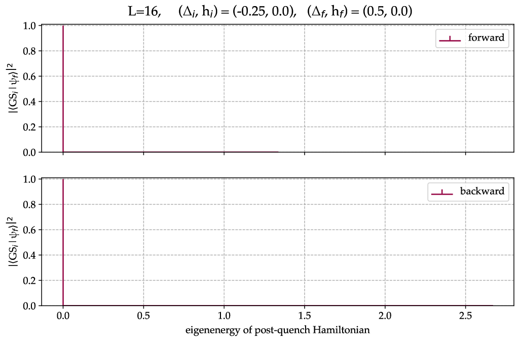
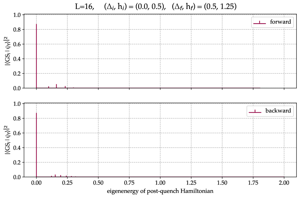
Figure 8: Quenches within the ferromagnetic phase. The phase diagram in panel 8 shows the starting and ending points of the quenches. The quench from $i$ to $f$ is referred to as “forward”. Adapted from Karrasch et al. [14].

[] []

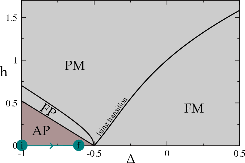
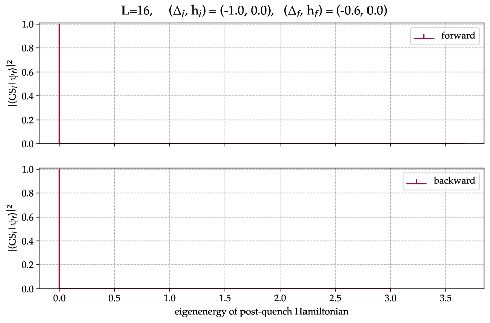
Figure 9: Quench within the anti-phase. The phase diagram in panel 9 shows the starting and ending points of the quench. The quench from $i$ to $f$ is referred to as “forward”. Adapted from Karrasch et al. [14].

[] []

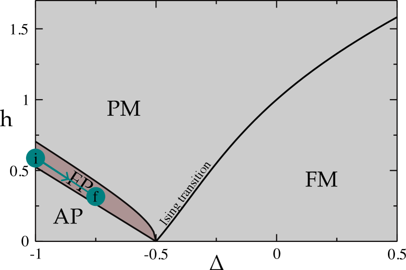
Figure 10: Quench within the floating phase. The phase diagram in panel 10 shows the starting and ending points of the quench. The quench from $i$ to $f$ is referred to as “forward”. Adapted from Karrasch et al. [14].

[] []

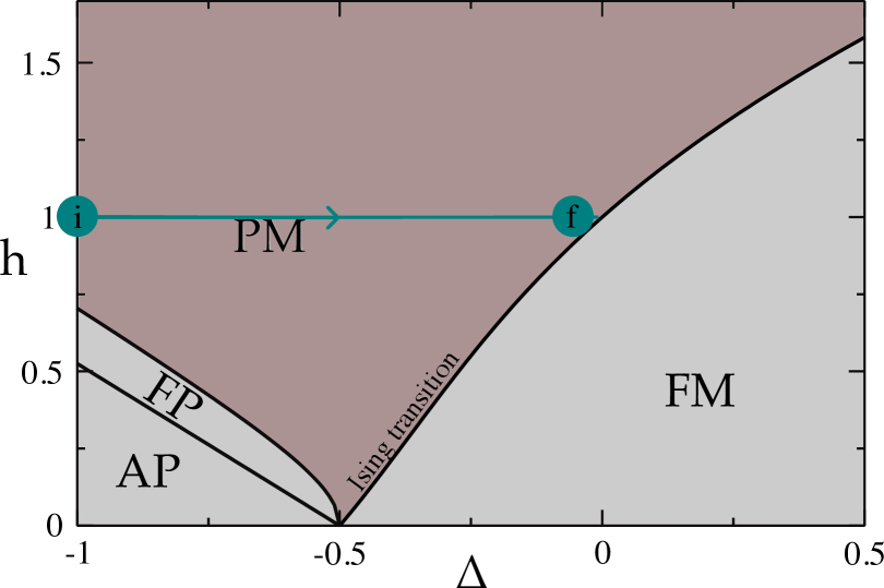
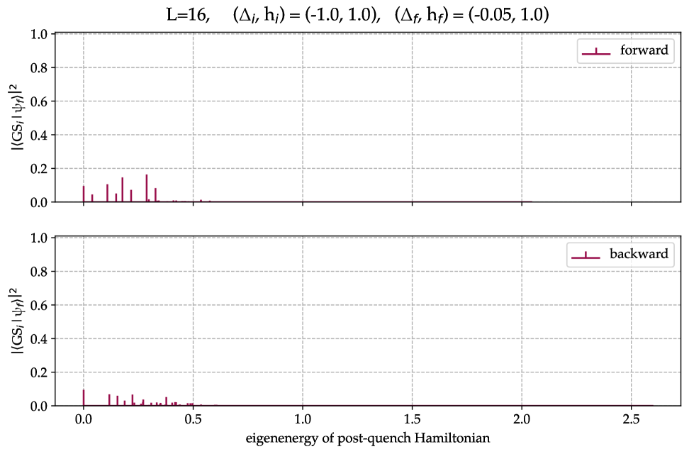
Figure 11: Quench within the paramagnetic phase showing ambiguous behaviour.

The result appears ambiguous: the backward quench supports the conjecture’s statement, whereas the forward result does not. In the upper panel of Fig. 11, the largest peak is not located at the ground state energy but at higher energies in the spectrum. In fact, the heights of three peaks exceed that of the ground state overlap. A possible however not certain explanation for this observation could be finite-size shifted phase boundaries that are shown in Fig. 6.

To demonstrate that the above results are not a generic feature of any quenched system, but rather provide support for the conjecture, we show some quenches across phase transitions in Appendix IX. For such quenches, the largest peak is likely to occur at higher energy levels. Appendix Figures 12, 13, and 14 show quenches across various phase boundaries of the ANNNI model that were carried out along the depicted trajectories.
In contrast to the quenches within the same magnetic phase, the maximum overlap does not align with the ground state energy. Exceptions to this observation arise for quenches between the anti-phase and floating phase as can be seen in Appendix Fig. 14. The finite-size shifted phase diagrams in Fig. 6 suggest that the anti-phase is extended to significantly higher values of $h$ for the finite systems studied and thus provide a possible explanation for why the anti-phase-floating phase transition is not traceable.

VII Conclusion

This work aimed to investigate the relationship between eigenstates of quenched Hamiltonians, specifically testing the validity of the conjecture formulated in Section II.
We conducted calculations in the TFIM and the ANNNI model. For the former, which is analytically solvable through Jordan-Wigner transformation and Bogoliubov rotation, we could establish a general analytical proof of the conjecture independent of specific quench points. For the ANNNI model, we could not attain a complete analytical proof as the model is not exactly solvable. Instead, we verified the conjecture in a special case where exact expressions for the pre- and post-quench ground states are available. To extend the analysis beyond this special case, we employed numerical methods.
The numerical analysis comprises ED and the Lanczos method to compute the Hamiltonian’s full spectrum or relevant parts of it. In the TFIM, numerical findings support the conjecture for all cases. Numerical results for the ANNNI model also mostly support the conjecture. While some violations could successfully be attributed to finite-size effects, for others it is not sure whether they can be explained with finite-size shifted phase boundaries. Employing other methods for quantifying finite-size effects may offer a more comprehensive explanation for the observed violations.
Overall, the findings cautiously affirm the conjecture, suggesting it as an extension of the adiabatic theorem by Born and Fock (1928)[10] to maximally non-adiabatic changes. We acknowledge that counterexamples can be constructed, at least for systems without a continuous spectrum. However, it remains unclear whether the conjecture holds universally for all systems with a continuous spectrum in the thermodynamic limit or if its validity must be restricted to a specific class of Hamiltonians or to quench end points that are relatively close to the quench start point. Further investigation is needed to determine the precise conditions under which the conjecture holds. Nevertheless, our results strongly suggest that a significant class of Hamiltonians satisfies the conjecture, making it worthwhile to explore the conditions under which it remains valid.

VIII Acknowledgement

We thank Dirk Schuricht for his valuable input, which contributed significantly to this paper. We acknowledge support from the Deutsche Forschungsgemeinschaft (DFG) through FOR 5522 (Project-ID 499180199).

IX Appendix

[] [] []

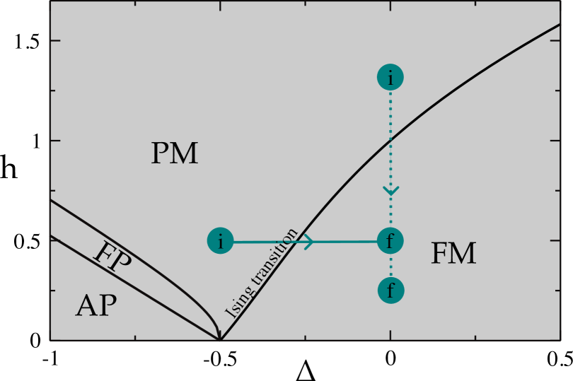
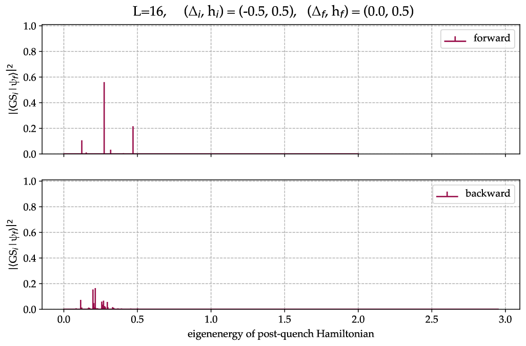
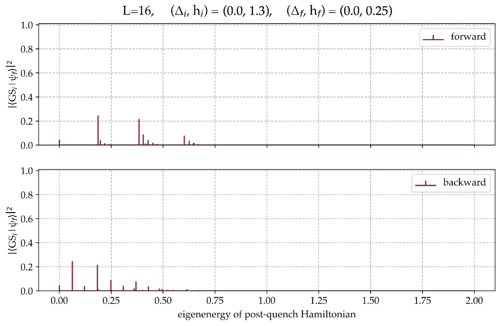
Figure 12: Quenches across the paramagnetic-ferromagnetic phase transition. The phase diagram in panel 12 illustrates the quench trajectories. The quench direction from $i$ to $f$ is referred to as “forward”. Adapted from Karrasch et al. [14].

[] [] []

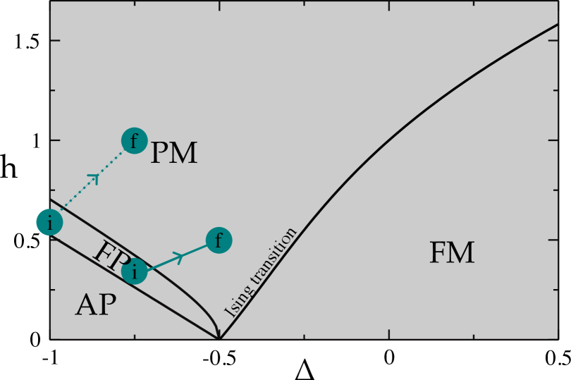
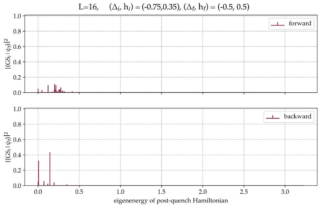
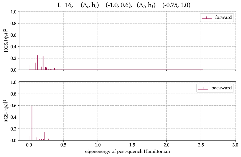
Figure 13: Quenches across the floating phase-paramagnetic phase transition. The phase diagram in panel 13 illustrates the quench trajectories. The quench direction from $i$ to $f$ is referred to as “forward”. Adapted from Karrasch et al. [14].

[] [] [] []

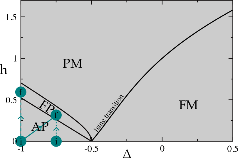
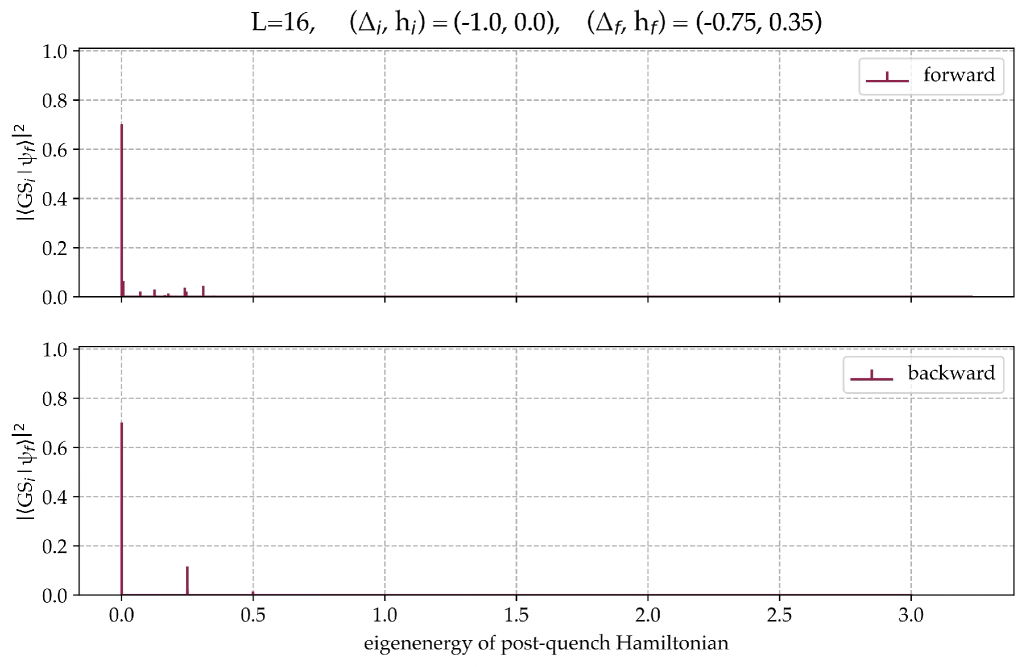
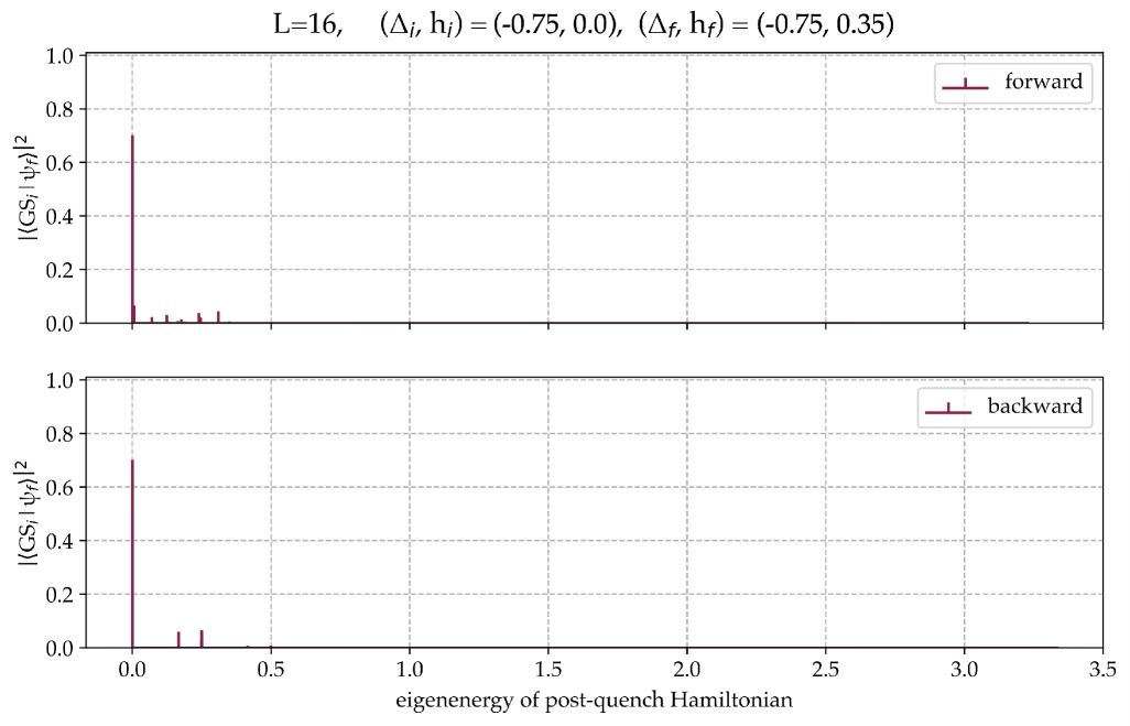
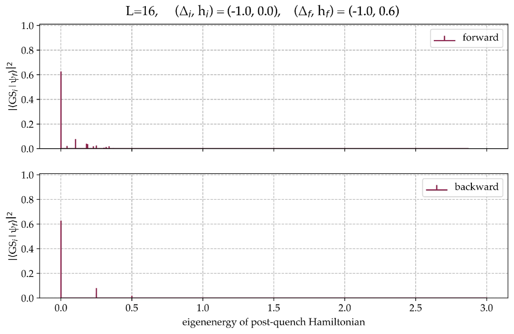
Figure 14: Quenches across the floating phase-anti-phase transition. The phase diagram in panel 14 illustrates the quench trajectories. Adapted from Karrasch et al. [14].

References

- Titum et al. [2019] P. Titum, J. T. Iosue, J. R. Garrison, A. V. Gorshkov, and Z.-X. Gong, Probing ground-state phase transitions through quench dynamics, Physical Review Letters 123, 10.1103/physrevlett.123.115701 (2019).
- Murayama et al. [2020] H. Murayama, Y. Sato, T. Taniguchi, R. Kurihara, X. Z. Xing, W. Huang, S. Kasahara, Y. Kasahara, I. Kimchi, M. Yoshida, Y. Iwasa, Y. Mizukami, T. Shibauchi, M. Konczykowski, and Y. Matsuda, Effect of quenched disorder on the quantum spin liquid state of the triangular-lattice antiferromagnet , Phys. Rev. Res. 2, 013099 (2020).
- Bloch et al. [2008] I. Bloch, J. Dalibard, and W. Zwerger, Many-body physics with ultracold gases, Rev. Mod. Phys. 80, 885 (2008).
- Trotzky et al. [2012] S. Trotzky, Y.-A. Chen, A. Flesch, I. P. McCulloch, U. Schollwöck, J. Eisert, and I. Bloch, Probing the relaxation towards equilibrium in an isolated strongly correlated one-dimensional bose gas, Nature physics 8, 325 (2012).
- Rossini and Vicari [2020] D. Rossini and E. Vicari, Dynamics after quenches in one-dimensional quantum ising-like systems, Phys. Rev. B 102, 054444 (2020).
- Gautam et al. [2024] M. Gautam, K. Pal, K. Pal, A. Gill, N. Jaiswal, and T. Sarkar, Spread complexity evolution in quenched interacting quantum systems, Phys. Rev. B 109, 014312 (2024).
- Haldar et al. [2021] A. Haldar, K. Mallayya, M. Heyl, F. Pollmann, M. Rigol, and A. Das, Signatures of quantum phase transitions after quenches in quantum chaotic one-dimensional systems, Phys. Rev. X 11, 031062 (2021).
- Robertson et al. [2023] J. H. Robertson, R. Senese, and F. H. L. Essler, A simple theory for quantum quenches in the ANNNI model, SciPost Phys. 15, 032 (2023).
- Heyl et al. [2018] M. Heyl, F. Pollmann, and B. Dóra, Detecting equilibrium and dynamical quantum phase transitions in ising chains via out-of-time-ordered correlators, Phys. Rev. Lett. 121, 016801 (2018).
- Born and Fock [1928] M. Born and V. Fock, Beweis des adiabatensatzes, Zeitschrift für Physik 51, 165 (1928).
- Silva [2008] A. Silva, Statistics of the work done on a quantum critical system by quenching a control parameter, Phys. Rev. Lett. 101, 120603 (2008).
- Jordan and Wigner [1993] P. Jordan and E. P. Wigner, Über das Paulische Äquivalenzverbot (Springer, 1993).
- Bogoljubov et al. [1958] N. N. Bogoljubov, V. V. Tolmachov, and D. V. Širkov, A new method in the theory of superconductivity, Fortschritte der Physik 6, 605 (1958).
- Karrasch and Schuricht [2013] C. Karrasch and D. Schuricht, Dynamical phase transitions after quenches in nonintegrable models, Physical Review B 87, 10.1103/physrevb.87.195104 (2013).
- Elliott [1961] R. J. Elliott, Phenomenological discussion of magnetic ordering in the heavy rare-earth metals, Phys. Rev. 124, 346 (1961).
- Fisher and Selke [1980] M. E. Fisher and W. Selke, Infinitely many commensurate phases in a simple ising model, Phys. Rev. Lett. 44, 1502 (1980).
- Cea et al. [2024] M. Cea, M. Grossi, S. Monaco, E. Rico, L. Tagliacozzo, and S. Vallecorsa, Exploring the phase diagram of the quantum one-dimensional annni model (2024), arXiv:2402.11022 [cond-mat.str-el] .
- Peschel and Emery [1981] I. Peschel and V. Emery, Calculation of spin correlations in two-dimensional ising systems from one-dimensional kinetic models, Zeitschrift für Physik B Condensed Matter 43, 241 (1981).
- Katsura et al. [2015] H. Katsura, D. Schuricht, and M. Takahashi, Exact ground states and topological order in interacting kitaev/majorana chains, Phys. Rev. B 92, 115137 (2015).
- Mahyaeh and Ardonne [2018] I. Mahyaeh and E. Ardonne, Exact results for a z3-clock-type model and some close relatives, Physical Review B 98, 10.1103/physrevb.98.245104 (2018).
- Sela and Pereira [2011] E. Sela and R. G. Pereira, Orbital multicriticality in spin-gapped quasi-one-dimensional antiferromagnets, Phys. Rev. B 84, 014407 (2011).
- Sierant et al. [2019] P. Sierant, A. Maksymov, M. Kuś, and J. Zakrzewski, Fidelity susceptibility in gaussian random ensembles, Phys. Rev. E 99, 050102 (2019).
- Zanardi and Paunković [2006] P. Zanardi and N. Paunković, Ground state overlap and quantum phase transitions, Phys. Rev. E 74, 031123 (2006).
- Wang et al. [2015] L. Wang, Y.-H. Liu, J. Imriška, P. N. Ma, and M. Troyer, Fidelity susceptibility made simple: A unified quantum monte carlo approach, Phys. Rev. X 5, 031007 (2015).
- Yu et al. [2022] X.-J. Yu, S. Yang, J.-B. Xu, and L. Xu, Fidelity susceptibility as a diagnostic of the commensurate-incommensurate transition: A revisit of the programmable rydberg chain, Physical Review B 106, 10.1103/physrevb.106.165124 (2022).