Universal Approximation Theorem for Deep Q-Learning via FBSDE System
Abstract
The approximation capabilities of Deep Q-Networks (DQNs) are commonly justified by general Universal Approximation Theorems (UATs) that do not leverage the intrinsic structural properties of the optimal Q-function, the solution to a Bellman equation. This paper establishes a UAT for a class of DQNs whose architecture is designed to emulate the iterative refinement process inherent in Bellman updates. A central element of our analysis is the propagation of regularity: while the transformation induced by a single Bellman operator application exhibits regularity, for which Backward Stochastic Differential Equations (BSDEs) theory provides analytical tools, the uniform regularity of the entire sequence of value iteration iterates—specifically, their uniform Lipschitz continuity on compact domains under standard Lipschitz assumptions on the problem data—is derived from finite-horizon dynamic programming principles. We demonstrate that layers of a deep residual network, conceived as neural operators acting on function spaces, can approximate the action of the Bellman operator. The resulting approximation theorem is thus intrinsically linked to the control problem’s structure, offering a proof technique wherein network depth directly corresponds to iterations of value function refinement, accompanied by controlled error propagation. This perspective reveals a dynamic systems view of the network’s operation on a space of value functions.
1 Introduction
Deep Reinforcement Learning (DRL) has achieved remarkable breakthroughs, with Deep Q-Networks (DQNs, see Mnih et al. (2015)) being a cornerstone. DQNs approximate the optimal action-value function, , using deep neural networks, enabling agents to learn effective policies in high-dimensional state spaces. The theoretical underpinnings of why DQNs can successfully represent often rely on general Universal Approximation Theorems (UATs) for neural networks Cybenko (1989); Hornik (1991). These theorems state that sufficiently large networks can approximate any continuous function on a compact set.
However, is not an arbitrary continuous function; it is the unique fixed point of a Bellman optimality operator, inheriting a rich structure from the underlying Markov Decision Process (MDP) dynamics, reward function, and discount factor. Standard UATs typically do not exploit this problem-specific structure. Moreover, while deep architectures like Residual Networks (ResNets, see He et al. (2016); Weinan et al. (2019); Li et al. (2022); Qi (2025)) are often employed and their depth is empirically crucial, the connection between depth and the approximation of is often qualitative (see Qi (2025)).
In continuous-time stochastic control, the optimal value function is known to be the (often unique) viscosity solution to a Hamilton-Jacobi-Bellman (HJB) PDE. This PDE frequently has a probabilistic representation via Backward Stochastic Differential Equations (BSDEs) when coupled with the forward state process (forming an FBSDE system, e.g., Peng (1992); El Karoui et al. (1997); Yong and Zhou (1999); Ma and Yong (1999)). These BSDE representations are known to yield important regularity properties (e.g., Lipschitz continuity) for the value function under appropriate assumptions on the coefficients of the dynamics and costs Pardoux (1999); Fleming and Soner (2006).
This paper aims to address this disparity by developing a UAT for a class of DQNs whose architecture is designed to reflect the iterative nature of Bellman updates. The proof technique leverages the propagation of regularity properties for the iterates of the Bellman operator. The transformation effected by a single Bellman step can be related to solving a short-horizon problem, whose value structure (and thus regularity) can be analyzed using tools related to BSDE theory. Crucially, the uniform regularity of all value iteration iterates (and the limit )—specifically, uniform Lipschitz continuity over a finite horizon—is a consequence of dynamic programming principles. Our contributions are:
-
1.
We frame the approximation of (the solution to a -discretized Bellman equation) not merely as function approximation, but as learning the limit of a dynamical system defined by the Bellman operator on a function space.
-
2.
We propose a DQN architecture where individual layers (or blocks of layers) are structured as neural operators. Each such operator block aims to approximate one step of the Bellman iteration, transforming a representation of the current Q-function iterate. Specifically, a block implementing aims for to approximate , where is the Bellman operator. This architecture establishes a structural correspondence between network depth and iteration count.
-
3.
We establish that the approximability of the Bellman operator (or its residual form ) by a neural operator block is predicated on the regularity of the functions it acts upon. Under standard Lipschitz and boundedness assumptions on the MDP coefficients (Assumption 2.1), the iterates of the Bellman operator converging to are shown to be uniformly Lipschitz continuous and uniformly bounded on their compact domain. This property ensures that the iterates reside within a compact subset of , a critical prerequisite for the application of neural operator UATs.
-
4.
Leveraging this uniform regularity, we develop a novel UAT proof where the network’s approximation of is achieved through a sequence of transformations mirroring the Bellman iterations. This iterative refinement approach, with controlled layer-wise error accumulation, provides a problem-aware justification for the approximation power of these specialized DQNs and demonstrates stable error propagation, contingent upon the neural operators satisfying certain stability properties (see Assumption 4.1).
This work offers a new perspective on the approximation capabilities of certain DQNs, particularly by highlighting how control-theoretic regularity ensures that the sequence of Bellman iterates forms a tractable set for approximation by neural operators, enabling an approximation framework structured around iterative refinement.
The paper is organized as follows. Section 2 introduces the continuous-time MDP, defines and , and briefly reviews BSDEs and the proposed DQN architecture. Section 3 outlines the core idea of representing through an iterative scheme with regularity arguments. Section 4 presents the main approximation theorem and a sketch of its proof, supported by key lemmas. Section 5 discusses potential for deeper results concerning quantitative approximation rates and the curse of dimensionality, and Section 6 concludes. Appendices A through D provide detailed proofs for the main lemmas and theorem, and further discussion on neural operators.
2 Preliminaries
2.1 Continuous-Time Markov Decision Process
Let be a filtered probability space supporting a -dimensional standard Brownian motion , where is a finite time horizon. We assume the filtration is the natural filtration generated by , augmented to satisfy the usual conditions. The state starting from at time evolves according to:
| (1) |
where is the action, chosen from a compact set . We consider policies that select an action at time (adapted to ) and hold it constant for a small duration , i.e., for . The functions (drift) and (diffusion) are specified in Assumption 2.1. The running reward rate is , and the terminal reward is . The continuous-time discount rate is .
Let be the compact state-time domain, and be the compact state-time-action domain. We consider functions . Let be the space of continuous functions on , equipped with the supremum norm .
Assumption 2.1 (MDP Coefficients and Rewards).
The state space and action space are compact sets. The time horizon is finite. Let and be points in . We define the metric (using Euclidean norms for ). There exist constants and such that for all :
-
•
The functions , , and are uniformly Lipschitz continuous on . Specifically:
-
–
.
-
–
. (Frobenius norm)
-
–
.
They are also bounded: , , . (Boundedness follows from Lipschitz continuity on a compact domain but stated for explicitness).
-
–
-
•
The terminal reward function is uniformly Lipschitz continuous on : . It is also bounded: .
-
•
The linear growth condition often assumed for SDE existence on unbounded domains, e.g., , is satisfied in a bounded form due to the compactness of .
Remark 2.2 (On Assumption 2.1).
The uniform Lipschitz continuity of with respect to and with respect to (Assumption 2.1) is crucial for ensuring that the optimal Q-function and all its Bellman iterates are uniformly Lipschitz continuous on the compact domain . This regularity is fundamental for the subsequent compactness arguments (Lemma 3.2) and the applicability of neural operator UATs (Lemma 4.3).111While strong, these assumptions are standard in stochastic control theory for establishing such regularity (e.g., Fleming and Soner (2006)). Relaxing these assumptions (e.g., to Hölder continuity or local Lipschitz conditions if domains were unbounded) would significantly complicate the regularity analysis and is beyond the scope of the current work, though an important direction for broader applicability. A detailed proof of Lemma 3.1 (d) (see Appendix A) explicitly shows how the uniform Lipschitz constant depends on the constants in Assumption 2.1 (such as , etc.), .
The optimal action-value function for the problem where controls are held constant for duration , is the unique fixed point in of the Bellman optimality equation:
| (2) |
where action is applied over , and . is the indicator function. For simplicity in some discussions, we might write assuming , but the full definition (2.1) handles the terminal boundary at . We assume is a multiple of for notational simplicity in iterative schemes where depth corresponds to time steps, but the definition of holds generally. The function is the value function for this specific -discretized control problem structure, representing the optimal expected discounted future reward over the entire horizon .
The function for a fully continuous control problem (not necessarily identical to derived from Eq. (2.1)) is the unique continuous viscosity solution to the Hamilton-Jacobi-Bellman (HJB) equation:
| (3) |
where .222The HJB equation is typically interpreted in the viscosity sense, as may not be everywhere. Our main analysis focuses on the Bellman equation (2.1) for . Under Assumption 2.1, is Lipschitz continuous (see Lemma 3.1 (d) and its proof in Appendix A). For existence and uniqueness of viscosity solutions to HJB equations under Lipschitz conditions on coefficients, see Fleming and Soner (2006).
2.2 Forward-Backward Stochastic Differential Equations (FBSDEs)
The solution to the HJB equation (3) can be characterized via BSDEs. If is an optimal feedback control for the continuous problem, then (where is the state under optimal control) solves the BSDE:
| (4) |
Here is related to . Such BSDE representations are fundamental in stochastic control theory Peng (1992); El Karoui et al. (1997); Yong and Zhou (1999) and are key to establishing regularity of . More direct relevance for this paper comes from using BSDEs to characterize the transformation performed by one step of the Bellman iteration for Eq. (2.1), as detailed in Section 3. This characterization helps establish the necessary regularity (Lipschitz continuity) of the function given regularity of .
2.3 Deep Q-Network Architecture (Operator-based ResNet)
We consider a Deep Q-Network that produces a sequence of Q-function approximations . Let be a finite discretization (grid) of . Let be an encoding operator, for . Let be a decoding operator (e.g., multilinear interpolation, kernel interpolation) that reconstructs a continuous function from its values on . The network aims to learn . Let be an initial estimate (e.g., ). The network consists of blocks, using a ResNet-like structure:
| (5) |
Here, is the function realized by the -th neural operator block. It is implemented as , where is a neural network (e.g., an MLP) parameterized by . This block aims for to approximate , where is the Bellman operator (defined in Sec. 3). Thus, aims to represent . The final Q-value approximation is . The overall parameters of the DQN are , and any parameters in if they are learned.333This architecture is specialized. The operator nature of acting on functions (approximated via on discretized representations) is crucial. Each layer refines the entire Q-function estimate. Architectures such as DeepONets Lu et al. (2021) or Fourier Neural Operators Li et al. (2021) provide frameworks for such operator learning, though here acts on finite-dimensional vectors representing function evaluations.
3 Optimal Q-function via an Iterative Scheme with BSDE-Inspired Regularity
Define the Bellman operator :
| (6) |
where action is fixed over , evolves via Eq. (1). The optimal Q-function is the unique fixed point of . Consider the sequence: (e.g., ), and . This sequence defines a discrete-time dynamical system on the Banach space , representing value iteration.
The computation of for a given can be related to a BSDE. Let be the forward state process (Eq. (1)) from under fixed action . The BSDE for on is:
| (7) | ||||
| (8) |
Then, . The existence, uniqueness, and regularity of (as a function of and properties of ) are standard results from BSDE theory. The driver . Under Assumption 2.1, is Lipschitz in , and is Lipschitz in (with coefficient ) and inherits Lipschitz continuity in from . The driver does not depend on . If is Lipschitz continuous in its arguments on , then its value is Lipschitz in because is compact. Consequently, the terminal condition (8) is Lipschitz in (or ) and depends regularly on . BSDE theory (e.g., Pardoux (1999) or El Karoui et al. (1997) for Lipschitz properties of with respect to initial data and parameters , given a Lipschitz driver and a Lipschitz terminal condition w.r.t. the forward state ) implies that will inherit Lipschitz continuity with respect to and appropriate regularity with respect to , provided is sufficiently regular. This BSDE perspective provides intuition for the regularity preservation of a single step . The uniform regularity for all value iteration iterates and (Lemma 3.1 (d)) is then established via an inductive argument on the finite horizon structure. We now state key properties of and the iterates .
Lemma 3.1 (Properties of and Iterates ).
Let Assumption 2.1 hold. Let be compact. Assume .
-
(a)
maps to . If is also Lipschitz continuous on (with Lipschitz constant ), then is also Lipschitz continuous on . Its Lipschitz constant depends on , , , the constants from Assumption 2.1, and . (This is established in detail as part of (d)).
-
(b)
is a contraction mapping on with contraction factor .
-
(c)
The value iteration sequence with (e.g., ) converges uniformly to the unique fixed point on .
-
(d)
If is Lipschitz continuous (e.g., ), then is Lipschitz continuous, and all iterates are uniformly bounded and uniformly Lipschitz continuous on . That is, there exists a constant , independent of , depending on , the constants in Assumption 2.1 (and implicitly the diameter of ), such that for any , is -Lipschitz, and consequently is also -Lipschitz.
Proof.
See Appendix A. ∎
Lemma 3.2 (Compactness of Iterates).
Under Assumption 2.1, if is Lipschitz continuous (e.g., ), the set of functions generated by value iteration is precompact in .
Proof.
This follows from Lemma 3.1 (d) (uniform boundedness and uniform Lipschitz continuity of all on the compact domain ). Uniform Lipschitz continuity implies equicontinuity. The Arzelà-Ascoli theorem then states that a set of functions that is uniformly bounded and equicontinuous on a compact domain is precompact in . ∎
4 Universal Approximation via FBSDE-Inspired Network Construction
We now formalize the UAT. The operator is central. Note . From Lemma 3.1 (b), , so is Lipschitz continuous with constant .
Assumption 4.1 (Properties of Neural Operator Class).
We assume the availability of a class of neural operators and a corresponding Universal Approximation Theorem (such as Kovachki et al. (2023); Chen and Chen (1995)) such that for any compact set consisting of functions uniformly Lipschitz with constant and uniformly bounded by , and any continuous operator where is also a set of uniformly Lipschitz functions (with constant and bound ), the following holds: For any , there exist , encoding/decoding operators , and a neural network (defining ) such that:
-
(a)
.
-
(b)
The function (for ) is Lipschitz continuous on for each . Moreover, there exists a uniform Lipschitz constant for the family of functions . This is determined by the choices of , , the architectural design of and , and potentially the characteristics () of the approximation task. Crucially for our analysis (see Remark 4.2), can be considered fixed once and the operator architecture achieving are determined for the set .
Remark 4.2 (On the determination of ).
Assumption 4.1 (b) is crucial for ensuring that the Lipschitz constants of the approximate iterates remain uniformly bounded. The constant arises from the specific architectural choices made to satisfy part (a). For instance, if has outputs whose components are bounded (e.g., , by design of for inputs from ), and reconstructs a function using fixed basis functions that are -Lipschitz (i.e., ), then . While is chosen based on and the regularity of functions in (characterized by ) and (characterized by ), the assertion is that once and the specific architectural constraints for and are fixed to achieve the approximation for this class , the resulting is determined by these fixed architectural properties. For the subsequent analysis of in Appendix C, this (associated with the neural operator chosen to approximate on ) is treated as a given constant. This avoids circularity where would depend iteratively on . This is a structural assumption on the neural operator class: it must be possible to construct operators that achieve good approximation while simultaneously ensuring their output functions have a controlled (non-exploding) Lipschitz constant. Further details are in Appendix D.
Lemma 4.3 (UAT for Neural Operators Approximating ).
Let Assumption 2.1 and Assumption 4.1 hold. Let be a compact set of functions satisfying specific boundedness and Lipschitz continuity properties (as defined by and in the proof of Theorem 4.4 in Appendix C, and shown therein to contain the iterates ). For any , there exist:
-
(i)
a sufficiently fine discretization grid of (i.e., large enough ), with corresponding encoding (e.g., point sampling) and decoding (e.g., multilinear interpolation or basis function expansion),
-
(ii)
a neural network (e.g., an MLP using activation functions satisfying Assumption 4.1, with sufficient capacity) with parameters ,
such that for any , if we define , then
and the function is -Lipschitz on , where is the constant from Assumption 4.1 (b) corresponding to the chosen , and the properties of the sets and . The required and capacity of may depend on the dimension of , potentially leading to the curse of dimensionality for grid-based methods.
Proof.
See Appendix B. ∎
Theorem 4.4 (UAT for DQNs via Iterative Refinement and Regularity Propagation).
Let Assumptions 2.1 and Assumption 4.1 hold. Let be the compact domain defined earlier. Assume . For any , there exist a number of operator layers (related to and ), a discretization scheme based on a sufficiently fine grid (where is fixed across layers, chosen based on and ), and parameters for the DQN architecture (5) (with each satisfying Assumption 4.1), such that the function satisfies
Proof.
See Appendix C. ∎
5 Quantitative Approximation Rates and Curse of Dimensionality
While Theorem 4.4 establishes existence, a quantitative analysis of approximation rates, particularly concerning the dependence on the dimensionality of the domain , is paramount for a complete understanding. Such an analysis requires delving into the geometric properties of the function spaces involved and the efficiency of their representation. This section outlines considerations for such an investigation.
5.1 Quantitative Approximation Rates
The overall approximation error is bounded by . The second term, , is the convergence error of value iteration, which is already quantitative:
Assuming , (uniform bound on from Lemma 3.1(d)). To achieve , we need . The first term, , depends on the per-step operator approximation error . From Appendix C (Step 2), . To make , we need . The challenge lies in quantifying the resources (discretization points , network complexity for ) needed to achieve this for approximating by . The error for a single operator block can be decomposed as:
Let . The second term is the interpolation error for . The first term can be bounded by if (as an operator ) is -Lipschitz (e.g., multilinear interpolation has for the sup-norm of grid values to sup-norm of function). This inner term is the error of the finite-dimensional network approximating the map .
5.1.1 Assumptions on Higher-Order Smoothness
To obtain explicit rates, one typically needs stronger regularity assumptions than just Lipschitz continuity (Lemma 3.1(d)). Suppose Assumption 2.1 is strengthened (e.g., are or ) such that the Bellman iterates and belong to a smoother function space, e.g., a Sobolev space or Hölder space for some . Proving such regularity for solutions of Bellman equations (related to HJB PDEs) is a substantial task, often requiring non-degeneracy conditions on and compatibility conditions at the boundary if has one (see, e.g., Krylov and Krylov (1987)). Let be the dimension of the domain .
5.1.2 Bounds on Discretization and Interpolation Error
If functions (and thus ) possess -order smoothness (e.g., partial derivatives up to order are bounded), then for standard interpolation schemes (like multilinear or spline interpolation) on a uniform grid with points, where the mesh size :
The constant would depend on the bounds of the -th order derivatives of , i.e., the norm of in . This directly impacts the term .
5.1.3 Bounds on Neural Network () Approximation Error
Let be the map , where . Or, more directly, aims to approximate . The complexity of approximating by (an MLP, for instance) depends on the properties of . If is sufficiently smooth as an operator, and its input functions are smooth, then might also exhibit some smoothness or structure. Standard results for MLP approximation (e.g., Yarotsky (2017); Barron (1993)) state that functions with certain regularity (e.g., in Sobolev or Besov spaces on ) can be approximated with a rate depending on the number of parameters (weights ) of the MLP. For example, for a function in , an error of might require parameters in general, which is again hit by CoD in . However, if the intrinsic dimension of the manifold is much smaller than , or if has specific compositional structure (e.g., if is a pseudo-differential operator or has other exploitable structure), better rates for might be achievable. The smoothness of as an operator between function spaces, e.g., from to , would be key here.
5.1.4 Overall Rate and Dependence on Parameters
Combining these, if is to be , then:
-
•
The interpolation error must be , implying .
-
•
The NN approximation error for must be . The number of parameters for would then depend on and . If classical rates apply, where is smoothness of the map on .
The total number of parameters would be roughly . This paints a picture where the CoD () heavily influences , and in turn heavily influences . Higher smoothness for mitigates the first CoD effect.
5.2 Implications for Mitigating the Curse of Dimensionality
5.2.1 Leveraging Smoothness for Advanced Discretization
If and indeed possess higher-order Sobolev or Besov regularity, one could move beyond uniform grids and simple multilinear interpolation.
-
•
Sparse Grids: For functions in certain Sobolev spaces (e.g., with bounded mixed derivatives, such as ), sparse grid techniques Bungartz and Griebel (2004) can achieve approximation errors of (for certain ) using points, where the exponent of is independent of (though constants and log factors depend on ). This would drastically improve the dependence on for the number of evaluation points . The UAT for would then apply to these coefficients.
-
•
Wavelet Approximations: Similar benefits can be obtained using adaptive wavelet approximations if functions exhibit sparsity in a wavelet basis, which is often linked to Besov space regularity .
Proving the required regularity ( with appropriate mixed derivative bounds or Besov regularity) from Assumption 2.1 (or strengthened versions) would be a major theoretical undertaking, likely involving techniques from parabolic PDE theory.
5.2.2 Potential for Non-Grid-Based Representations
The framework currently assumes a grid-based encoding . Deeper results might explore:
-
•
Spectral Methods: If is a simple domain (e.g., hypercube) and functions are very smooth (e.g., analytic or ), spectral expansions (e.g., Chebyshev or Fourier) could be used. The operator would then act on spectral coefficients. Fourier Neural Operators Li et al. (2021) are an example of this philosophy, effectively learning a Green’s function in Fourier space.
-
•
Low-Rank Tensor Approximations: If can be well-approximated by low-rank tensor formats (e.g., Tensor Train, Hierarchical Tucker) for high , then could be designed to operate within this manifold of low-rank tensors. This is a promising direction for high-dimensional problems but requires significant analytic and algebraic machinery (cf. Hackbusch (2012)).
-
•
Random Feature Maps / Kernel Methods: The encoding could be based on random features, connecting to kernel approximation theory and reproducing kernel Hilbert spaces (RKHS). The decoding would then be a linear combination of these features.
Each of these would require adapting Lemma 4.3 and its proof to the specific representation and proving that (or its iterates) interacts favorably with such structures, e.g., preserving low-rankness or sparsity in a given basis.
6 Conclusion and Contributions
This paper establishes a Universal Approximation Theorem (UAT) for a class of Deep Q-Networks (DQNs) by framing their operation as an iterative refinement process mirroring Bellman updates on function spaces. This problem-specific approach offers deeper insights than generic UATs. Our key contributions include:
-
1.
Iterative Refinement UAT: We develop a UAT where the DQN architecture (a deep residual network of neural operator blocks) emulates the Bellman iteration dynamics. Network depth directly corresponds to iteration count, linking architecture to the control problem’s solution process.
-
2.
Regularity Propagation as Foundation: A central technical achievement is proving that standard MDP coefficient regularity (Assumption 2.1) leads to uniform Lipschitz continuity and boundedness for the exact Bellman iterates and the optimal function (Lemma 3.1). This property, combined with the assumed capabilities of the neural operator class (Assumption 4.1, particularly the ability to produce approximants whose output functions possess a controlled Lipschitz constant ), ensures that the network-approximated iterates also exhibit uniform Lipschitz continuity and boundedness. This guarantees all relevant functions reside in a compact subset of , a critical condition for applying neural operator UATs (Lemma 4.3).
-
3.
Control-Theoretic Error Stability: The iterative structure facilitates a transparent error analysis. The overall approximation error is bounded by a sum of the value iteration truncation error (decreasing with depth ) and an accumulated per-layer operator approximation error, which remains stable due to the Bellman operator’s contractivity and the controlled nature of the neural operator blocks.
-
4.
New Perspective: We provide a dynamic systems view of DQNs operating on function spaces, offering a novel understanding of how network depth contributes to refining value function estimates.
This framework provides a new proof technique and a structured path for future investigations into quantitative approximation rates and strategies to mitigate the curse of dimensionality in DRL.
References
- Barron [1993] Andrew R Barron. Universal approximation bounds for superpositions of a sigmoidal function. IEEE Transactions on Information theory, 39(3):930–945, 1993.
- Bungartz and Griebel [2004] Hans-Joachim Bungartz and Michael Griebel. Sparse grids. Acta numerica, 13:147–269, 2004.
- Chen and Chen [1995] Tianping Chen and Hong Chen. Universal approximation to nonlinear operators by neural networks with arbitrary activation functions and its application to dynamical systems. IEEE transactions on neural networks, 6(4):911–917, 1995.
- Cybenko [1989] George Cybenko. Approximation by superpositions of a sigmoidal function. Mathematics of control, signals and systems, 2(4):303–314, 1989.
- El Karoui et al. [1997] Nicole El Karoui, Shige Peng, and Marie Claire Quenez. Backward stochastic differential equations in finance. Mathematical finance, 7(1):1–71, 1997.
- Fleming and Soner [2006] Wendell H Fleming and Halil M Soner. Controlled Markov processes and viscosity solutions, volume 25. Springer Science & Business Media, 2006.
- Hackbusch [2012] Wolfgang Hackbusch. Tensor spaces and numerical tensor calculus, volume 42. Springer, 2012.
- He et al. [2016] Kaiming He, Xiangyu Zhang, Shaoqing Ren, and Jian Sun. Deep residual learning for image recognition. In Proceedings of the IEEE conference on computer vision and pattern recognition, pages 770–778, 2016.
- Hornik [1991] Kurt Hornik. Approximation capabilities of multilayer feedforward networks. Neural networks, 4(2):251–257, 1991.
- Kelley [2017] John L Kelley. General topology. Courier Dover Publications, 2017.
- Kovachki et al. [2023] Nikola Kovachki, Zongyi Li, Burigede Liu, Kamyar Azizzadenesheli, Kaushik Bhattacharya, Andrew Stuart, and Anima Anandkumar. Neural operator: Learning maps between function spaces with applications to pdes. Journal of Machine Learning Research, 24(89):1–97, 2023.
- Krylov and Krylov [1987] Nikolai Vladimirovich Krylov and NV Krylov. Nonlinear elliptic and parabolic equations of the second order. Springer, 1987.
- Li et al. [2022] Qianxiao Li, Ting Lin, and Zuowei Shen. Deep learning via dynamical systems: An approximation perspective. Journal of the European Mathematical Society, 2022.
- Li et al. [2021] Zongyi Li, Nikola Borislavov Kovachki, Kamyar Azizzadenesheli, Burigede liu, Kaushik Bhattacharya, Andrew Stuart, and Anima Anandkumar. Fourier neural operator for parametric partial differential equations. In International Conference on Learning Representations, 2021. URL https://openreview.net/forum?id=c8P9NQVtmnO.
- Lu et al. [2021] Lu Lu, Pengzhan Jin, Guofei Pang, Zhongqiang Zhang, and George Em Karniadakis. Learning nonlinear operators via deeponet based on the universal approximation theorem of operators. Nature machine intelligence, 3(3):218–229, 2021.
- Ma and Yong [1999] Jin Ma and Jiongmin Yong. Forward-backward stochastic differential equations and their applications. Number 1702. Springer Science & Business Media, 1999.
- Mnih et al. [2015] Volodymyr Mnih, Koray Kavukcuoglu, David Silver, Andrei A Rusu, Joel Veness, Marc G Bellemare, Alex Graves, Martin Riedmiller, Andreas K Fidjeland, Georg Ostrovski, et al. Human-level control through deep reinforcement learning. In Nature, volume 518, pages 529–533. Nature Publishing Group, 2015.
- Oksendal [2003] Bernt Oksendal. Stochastic differential equations: an introduction with applications. Springer Science & Business Media, 2003.
- Pardoux [1999] Étienne Pardoux. Bsdes, weak convergence and homogenization of semilinear pdes. In Nonlinear analysis, differential equations and control, pages 503–549. Springer, 1999.
- Peng [1992] Shige Peng. Stochastic hamilton–jacobi–bellman equations. SIAM Journal on Control and Optimization, 30(2):284–304, 1992.
- Qi [2025] Qian Qi. Universal approximation theorem of deep q-networks. In International Conference on Machine Learning. PMLR, 2025. URL https://arxiv.org/abs/2505.02288.
- Weinan et al. [2019] E Weinan, Jiequn Han, and Qianxiao Li. A mean-field optimal control formulation of deep learning. Research in the Mathematical Sciences, 6(1):1–41, 2019.
- Yarotsky [2017] Dmitry Yarotsky. Error bounds for approximations with deep relu networks. Neural networks, 94:103–114, 2017.
- Yong and Zhou [1999] Jiongmin Yong and Xun Yu Zhou. Stochastic controls: Hamiltonian systems and HJB equations, volume 43 of Applications of Mathematics. Springer Science & Business Media, 1999.
Appendix A Proof of Lemma 3.1 (Regularity of Bellman Operator and Iterates)
We recall Assumption 2.1: The state space and action space are compact. The time horizon . The functions , , and are uniformly Lipschitz continuous on with constants respectively (using metric ). They are also bounded by . The terminal reward is -Lipschitz and bounded by . We assume .
Proof of Lemma 3.1.
Part (a): maps to . If is Lipschitz continuous on , then is also Lipschitz continuous on .
Let . The domain is compact, so is uniformly continuous and bounded. Let . Consider as defined in Eq. (3). Let be a sequence in converging to . Let denote the solution to the SDE Eq. (1) starting from with fixed action over . Let denote the solution starting from with fixed action over .
Under Assumption 2.1, and are uniformly Lipschitz in . Standard SDE theory (e.g., Yong and Zhou [1999] for stability with respect to initial data and parameters, or Oksendal [2003] ensuring conditions for these theorems are met by our Assumption 2.1) implies that for any :
where is an appropriate common time interval for comparison.444For instance, .
The integrand in the Bellman operator involves , , and . Since is continuous and bounded, is continuous and bounded, is continuous and bounded, and the state paths converge to in , and integration limits converge to , the Dominated Convergence Theorem can be applied. The terms are bounded by integrable constants (e.g., , , ). Thus, as . So, The argument for Lipschitz preservation is detailed in part (d).
Part (b): is a contraction mapping on with contraction factor .
Let .
If , the terms involving (related to continuation value) vanish from this part of the expression (the term is common to both). Taking the supremum over :
Since , we have . Thus, is a contraction.
Part (c): The sequence converges uniformly to .
Since is a Banach space (a complete metric space) and is a contraction mapping from to itself by part (b), the Banach Fixed-Point Theorem guarantees that has a unique fixed point , and for any , the sequence converges uniformly to . That is, .
Part (d): The optimal Q-function is Lipschitz continuous. If is Lipschitz, then each is Lipschitz, and are uniformly Lipschitz with constant . Consequently, is also -Lipschitz.
Uniform Boundedness of Iterates and : The function is the value function for a finite horizon problem. A standard bound for under Assumption 2.1 is if , or if . More simply, (for ). Let be this uniform bound for . If , then . If , then standard estimates for the Bellman operator (using its monotonicity and the fact that it maps constants to constants related to rewards) show that if , then involves . Iterating this, or using the contraction property , implies . If , then . A tighter argument: since preserves the property of being bounded by (if is so bounded, e.g., and ), all are uniformly bounded by .
Lipschitz Continuity of and Iterates by Induction: Let be -Lipschitz. (If , then .) Assume is -Lipschitz on . We want to show is -Lipschitz. Let and . Recall . Let be the solution for SDE Eq. (1) with fixed action over where . Let be the solution for SDE with fixed action over where .
SDE Stability Estimate: Under Assumption 2.1, are uniformly Lipschitz. Standard SDE estimates (e.g., Yong and Zhou [1999], or Fleming and Soner [2006]) ensure that for any fixed time horizon (here or ), there exists a constant , depending on , such that:
| (9) |
where is the evaluation time point (e.g., or ), and typically involves from Gronwall’s inequality. For comparing and , one often considers a common maximal interval.
Let . If is -Lipschitz in , then is -Lipschitz w.r.t. because is compact (standard result for sup over compact set).
Let . We analyze . Assume for simplicity and . Other cases (terminal conditions) are handled similarly and contribute terms of similar structure.
Term 1 (Integral part): Let . The difference can be bounded. This involves handling shifted integration limits and differences in the integrand due to vs . The Lipschitz continuity of , , and the SDE stability estimate (Eq. (9)) yield a bound of the form . depends on . For example, a component is .
Term 2 (Continuation value part): Let (assuming ).
If the terminal reward is used ( case), the term is . This contributes (not multiplied by ), with depending on .
Combining these parts, we obtain a recurrence for the Lipschitz constant of :
where:
-
•
collects all terms not multiplied by . It depends on , and SDE stability constants . is a finite positive constant.
-
•
. Note that depends on . is a finite positive constant.
The fixed point must satisfy . If , then . If , this fixed point argument does not directly yield a bound. However, is the value function of a finite-horizon problem (up to ). Standard results in stochastic control theory (e.g., from analysis of HJB equations or by backward induction on discrete time stages ) state that is Lipschitz continuous on under Assumption 2.1 (see, e.g., Fleming and Soner [2006]). Let be this true Lipschitz constant of . The value iterates converge to . If is -Lipschitz, the sequence is given by . Even if , since uniformly, and is -Lipschitz, the set is compact in by Lemma 3.2 (if is Lipschitz). This implies the must be uniformly bounded. The argument in Fleming and Soner [2006] for finite horizon problems often uses a backward induction. For (effectively), which is -Lipschitz. Then one shows is Lipschitz, and so on, back to . The maximum Lipschitz constant encountered over these stages would be . This effectively means that the number of "relevant" recursions for is bounded by . Thus is uniformly bounded for all by (assuming is the Lipschitz constant of , adjusted for -function structure, or if starting from ). This is finite. Thus, all (for ) and are uniformly -Lipschitz. ∎
Appendix B Proof of Lemma 4.3 (UAT for Neural Operators Approximating )
We want to show that for any , there exist , , and such that for any ,
and (as a function ) is -Lipschitz. The set is defined in the proof of Theorem 4.4 (Appendix C) as the set of functions that are -Lipschitz and uniformly bounded by .
Proof of Lemma 4.3.
1. Properties of and the set :
-
•
The set : As established in the proof of Theorem 4.4 (Step 3, Appendix C), the iterates (for ) are uniformly bounded by and uniformly -Lipschitz. The set
is compact in . The domain is compact. By the Arzelà-Ascoli theorem (e.g., [Kelley, 2017, Chapter 7, Theorem 17]), a set of functions in that is uniformly bounded and equicontinuous is precompact. The uniform -Lipschitz condition implies equicontinuity. is also closed in . Since is a complete metric space, a closed and precompact subset is compact.
-
•
The operator : Defined as , it maps . From Lemma 3.1 (b), is Lipschitz with constant . The identity operator is Lipschitz with constant 1. Thus, is Lipschitz continuous:
Since is Lipschitz continuous, it is continuous.
-
•
The image set : The set is compact in because it is the image of a compact set under a continuous map .
-
•
Regularity of functions in : Functions in are uniformly bounded and equicontinuous (hence uniformly Lipschitz) because is compact. Let be this uniform Lipschitz constant. Specifically, if is -Lipschitz, then is -Lipschitz (from Appendix A, using ). So is -Lipschitz, i.e., .
2. Application of Universal Approximation Theorem for Neural Operators (Assumption 4.1): We apply Assumption 4.1 with (whose functions are -Lipschitz and bounded by ) and . The image set consists of functions that are -Lipschitz and correspondingly bounded. The conditions for Assumption 4.1 are met:
-
(i)
The input domain for the operator, , is compact and consists of uniformly -Lipschitz and uniformly -bounded functions.
-
(ii)
The operator to be approximated, , is continuous from to . Its image is compact and consists of uniformly -Lipschitz functions.
Let be given.
-
•
Assumption 4.1 (a) implies that there exist , , and such that the composed operator satisfies
The choice of (and subsequently ) depends on and the properties of and (specifically their Lipschitz constants and bounds, which define their compactness and modulus of continuity).
-
•
Assumption 4.1 (b), as clarified in Remark 4.2, ensures that for the chosen and constructed (which achieve the approximation for functions in ), the function is Lipschitz continuous on with a uniform Lipschitz constant . This is a characteristic of the chosen approximating architecture for the given task (approximating on to accuracy ).
The proof of such UATs (e.g., as outlined in Kovachki et al. [2023] or Chen and Chen [1995], and strengthened by our Assumption 4.1 (b) regarding Lipschitz control) typically involves decomposing the total error:
| (E1) | ||||
| (E2) |
-
•
The term (E2) is the error from discretization and reconstruction of the target function . Since functions in are uniformly -Lipschitz, this error can be made arbitrarily small (e.g., ) by choosing sufficiently large (so the mesh size of the grid is small). For instance, for multilinear interpolation, the error is .
-
•
The term (E1) can be bounded by if is -Lipschitz as an operator from (with sup norm) to (with sup norm). For example, for multilinear interpolation. The inner term (where and for whose samples on are ) is made small by the UAT for the finite-dimensional network approximating the continuous map on the compact set . This error can be made small enough (e.g., such that ) by choosing with sufficient capacity. The Lipschitz property of the function (with constant ) is guaranteed by Assumption 4.1 (b).
∎
Appendix C Proof of Theorem 4.4 (UAT for DQNs via Iterative Refinement and Regularity Propagation)
Proof of Theorem 4.4.
Let be given. Let . The proof proceeds in four steps.
Step 1: Determine Number of Iterations/Layers . By Lemma 3.1(c), uniformly. The rate of convergence is given by:
Since , . From Lemma 3.1(d), is uniformly bounded by . So, . We choose such that the truncation error . This requires . Thus, we set (or if ). This is finite.
Step 2: Determine Per-Layer Approximation Accuracy for Neural Operator. Let . The network iterates are defined by . Let be the function representing the per-step operator approximation error at layer . So, . Then, . Let be the accumulated error up to layer . We have . The error propagates as:
If we can ensure for all , then by unrolling the recurrence:
We require the accumulated approximation error . So, we set the target per-layer operator error such that:
(If is small, one can use the exact sum . Then .) This since and .
Step 3: Define Compact Set , Show Iterates Belong to it, and Apply Lemma 4.3. To apply Lemma 4.3 uniformly for each layer , we need to show that all iterates belong to a common compact set . This involves showing uniform boundedness and uniform Lipschitz continuity for the sequence .
Uniform Boundedness of : From Lemma 3.1(d), the exact iterates are uniformly bounded by . The error for all . Thus, . Let . All (for ) are uniformly bounded by .
Uniform Lipschitz Continuity of : Let be the Lipschitz constant of as a function on . We have . From the proof of Lemma 3.1(d), if a function is -Lipschitz, then is -Lipschitz, where are constants defined therein (). The operator . If is -Lipschitz, then is -Lipschitz. Let this be .
According to Lemma 4.3 (which invokes Assumption 4.1), for the chosen per-layer error target (used as in Lemma 4.3), and for the (eventually defined) compact set , there exist , and neural networks such that for any :
-
(a)
.
-
(b)
The function is -Lipschitz on . Here, is the Lipschitz constant associated with the chosen neural operator architecture that achieves the -approximation for functions in when approximating . As per Assumption 4.1(b) and Remark 4.2, is treated as a fixed constant determined by these architectural choices (for the given and ) when analyzing the recurrence for .
The error function . If is -Lipschitz, then its image is -Lipschitz. The function is -Lipschitz. Therefore, is -Lipschitz, i.e., .
The recurrence for is derived from : . Let and . Since and (as a Lipschitz constant), we have . The recurrence is . Starting with : In general, . If (i.e., ), then . If , then . The iterates are considered for as inputs to the neural operator blocks. The maximum here is . Thus, their Lipschitz constants are uniformly bounded by , defined as:
This is finite since are finite, and is a fixed constant for the chosen architecture.
We now formally define the target compact set:
This set is compact in by Arzelà-Ascoli, as argued in Appendix B. We verify by induction that for .
-
•
Base case (): , so , and (true for ). Thus .
-
•
Inductive step: Assume for some . Thus its Lipschitz constant . More precisely, (or if ). Then Lemma 4.3 can be applied to with as input (since ). This guarantees existence of (chosen once based on , ) and for such that conditions (a) and (b) above hold (sup-norm error , output is -Lipschitz). Then . We already know . Its Lipschitz constant . Since (or if ), it follows that (or ). As , this implies . So .
This inductive argument confirms that all iterates for (which are inputs to the operator blocks) belong to the same compact set . The choice of and the properties of the neural operator class (including ) are thus consistently defined for this set. For each layer , we choose specific parameters for according to Lemma 4.3 to ensure .
Step 4: Final Error Bound. The total error for is:
This is . From Step 1, . From Step 2 (with justification from Step 3 that is achievable for all layers operating on inputs from ), . Therefore,
This completes the proof. ∎
Appendix D Further Details on Neural Operators and Function Representations
This appendix provides supplementary context on neural operators and function representations relevant to the main arguments, particularly concerning Assumption 4.1.
D.1 Neural Operators and Function Spaces
A neural operator is a mapping between function spaces (e.g., , ), parameterized by neural network weights . In our setting, the operator block is structured as:
The components are:
-
•
: An encoding operator, typically point sampling on a fixed grid , so .
-
•
: A standard neural network, such as a Multi-Layer Perceptron (MLP), parameterized by .
-
•
: A decoding operator that reconstructs a continuous function from its discrete values, e.g., using multilinear or higher-order polynomial interpolation, or a learned decoder.
Assumption 4.1 encapsulates the properties needed for our main theorem.
- 1.
-
2.
Lipschitz Property of Approximant Function (Assumption 4.1 (b)): This is critical for the stability of Lipschitz constants of . It requires that the constructed function itself be Lipschitz on , with a uniformly bounded Lipschitz constant . As detailed in Remark 4.2, is determined by the specific choices of , , and the architecture used to implement (e.g., properties of and ). The key is that for a given approximation task defined by on a set , an architecture can be chosen that both meets the accuracy requirement (a) and yields an output function with a certain Lipschitz constant . This then becomes a parameter of the chosen operator design for that task. For instance, if uses fixed -Lipschitz basis functions and is constructed to have outputs bounded by (e.g., through bounded weights or activation functions), then . While depends on the regularity of (e.g., ) to achieve , the argument is that once and other architectural constraints () are fixed to satisfy (a), is determined by these choices. It is this fixed (associated with the specific operator constructed for the approximation task on ) that is used in the recurrence for .
The existence of such an (uniform for and ) is essential. This is a stronger requirement than basic UATs for NOs but is considered architecturally achievable by design.
D.2 Function Representation and Discretization Error
The choice of the discretization grid and the interpolation scheme directly impacts the reconstruction error term for .
-
•
If functions are -Lipschitz (as established for ) on (a compact domain of dimension ), then standard multilinear interpolation on a uniform grid with mesh size yields an error of .
-
•
If functions possess higher smoothness (e.g., are with bounded -th derivatives), the error can be .
To achieve an interpolation error component of , might need to be of the order (where for Lipschitz functions). This dependence on highlights the curse of dimensionality (CoD) concerning the required number of grid points . While the CoD does not invalidate the UAT’s existence claim (which is generally non-quantitative in for generic NO-UATs unless specific rates are proven for the operator class and function regularity), it underscores practical challenges for approximating functions in high-dimensional spaces using grid-based methods. This is further discussed in Section 5.
D.3 Example UAT for Neural Operators
References such as Chen and Chen [1995] or Kovachki et al. [2023] provide the theoretical foundation for Lemma 4.3 (a).
-
•
For instance, Kovachki et al. [2023] states that for a continuous operator , where is a compact subset of , and for any , there exists a neural operator (belonging to a specific class, e.g., Graph Kernel Network based, or FNO-like) such that .
-
•
The architecture can be viewed as a specific realization of such a neural operator. This is particularly clear when employs a set of basis functions and computes the coefficients for these basis functions. The DeepONet architecture Lu et al. [2021] also fits this general framework and has its own UAT.
Assumption 4.1 (b) extends these typical UATs by requiring control over the Lipschitz constant of the output function , not just the Lipschitz constant of the operator itself (mapping function to function in sup-norm). This is justified by constructing to be Lipschitz as a map and to have bounded outputs, and choosing a decoder that translates these properties into a controlled Lipschitz constant for the resulting function on .
Appendix E Illustrative Example of Bellman Iteration and Regularity
This appendix provides a highly simplified example to illustrate the iterative application of the Bellman operator and the concept of regularity propagation, as discussed in Section 3 and Lemma 3.1. This example is purely pedagogical and does not involve neural network approximation, but its dynamics can be visualized.
Consider a one-dimensional continuous state space . Let the action space be discrete, , representing "move left" and "move right". The dynamics are deterministic. For a state and a small step size :
-
•
Action : .
-
•
Action : .
Let the immediate reward be . This reward is bounded () and Lipschitz continuous on (e.g., , so ). Let the discount factor be . We consider a finite horizon of "steps to go". The value functions are iterates, where represents the number of steps of Bellman updates performed, starting from an initial guess. is the initial guess, and is the Q-function after updates. For this example, , so we compute . Here, will be the optimal Q-function for a problem that lasts two stages from the current decision point.
The Bellman iteration for from is:
where is the state resulting from taking action in state .
Iteration (Initial Q-function):
This function is trivially bounded (by ) and Lipschitz continuous (with ). Numerical computation confirms is identically zero (Figure 1, top panel).
Iteration : Since , we have:
Note that is independent of in this case.
-
•
Boundedness: .
-
•
Lipschitz Continuity: As is -Lipschitz, is -Lipschitz with respect to . It is constant (and thus -Lipschitz) with respect to .
Numerical computation confirms with negligible error (max absolute difference of from the analytic form). This is visualized in Figure 1 (middle panel), where both action curves overlap.
Iteration (Q-function after two updates): Let and . The term becomes , where . So, is:
-
•
Boundedness: Since and are bounded, is clearly bounded. For example, .
-
•
Lipschitz Continuity (w.r.t. ): The function is -Lipschitz. The function is -Lipschitz on . The composition is -Lipschitz. Thus, is a sum of (-Lipschitz) and (-Lipschitz). Its Lipschitz constant w.r.t. is bounded by . A similar argument holds for .
Numerical computation yields values that match these analytical forms with very small differences (max absolute difference of approximately ), primarily due to interpolation of values when falls between discretized state points. The distinct shapes for and are visible in Figure 1 (bottom panel).
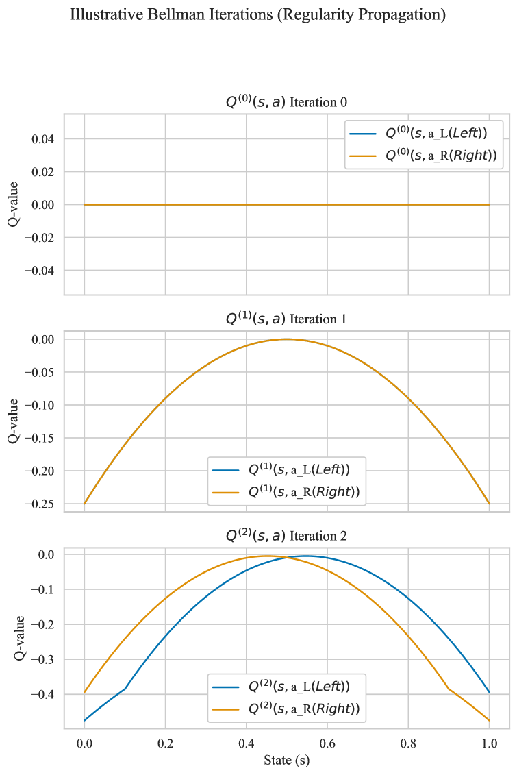
This simple example, supported by the numerical results and Figure 1, demonstrates:
-
1.
The iterative nature of the Bellman operator, transforming an initial Q-function estimate.
- 2.
-
3.
The functions are well-behaved (continuous, Lipschitz) under standard assumptions on rewards and dynamics, even with the operations.
While highly simplified, it captures the essence of the function sequence converging to within a space of regular functions.