Mixed-Integer Optimization for
Responsible Machine Learning

Justin, Sun, Gómez, and Vayanos

Mixed-Integer Optimization for Responsible Machine Learning

Nathan Justin Center for Artificial Intelligence in Society and Department of Computer Science, University of Southern California, Los Angeles, California 90089, USA, njustin@usc.edu Qingshi Sun Center for Artificial Intelligence in Society and Department of Industrial & Systems Engineering, University of Southern California, Los Angeles, California 90089, USA, qingshis@usc.edu Andrés Gómez Center for Artificial Intelligence in Society and Department of Industrial & Systems Engineering, University of Southern California, Los Angeles, California 90089, USA, gomezand@usc.edu Phebe Vayanos Center for Artificial Intelligence in Society, Department of Industrial & Systems Engineering, and Department of Computer Science, University of Southern California, Los Angeles, California 90089, USA, phebe.vayanos@usc.edu

In the last few decades, Machine Learning (ML) has achieved significant success across domains ranging from healthcare, sustainability, and the social sciences, to criminal justice and finance. But its deployment in increasingly sophisticated, critical, and sensitive areas affecting individuals, the groups they belong to, and society as a whole raises critical concerns around fairness, transparency, robustness, and privacy, among others. As the complexity and scale of ML systems and of the settings in which they are deployed grow, so does the need for responsible ML methods that address these challenges while providing guaranteed performance in deployment.

Mixed-integer optimization (MIO) offers a powerful framework for embedding responsible ML considerations directly into the learning process while maintaining performance. For example, it enables learning of inherently transparent models that can conveniently incorporate fairness or other domain specific constraints. This tutorial paper provides an accessible and comprehensive introduction to this topic discussing both theoretical and practical aspects. It outlines some of the core principles of responsible ML, their importance in applications, and the practical utility of MIO for building ML models that align with these principles. Through examples and mathematical formulations, it illustrates practical strategies and available tools for efficiently solving MIO problems for responsible ML. It concludes with a discussion on current limitations and open research questions, providing suggestions for future work.

interpretable machine learning; fair machine learning; differential privacy; machine learning robust to distribution shifts; machine learning robust to adversarial attacks; mixed-integer optimization; robust optimization; causal inference

1 Introduction

1.1 Motivation

In the last few decades, Machine Learning (ML) has achieved tremendous success across domains ranging from healthcare, sustainability, and the social sciences, to criminal justice and finance. For instance, ML has been employed to predict breast cancer risk, significantly enhancing the identification of high-risk individuals—from an accuracy of 0.45 using conventional risk calculators to as high as 0.71 (Yala et al. 2019). It has also been utilized to forecast wildfire risk, achieving a remarkable prediction accuracy of $98.32\%$ (Sayad et al. 2019). Additionally, ML models have been applied to assess the risk of suicidal ideation and death by suicide, offering critical insights into the key factors associated with these adverse outcomes (Walsh et al. 2017). But its deployment in increasingly sophisticated, critical, and sensitive domains affecting individuals, the groups they belong to, and society as a whole raises critical concerns.

Inaccurate predictions may have grave consequences. For example, they may exclude those most at risk of suicide from appropriate preventive interventions (Walsh et al. 2017). Unfair ML systems (e.g., those trained on biased historical data) can reinforce or amplify existing social biases, leading to unfair treatment of individuals based on race, gender, age, disability, or other protected attributes (Mehrabi et al. 2021, Chen 2023, Buolamwini and Gebru 2018). For example, an ML system for illness risk prediction that systematically underestimates risk for socially disadvantaged groups will result in individuals from that group being denied treatments they need at greater rates, exacerbating social inequities (Obermeyer et al. 2019). ML systems that are sensitive to changes of the input data may be prone to harmful manipulation or end up performing very differently than originally anticipated (Goldblum et al. 2023, Moreno-Torres et al. 2012, Quiñonero-Candela et al. 2022, Xiao et al. 2015, Shafahi et al. 2018). For example, a fleet of autonomous self driving cars that can detect stop signs with high accuracy but that is sensitive to perturbations of the input that are imperceptible to the human eye, may be easily attacked by malicious agents, causing major disruptions to road networks (Zhang et al. 2022, Kumar et al. 2020). ML systems that leak personal or confidential data may violate laws about the collection, use, and storage of data and about the controls that consumers have on how their data is used (Khalid et al. 2023, Mohassel and Zhang 2017, Liu et al. 2021). An ML algorithm trained on data, such as X-rays, pooled from many different hospitals without privacy considerations would violate privacy laws and create major security and compliance risks (Qayyum et al. 2021, U.S. Congress 1996). In fact, even the perception of bias, privacy violation, or model inadequacy, may erode trust and support in the ML model, hindering adoption and reducing effectiveness of otherwise useful tools (Li et al. 2023, Zhou et al. 2021). For these reasons, it is essential that our models be transparent so that stakeholders can scrutinize them and identify potential performance or fairness issues and flag potential unintended outcomes before the system is deployed.

These considerations are the unifying theme of responsible ML. Our models need to be accurate in their predictions, but also fair in ways that are sensitive to preexisting inequalities and that align with anti-discrimination laws, robust to potential distribution shifts and to malicious attacks, privacy-preserving ensuring no personal or sensitive data is leaked, and interpretable allowing downstream decisions to be easily explained, justified, and scrutinized. Naturally, the precise meanings of accuracy, fairness, robustness, privacy, and interpretability are highly context-dependent: they require close collaboration between developers of the system and key stakeholders to be defined in ways that align with human values, and flexible ML models that can embody a variety of instantiations of these desiderata (e.g., different notions of fairness or robustness).

In the last ten years, mixed-integer optimization (MIO), a class of models and associated solution algorithms tailored at constrained optimization problems involving both real-valued and integer-valued decision variables, has emerged as a powerful and flexible framework for learning responsible ML models. The combinatorial nature of interpretable models is naturally ameanable to modeling with MIO whose flexibility allows for capturing a variety of objectives by changing the loss function that metrizes errors, and incorporating diverse constraints encoding fairness or other domain-specific requirements. Robust variants of these problems can be used to learn models that provide guaranteed performance under distribution shifts, adversarial attacks, and other unmodeled phenomena.

1.2 Frameworks for Responsible ML

ML models can be learned responsibly in context of all of supervised learning, unsupervised learning, and off-policy learning tasks. Independently of the precise form of the model considered and of the specific task at hand, the problem of learning ML models using responsible considerations can typically be modeled as a constrained optimization problem involving at least some combinatorial choices. We present the general forms of these models in context of unsupervised, supervised, and policy learning in turn. These rely on a training dataset of size $n$, indexed in the set $\mathcal{I}$. The aim of both tasks is to learn the parameters $\boldsymbol{\theta}$ of a function $f_{\boldsymbol{\theta}}$ using the training data to minimize some loss function $\ell$, where $\ell$ is chosen in a way that $f_{\boldsymbol{\theta}}$ performs well under some metric on new data in the testing set and/or in deployment.

For unsupervised learning tasks, the training dataset is given by $\{\mathbf{x}^{i}\}_{i\in\mathcal{I}}$ where, for each datapoint $i\in\mathcal{I}$, $\mathbf{x}^{i}\in\mathbb{R}^{d}$ collects its $d$ covariates/features. We denote the $j$th feature of sample $i$ by $x^{i}_{j}$, $j\in[d]={1,\ldots,d}$. The goal is to learn a function $f_{\boldsymbol{\theta}}:\mathbb{R}^{d}\to\mathcal{Z}$ that maps the input covariates to some target space $\mathcal{Z}$, which is determined by the specific task—for example, assigning cluster labels or producing a lower-dimensional representation. The parameters $\boldsymbol{\theta}$ are learned by minimizing a task-specific loss function $\ell$, resulting in the optimization problem:

$$\min_{\boldsymbol{\theta}\in\Theta}\;\;\sum_{i\in\mathcal{I}}\ell(f_{\boldsymbol{\theta}}(\mathbf{x}^{i})),$$ (1)

where $\Theta$ is a (potentially data-dependent) set enforcing e.g., fairness or interpretability constraints, or other domain specific requirements.

For supervised learning tasks, the training dataset is given by $\{(\mathbf{x}^{i},y^{i})\}_{i\in\mathcal{I}}$, including both input features $\mathbf{x}^{i}\in\mathbb{R}^{d}$ and corresponding labels $y^{i}\in\mathcal{Y}$. In classification tasks, the label space $\mathcal{Y}$ is finite. A common special case is binary classification, where the labels are typically encoded as either $\{0,1\}$ or $\{-1,1\}$, depending on the modeling convention. In regression tasks, the labels $y^{i}$ are real-valued. The objective in supervised learning is to learn parameters $\boldsymbol{\theta}$ of a function $f_{\boldsymbol{\theta}}:\mathbb{R}^{d}\to\mathcal{Y}$ that solve

$$\min_{\boldsymbol{\theta}\in\Theta}\;\;\sum_{i\in\mathcal{I}}\ell(f_{\boldsymbol{\theta}}(\mathbf{x}^{i}),y^{i}),$$ (2)

where the loss function $\ell$ quantifies the discrepancy between the model predictions $f_{\boldsymbol{\theta}}(\mathbf{x}^{i})$ and the true labels $y^{i}$ in the data.

For policy learning tasks, the training dataset is given by $\{(\mathbf{x}^{i},a^{i},y^{i})\}_{i\in\mathcal{I}}$ where for each datapoint $i\in\mathcal{I}$, $\mathbf{x}^{i}$ collects its features/covariates, $a^{i}\in\mathcal{A}$ is the treatment historically received by datapoint $i$ where $\mathcal{A}$ is a finite set indexing possible treatments, and $y^{i}\in\mathcal{Y}$ is the observed outcome for this datapoint, i.e., its outcome under treatment $a^{i}$. Without loss of generality, we assume in this tutorial that a larger outcome value is preferred (e.g., in the context of substance abuse treatment policy selection, outcomes could corresponds to days “clean”). The goal of such tasks is to learn a policy $f_{\boldsymbol{\theta}}:\mathbb{R}^{d}\mapsto\mathcal{A}$ that assigns treatments to covariates in a way that maximizes expected outcomes. More details on policy learning tasks are given in section 4.

In responsible ML, due to the key consideration of interpretability, the model $f_{\boldsymbol{\theta}}$ and/or the set $\Theta$ are often combinatorial in nature, to model e.g., logical relationships or sparsity constraints. Robust variants of these problems that seek to learn models that perform well even under adversarial attacks or distribution shifts often need to hedge against discrete perturbations of the data (to cater for the discrete nature of data which is pervasive in high-stakes settings). For these reasons, problems (1), (2), their policy learning counterpart, and their robust variants are often combinatorial in nature. MIO is a powerful tool for modeling and solving such constrained combinatorial problems, making them a natural tool of choice for responsible ML. This important observation has spearheaded, over the last two decades, an important line of research aimed at leveraging the power of MIO to address many important problems in responsible ML, which is the topic of this tutorial.

1.3 Intended Audience and Background Needed for this Tutorial

This tutorial paper provides an accessible and comprehensive introduction to the topic of using MIO for responsible ML, accessible to all constituents of the INFORMS community, including current students, practitioners, faculty, and researchers. It assumes basic knowledge of optimization and machine learning (at the level of a first year PhD class) and no knowledge of responsible ML (Boyd and Vandenberghe 2004, Hastie et al. 2009). The background needed on MIO is introduced in the next section. Knowledge needed on responsible ML will be picked up throughout the tutorial.

1.4 Background on Mixed-Integer Optimization

We begin with a general introduction to mixed-integer optimization. Let $\mathbf{z}\in\mathbb{Z}^{p}$ and $\mathbf{r}\in\mathbb{R}^{q}$ be vectors collecting integer and real-valued decision variables, respectively. Consider an optimization problem defined over both these variables, where the objective is to minimize an objective function $g(\mathbf{z},\mathbf{r}):\mathbb{Z}^{p}\times\mathbb{R}^{q}\rightarrow\mathbb{R}$, subject to a set of constraints. Such problem is an MIO, which can be expressed as

$$\min_{\mathbf{z},\mathbf{r}} g(\mathbf{z},\mathbf{r})$$ (3)

s.t. $$h_{j}(\mathbf{z},\mathbf{r})\leq 0 \forall j\in\mathcal{J}$$

$$\mathbf{z}\in\mathbb{Z}^{p},\ \mathbf{r}\in\mathbb{R}^{q},$$

where $h_{j}(\mathbf{z},\mathbf{r}):\mathbb{Z}^{p}\times\mathbb{R}^{q}\rightarrow\mathbb{R}$ are functions encoding hard constraints and $\mathcal{J}$ is the set of indices of those constraints. If all functions $g$ and $h_{j}$, $j\in\mathcal{J}$ are affine, the problem is known as mixed-integer linear optimization (MILO). If $g$ is quadratic and $h$ is linear, it is referred to as mixed-integer quadratic optimization (MIQO). If $h$ includes conic constraints—such as second-order cone, semidefinite, or exponential cones—the problem falls under mixed-integer conic optimization (MICO). When all functions $g$

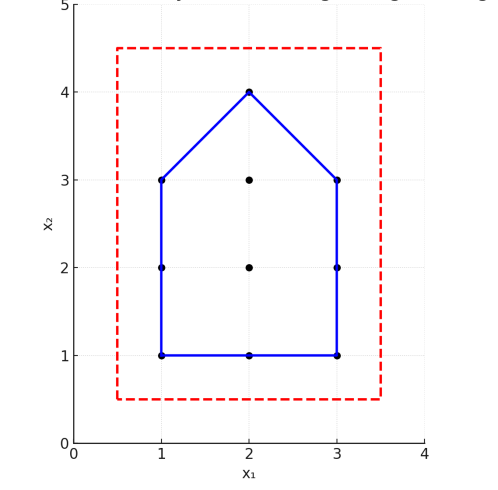
Figure 1: MIO relaxations. Black dots represent the discrete feasible region of an MIO problem. Blue lines depict the convex hull, while dashed red lines depict a weaker linear relaxation.

and $h$ are convex, then the problem is referred as a convex mixed-integer nonlinear optimization (convex MINLO). Finally, when $g$ and $h$ are general nonlinear functions, the problem is called simply mixed-integer nonlinear optimization (MINLO) (Belotti et al. 2013, Floudas 1995, Lazimy 1982, Vielma 2015, Wolsey and Nemhauser 1999). These classes of problems are nested, e.g., MILOs are special cases of MIQOs which in turn are special cases of MICOs, and so forth. As a simple rule of thumb, MILOs are generally significantly easier to solve than the other classes with current technology, and general MINLO are substantially more difficult than convex MINLOs.

Optimization problem (3) is non-convex and may be hard to solve due to presence of integrality constraints $\mathbf{z}\in\mathbb{Z}^{p}$, while its natural continuous relaxation obtained by dropping these constraints is easier to handle. In particular, for convex MINLOs, the continuous relaxation is typically easy to solve to optimality since any local minimum is a global minimum. MIO problems with strong continuous relaxations, that is, with continuous relaxations that are close approximations of the discrete problems, can often be solved to optimality at medium or large scales. The best possible convex relaxation of an MIO, which we refer to as the convex hull relaxation, ensures that it can be solved as a convex problem, see Figure 1 for a depiction. MIO problems with weak relaxations, on the other hand, cannot be solved to optimality without substantial enumeration, which may be prohibitive computationally at large scales. In fact, strength of the continuous relaxation is often a better predictor of the difficulty of an MIO problem than more natural metrics such as number of variables or constraints.

MIOs have become a powerful tool for ML in recent years, thanks to their modeling capabilities and advancements in solving techniques. For instance, we can model ML tasks as MIOs by letting the decision variables $\mathbf{z}$ and $\mathbf{r}$ correspond to model parameters $\boldsymbol{\theta}$, the constraints of (3) define the space of $f_{\boldsymbol{\theta}}$, and the objective function of (3) calculate the loss function $\ell$. Unlike traditional methods for learning ML models, the objective function and constraints can be more easily customized to address various model desiderata and domain-specific constraints. Furthermore, MIOs can be modeled in and solved with a number of solvers to optimality or with guarantees on solution quality. Moreover, state-of-the-art MIO solvers are equipped with powerful general purpose heuristics, and can typically find high-quality solutions to optimization problems in seconds.

1.5 Structure of this Tutorial

This tutorial will explore recent advances on using MIOs for responsible ML. Section 2 examines MIO-based methods for developing interpretable ML models and for explaining black-box models to enhance transparency. We then discuss robustness to the issues of data availability, quality, and bias in Section 3. Section 4 is devoted to policy learning problems and in section 5, we examine how MIO can be used to enforce some important principles in ML, particularly fairness. We conclude the tutorial with section 6, where we highlight unresolved and/or underexplored issues in responsible ML that MIO has the potential to address, paving the way for future research on this topic.

2 Interpretability and Explainability

Model transparency in ML can be achieved through two strategies: building inherently transparent models or generating explanations for black-box models. Interpretable machine learning refers to learning white-box models such that the learned ML model is “comprehensible” for humans. Such white-box models may correspond to simple classes of $f_{\boldsymbol{\theta}}$ (e.g., additive rules), functions that can be expressed using pencil and paper, sequential logical statements, and/or visualizations that enhance understanding (Rudin et al. 2022). One method of quantifying interpretability is proposed by Jo et al. (2023), which they call decision complexity. The decision complexity of a classifier is the minimum number of parameters needed to make a prediction on a new datapoint. This definition captures interpretability through the concepts of simpler, human-comprehensible model classes and sparsity constraints. A critical consideration when using an interpretable model is a potential interpretability-accuracy trade-off, where accuracy may decrease as the models considered become more interpretable (Alcalá et al. 2006, Baryannis et al. 2019, Dziugaite et al. 2020, Johansson et al. 2011, You et al. 2022). The magnitude of such a trade-off and the benefits of gaining model interpretability under some loss in accuracy is domain-specific.

Explainable artificial intelligence (XAI), on the other hand, refers to methods used to explain black-box models for human comprehension. Explanations can use texts, visuals, examples, relevant features, or a comparable interpretable model, and can be localized to a subspace of the data or globally applied. The major challenge is learning explanations that are simple, are precise, and have large coverage (Li et al. 2022, Ribeiro et al. 2018). Note that in high-stakes domains, interpretable models are preferred over explanations if the learning task, dataset, and domain allow for it and the tradeoff in accuracy is low (Rudin 2019). XAI methods, on the other hand, can preserve the power of any ML model while providing some transparency.

MIOs have recently emerged as a natural modeling and solution tool for interpretable ML, as they are able to model logical constraints, integrality restrictions, and sparsity inherent in such models. Sections 2.1 and 2.2 explore how MIO has been used for interpretable supervised learning for additive and logical models, respectively. We also explore MIOs for unsupervised learning tasks such as principal component analysis (PCA), network learning and clustering in section 2.3. In section 2.4, we show how MIOs have been used to help explain the outputs of black-box models via counterfactual explanations.

2.1 Additive Models for Supervised Learning

In this section, we explore how MIO can be used to learn (generalized) linear ML models. Specifically, $f_{\boldsymbol{\theta}}$ is defined as a linear function, that is,

$$f_{\boldsymbol{\theta}}(\mathbf{x})=\boldsymbol{\theta}^{\top}\mathbf{x}.$$ (4)

The function $f_{\boldsymbol{\theta}}$ can be used for regression tasks where $f_{\boldsymbol{\theta}}$ maps to a predicted label (linear regression) or a predicted probability (logistic regression and risk scoring), or used in binary classification by thresholding the predicted value of $f_{\boldsymbol{\theta}}$ by 0. To enhance interpretability, $\boldsymbol{\theta}$ can be restricted to be integer-valued and/or sparse. We explore four additive methods in this section: linear regression (section 2.1.1), logistic regression and risk scores (section 2.1.2), support vector machines (section 2.1.3), and generalized additive models (section 2.1.4).

2.1.1 Subset Selection and Sparse Linear Regression

Given a covariate $\mathbf{x}$, linear regression predicts a response via the learned relation $f_{\boldsymbol{\theta}}(\mathbf{x})=\boldsymbol{\theta}^{\top}\mathbf{x}$. The function $f_{\boldsymbol{\theta}}(\mathbf{x})$ is found by solving problem (2) using the least squares loss $\ell(f_{\boldsymbol{\theta}}(\mathbf{x}^{i}),y^{i})=(y^{i}-\boldsymbol{\theta}^{\top}\mathbf{x}^{i})^{2}$, a method called ordinary least squares (OLS). If the number of features $d$ is small, OLS solutions are interpretable, as the sign and magnitude of a coefficient associated with each feature serves as a simple proxy of the effect of that feature. However, interpretability quickly fades if $d$ is large. Consider for example the “Communities and crime” dataset, containing socio-economic data, law enforcement data and crime data (US census, LEMAS survey and FBI) from $n=1,993$ cities and involving $d=100$ features. Figure 2a depicts the OLS solution: while effective at explaining the data, with a large $R^{2}$ value, the output is hard to interpret or use by policy makers.

To add interpretability to a linear regression model, penalties or constraints that limit the number of non-zero elements (sparsity) of $\boldsymbol{\theta}$ can be added. Traditional approaches in the statistical literature add an L1 penalty (Tibshirani 1996) $\lambda_{1}\|\boldsymbol{\theta}\|_{1}$ (a method called lasso), or a combination of an L1 and L2 penalties (Zou and Hastie 2005) $\lambda_{1}\|\boldsymbol{\theta}\|_{1}+\lambda_{2}\|\boldsymbol{\theta}\|_{2}^{2}$ (referred to as elastic net), where the regularization parameters $\lambda_{1},\lambda_{2}\in\mathbb{R}_{+}$ need to be tuned. Indeed, if $\lambda_{1}$ is large enough, optimal solutions are sparse and interpretable. Figure 2b shows the lasso solution where parameter $\lambda_{1}$ is tuned to produce four nonzero elements: while the solution is indeed interpretable, the low $R^{2}$ value suggests that the estimator fails to accurately explain the data. The poor accuracy occurs since the L1 penalty is an approximation of the sparsity of $\boldsymbol{\theta}$, but does not models it explicitly. A more accurate representation involves the so-called L0 norm, defined as $\|\boldsymbol{\theta}\|_{0}=\sum_{j=1}^{d}\text{1}[\theta_{j}\neq 0]$ for 1 the indicator function. Note that the L0 penalty is not actually a norm as it violates homogeneity, and (unlike norms) is non-convex. As a consequence, optimization problems involving such terms may be difficult to solve. The least squares problem with L0 and L2 regularization is

$$\min_{\boldsymbol{\theta}\in\mathbb{R}^{d}}\ \sum_{i\in\mathcal{I}}(y^{i}-\boldsymbol{\theta}^{\top}\mathbf{x}^{i})^{2}+\lambda_{0}\|\boldsymbol{\theta}\|_{0}+\lambda_{2}\|\boldsymbol{\theta}\|_{2}^{2},$$ (5)

where $\lambda_{0},\lambda_{2}\in\mathbb{R}_{+}$ are hyperparameters to be tuned. If $\lambda_{2}=0$ and the L0 norm is enforced as a constraint instead of a penalty, problem (5) is the best subset selection problem (Miller 1984). Figure 2c depicts the solution of problem (5), which is both interpretable and accurate.

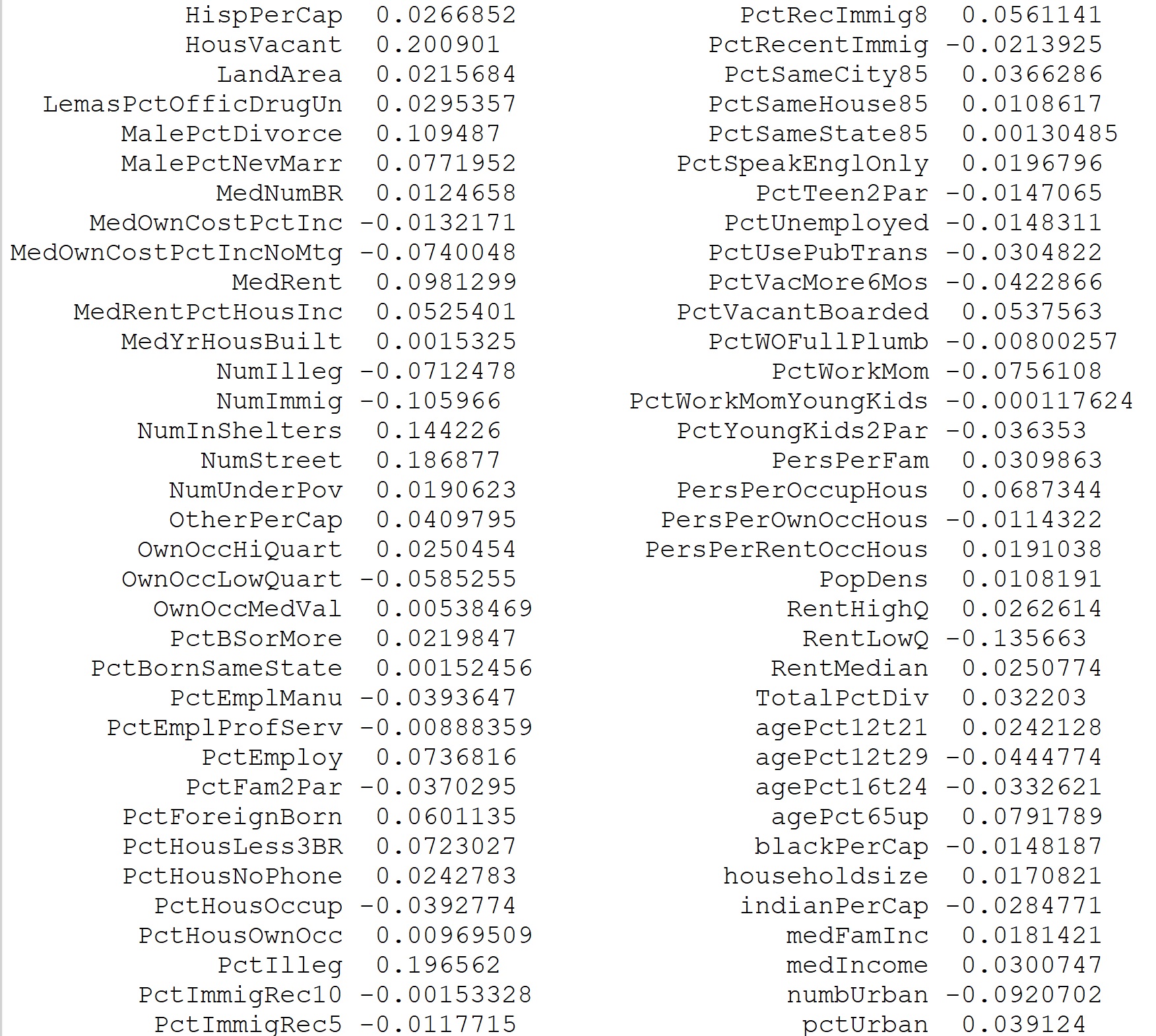
(a) OLS, $R^{2}=0.84$

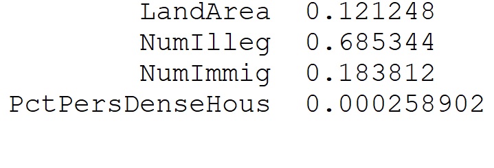
(b) Lasso, $R^{2}=0.25$

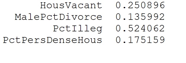
(c) Problem (5), $R^{2}=0.81$

Figure 2: Solutions from three linear regression methods. The ordinary least squares (a) produces a solution that is not interpretable. The lasso estimator (b) can be used to produce interpretable solutions, but the low $R^{2}$ value calls in question the accuracy. Using MIO (c), an accurate and interpretable solution is found. LandArea: land area in square miles, NumIlleg: number of kids born to never married, NumImmig: total number of people known to be foreign born, PctPersDenseHous: percent of persons in dense housing (more than 1 person per room), HousVacant: number of vacant households, MalePctDivorce: percentage of males who are divorced.

There has been tremendous progress in solving (5) using MIO technology over the past decade. Earlier works (Bertsimas et al. 2016, Gómez and Prokopyev 2021, Wilson and Sahinidis 2017, Miyashiro and Takano 2015b, a) were based on reformulating the L0 constraint using big-M constraints. Letting $\mathbf{z}\in\{0,1\}^{d}$ be binary variables used to encode the support of $\boldsymbol{\theta}$, problem (5) can be reformulated as

$$\min \sum_{i\in\mathcal{I}}(y^{i}-\boldsymbol{\theta}^{\top}\mathbf{x}^{i})^{2}+\lambda_{0}\sum_{j=1}^{d}z_{j}+\lambda_{2}\sum_{j=1}^{d}\theta_{j}^{2}$$ (6)

s.t. $$-Mz_{j}\leq\theta_{j}\leq Mz_{j} \forall j\in[d]$$

$$\boldsymbol{\theta}\in\mathbb{R}^{d},\mathbf{z}\in\{0,1\}^{d},$$

where the value of constant $M$ is typically chosen heuristically. As pointed out in (Dong et al. 2015), optimal solutions of the continuous relaxation of (6) satisfy $z_{j}^{*}=|\theta_{j}|/M$, thus the continuous relaxation reduces to penalizing the L1 norm of the regression coefficients, i.e., the popular lasso estimator (Tibshirani 1996). Using the natural formulation (6) led to the possibility of solving to optimality problems with $d$ in the dozens or low hundreds (Bertsimas et al. 2016) – a notable improvement over alternative exact methods available at the time, but insufficient in several practical applications.

A major breakthrough in tackling (6) was achieved by using the perspective reformulation (Xie and Deng 2020, Dong et al. 2015, Bertsimas and Van Parys 2020, Atamturk and Gomez 2020), an MIO convexification technique originally derived using disjunctive programming (Aktürk et al. 2009, Ceria and Soares 1999, Frangioni and Gentile 2006, Günlük and Linderoth 2010). At a high level, the reformulation first introduces additional epigraphical variables $r_{j}\geq\theta_{j}^{2}$, moving the nonlinearities induced by the ridge regularization to the constraints. Then it multiplies the left-hand side of the new constraints by $z_{j}$, resulting in formulation

$$\min_{\boldsymbol{\theta}\in\mathbb{R}^{d},\mathbf{z}\in\{0,1\}^{d}}\ \sum_{i\in\mathcal{I}}(y^{i}-\boldsymbol{\theta}^{\top}\mathbf{x}^{i})^{2}+\lambda_{0}\sum_{j=1}^{d}z_{j}+\lambda_{2}\sum_{j=1}^{d}r_{j}$$ (7a)

s.t. $$\theta_{j}^{2}\leq z_{j}r_{j} \forall j\in[d]$$ (7b)

$$-Mz_{j}\leq\theta_{j}\leq Mz_{j} \forall j\in[d].$$ (7c)

Since $0\leq z_{j}\leq 1$ in any feasible solution of the continuous relaxation, constraints (7b) produce a tighter relaxation than simple big-M formulations – in fact, the big-M constraints can be safely removed. Moreover, since $\theta_{j}^{2}\leq z_{j}r_{j}\Leftrightarrow\sqrt{(2\theta_{j})^{2}+(z_{j}-r_{j})^{2}}\leq z_{j}+r_{j}$ (an identity that can be easily verified by squaring both sides of the inequality), and since function $h(\theta,z,r)=\sqrt{(2\theta)^{2}+(z-r)^{2}}-z+r$ is convex (since it is the sum of an L2 norm and a linear function), problem (7) is an MICO. Constraints (7b), referred to as rotated cone constraints, can in fact modeled directly as is in most MICO solvers, with the software automatically performing the aforementioned transformation automatically. In fact, since 2022, the MIO solver Gurobi automatically performs this reformulation even when presented with the weaker formulation (6). The use of the perspective reformulation (7) increased the dimension of problems that can be solved by an order-of-magnitude, with researchers reporting solutions to problems with $d$ in the hundreds to low thousands.

A second major breakthrough was achieved by Hazimeh et al. (2022): instead of relying on general purpose solvers, they implemented a branch-and-bound algorithm tailored for sparse regression based on formulation (7). Critically, they rely on first-order coordinate descent methods to solve the continuous relaxations, which scale to large-dimensional problems much better than the interior point methods or outer approximations used by most off-the-shelf solvers. The authors report optimal solutions to problems with $d$ in the hundreds of thousands to millions.

The progress in solving (5) to optimality illustrates the potential of MIO technology: in just a decade, the scale of problems that could be solved to optimality increased by several orders-of-magnitude, from dozens to hundreds of thousands. Some of the limitations of current methods is the dependence on the ridge term $\lambda_{2}\|\boldsymbol{\theta}\|_{2}^{2}$ to strengthen the formulation, as well as tailored branch-and-bound methods depending on the absence of additional constraints on the regression variables. Naturally, there is ongoing research addressing these limitations (Atamturk and Gomez 2025, Tillmann et al. 2024). In addition, there is also additional effort in developing primal methods to find high-quality solutions quickly as well as to better understand the statistical merits of solving (5) to optimality (Hazimeh and Mazumder 2020, Mazumder et al. 2023).

2.1.2 Logistic Regression and Risk Scores

In logistic regression, the aim is to learn the probabilities that a given covariate $\mathbf{x}$ has some binary class label $y\in\{-1,1\}$.

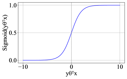
Figure 3: The sigmoid function $\sigma(y\boldsymbol{\theta}^{\top}\mathbf{x})=\frac{1}{1+\exp(-y\boldsymbol{\theta}^{\top}\mathbf{x})}$, whose value represents the estimated probability that an individual with covariates $\mathbf{x}$ has label $y$. The logistic loss is $-\log(\sigma(y\boldsymbol{\theta}^{\top}\mathbf{x}))$.

Namely, we learn a linear model $\boldsymbol{\theta}^{\top}\mathbf{x}$ where a larger value indicates a higher probability that the true label of $\mathbf{x}$ is $y=1$. The loss function for logistic regression is the logistic loss, also called the cross-entropy loss, which involves the sigmoid function and takes the form $\ell(f_{\boldsymbol{\theta}}(\mathbf{x}^{i}),y^{i})=\log(1+\exp(-y^{i}(\boldsymbol{\theta}^{\top}\mathbf{x}^{i})).$ We refer to Figure 3 for an explanation of the logistic loss. Similarly to OLS, logistic regression is considered relatively interpretable provided that the number of features $d$ is sufficiently small (Hosmer and Lemeshow 2000).

Similarly to least squares regression, an $\lambda_{0}$ penalty $\lambda_{0}\|\boldsymbol{\theta}\|_{0}$ can be added to logistic regression to encourage sparsity by selecting only a few non-zero coefficients. However, while the logistic loss is convex, it is also significantly harder to handle than quadratic losses in the context of branch-and-bound algorithms, limiting the effectiveness of MIO methods. Sato et al. (2016) present an MILO formulation which uses a piecewise linear convex approximation of the logistic loss in conjunction with big-M constraints to model the L0 sparsity penalty (as described in section 2.1.1). If a separable regularization term is present in the objective function of the logistic regression, then perspective methods similar to those reported in section 2.1.1 can be used, e.g., see (Deza and Atamtürk 2022). Alternatively, researchers have recently started to consider other relaxations for sparse logistic regression involving more sophisticated convexification techniques (Shafiee and Kılınç-Karzan 2024). Nonetheless, effort towards solving sparse logistic regression is relatively recent and current MIO technology is less mature than methods for solving least square regression problems (5). To date, researchers have reported the ability to solve problems with $d$ in the hundreds. Naturally, further improvements may be achieved in a near future, but for now the best approaches in high-dimensional settings may be primal methods that do not guarantee optimality (Dedieu et al. 2021).

Sparse logistic regression can also be used as a basis for learning risk scores, see Figure 4 for an example. A risk score is defined by a small set of questions with integral answers (in the example, answers are binary corresponding to yes/no questions); a decision-maker can then quickly add all the answers to obtain a score representing a prediction or risk of a patient. Traditionally, risk scores were designed by human experts, but there has been recent work in learning risk scores optimally from data. Indeed, a risk scoring scheme can be learned by solving the following problem using the logistic loss:

$$\min \sum_{i\in\mathcal{I}}\left[\log(1+\exp(-y^{i}(\boldsymbol{\theta}^{\top}\mathbf{x}^{i}))\right]+\lambda_{0}\sum_{j=1}^{d}z_{j}$$ (8)

s.t. $$lz_{j}\leq\theta_{j}\leq uz_{j} \forall j\in[d]$$

$$\boldsymbol{\theta}\in\mathbb{Z}^{d},\mathbf{z}\in\{0,1\}^{d}$$

where $l$ and $u$ are lower and upper bounds on the potential answers. The two main differences between sparse logistic regression and risk scores learning are: (a) variables $\boldsymbol{\theta}$ are restricted to be integer, as the addition of integer numbers by hand is substantially easier than adding rational or real numbers; (b) variables $\boldsymbol{\theta}$ are bounded, as addition of small integer numbers is easier than large ones.

Figure 4: A possible scoring card to assess medical risk. See Ustun and Rudin (2019) for samples of optimal risk scoring cards in a variety of high-stakes domains.

Ustun and Rudin (2019) use MILO-based approaches to solve (8), constructing outer approximations of the logistic loss – note that the approach differs from Sato et al. (2016) in the sense that the linear outer approximation is dynamically constructed within the branch-and-bound tree, instead of being defined a priori. The authors report solutions to problem with $d$ in the dozens – sufficient to tackle several problems in high-stakes domains, but this approach would not scale to large-dimensional problems. We point out that since the release of that paper, several general-purpose off-the-shelf solvers support branch-and-bound algorithms with exponential cones, and can directly tackle (8) without requiring tailored implementations of outer approximations. Molero-R´ıo and D’Ambrosio (2024) generalize the approach to continuous data $\{\mathbf{x}^{i}\}_{i\in\mathcal{I}}$, although this generalization results in much more difficult problems: exact solutions were obtained by the authors in instances with $d\leq 5$, and heuristics are proposed for larger dimensions.

2.1.3 Support Vector Machines

Given data with possible labels $\mathcal{Y}=\{-1,1\}$, support vector machines (SVMs) are classification models that use a separating hyperplane $f_{\boldsymbol{\theta}}(\mathbf{x})$ of the form (4) to divide the space of covariates $\mathbf{x}$ into two, with each section corresponding to a possible label, see Figure 5. Requiring that points with different labels are on different sides of the hyperplane can be encoded via constraints $\boldsymbol{\theta}^{\top}\mathbf{x}^{i}>0$ for all points such that $y^{i}=1$, and $\boldsymbol{\theta}^{\top}\mathbf{x}^{i}<0$ for all points such that $y_{i}=-1$ – or, concisely, as $y_{i}\cdot\boldsymbol{\theta}^{\top}\mathbf{x}^{i}\geq\epsilon$ for all $i\in\mathcal{I}$, where $\epsilon$ can be interpreted as a small number used to represent the strict inequality. However, multiple hyperplanes may separate the data equally well, and SVMs call for the one that is farthest from the data. Mathematically, this can be accomplished by choosing $\epsilon$ to be as large as possible while keeping the norm of $\boldsymbol{\theta}$ constant (as indeed, any vector of the form $c\boldsymbol{\theta}$ with $c\in\mathbb{R}$ represents the same hyperplane), or ensuring that $\boldsymbol{\theta}$ is of minimum norm while keeping $\epsilon$ constaint, e.g., $\epsilon=1$. Since data is rarely separable in practice, a hinge penalty of the form $\max\{0,\epsilon-y_{i}\cdot\boldsymbol{\theta}^{\top}\mathbf{x}^{i}\}$ is added, which has value $0$ for correctly classified points but penalizes misclassifications proportionally to their distance to the hyperplane. Finally, similarly to previous subsections, a sparsity penalty can be added to enforce interpretability, resulting in the optimization problem (Dedieu et al. 2021)

$$\min\ \frac{1}{2}\|\boldsymbol{\theta}\|_{2}^{2}+\lambda_{1}\sum_{i\in\mathcal{I}}r_{i}+\lambda_{0}\sum_{j=1}^{d}z_{j}$$ (9a)

s.t. $$y^{i}\left(\boldsymbol{\theta}^{\top}\mathbf{x}^{i}\right)\geq 1-r_{i} \forall i\in\mathcal{I}$$ (9b)

$$-Mz_{j}\leq\theta_{j}\leq Mz_{j} \forall j\in[d]$$ (9c)

$$\boldsymbol{\theta}\in\mathbb{R}^{d},\boldsymbol{z}\in\{0,1\}^{d},\mathbf{r}\in\mathbb{R}_{+}^{n},$$ (9d)

where $\lambda_{1}$ and $\lambda_{0}$ are hyperparameters to be tuned and $r_{i}$ represents the value of the hinge penalty for datapoint $i\in\mathcal{I}$.

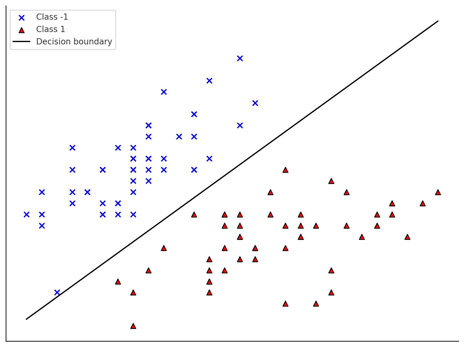
Figure 5: A SVM classifier on perfectly separable data.

Interestingly, while SVMs are among to most widely used models in statistics and ML, there are surprisingly limited results in the literature concerning solving their interpretable version (9) to optimality. The methods proposed by Dedieu et al. (2021) focus mostly on first order methods that deliver high-quality solutions quickly, but no proof of optimality. The authors also showcase the performance of exact methods in some synthetic instances, but it is unclear how the results would extend to real data. Guan et al. (2009) propose to use perspective relaxations (similar to those discussed in section 2.1.1) but report numerical issues when using off-the-shelf solvers – note however that solvers have improved substantially in the 15 years since the publication of that paper. Lee et al. (2022) propose branch-and-bound algorithms for a related SVM problem with group sparsity, and they report solutions to problems with $d\approx 60$.

2.1.4 Generalized Additive Models

Generalized additive models (GAMs) broaden the definition of $f_{\boldsymbol{\theta}}(\mathbf{x})$ given in (4), allowing the elements of $\mathbf{x}$ to be transformed by potentially nonlinear functions. For example, given a predefined class of one-dimensional functions $f_{k}:\mathbb{R}\to\mathbb{R}$ indexed by set $\mathcal{K}$, we can write the GAM

$$f_{\boldsymbol{\theta}}(\mathbf{x})=\sum_{j=1}^{d}\sum_{k\in\mathcal{K}}\theta_{jk}f_{k}(x_{j}),$$ (10)

where $\boldsymbol{\theta}$ are the parameters to be estimated. Unlike the previous additive models, GAMs are useful for capturing more complex and nonlinear relationships while still preserving a simpler structure for interpretability. Navarro-García et al. (2025) consider sparse least squares problems where functions $f$ are given by splines, and Cozad et al. (2014) use elementary functions compatible with the solver Baron for a downstream decision-making task. Another usual form of GAM is obtained by adding pairwise interactions of the form

$$f_{\boldsymbol{\theta}}(\mathbf{x})=\sum_{j=1}^{d}\sum_{l=1}^{d}\theta_{ij}x_{i}x_{j},$$ (11)

see (Ibrahim et al. 2024, Wei et al. 2022) for methods in the context of sparse least squares problems. While exisiting approaches have been mostly proposed for least squares regression problems, the approaches in sections 2.1.2 and 2.1.3 can also be naturally extended to account for GAMs.

2.2 Logical Models for Supervised Learning

In this section, we explore how MIO is useful for creating optimal and interpretable logical models. Logical models use “if-then,” “or,” and “and” relationships between statements to define $f_{\boldsymbol{\theta}}(\mathbf{x})$. Thus, they can be easily be described via text and/or visuals, making them inherently transparent. Unlike linear models, logical models can capture non-linear relationships and naturally work well with categorical and multiclass datasets (Rudin et al. 2022). Typically, MIO-based logical models minimize the 0-1 loss $\ell(f_{\boldsymbol{\theta}}(\mathbf{x}^{i}),y^{i})=\text{1}[f_{\boldsymbol{\theta}}(\mathbf{x}^{i})\neq y^{i}]$, which directly maximizes the training accuracy. These models often include some sparsity penalty that limits the number of statements that define $f_{\boldsymbol{\theta}}$. In this section, we discuss three types of logical models: decision trees in section 2.2.1, and rule lists and decision sets in section 2.2.2.

2.2.1 Decision Trees

Decision trees are a popular interpretable logical model due to its ease of visualization, and are used widely in applications. A classification tree is a model which takes the form of a binary tree. At each branching node, a test is performed, which directs a sample to one of its descendants. Thus, each data sample, based on its features, follows a path from the root of the tree to a leaf node, where a label is predicted. Because learning decision trees that optimize training accuracy is $NP$-hard, there exist many heuristic approaches that locally optimize other metrics like Gini impurity or information gain (Breiman et al. 2017).

Bertsimas and Dunn (2017) provide one of the first MILO formulations for optimal classification trees, where the tree is constrained by a pre-specified depth $D$ and big-M constraints are used to specify the routing of datapoints in the tree. Following this work, there has since been a growing body of work to improve on such a formulation to improve computational tractability. For example, Verwer and Zhang (2017, 2019) propose to reduce the number of variables and constraints of Bertsimas and Dunn (2017) in order to explore the branch-and-bound tree faster, albeit at the cost of weakening the continuous relaxation. Alternatively, Aghaei et al. (2024) and Günlük et al. (2021) propose stronger formulations for settings with binary or categorical data, without increasing the size of the MIO formulations.

We now discuss the approach of Aghaei et al. (2024), which uses a flow-based formulation.

Figure 6: A visualization of the flow network used to train a decision tree of depth $D=2$ in Aghaei et al. (2024).

We visualize the notation and flow network used in Figure 6, and provide details of the formulation in the following. Consider a binary tree of maximum depth $D$ where each node is indexed using breadth-first search from 1 to $2^{D}-1$. We let $\mathcal{B}:=\{1,\ldots,2^{D-1}-1\}$ contain the indexes of all internal nodes and $\mathcal{L}:=\{2^{D-1},\ldots,2^{D}-1\}$ be the indexes of all leaf nodes. For node $k\in\mathcal{B}$, we denote the left child as $l(k):=2k$, the right child as $r(k):=2k+1$, and the parent node as $a(k)$. Assuming that the covariates are binarized in the training data (i.e., $\mathbf{x}^{i}\in\{0,1\}^{d}$ for all $i\in\mathcal{I}$), let $\theta_{k,j}\in\{0,1\}$ be the decision variable that equals $1$ if and only if at node $k\in\mathcal{B}$, feature $j\in[d]$ is tested on. Then if $x^{i}_{j}=0$ where $b_{k,j}=1$, datapoint $i$ flows to $l(k)$, and otherwise is routed to $r(k)$. We let decision variable $\phi_{k,y}\in\{0,1\}$ equal 1 if and only if node $k$ predicts label $y$.

We now create a flow network that will be used to formulate the MILO for learning optimal classification trees. We introduce source node $s$ and sink node $t$, where we add an edge from $s$ to $1$ as an entry point into the network and an edge from every node $k\in\mathcal{B\cup L}$ to the sink $t$. We introduce binary decision variables $z^{i}_{a(k),k}\in\{0,1\}$ for every data point $i\in\mathcal{I}$ and $k\in\mathcal{B\cup L}$ that equals 1 if and only if the $i$th datapoint is correctly classified in the tree and traverses the edge from $a(k)$ to $k$. We also define flow variables to the sink $z^{i}_{k,t}\in\{0,1\}$ for all $k\in\mathcal{L}$ and $i\in\mathcal{I}$ that equals 1 if and only if $\phi_{k,y^{i}}=1$ and $i$ visits node $k$ (i.e., $i$ is correctly classified at node $k$). We can minimize the 0-1 misclassification loss by maximizing the number of correct classifications, where $i$ is correctly classified if and only if $\sum_{k\in\mathcal{B\cup L}}z^{i}_{k,t}=1$. We then have the following formulation to learn an optimal classification tree:

$$\max\ \sum_{i\in\mathcal{I}}\sum_{k\in\mathcal{B\cup L}}z^{i}_{k,t}$$ (12a)

s.t. $$\sum_{j=1}^{d}\theta_{k,j}=1 \forall k\in\mathcal{B}$$ (12b)

$$\sum_{y\in\mathcal{Y}}\phi_{k,y}=1 \forall k\in\mathcal{L}$$ (12c)

$$z^{i}_{a(k),k}=z^{i}_{k,l(k)}+z^{i}_{k,r(k)} \forall k\in\mathcal{B}$$ (12d)

$$z^{i}_{a(k),k}=z^{i}_{k,t} \forall k\in\mathcal{L}$$ (12e)

$$z^{i}_{k,l(k)}\leq\sum_{j\in[d]:x^{i}_{j}=0}\theta_{k,j} \forall k\in\mathcal{B}$$ (12f)

$$z^{i}_{k,r(k)}\leq\sum_{j\in[d]:x^{i}_{j}=1}\theta_{k,j} \forall k\in\mathcal{B}$$ (12g)

$$z^{i}_{k,t}\leq\phi_{k,y^{i}} \forall k\in\mathcal{L}$$ (12h)

$$\theta_{k,j}\in\{0,1\} \forall k\in\mathcal{B},j\in[d]$$ (12i)

$$\phi_{k,y}\in\{0,1\} \forall k\in\mathcal{L},y\in\mathcal{Y}$$ (12j)

$$z^{i}_{a(k),k}\in\{0,1\} \forall i\in\mathcal{I},k\in\mathcal{B\cup L}$$ (12k)

$$z^{i}_{k,t}\in\{0,1\} \forall i\in\mathcal{I},k\in\mathcal{L}$$ (12l)

Constraints (12b) and (12c) ensure that only one feature is tested on at each node in $\mathcal{B}$ and one label is predicted at each leaf in $\mathcal{L}$, respectively. We specify flow conservation constraints in (12d) and (12e). Constraints (12f) and (12g) ensure that datapoint $\mathbf{x}^{i}$ gets routed through the tree correctly based on the set of tests $\theta_{k,j}$. We also restrict $z^{i}_{k,t}$ to be 0 if leaf $k$ does not predict the correct label for datapoint $i$ in constraint (12h). Since then, there have been several extensions and improvements over the aformentioned works (Alès et al. 2024, Hua et al. 2022, Liu et al. 2024, D’Onofrio et al. 2024, Zhu et al. 2020, Elmachtoub et al. 2020). We refer to the review paper of Carrizosa et al. (2021) for further discussion on MILO for decision trees.

2.2.2 Rule Lists and Decision Sets

Rule lists (also called decision lists) and decision sets are logical models that are often expressed with text. Rule lists in particular use “if-then-else” statements in succession. At each statement, if $\mathbf{x}$ satisfies a conjunction of statements, then a prediction is made, else the next statement is tested (or another prediction is made if at the last statement). Rule lists can be expressed as a special case of binary decision trees, where each node that a test is performed has at least one child that predicts a class. We provide an example of rule lists in Figure 7a. Rudin and Ertekin (2018) formulate an MILO for creating falling rule lists, which is a rule list with monotonically decreasing probabilities of the positive class in each successive “then”. They encode rule lists through a set of binary decision variables: variables to denote which “if-then” statements are selected, variables to denote the ordering of selected statements, and variables to track rule list predictions on the training datapoints. Using some of the bounds introduced in Rudin and Ertekin (2018), Angelino et al. (2018) improve on solve times with a branch-and-bound algorithm for learning optimal rules lists for categorical data.

Decision sets are statements in disjunctive normal form, i.e., if one from a set of “and” statements are satisfied, then one label is assigned; otherwise, another label is assigned. Decision sets differ from decision trees and rule lists in that they are unordered and not hierarchical, expressible as a collection of “if-else” statements rather than nested statements. We provide an example of a decision set in Figure 7b. Similar to the encoding of rule lists, decision sets can be expressed as a set of binary decision variables that indicate which conjunctions are used and what prediction is made for each training datapoint. With such an encoding, Wang and Rudin (2015) introduce an MILO for learning decision sets that minimize the number of misclassifications, inducing sparsity by penalizing the number of features used in each conjunction and the number of conjunctions used.

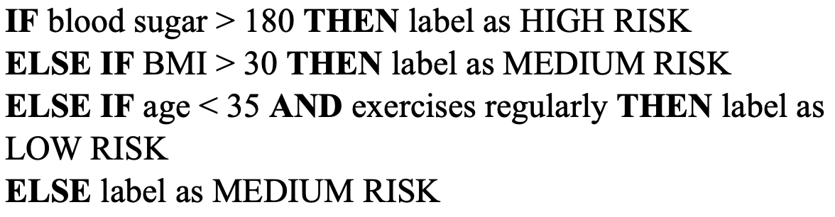
(a) Rule List

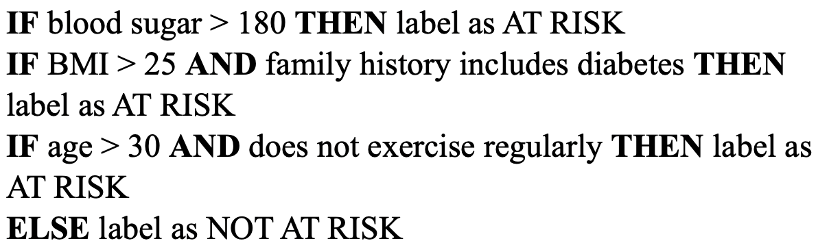
(b) Decision Set

Figure 7: A rule list and decision set example on predicting diabetes risk.

2.3 Interpretable and Explainable Unsupervised Learning

We will now explore some transparent models for unsupervised learning tasks of the form (1). In particular, we explore interpretable dimensionality reduction, graph learning and clustering techniques. Dimensionality reduction methods learn a mapping $f_{\boldsymbol{\theta}}(\mathbf{x}):\mathbb{R}^{d}\mapsto\mathbb{R}^{d^{\prime}}$ for $d^{\prime}<d$, which can be used to map $\mathbf{x}$ to a lower dimensional space while maintaining as much information as possible. Graph learning seeks to represent the joint distribution of a set of variables as a graph encoding conditional independence assumptions. Clustering refers to methods that group values of $\mathbf{x}^{i}$ in the data together based on some metric, learning a mapping $f_{\boldsymbol{\theta}}(\mathbf{x})$ from the data to an assigned cluster. We discuss MILO-based methods for dimensionality reduction (specifically, principal component analysis) in section 2.3.1, inference of Bayesian networks in section 2.3.2, and clustering in section 2.3.3.

2.3.1 Sparse Principal Component Analysis

Principal component analysis (PCA) is a classical technique for dimensionality reduction in unsupervised learning. At a high level, PCA seeks the most important axes or directions, called principal components, that explain the variation in the data. In particular, the first principal component $\boldsymbol{\theta}\in\mathbb{R}^{d}$ is the vector such that $f_{\boldsymbol{\theta}}(\boldsymbol{x})=\boldsymbol{\theta^{\top}x}$ has the largest variance, which can be used for example to create a linear rule that serves to best differentiate the population. Consider the example shown in Figure 8: if the data is projected into its first principal component (oriented up and right), an accurate summary of the data can be obtained requiring only one value instead of two.

Mathematically, the first $k$ principal components correspond to the eigenvectors of $\mathbf{X^{\top}X}$ (sample covariance matrix of the training data) associated with the $k$ largest eigenvalues, where the matrix of training samples $\mathbf{X}\in\mathbb{R}^{n\times d}$ is assumed to be centered. While they can be computed easily, the principal components are typically dense and often not interpretable. Similarly to the methods discussed in section 2.1, interpretability can be enforced by requiring the components to be sparse via an L0 constraint. Formally, the problem of finding the first sparse principal component can be formulated as the MINLO

$$\max_{\boldsymbol{\theta}\in\mathbb{R}^{d}}\ \frac{1}{n}\mathbf{\boldsymbol{\theta}^{\top}\mathbf{X^{\top}X}\boldsymbol{\theta}}$$ (13a)

s.t. $$\|\boldsymbol{\theta}\|_{2}^{2}\leq 1$$ (13b)

$$-z_{j}\leq\theta_{j}\leq z_{j} \forall j\in[d]$$ (13c)

$$\sum_{j=1}^{d}z_{j}\leq\delta$$ (13d)

$$\mathbf{z}\in\{0,1\}^{d},\boldsymbol{\theta}\in\mathbb{R}^{d}.$$ (13e)

Note that if the big-M constraint (13c) is removed, essentially making the discrete variables redundant since $\boldsymbol{z}=\boldsymbol{0}$ is optimal, then (13) reduces to a well-known characterization of the largest eigenvalue of matrix $\mathbf{X^{\top}X}$. In other words, (13) seeks a sparse approximation of the maximum eigenvalue.

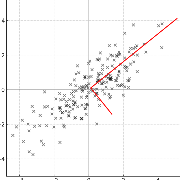
Figure 8: 2D datasets and principal components, where lengths represent the amount of variance captured.

The continuous relaxation of problem (13) is non-convex, as the objective corresponds to the maximization of a convex function. While several general purpose MINLO solvers now accept problems with non-convex quadratic relaxations, such a direct approach is currently not particularly effective. Instead, note that for any given $\mathbf{z}\in\{0,1\}^{d}$, problem (13) reduces to a thrust region problem (that is, optimization of a quadratic function subject to a ball constraint), a class problems where the standard Shor semidefinite optimization (SDO) relaxation is exact. The Shor relaxation linearizes the objective by introducing a matrix variable $\boldsymbol{T}$ such that $T_{ij}=\theta_{i}\theta_{j}$; in matrix form, we can write $\boldsymbol{T}=\boldsymbol{\theta\theta^{\top}}$. With the introduction of this matrix variable, the objective $\sum_{i=1}^{d}\sum_{j=1}^{d}(\boldsymbol{X^{\top}X})_{ij}T_{ij}$ is linear in $\boldsymbol{T}$, and all non-convexities are subsumed into the equality constraint $\boldsymbol{T}-\boldsymbol{\theta\theta^{\top}}=\boldsymbol{0}$. The equality constraint is then relaxed as $\boldsymbol{T}-\boldsymbol{\theta\theta^{\top}}\in\mathcal{S}_{+}^{d}\Leftrightarrow\begin{pmatrix}1&\boldsymbol{\theta^{\top}}\\ \boldsymbol{\theta}&\boldsymbol{T}\end{pmatrix}\in\mathcal{S}_{+}^{d+1}$, where $\mathcal{S}_{+}^{d+1}$ denotes the cone of positive semidefinite matrices.

In a celebrated paper, d’Aspremont et al. (2004) present a SDO approximation of (13), where the original variables $\boldsymbol{\theta}$ are projected out and additional constraints on the matrix variable $\boldsymbol{T}$ are imposed. Li and Xie (2024) and Kim et al. (2022) further improve on this relaxation using MIO techniques, resulting in continuous relaxations with optimality gaps inferior to 1% in practice. In a similar vein,  Moghaddam et al. (2005) and Berk and Bertsimas (2019) propose algorithms for solving (13) to optimality using branch-and-bound. Nonetheless, solving SDO problems is itself a challenging task, let alone mixed-integer SDOs: exact methods scale to problems with $d$ in the low hundreds. Therefore, there have also been approaches that approximate sparse PCA problems using MIO methods (Dey et al. 2022, Wang and Dey 2020).

2.3.2 Bayesian Networks

Bayesian networks are critical tools in the field of causal inference and knowledge discovery. They aim to describe the joint probability distribution generating the data by means of a directed acyclic graph (DAG) $\mathcal{G}=(\mathcal{V},\mathcal{A})$. The vertex set $\mathcal{V}=[d]$ corresponds to the features in the data, while each arc $(j,k)\in\mathcal{A}$ encodes conditional independence relations in the data: specifically, each node is conditionally independent of its non-descendants given its parents. Figure 9 depicts a simple Bayesian network: if the status of a disease is known, the symptoms experienced by the patient and test results are independent, while being clearly correlated if the patient is not aware of whether they have a disease or not.

Learning a Bayesian network can be formulated as an MIO. For all ordered pairs of features $(j,k)$, define a decision variables $z_{jk}$ to indicate whether $(j,k)\in\mathcal{A}$ ($z_{jk}=1$) or not ($z_{jk}=0$), and consider the optimization problem

$$\min_{\boldsymbol{\theta}\in\Theta,\;\mathbf{z}\in\{0,1\}^{d\times d}}\ \sum_{k\in\mathcal{V}}\sum_{i\in\mathcal{I}}\ell(f_{\boldsymbol{\theta},k}(\mathbf{x}^{i}\circ\mathbf{z}_{\cdot k}),x_{k}^{i})+g(\boldsymbol{\theta},\mathbf{z})$$ (14a)

s.t. $$z_{kk}=0\quad \forall k\in\mathcal{V}$$ (14b)

$$\text{The graph $\mathcal{G}$ induced by $\mathbf{z}$ is acyclic},$$ (14c)

where $\mathbf{z}_{\cdot k}\in\{0,1\}^{d}$ is the vector collecting all elements with second coordinate $k$, i.e., $(\mathbf{z}_{\cdot k})_{j}=z_{jk}$, and ‘$\circ$’ refers to the Hadamard or entrywise product of vectors, so that $\mathbf{x}^{i}\circ\mathbf{z}_{\cdot k}$ can be interpreted as the subvector of $\mathbf{x}^{i}$ induced by the nonzero elements of $\mathbf{z}_{\cdot k}$. The loss function $\ell(f_{\boldsymbol{\theta},k}(\mathbf{x}^{i}\circ\mathbf{z}_{\cdot k}),x_{k}^{i})$ indicates the prediction error of estimating $x_{k}^{i}$ using the other entries indicated by $\mathbf{z}$ with model $f_{\boldsymbol{\theta},k}$. Function $g$ is a function promoting regularization, for example $g(\boldsymbol{\theta},\mathbf{z})=\sum_{j\in\mathcal{V}}\sum_{k\in\mathcal{V}}z_{jk}$ to ensure the graph is sparse and interpretable. Constraints (14b) ensures that no feature is used to estimate its own value, and constraints (14c), which require an explicit mathematical formulation, ensure no cycles in the graph. Essentially, problem (14) attempts to design an acyclic graph such that the estimation of each feature based on the value of its parents is as accurate as possible. Note that if constraints (14c) are removed, then (14) reduces to $d$ independent versions of (2) (potentially with additional sparsity constraints), but the acyclic constraints result in non-trivial couplings of these problems.

Figure 9: Bayesian network

Two challenges need to be overcome to solve (14). The first challenge is to find a tractable representation of the nonlinear and potential non-convex objective. Jaakkola et al. (2010) considers the simplest case where functions $f_{\boldsymbol{\theta}}$ are separable, while several authors have considered more sophisticated cases where $f_{\boldsymbol{\theta}}$ are linear functions (Manzour et al. 2021, Küçükyavuz et al. 2023, Park and Klabjan 2017). The second challenge is handling the combinatorial constraints (14c). A first approach is to use similar cycle breaking constraint as those arising in linear optimization formulations for spanning trees (Magnanti and Wolsey 1995) or MIO formulations for traveling salesman and vehicle routing problems (Laporte and Nobert 1987):

$$\sum_{j\in S}\sum_{k\in S}z_{jk}\leq|S|-1\qquad\forall S\subseteq\mathcal{V}.$$ (15)

Indeed, observe that cycles defined by nodes $S\subseteq\mathcal{V}$ involve exactly $|S|$ arcs: inequalities (15) thus prevent such cycles from happening. Constraints (15) typically result in strong relaxations, but the exponential number of constraints poses an algorithmic hurdle. In MILO settings, formulations with exponentially many constraints can typically be handled effectively (Bartlett and Cussens 2017). Unfortunately, if modeling the loss functions requires nonlinear terms, then the technology is less mature and algorithms based on formulation (15) are not effective. Currently, a better approach is to introduce additional integer variables $\zeta_{j}\in\{1,\dots,d\}$ that can be interpreted as the position they appear in a topological ordering of the DAG. Then (14c) can be reformulated as

$$1-d(1-z_{jk})\leq\zeta_{k}-\zeta_{j}\quad\forall j,k\in V,$$

which can be interpreted as follows: if $z_{jk}=0$ then the constraint is redundant, but if $z_{jk}=1$ then node $k$ is forced to have a later position than $j$ in the order. This alternative reformulation results in a substantially weaker relaxation, but requires only a quadratic number of constraints, resulting in relaxations that are easier to handle. Using these constraints, Manzour et al. (2021) and Küçükyavuz et al. (2023) propose to tackle (14) for the case of least squares loss as

$$\min\ \sum_{k\in\mathcal{V}}\sum_{i\in\mathcal{I}}\left(x_{k}^{i}-\sum_{j\in\mathcal{V}}\theta_{jk}x_{j}^{i}\right)^{2}+\sum_{j\in V}\sum_{k\in V}z_{jk}$$ (16a)

s.t. $$\theta_{jj}=0\quad \forall j\in V$$ (16b)

$$-Mz_{jk}\leq\theta_{jk}\leq Mz_{kj}\quad \forall i,j\in V$$ (16c)

$$1-d(1-z_{jk})\leq\zeta_{k}-\zeta_{j}\quad \forall j,k\in V$$ (16d)

$$\boldsymbol{\theta}\in\mathbb{R}^{d\times d},\;\mathbf{z}\in\{0,1\}^{d\times d},\;\boldsymbol{\zeta}\in\{0,1\}^{d},$$ (16e)

where they also use perspective reformulations as described in section 2.1.1. Observe that if $z_{jk}=0$, then constraints (16c) ensure that $\theta_{jk}=0$ and therefore feature $j$ is not used in model that predicts feature $k$. Naturally, problem (16) is harder to solve than (7) as it requires to estimate substantially more parameters, introduces many more variables and difficult constraints: the authors report solutions to problems with up to $d=100$ features, allowing for uses in some high-stakes domains such as healthcare. Other approaches that have used MIO to learn Bayesian Networks are Chen et al. (2021) and Eberhardt et al. (2024).

2.3.3 Interpretable clustering

A clustering of a dataset $\{\mathbf{x}^{i}\}_{i\in\mathcal{I}}$ is a partition $\mathcal{C}_{1}\cup\mathcal{C}_{2}\cup\dots\cup\mathcal{C}_{m}=\mathcal{I}$, such that individuals assigned to the same group $\mathcal{C}_{k}$ are presumed to be similar, and dissimilar to individuals assigned to different clusters. Popular clustering methods in the ML literature such as K-means are not easily interpretable, as they do not provide a clear argument of why a given datapoint belongs to a given cluster. Recent works have proposed interpretable clustering methods by noting that logical methods for supervised learning, as described in section 2.2, produce a partition of the data, e.g., the leaves of a decision tree.

Carrizosa et al. (2023) propose to modify formulations such as (12) to design interpretable clustering methods as follows. Given a dissimilarity metric $d_{ij}$ between datapoints $i,j\in\mathcal{I}$, e.g., $d_{ij}=\|\mathbf{x}^{i}-\mathbf{x}^{j}\|$ for some given norm, and letting $z_{i}^{k}\in\{0,1\}$ be a binary variable that indicates datapoint $i$ is assigned to partition $k$, they use the objective function

$$\min\sum_{i\in\mathcal{I}}\sum_{j\in\mathcal{I}}\sum_{k\in\mathcal{B}\cup\mathcal{L}}d_{ij}z_{k}^{i}z_{k}^{j}.$$ (17)

For example, in the context of decision trees, partitions correspond to leaves and variables $z_{k}^{i}$ in (17) correspond to variables $z_{a(k),k}^{i}$ with $k\in\mathcal{L}$ in (12). Note that Carrizosa et al. (2023) use logic rules instead of decision trees, but we adapt their approach to decision trees for notational simplicity. If two points are assigned to the same partition, then there is a penalty of $d_{ij}$ in the objective (17), while no penalty is incurred if assigned to different partitions.

The objective function (17) is nonlinear and non-convex as it involves products of binary variables. Nonetheless, there is a vast amount of literature associated with handling this class of functions – we describe two of the most popular methods next. The first approach uses McCormick linearizations (McCormick 1976): introduce additional variables $\zeta_{k}^{ij}$ representing the products $z_{k}^{i}z_{k}^{j}$, and add the linear constraints

$$0\leq\zeta_{k}^{ij},\;-1+z_{k}^{i}+z_{k}^{k}\leq\zeta_{k}^{ij},\;\zeta_{k}^{ij}\leq z_{k}^{i},\;\zeta_{k}^{ij}\leq z_{k}^{j}.$$ (18)

Observe that for any $z_{k}^{i},z_{k}^{j}\in\{0,1\}$, the only feasible solution to the McCormick system is indeed setting $\zeta_{k}^{ij}=z_{k}^{i}z_{k}^{j}$. Linearization (18) is indeed the proposed approach in Carrizosa et al. (2023). The second approach (Poljak and Wolkowicz 1995) convexifies the nonlinear objective function as

$$\min\sum_{i\in\mathcal{I}}\sum_{j\in\mathcal{I}}\sum_{k\in\mathcal{B}\cup\mathcal{L}}d_{ij}z_{k}^{i}z_{k}^{j}+\lambda\sum_{i\in\mathcal{I}}\sum_{k\in\mathcal{B}\cup\mathcal{L}}\left(\left(z_{k}^{i}\right)^{2}-z_{k}^{i}\right)$$ (19)

with $\lambda>0$. Since for any $z_{k}^{i}\in\{0,1\}$ the identity $\left(z_{k}^{i}\right)^{2}=z_{k}^{i}$ holds and (19) coincides with (17) for integer solutions. However, the strength of the continuous relaxation degrades as $\lambda$ increases, since for any $0<z_{k,t}^{i}<1$ the inequality $\left(z_{k}^{i}\right)^{2}<z_{k}^{i}$ holds. Nonetheless, if $\lambda$ is sufficiently large, then (19) is a convex quadratic function that can be handled effectively by MIQO solvers. Neither of these approaches is in general better than the other, since both degrade the relaxation quality (but in different ways), and while (18) requires introducing additional variables and constraints, (19) introduces additional nonlinearities. Fortunately, commercial MIO solvers accept (17) directly as an input and decide automatically which reformulation to use.

Other approaches to design interpretable clusters based on more sophisticated metrics have been considered in the literature (Bertsimas et al. 2021, Lawless et al. 2022). They consider using the Silhouette metric (Rousseeuw 1987), defined as ratios involving the intracluster distances and distances to the second nearest cluster. However, this metric is highly non-convex, and the authors have thus resorted to heuristic approaches instead of exact methods.

2.4 Counterfactual Explanations

Counterfactual explanations (CEs) are a method of explaining black-box ML models through a statement like “if this datapoint changed to this value, then this outcome would have been predicted instead” (Lewis 2013). CEs are useful for explaining decisions that come from black box models, and provide actionables for individuals in the data on how to change their data to get a different outcome. For instance, a CE for some point $\bar{\mathbf{x}}$ that received a class label $\bar{y}$ may be to find a $\mathbf{x}$ close to $\bar{\mathbf{x}}$ that received a desired class label $y$. Mathematically, let some cost metric $c(\cdot,\cdot):\mathbb{R}^{d}\times\mathbb{R}^{d}\mapsto\mathbb{R}$ encode information on how feasible it is to change $\bar{\mathbf{x}}$ into $\mathbf{x}$, where a larger value indicates a less feasible change. For black-box model $f_{\boldsymbol{\theta}}(\mathbf{x})$ that assigns a class label, we want to solve

$$\min_{\mathbf{x}} c(\mathbf{x},\bar{\mathbf{x}})$$ (20)

s.t. $$f_{\boldsymbol{\theta}}(\mathbf{x})=y.$$

The complexity of this problem depends on the metric $c$ used, the encoding of $f_{\boldsymbol{\theta}}$ in the constraints, and additional domain requirements, e.g., constraints on which and how many features can change in practice. Cui et al. (2015) and Parmentier and Vidal (2021) use an MILO formulation to learn a counterfactual explanation for ensemble tree methods. Kanamori et al. (2020, 2021) propose MILO-based methods for (20) that get CEs close to the empirical distribution of the data and account for interactions among features. Mohammadi et al. (2021) provide CEs for neural network models using MILO, providing optimality and coverage guarantees in using their method. Counterfactual explanations are not just useful for black-box models, but can also be useful for interpretable models. Ustun et al. (2019) and Russell (2019) develop an MILO-based framework for counterfactual explanations in interpretable classification tasks like logistic regression, SVMs, and linearized rule lists and decision sets. Carreira-Perpiñán and Hada (2021) learn CEs for multivariate decision trees, formulating the problem as an MIO and solving the integer variables by enumerating over tree leaves.

There are several recent works that extend beyond problem (20), and are able to generate multiple CEs at once. Carrizosa et al. (2024a, b) present MIQO formulations for learning CEs in score-based classifications (e.g., logistic regression and SVMs) in two settings: learning collective CEs across multiple individuals to help detect patterns and insights in CEs and learning CEs with functional data. Maragno et al. (2024) can also create robust CEs that are robust to small perturbations of the data, yielding a region of CEs instead of just one CE through robust optimization methods (see section 3 on robustness) and MIO. We refer to Guidotti (2024) for more information on recent advancements in learning counterfactual explanations.

3 Robustness

Real-world datasets are often imperfect and deployment conditions can differ from training conditions. A robust ML model maintains reliable performance despite such discrepancies. In such settings, MIOs can preserve interpretability and sparsity while training a robust model, and effectively handle challenges with discrete datasets. We explore how MIO can help train or verify models that are robust to three common data issues: outliers, adversarial attacks, and distribution shifts. Outliers are anomalous observations not generated by the same process as the bulk of data, and can distort models if not handled. Adversarial attacks are deliberate, small perturbations to inputs designed to mislead the model. Distribution shifts are changes in the distribution of the data between training and deployment (e.g., due to evolving data collection or population drift). This section discusses each of these challenges in turn and how to model and solve them with MIO.

3.1 Outlier detection

Outliers can adversely affect model accuracy on the majority of data because many learning algorithms (like least squares) give every point equal influence in the objective. To make linear models more robust to outliers, one approach is to limit or down-weight the influence of outlier points during training. A classical robust regression method is least trimmed squares (LTS), which fits an ordinary least squares regression while ignoring a certain fraction of the most extreme residuals (Rousseeuw 1984, Rousseeuw and Leroy 2003). In other words, LTS attempts to find model parameters $\boldsymbol{\theta}$ that minimize the error on all but the worst $k$ data points (trimming off $k$ outliers).

An optimization problem that simultaneously flags datapoints as outliers and fits a model with the rest of the training data can be formulated as an MIO by introducing binary variables to select which data points to exclude from the fit. Letting $z_{i}\in\{0,1\}$ indicate whether data point $i$ is discarded as an outlier ($z_{i}=1$) or included in the fit ($z_{i}=0$), an MINLO formulation is

$$\min_{\boldsymbol{\theta}\in\mathbb{R}^{d},\mathbf{z}\in\{0,1\}^{n}} \sum_{i\in\mathcal{I}}\ell(f_{\boldsymbol{\theta}}(\mathbf{x}^{i}),y^{i})(1-z_{i})$$ (21)

s.t. $$\sum_{i\in\mathcal{I}}z_{i}\leq k,$$

where $k\in\mathbb{Z}_{+}$ is the maximum number of outliers allowed. The continuous relaxation of (21) is highly nonlinear and non-convex due to the products of binary variables with the nonlinear loss function: in the case of the least trimmed squares where $\ell$ is quadratic loss, the optimization problem is cubic and difficult to solve exactly (Giloni and Padberg 2002). More recent approaches attempt a reformulation with a simpler continuous relaxation: for example, consider

$$\min_{\boldsymbol{\theta}\in\mathcal{R}^{d},\mathbf{z}\in\{0,1\}^{n},\boldsymbol{r}\in\mathbb{R}^{d}}\; \ell(f_{\boldsymbol{\theta}}(\mathbf{x}^{i}),y^{i}-r_{i})$$ (22a)

s.t. $$-Mz_{i}\leq r_{i}\leq Mz_{i}$$ (22b)

$$\sum_{i\in\mathcal{I}}z_{i}\leq k.$$ (22c)

Intuitively, $\mathbf{r}$ can be interpreted as a vector of “corrections” to the label $\mathbf{y}$. If $z_{i}=0$, then constraints (22b) ensure $r_{i}=0$ and there is no correction to the data; if $z_{i}=1$, then $r_{i}$ is arbitrary and in optimal solutions $r_{i}=y_{i}-f_{\boldsymbol{\theta}}(\mathbf{x}^{i})$, i.e., the correction is such that the label matches exactly the prediction from model $f_{\boldsymbol{\theta}}$, incurring a zero loss (thus effectively discarding the point). Formulation (22) was proposed by Insolia et al. (2022) in the context of the LTS problem, see also Zioutas and Avramidis (2005) and Zioutas et al. (2009) for alternative formulations. The key advantage of (22) is that its continuous relaxation is of the same class as the nominal problem, and is convex if (2) is. Unfortunately, the continuous relaxation is also extremely weak: if constraints $\mathbf{z}\in\{0,1\}^{\mathcal{I}}$ are relaxed, then setting $z_{i}=\epsilon$ for all $i\in\mathcal{I}$, $\boldsymbol{\theta}$ to any arbitrary value (e.g., such that $f_{\boldsymbol{\theta}}(\mathbf{x})=0$ is the constant function) and $r_{i}=y_{i}-f_{\boldsymbol{\theta}}(\mathbf{x})$ is optimal with a trivial objective value of $0$. As a consequence, formulation (22) struggles with problems with $n$ in the hundreds, even when the loss is quadratic.

Nonetheless, new innovations are being proposed in the literature. For example, Gómez and Neto (2023) propose improved relaxations similar to those presented in §2.1.1, although the implementation is more complex. Moreover, several works consider special cases arising in inference of graphical models, where the additional structure can be leveraged to construct simpler relaxations or even design polynomial-time algorithms (Bhathena et al. 2025, Han and Gómez 2024, Gómez 2021). Moreover, while most of the work cited focuses on LTS problems or similar variants, recent approaches consider logistic regression (Insolia et al. 2021), least median of squares problems (Bertsimas and Mazumder 2014, Puerto and Torrejón 2024) or support vector machine problems with outliers (Cepeda et al. 2024). While the specific implementations may differ for other ML models, the methods share similar difficulties and potential.

3.2 Adversarial Attacks and Verification

Adversarial attacks refer to small, intentionally crafted perturbations of input data that cause an ML model $f_{\boldsymbol{\theta}}$ to misclassify the input. Formally, given an instance $\mathbf{x}$ with true (or initially predicted) label $y=f_{\boldsymbol{\theta}}(x)$, an adversarial attack finds a perturbation $\mathbf{u}$ that is small in terms of a prespecified norm and radius, ($\|\mathbf{u}\|\leq\epsilon$), but that results in a different label assignment ($y\neq f_{\boldsymbol{\theta}}(\mathbf{x}+\mathbf{u})$). Robustness to adversarial attacks means that no such perturbation exists. Verifying a model’s robustness can be posed as a constrained optimization:

$$\min_{\mathbf{u}\in\mathbb{R}^{d}} \|\mathbf{u}\|$$ (23)

s.t. $$f_{\boldsymbol{\theta}}(\mathbf{x}+\mathbf{u})=k,$$

where $k\neq y$ is given a priori; if the objective value of (23) is greater than $\epsilon$, then the ML model can be certified as robust for the specific input $\mathbf{x}$ and label $k$. In practice, determining that a given ML model is truly robust requires solving (23) a plethora of times for different possible inputs, which can be done in parallel if enough computational resources are available. Note that in this case the ML model is trained a priori, thus the parameters $\boldsymbol{\theta}$ are given and not decision variables.

If function $f_{\boldsymbol{\theta}}$ is simple, e.g., affine in the input, then problem (23) is easy and may be even solvable by inspection. However, if the ML model is complex, then the nonlinear equality constraint in problem (23) may pose substantial difficulties. In such cases, MIO provides a framework to exactly search for adversarial examples and certify robustness, especially for models with discrete or piecewise-linear structure. For instance, for a ReLU-based neural network, the non-convexities required to model $f_{\boldsymbol{\theta}}$ correspond to the activation functions (Tjeng et al. 2017). Indeed, modeling the output of a trained artificial neural network involves handling non-convex equality constraints of the form

$$\max\{0,\boldsymbol{\theta}^{\top}\mathbf{r}\}=s,$$ (24)

where $\boldsymbol{\theta}$ are given weights, $\mathbf{r}$ are decision variables representing the pre-activation variables at a given neuron (i.e., outputs from the previous layer), and $s$ is a decision variable representing the post-activation variable or output of the neuron. If lower bounds and upper bounds such that $l\leq\boldsymbol{\theta}^{\top}\mathbf{r}\leq u$ are known, non-convex constraints such as (24) can be linearized using the system

$$0\leq s,\;\boldsymbol{\theta}^{\top}\mathbf{r}\leq s,\;s\leq uz,\;s\leq\boldsymbol{\theta}^{\top}\mathbf{r}-l(1-z),$$

where $z\in\{0,1\}$ is an auxiliary binary variable representing the logical condition $z=\text{1}[\boldsymbol{\theta}^{\top}\mathbf{r}\geq 0]$.

Tjeng et al. (2017) pioneered this MIO verification approach for piecewise-linear networks. The continuous relaxations can be weak, and thus direct MIO approaches do not scale to practical sizes. However, in a series of works by Anderson et al. (2020b, a) and Tjandraatmadja et al. (2020), it is shown how to further improve the relaxation using MIO methods. The resulting formulation can either be used directly to verify small networks, or used as a basis for a propagation heuristic that scales to large datasets while improving the performance versus competing alternatives. Note that while solving these MIOs can be computationally intensive, they offer strong guarantees: any solution found is a genuine adversarial example, and if none is found, the model is provably robust (under the defined attack model). This is in contrast to heuristic attacks or incomplete verification methods which might miss worst-case attacks. See also Aftabi et al. (2025), Patil and Mintz (2022), Thorbjarnarson and Yorke-Smith (2021, 2023), Khalil et al. (2018), Venzke and Chatzivasileiadis (2020), and Hojny et al. (2024) for related work on MIO methods for handling robustness with artificial neural networks. MIO based methods have also been proposed to verify tree ensembles (Kim et al. 2022, Kantchelian et al. 2016, Zhang et al. 2020).

3.3 Robustness to Adversarial Attacks and to Distribution Shifts

Rather than only verifying robustness post hoc, we can use MIO at training time to build models that account for distribution shifts or adversarial attacks. A natural approach to enhance robustness is to integrate adversarial perturbation scenarios during training, e.g., by adding attacks detected with methods described in section 3.2 as new instances in the training set. Such methods treat both the algorithms describing the learning model and the attack pattern as black boxes and can be used in a variety of contexts, but may be inefficient in practice as they require retraining the model and detecting attacks several times.

An alternative approach is to use robust optimization (which prepares the model to handle malicious or extreme perturbations to features) or distributionally robust optimization (which ensures good performance for all test distributions in some sense “close” to the training distribution) paradigms. Robust optimization methods require describing an uncertainty set $\mathcal{U}\subseteq\mathbb{R}^{n\times d}$, corresponding to all possible attacks, and tackles the robust counterpart of the nominal training problem (2) defined as

$$\min_{\boldsymbol{\theta}\in\Theta}\;\;\max_{\mathbf{U}\in\mathcal{U}}\hskip 5.69054pt\sum_{i\in\mathcal{I}}\ell(f_{\boldsymbol{\theta}}(\mathbf{x}^{i}+\mathbf{u}^{i}),y^{i}),$$ (25)

where $\mathbf{u}^{i}$ denotes the $i$-th row of $\mathbf{U}$ and corresponds to the attack/shift on datapoint $i\in\mathcal{I}$. Distributionally robust optimization formulations yield optimization problems similar in structure to (25). Robust and distributionally robust approaches have been widely used in machine learning, see for example Kuhn et al. (2019). A vast majority of approaches operate under convexity or continuity assumptions, in which case (25) can be conveniently handled by reformulating it as an equivalent deterministic optimization problem using duality arguments. However, duality methods cannot be directly applied in the presence of non-convexities. For example the loss function may not be non-convex, corresponding to a discrete $0-1$ loss or a piecewise linear classifier such as a decision tree or artificial neural network (Kurtz and Bah 2021, Vos and Verwer 2022). Alternatively, the uncertainty set $U$ may be discrete, e.g., when modeling perturbations to integer or categorical features (Sun et al. 2025, Belbasi et al. 2023), or a combination of both sources of non-convexities (Justin et al. 2021, 2023). MIO technology can be effective in settings when duality fails.

A common approach to tackle robust optimization problems under non-convexities is to use delayed constraint generation methods. Problem (25) can be reformulated with the introduction of an epigraphical variable as

$$\min_{\boldsymbol{\theta},r}\; r$$ (26a)

s.t. $$\sum_{i\in\mathcal{I}}\ell(f_{\boldsymbol{\theta}}(\mathbf{x}^{i}+\mathbf{u}^{i}),y^{i})\leq r\qquad\forall\mathbf{U}\in\mathcal{U},$$ (26b)

transforming the $\min$-$\max$ optimization problem into a deterministic problem with a large (potentially infinite) number of constraints. Delayed constraint generation methods alternate between: (a) “processing” relaxations of problem (26) where set $\mathcal{U}$ is replaced with a finite subset containing candidate attacks/shifts, obtaining promising solutions $(\bar{\boldsymbol{\theta}},\bar{r})$; (b) solving the separation problem

$$\min_{\mathbf{U}\in\mathcal{U}}\;\bar{r}-\sum_{i\in\mathcal{I}}\ell(f_{\bar{\boldsymbol{\theta}}}(\mathbf{x}^{i}+\mathbf{u}^{i}),y^{i})$$ (27)

to detect the most damaging attack/shift to the solution $(\bar{\boldsymbol{\theta}},\bar{r})$, and adding it to the set of candidate attacks. Note that a naive implementation of constraint generation methods, where “processing” corresponds to “solving to optimality,” reduces to the iterative procedure described in the first paragraph of the subsection. However, better implementations based on MIO algorithms, e.g., by adding inequalities as a subroutine while constructing a single branch-and-bound tree, can achieve orders-of-magnitude improvements in computational times. Even better methods are possible when the non-convex separation problem (27) can be reformulated (or accurately approximated) as a convex optimization problem. For example, in the setting considered by Sun et al. (2025), problem (27) can be solved via dynamic programming, a method that solves combinatorial problems by breaking them down into simpler subproblems and solves each subproblem only once while avoiding redundant computations. They then exploit the fact that a dynamic programming scheme can be encoded as a shortest path problem on a DAG, and use linear optimization duality to recover an exact deterministic formulation of polynomial size. This deterministic reformulation is shown to perform an order-of-magnitude better than constraint generation approaches.

4 Observational Settings

Causal inference aims to learn the effects of a treatment on an outcome, focusing on cause-and-effect relationships rather than just correlations (Hernán and Robins 2010). In such settings, we have covariates, represented by random variable $X$ with $d$ features, that are assigned treatments, represent by variable $A$. After a treatment $A$ is given to $X$, an outcome is observed, represented by random variable $Y(A)$. If we want to observe the effect of a treatment on the outcome, we would want $A\mathrel{\perp\!\!\!\perp}X$, meaning that each $X$ is assigned a treatment $A$ randomly. The random assignment of treatments among individuals in an experiment is called a randomized control trial (RCT). In an RCT, the effects of treatment $A$ can be directly observed in the outcome without bias from each individual’s covariates.

However, conducting RCTs present practical and ethical issues in many domains. For example, in healthcare settings, it may not be ethical to withhold medical treatment at random, or there may be existing policies that dictate the assignment of treatments in the population. In such settings, observational data may be collected instead, where data is collected via an external, unobserved policy. Observational data introduces selection bias as treatments are not assigned randomly, making it difficult to measure the effect of the treatment variable without other observed and unobserved confounding factors.

The datasets we consider are of the form $\{\mathbf{x}^{i},a^{i},y^{i}\}_{i\in\mathcal{I}}$ for $\mathbf{x}^{i}\in\mathbb{R}^{d}$, the covariates, $a^{i}$ the historical treatment from a set of treatments $\mathcal{A}$, and an observed outcome $y^{i}\in\mathcal{R}$. Note that in such a dataset, the response $y^{i}$ is only observed under treatment $a^{i}$, and we do not have the counterfactual outcomes under any other treatment in $\mathcal{A}$. One primary goal in such settings is thus to estimate counterfactual outcomes, which help measure such treatment effects.

In causal inference, a requirement to generate meaningful counterfactual outcomes is to assume strong ignorability (Rosenbaum and Rubin 1983), which we define as follows:

Assumption 1 (Strong Ignorability)

The treatment assignment $A$ is independent of the potential outcomes $Y(a)$ for all $a\in\mathcal{A}$ conditional on the covariates $X$. That is, for all $a\in\mathcal{A}$, $Y(a)\mathrel{\perp\!\!\!\perp}A\mid X$. Furthermore, the probability of receiving any treatment given X must be positive. That is, $\mathbb{P}(A=a\mid X=\mathbf{x})>0$ for all $a\in\mathcal{A}$ and $\mathbf{x}\in\mathbb{R}^{d}$.

The first condition in Assumption 1 is called ignorability or conditional exchangeability, whereas the second condition is called positivity. Note that although strong ignorability is a common and often necessary assumption in causal inference, it is challenging to verify in practice with observational data. Lastly, we also assume consistency, which states that the potential outcome predicted is equal to the observed outcome in the data. That is, for $Y$ the observed outcome, $Y=Y(A)$. We will assume strong ignorability and consistency throughout this section.

With these standard causal inference assumptions in mind, we explore two streams that use causal inference and MIO together in observational settings. Section 4.1 details matching methods to estimate counterfactual outcomes, and section 4.2 explores learning prescriptive policies in observational settings.

4.1 Matching to Estimate Counterfactual Outcomes

One method to estimate counterfactual outcomes is via matching. For example, given a treatment group and a control group, where the control group is presumed to be larger, the idea is to match each individual from the treatment group with one or several individuals from the control group with similar characteristics, as illustrated in Figure 10. Then, counterfactual estimates for individuals in the treatment group, corresponding to outcomes if no intervention is performed, can be obtained by averaging the observed outcomes for matched individuals in the treatment group.

$$\min_{\mathbf{z}\in\{0,1\}^{\mathcal{T}\times\mathcal{C}}}\; \sum_{t\in\mathcal{T}}\sum_{c\in\mathcal{C}}d_{tc}z_{tc}$$ (28a)

s.t. $$\sum_{c\in\mathcal{C}}z_{tc}=m \forall t\in\mathcal{T}$$ (28b)

$$\sum_{t\in\mathcal{T}}z_{tc}\leq 1 \forall c\in\mathcal{C}$$ (28c)

Figure 10: Matching in observation studies

Consider the following optimization problem to match between a treatment and a control group ($|\mathcal{A}|=2$), where $\mathcal{T}\subseteq\mathcal{I}$ are the individuals that received a treatment and $\mathcal{C}=\mathcal{I}\setminus\mathcal{T}$ denotes the control group, where we assume that $m|\mathcal{T}|\leq|\mathcal{C}|$ for some $m\in\mathbb{Z}_{+}$. Letting $d_{tc}$ be a metric of the dissimilarity between $t\in\mathcal{T}$ and $c\in\mathcal{C}$, e.g., $d_{tc}=\|\mathbf{x}^{t}-\mathbf{x}^{c}\|$, consider the optimization problem where decision variables $z_{tc}=1$ if and only if individuals $t$ and $c$ are matched together. Constraint (28b) ensures that each individual in the treatment group is matched with $m$ individuals of the control group, constraint (28c) ensures that no individual in the treatment group is paired with two or more treated individuals, and the objective seeks matches with small dissimilarities.

Optimization problem (28) is easy to solve and does not require sophisticated MIO technology. In fact, the feasible region of the continuous relaxation has a special property: every extreme point of the polytope induced by constraints (28b)-(28c) and constraints $\mathbf{0}\leq\mathbf{z}\leq\mathbf{1}$ is integral. Thus, since the objective function is linear, there exists an optimal solution of the linear optimization relaxation that is an extreme point and thus satisfies the integrality restrictions. Recognizing polytopes with integral extreme points is in general hard, but some special cases can be recognized immediately. In the case of (28), imagine that both sides of constraints (28b) are multiplied by $-1$. Then observe that all variables appear in at most two constraints (not including bound constraints) with opposite signs: any constraint matrix satisfying this condition is totally unimodular, and the resulting polytope is guaranteed to have integral extreme points.

While formulation (28) is attractive due to its computational simplicity, the resulting matching could be low-quality and lead to poor counterfactual estimations. Indeed, while the overall dissimilarity is minimized, it is possible that the subset of the control population used differs substantially from the treated individuals in the values of some critical features. Mathematically, given a covariate $j$,

$$\frac{1}{|\mathcal{T}|}\sum_{t\in\mathcal{T}}x_{j}^{t}\not\approx\frac{1}{m|\mathcal{T}|}\sum_{t\in\mathcal{T}}\sum_{c\in\mathcal{C}}x_{j}^{c}z_{tc},$$

where the left hand size is the average value of covariate $j$ in the treatment group, and the right hand size represents that average value for the selected individuals in the control group. Naturally, if feature $j$ is critical to the outcomes under no treatment, then any counterfactual estimation based on formulation (28) would be poor.

Traditionally, this covariate imbalance has been tackled through heuristic iterative procedures. However, Zubizarreta (2012) proposed to instead modify the objective of (28) to

$$\min_{\mathbf{z}\in\{0,1\}^{\mathcal{T}\times\mathcal{C}}}\;\sum_{t\in\mathcal{T}}\sum_{c\in\mathcal{C}}d_{tc}z_{tc}+\sum_{j\in[d]}\lambda_{j}\left|\frac{1}{m|\mathcal{T}|}\sum_{t\in\mathcal{T}}\sum_{c\in\mathcal{C}}x_{j}^{c}z_{tc}-\frac{1}{|\mathcal{T}|}\sum_{t\in\mathcal{T}}x_{j}^{t}\right|,$$

where $\lambda_{j}$ are weights representing the importance of each covariate, to ensure balanced covariates. This modification destroys the integrality property of the MIO formulation: while the feasible region has not changed, the objective is now nonlinear and optimal solutions of the continuous relaxation may no longer be extreme points. The MILO reformulation of the ensuing optimization problem given by

$$\min_{\mathbf{z}\in\{0,1\}^{\mathcal{T}\times\mathcal{C}},\mathbf{r}\in\mathbb{R}^{d}}\; \sum_{t\in\mathcal{T}}\sum_{c\in\mathcal{C}}d_{tc}z_{tc}+\sum_{j\in[d]}\lambda_{j}r_{j}$$

s.t. $$\sum_{c\in\mathcal{C}}z_{tc}=m \forall t\in\mathcal{T}$$

$$\sum_{t\in\mathcal{T}}z_{tc}\leq 1 \forall c\in\mathcal{C}$$

$$\frac{1}{m|\mathcal{T}|}\sum_{t\in\mathcal{T}}\sum_{c\in\mathcal{C}}x_{j}^{c}z_{tc}-\frac{1}{|\mathcal{T}|}\sum_{t\in\mathcal{T}}x_{j}^{t}\leq r_{j} \forall j\in[d]$$

$$\frac{1}{|\mathcal{T}|}\sum_{t\in\mathcal{T}}x_{j}^{t}-\frac{1}{m|\mathcal{T}|}\sum_{t\in\mathcal{T}}\sum_{c\in\mathcal{C}}x_{j}^{c}z_{tc}\leq r_{j} \forall j\in[d]$$

destroys total unimodularity as every variable appears in multiple constraints. Nonetheless, despite the increased complexity, Zubizarreta (2012) shows that the optimization problems can still be solved in practice using MIO, resulting in improved solutions. Further improvements or alternative formulations have been proposed in the literature, including problems with multiple treatment groups (Bennett et al. 2020), more sophisticated objective functions (Sun and Nikolaev 2016), including robustness (Morucci et al. 2022) or unifying formulations (Kallus 2017, Cousineau et al. 2023).

4.2 Prescriptive Models

In this section, we explore how MIOs are used to learn prescriptive ML models that assign treatments to indviduals based on their covariates. Specifically, the goal is to learn a policy $f_{\boldsymbol{\theta}}(\mathbf{x}):\mathbb{R}^{d}\mapsto\mathcal{A}$ using data $\{\mathbf{x}^{i},a^{i},y^{i}\}_{i\in\mathcal{I}}$ that maximizes the overall well-being of the population, where $\boldsymbol{\theta}$ in this case are the parameters describing the policy. If positive outcomes are associated with large values of the outcome variable $Y$, the goal is to solve

$$\max_{\boldsymbol{\theta}\in\Theta}\ \mathbb{E}_{\mathbb{P}}[Y(f_{\boldsymbol{\theta}}(X))],$$ (29)

where $\mathbb{P}$ is the joint distribution describing the distribution of the samples and their outcomes under different treatments. Naturally, the distribution $\mathbb{P}$ needs to be estimated from data.

Prescriptive methods to tackle (29) typically consist of two steps. First, a score function $s(\mathbf{x},a):\mathbb{R}^{d}\times\mathcal{A}\to\mathbb{R}$ which serves as a proxy for the outcome of samples with covariates $\mathbf{x}$ and treatment $a$ is learned. Then (29) can be approximated as

$$\max_{\boldsymbol{\theta}\in\Theta}\sum_{i\in\mathcal{I}}s\left(\mathbf{x}^{i},f_{\boldsymbol{\theta}}(\mathbf{x}^{i})\right).$$ (30)

In high stakes domains, interpretable policies are preferred. Therefore, the MIO techniques discussed in section 2 are natural options to tackle (30). Note that modeling the score function may introduce additional non-convexities, resulting in more challenging MIOs with additional variables. Indeed, representing (30) requires introduction of binary variables $z_{a}^{i}$ that indicate whether treatment $a$ is assigned to the policy specified by $\boldsymbol{\theta}$, so that (30) can be reformulated as

$$\max_{(\boldsymbol{\theta},\mathbf{z})\in\mathcal{F}}\sum_{i\in\mathcal{I}}\sum_{a\in\mathcal{A}}s\left(\mathbf{x}^{i},a\right)z_{a}^{i},$$

where $\mathcal{F}$ is a feasible region including constraints $\boldsymbol{\theta}\in\Theta$, $\mathbf{z}\in\{0,1\}^{\mathcal{I}\times\mathcal{A}}$ as well as linking constraints used to encode the definition of $\mathbf{z}$, see Jo et al. (2021), Zhang et al. (2020), Amram et al. (2022), Subramanian et al. (2022) and Aouad et al. (2023) for examples in the context of decision trees. Techniques that account for robustness (section 3) or fairness (section 5) can also be included.

A possible approach for the score function $s(\mathbf{x},a)$ is to, for each possible treatment $a\in\mathcal{A}$, learn a model $\nu_{a}(\mathbf{x}):\mathbb{R}^{d}\mapsto\mathbb{R}$ that computes a predicted outcome for $\mathbf{x}$ under treatment $a\in\mathcal{A}$, where $\nu_{a}$ is obtained from any classical ML model using only the subpopulation of the data $\{\mathbf{x}^{i},y^{i}\}_{i\in\mathcal{I}:a^{i}=a}$ that received treatment $a$. This direct approaches achieves excellent results in randomized control trials, but may lead to poor conclusions if the populations receiving each treatment differ significantly.

An alternative approach is to use inverse propensity score weighting. The idea is to first learn a propensity model $\mu(\mathbf{x},a):=\mathbb{P}(A=a\mid X=\mathbf{x})$ that predicts the probability of a treatment assignment given the covariates of an individual. Under Assumption 1, accurate estimation using classical ML methods is possible using the entire training set $\mathcal{I}$. Then a good score function is obtained as

$$s(\mathbf{x},a)=\frac{1}{|\mathcal{I}|\mu(\mathbf{x}^{i},a^{i})}\sum_{i\in\mathcal{I}:(\mathbf{x}^{i},a^{i})=(\mathbf{x},a)}y^{i}.$$ (31)

The estimates and policies obtained using (31) can be shown to be asymptotically optimal provided that the propensity estimations $\mu(\mathbf{x},a):=\mathbb{P}(A=a\mid X=\mathbf{x})$ are good (Jo et al. 2021). Unfortunately, estimations can also have large variances, requiring large amounts of data to provide trustworthy solutions. A better approach is to use the doubly robust scores

$$s(\mathbf{x},a)=\nu_{a}(\mathbf{x})+\frac{1}{|\mathcal{I}|\mu(\mathbf{x}^{i},a^{i})}\sum_{i\in\mathcal{I}:(\mathbf{x}^{i},a^{i})=(\mathbf{x},a)}\left(y^{i}-\nu_{a}(\mathbf{x})\right),$$ (32)

which intuitively use a direct method to estimate the score and inverse propensity weighting to estimate the errors of the direct method. Under reasonable conditions on the data and models $\nu$ and $\mu$, using (32) results in ideal asymptotic performance without incurring large variances, see Dudık et al. (2014) for an in-depth discussion.

5 Fairness

Since machine learning models learn patterns from historical data, they will replicate any bias present in the data. Moreover, when using imbalanced datasets, predictions for underrepresented groups in the data may not generalize well. These concerns are particularly relevant when machine learning models are used to support decision-making processes. Therefore, there has been an increasing effort to study how to train fair machine learning models. Fair ML models can be learned by adjusting the features of the training dataset to be uncorrelated to sensitive attributes (pre-processing), insert constraints into the learning process of a fair classifier (in-training), or adjust a trained model to be fair (post-processing) (Barocas et al. 2023). MIOs are particularly useful for in-training methods for fair ML, as many fairness notions can be modeled as a set of additional constraints in MIO-based ML models. Some of these fairness notions include but are not limited to statistical parity (Dwork et al. 2012), conditional statistical parity (Corbett-Davies et al. 2017), predictive equality (Chouldechova 2017), equal opportunity (Hardt et al. 2016), and equalized odds (Hardt et al. 2016).

For instance, consider the supervised learning problem (2). Denote by $\mathcal{I}_{0}\subseteq\mathcal{I}$ the observations in the training set belonging to a protected or underrepresented group, and let $\mathcal{F}^{i}\subseteq\mathcal{Y}$ the set of $y^{i}$ that are considered favorable for datapoint $i$. Modeling fair ML models via MIO can be done by introducing binary variables $z^{i}\in\{0,1\}$ for $i\in\mathcal{I}$ such that $z^{i}=1$ if and only if the outcome for $i$ is favorable. Then, a version of (2) that also satisfies statistical parity (Dwork et al. 2012) can be achieved by solving the optimization

$$\min_{\boldsymbol{\theta},\mathbf{z}}\; \sum_{i\in\mathcal{I}}\ell(f_{\boldsymbol{\theta}}(\mathbf{x}^{i}),y^{i})$$ (33a)

s.t. $$\left|\frac{1}{|\mathcal{I}_{0}|}\sum_{i\in\mathcal{I}_{0}}z^{i}-\frac{1}{|\mathcal{I}\setminus\mathcal{I}_{0}|}\sum_{i\in\mathcal{I}\setminus\mathcal{I}_{0}}z^{i}\right|\leq\delta$$ (33b)

$$z^{i}=\text{1}[f_{\boldsymbol{\theta}}(\mathbf{x}^{i})\in\mathcal{F}^{i}] \forall i\in\mathcal{I},$$ (33c)

where constraint (33b) ensures that the proportion of favorable outcomes in the protected group is similar to the overall population, and indicator constraints (33c) can often be linearized using standard MIO methods. The fairness constraints (33b) are dense, coupling binary variables involving all datapoints, and typically increase the difficulty of solving the learning problems. Several metrics other than statistical parity can be used, e.g., predictive equality or equalized odds, but the resulting fairness constraint is similar in structure to (33b) (Aghaei et al. 2024).

The specific MIO representation of constraint (33c) varies depending on the ML model and the structure of favorable outcomes. For example in the context of decision rules or trees, if the decision-maker wants to ensure fairness in terms of accuracy of the ML model, in which case $\mathcal{F}^{i}=\{y^{i}\}$, no additional constraints are needed as variables $z^{i}$ are already part of the formulation, as discussed for example in section 2.2.1 – this approach is used in Lawless and Gunluk (2021). Alternatively if the label space is binary or categorical and $\mathcal{F}^{i}$ represents labels associated with a positive outcome in a downstream decision-making process, the formulations of decision trees can be naturally expanded to include variables $z^{i}$ as discussed in Aghaei et al. (2019) and Jo et al. (2023). In such cases, the computational effort to solve to optimality the fair ML problems is similar to their nominal counterparts.

In regression problems, where $\mathcal{Y}=\mathbb{R}$, the set of favorable outcomes is often represented as an interval, e.g., $\mathcal{F}^{i}=[t,\infty)$ for some prespecified threshold $t\in\mathbb{R}$: in this case, (33c) can be encoded as the big-M constraints $f_{\boldsymbol{\theta}}(\mathbf{x}^{i})\geq t-M(1-z_{i})$ and $f_{\boldsymbol{\theta}}(\mathbf{x}^{i})\leq t+Mz_{i}$ (Ye and Xie 2020, Ye et al. 2024, Deza et al. 2024). In fact, several such constraints are added for different values of the threshold $t$. Due to the introduction of additional binary variables and weak big-M constraints, the fair ML model in this case is typically substantially harder to solve to optimality. Interestingly, as pointed out in Deza et al. (2024) and Olfat and Aswani (2018), the natural continuous relaxation of the big-M fair constraints is related to convex proxies that have been recently proposed in the literature. Finally, we point out that other notions of fairness have also been proposed in the MIO literature, see for example Carrizosa et al. (2025) for alternative approaches to promote balance accuracy, and Olfat and Aswani (2019) and Lawless and Gunluk (2024) for fair methods in unsupervised learning.

A major bottleneck in the deployment of MIO methods for fair ML is that the approaches require the introduction of at least $|\mathcal{I}|$ binary variables, leading to methods that do not scale well to datasets with large numbers of observations. Nonetheless, in smaller datasets where these methods have been tested and compared with simpler heuristics proposed in the literature, MIO methods yield signifcantly better solutions in terms of fairness without compromising accuracy.

6 Conclusion and Future Directions

In this tutorial, we explored several key challenges in responsible machine learning and presented MIO-based solutions to address them. We illustrate how MIO is capable of addressing a wide range of problems in machine learning, including but not limited to interpretability, robustness, and fairness. While this tutorial does not cover all aspects of responsible machine learning, the modeling flexibility of MIO and the continual advances in solver technology suggest that MIO has the potential to address a broader range of problems than those discussed here. We conclude by mentioning a couple of future research directions for using MIO to promote more responsible machine learning practices.

Privacy

With the widespread collection of data for machine learning, significant concerns have emerged around preserving individual privacy when querying or sharing that data in ML applications. One promising avenue to address such concerns is differential privacy, which deliberately injects noise into the data to make it difficult to reverse engineer personal information. The goal of differential privacy is to add noise in a way that protects individual data contributions while preserving the overall utility of the dataset, which is often evaluated by comparing model performance on the privatized data to that on the original data. We note that MIOs have been used to learn differentially private datasets (Fioretto et al. 2021), but an area that can be explored is to incorporate differential privacy constraints or penalties into MIO-based ML model formulations such that private information is not leaked through the ML model. For instance, MIO-based interpretable models can be injected with differential privacy constraints that obscure private attributes during model training and in model output while still being transparent and accurate.

Scaling to Large Datasets

The abundance of data available today presents significant opportunities to improve the performance of machine learning models. However, training on large datasets often incurs substantial computational costs, and MIOs used for ML are no exception. This tutorial has highlighted several scalability challenges associated with MIO-based approaches and methods to improve computational efficiency through reformulations with tighter continuous relaxations and tailored solution methods. As we have shown, ongoing research continues to refine formulations and solution techniques for data-driven MIOs, and further advancements are necessary to keep pace with the ever-growing size of modern datasets.

7 Acknowledgements

Nathan Justin is funded in part by the National Science Foundation Graduate Research Fellowship Program (GRFP). Phebe Vayanos, Nathan Justin, and Qingshi Sun are funded in part by the National Science Foundation under CAREER grant 2046230. Andrés Gómez is funded in part by the Air Force Office of Scientific Research YIP award No. FA9550-24-1-0086. They are grateful for their support.

We use ChatGPT (OpenAI 2024) to generate or help with Figures 1, 4, 5, 7, 8, 9, and 10 as well as some text editing.

References

- Aftabi et al. (2025) Aftabi N, Moradi N, Mahroo F (2025) Feed-forward neural networks as a mixed-integer program. Engineering with Computers 1–19.
- Aghaei et al. (2019) Aghaei S, Azizi MJ, Vayanos P (2019) Learning optimal and fair decision trees for non-discriminative decision-making. Proceedings of the AAAI Conference on Artificial Intelligence, volume 33, 1418–1426.
- Aghaei et al. (2024) Aghaei S, Gómez A, Vayanos P (2024) Strong optimal classification trees. Operations Research .
- Aktürk et al. (2009) Aktürk MS, Atamtürk A, Gürel S (2009) A strong conic quadratic reformulation for machine-job assignment with controllable processing times. Operations Research Letters 37(3):187–191.
- Alcalá et al. (2006) Alcalá R, Alcalá-Fdez J, Casillas J, Cordón O, Herrera F (2006) Hybrid learning models to get the interpretability–accuracy trade-off in fuzzy modeling. Soft Computing 10:717–734.
- Alès et al. (2024) Alès Z, Huré V, Lambert A (2024) New optimization models for optimal classification trees. Computers & Operations Research 164:106515.
- Amram et al. (2022) Amram M, Dunn J, Zhuo YD (2022) Optimal policy trees. Machine Learning 111(7):2741–2768.
- Anderson et al. (2020a) Anderson BG, Ma Z, Li J, Sojoudi S (2020a) Tightened convex relaxations for neural network robustness certification. 2020 59th IEEE Conference on Decision and Control (CDC), 2190–2197 (IEEE).
- Anderson et al. (2020b) Anderson R, Huchette J, Ma W, Tjandraatmadja C, Vielma JP (2020b) Strong mixed-integer programming formulations for trained neural networks. Mathematical Programming 183(1):3–39.
- Angelino et al. (2018) Angelino E, Larus-Stone N, Alabi D, Seltzer M, Rudin C (2018) Learning certifiably optimal rule lists for categorical data. Journal of Machine Learning Research 18(234):1–78.
- Aouad et al. (2023) Aouad A, Elmachtoub AN, Ferreira KJ, McNellis R (2023) Market segmentation trees. Manufacturing & Service Operations Management 25(2):648–667.
- Atamturk and Gomez (2020) Atamturk A, Gomez A (2020) Safe screening rules for L0-regression from perspective relaxations. III HD, Singh A, eds., Proceedings of the 37th International Conference on Machine Learning, volume 119 of Proceedings of Machine Learning Research, 421–430 (PMLR).
- Atamturk and Gomez (2025) Atamturk A, Gomez A (2025) Rank-one convexification for sparse regression. Journal of Machine Learning Research 26(35):1–50.
- Barocas et al. (2023) Barocas S, Hardt M, Narayanan A (2023) Fairness and machine learning: Limitations and opportunities (MIT press).
- Bartlett and Cussens (2017) Bartlett M, Cussens J (2017) Integer linear programming for the bayesian network structure learning problem. Artificial Intelligence 244:258–271.
- Baryannis et al. (2019) Baryannis G, Dani S, Antoniou G (2019) Predicting supply chain risks using machine learning: The trade-off between performance and interpretability. Future Generation Computer Systems 101:993–1004.
- Belbasi et al. (2023) Belbasi R, Selvi A, Wiesemann W (2023) It’s all in the mix: Wasserstein machine learning with mixed features. arXiv preprint arXiv:2312.12230 .
- Belotti et al. (2013) Belotti P, Kirches C, Leyffer S, Linderoth J, Luedtke J, Mahajan A (2013) Mixed-integer nonlinear optimization. Acta Numerica 22:1–131.
- Bennett et al. (2020) Bennett M, Vielma JP, Zubizarreta JR (2020) Building representative matched samples with multi-valued treatments in large observational studies. Journal of Computational and Graphical Statistics 29(4):744–757.
- Berk and Bertsimas (2019) Berk L, Bertsimas D (2019) Certifiably optimal sparse principal component analysis. Mathematical Programming Computation 11:381–420.