EMU: Cross-correlating EMU Pilot Survey 1 with Dark Energy Survey to constrain the radio galaxy redshift distribution

Abstract

Radio continuum galaxy surveys can provide a relatively fast map of the projected distribution of structure in the Universe, at the cost of lacking information about the radial distribution. We can use these surveys to learn about the growth of structure and the fundamental physics of the Universe, but doing so requires extra information to be provided in the modelling of the redshift distribution, $dN/dz$. In this work, we show how the cross-correlation of the two dimensional radio continuum map with another galaxy map (in this case a photometric optical extragalactic survey), with a known redshift distribution, can be used to determine the redshift distribution through statistical inference. We use data from the Evolutionary Map of the Universe (EMU) Pilot Survey 1 and cross-correlate it with optical data from the Dark Energy Survey to fit the parameters of our $dN/dz$ model. We show that the recovered distribution fits the data much better than current simulated $dN/dz$ models available in the literature, and peaks at a much higher redshift. These results will have significance for future cosmological analyses with large-scale radio continuum surveys such as the full EMU, or with the SKAO.

David Parkinson]davidparkinson@kasi.re.kr Dipartimento di Fisica, Università degli Studi di Torino, Via P. Giuria 1, 10125 Torino, Italy INFN – Istituto Nazionale di Fisica Nucleare, Sezione di Torino, Via P. Giuria 1, 10125 Torino, Italy INFN – Istituto Nazionale di Fisica Nucleare, Sezione di Torino, Via P. Giuria 1, 10125 Torino, Italy INAF – Istituto Nazionale di Astrofisica, Osservatorio Astrofisico di Torino, Via Osservatorio 20, 10025 Pino Torinese, Italy

1 Introduction

The large-scale structure (LSS) experiments over the last three decades have progressed with a common goal: to understand the formation and evolution of the cosmic web, and to constrain the cosmological parameters that govern it. LSS surveys have played a crucial role in addressing these fundamental questions – from the dynamics of the inflationary epoch to the nature of the accelerated expansion of the Universe. Different probes of the LSS, such as the weak gravitational lensing (measured either from cosmic microwave background (CMB) or shapes of background galaxies, 2001PhR...340..291B), angular clustering of galaxies 2008Natur.451..541G; 2011MNRAS.415.2876B; 2013MNRAS.436.3089B; 2013A&A...557A..54D; 2015MNRAS.449..848H; 2016PASJ...68...38O; 2017A&A...604A..33P; 2022ApJ...928...38T; 2022MNRAS.517.3407M; 2024MNRAS.527.6540H, and their combinations 2015MNRAS.449.4326P; 2018ApJ...862...81B; 2018MNRAS.481.1133P; 2020MNRAS.491...51S; 2021JCAP...12..028K; 2021MNRAS.501.1013Z; 2023JCAP...11..043A; 2023PhRvD.107b3530C; 2024JCAP...06..012P; 2024JCAP...03..021K have been shown to map effectively the history of cosmic structure growth. Combining different tracers of LSS helps overcome the limitations of individual probes, including observational systematics, limited ability to trace the redshift evolution of cosmological parameters, redshifts uncertainties, and complex relationship between galaxy and matter overdensities.

In the past decade, radio continuum surveys have emerged as attractive probes of the LSS. Their ability to survey large areas of the sky and their insensitivity to dust extinction make them valuable for recovering the clustering of galaxies on gigaparsec scales. The radio continuum samples predominantly consists of active galactic nuclei (AGNs) which exhibit a range of physical origins and classifications 1974MNRAS.167P..31F; 1993ARA&A..31..473A; 1995PASP..107..803U; 2012MNRAS.421.1569B; 2014ARA&A..52..589H, as well as star-forming galaxies (1992ARA&A..30..575C; 2003ApJ...586..794B; 2017MNRAS.466.2312D, SFGs; e.g.). Studying AGNs and SFGs provides insight into the key physical processes that govern galaxy formation and evolution. Their populations have been characterized at very faint flux densities in recent works such as 2017A&A...602A...2S; 2020ApJ...903..139A; 2022MNRAS.516..245W; 2023MNRAS.523.1729B; 2024MNRAS.527.3231W. Owing to the wide sky coverage achievable with radio surveys and the diversity of radio galaxy populations, these datasets have been extensively used to study relativistic lightcone effects and probe primordial non-Gaussianity 2014MNRAS.442.2511F; 2015ApJ...814..145A; 2015ApJ...812L..22F; 2019JCAP...09..025B; 2020MNRAS.492.1513G.

A number of past radio continuum surveys such as the Faint Images of the Radio Sky at Twenty centimetres (1995ApJ...450..559B, FIRST;), the NRAO VLA Sky Survey (1998AJ....115.1693C, NVSS;), the Sydney University Molonglo Sky Survey (2003MNRAS.342.1117M, SUMSS;), the TIFR GMRT Sky Survey (2017A&A...598A..78I, TGSS;), and the Cosmic Evolution Survey at 3GHz (2017A&A...602A...1S, COSMOS $3$GHz;) have been used to constrain the properties of radio source populations 2004MNRAS.347..787B; 2014MNRAS.440.1527L; 2015ApJ...812...85N; 2018MNRAS.474.4133H; 2019MNRAS.485.5891R. The current generation of radio surveys conducted with telescopes such as the Australian Square Kilometre Array Pathfinder (2007PASA...24..174J; 2021PASA...38....9H, ASKAP;), the Meer Karoo Array Telescope (Jonas2009; 2016mks..confE...1J, MeerKAT;), and the LOw Frequency ARray (LOFAR, 2013A&A...556A...2V) are advancing the field through deeper, high resolution observations over large sky areas of the sky with improved sensitivity. In this context, several forecasts have also been developed for the Square Kilometre Array (SKA) Observatory, highlighting the cosmological potential of future radio observations 2012MNRAS.424..801R; 2015aska.confE..18J; 2015aska.confE..25C; 2020PASA...37....7S.

Any study involving tracers of LSS requires precise knowledge of the redshift distribution of sources. The dominant emission mechanism for radio galaxies is synchrotron radiation, which arises from the acceleration of relativistic electrons in magnetic fields. This process produces a nearly featureless power-law spectrum 1992ARA&A..30..575C, making redshift estimation for radio continuum sources extremely challenging. This difficulty presents two major obstacles for cosmological analyses using radio continuum surveys: (1) accurately characterizing the redshift distribution of the sample, and (2) modelling the evolution of key properties such as galaxy bias and the fractional contributions of different radio source populations. In this paper, we address the first challenge and present a detailed modelling of the redshift distribution for sources detected in the Evolutionary Map of the Universe Pilot Survey 1 (EMU-PS1; 2021PASA...38...46N).

In previous radio clustering analyses, redshift distribution information for radio sources has been incorporated in various ways. Studies uisng the NVSS catalogue 2013arXiv1312.0530M; 2015ApJ...812...85N; 2016A&A...591A.135C relied on redshift distributions derived from the Combined EIS-NVSS Survey Of Radio Sources (CENSORS) survey 2003MNRAS.346..627B; 2006MNRAS.366.1265B; 2008MNRAS.385.1297B and Hercules survey 2001MNRAS.328..882W. However, these surveys include only a small number of sources with known redshifts (approximately 150 for CENSORS and 47 for HERCULES) covering limited sky areas and featuring high flux thresholds ($7.8$ mJy for CENSORS and $1$ mJy for HERCULES at $1.4$ GHz). Cross-matching radio continuum catalogues with optical and near-infrared surveys has become a widely used method to identify redshifts of radio sources 2002IAUS..199...11S; 2019A&A...622A...2W; 2019A&A...622A...3D; 2023ApJ...943..116T. For example, 2024PASA...41...27G cross-matched EMU-PS1 catalogue with Dark Energy Survey (2021ApJS..255...20A, DES;), Legacy Imaging Survey 2019ApJS..242....8Z and WISE $\times$ SuperCosmos 2016ApJS..225....5B photometric catalogues, obtaining photometric redshifts for $\sim 36\%$ of sources. Recent analyses with the LOFAR Two-meter Sky Survey (LoTSS) Data Release 2 2024MNRAS.527.6540H; 2024A&A...681A.105N have utilized deep field observations 2021A&A...648A...1T; 2021A&A...648A...2S; 2021A&A...648A...3K to calibrate redshift distributions and to measure the unresolved radio source background 2024MNRAS.530.2994T. Prathap et al., (submitted) adopted the Galaxy and Mass Assembly (GAMA; 2011MNRAS.413..971D; 2020MNRAS.496.3235B) and COSMOS redshift distributions to infer the luminosity functions of EMU-PS1 radio sources.

In addition to the aforementioned strategies, there are available two extragalactic radio continuum simulations: the Tiered Radio Extragalactic Continuum Simulation (hereafter TRECS; 2019MNRAS.482....2B) and the European SKA Design Study (hereafter SKADS) Simulated Skies 2008MNRAS.388.1335W. Many studies have utilised the redshift distributions from these simulations to derive cosmological inferences from the clustering of radio sources 2019A&A...623A.148D; 2019MNRAS.488.5420H; 2022MNRAS.517.3785B; 2023A&A...671A..42P; 2024PASA...41...70V. Recently, 2024arXiv241105913T (hereafter, T24) used these simulated redshift distributions to constrain $\sigma_{8}-$parameter via the cross-correlation between EMU-PS1 radio catalogue and Planck CMB lensing convergence map.

As in the case of optical surveys, redshift tomography can also be employed to infer the clustering properties of the radio sample and characterise its redshift distribution 2013arXiv1303.4722M. Our focus in this work is to constrain the EMU-PS1 redshift distribution through tomographic cross-correlation measurements with the Dark Energy Survey (DES) magnitude-limited (MagLim) galaxy sample 2021PhRvD.103d3503P; 2022PhRvD.106j3530P. We adopt a parametric model for the EMU-PS1 redshift distribution previously used by 2021MNRAS.502..876A in their LoTSS DR1 analysis. Our analysis derives redshift constraints exclusively from angular cross-power spectra between EMU-PS1 and DES galaxies, divided into four redshift bins. We do not incorporate any secondary redshifts information from cross-matching or deep field observations. This paper serves to demonstrate the feasibility of estimating redshift distributions directly from large-area radio continuum surveys such like EMU main survey (EMU_Main_Hopkins2024, submitted) and forthcoming SKA.

The paper is organised as follows: Section 2 introduces the theoretical background for clustering statistics and the angular power spectrum model. Section 3 describes the EMU-PS1 and DES datasets, while Section 4 outlines the assumptions and methodology used to analyse them. The measurements of angular power spectra and constraints on EMU-PS1 redshift distribution are presented in Section 6. We discuss and summarise our findings in Section 7.

2 Theory

The main probes studied in this paper are the projected overdensities of galaxies ($\delta_{g}$) in the EMU and DES samples. The projected overdensities quantifies fluctuations around the average galaxy number density $\overline{N}_{g}$ as

$$\delta_{g}(\hat{\bm{n}})=\frac{N_{g}(\hat{\bm{n}})-\overline{N}_{g}}{\overline{N}_{g}},$$ (1)

where $N_{g}(\hat{\bm{n}})$ is the number of galaxies at position $\hat{\bm{n}}$. The projected overdensity is related to the three-dimensional galaxy overdensity $\delta_{g}(\chi\hat{\bm{n}},z)$ with the relation

$$\delta_{g}(\hat{\bm{n}})=\int\mathrm{d}z\,n(z)\varDelta_{g}(\chi\hat{\bm{n}},z)$$ (2)

where $n(z)\equiv\mathrm{d}N/\mathrm{d}z$ is the normalised redshift distribution of galaxies, and $\chi(z)$ is the comoving distance to redshift $z$, such that $\mathrm{d}\chi/\mathrm{d}z=c/H(z)$, with $H$ the Hubble rate.

The projected galaxy overdensity field $\delta_{g}$ can be decomposed in terms of spherical harmonic coefficients $g_{\ell m}$. The angular power spectrum between the EMU and DES galaxy samples can then defined as (assuming statistical isotropy)

$$\langle g_{\ell m}^{A}\,g_{\ell^{\prime}m^{\prime}}^{B}\rangle=\delta^{K}_{\ell\ell^{\prime}}\,\delta^{K}_{mm^{\prime}}\,C_{\ell}^{AB}\;,$$ (3)

where $A,B\in\{\text{EMU},\text{DES}\}$ and $\delta^{K}$ is the Kronecker delta function.

The angular power spectrum between two projected galaxy fields $A$ and $B$ can be modelled with the knowledge of two key components. First is the matter auto-power spectrum, $P_{mm}(k,z)$, which describes the clustering of the underlying matter density field. Second a prescription of galaxy bias which relates the luminous tracers of the LSS to the underlying total matter distribution. For the range of scales $k<0.2\,h/\text{Mpc}$ probed in this study, we adopt a linear, scale independent galaxy bias for both EMU and DES fields. Under these assumptions, the matter power spectrum can be factorised into redshift and scale-dependent terms as

$$P_{gg}^{AB}(k,z)=b^{A}(z)\,b^{B}(z)\,D^{2}(z)P_{mm}(k)\;,$$ (4)

where $b(z)$ is the galaxy bias, $D(z)$ is the linear growth factor describing the evolution of matter fluctuations, and $P_{mm}(k)$ is the matter power spectrum at redshift $z=0$ computed using CAMB 2000ApJ...538..473L including the HALOFIT prescription 2003MNRAS.341.1311S for non-linear evolution. The model angular power spectrum can, then, be written as

$$C_{\ell}^{AB}=\frac{2}{\pi}\int\mathrm{d}k\,k^{2}\,W_{\ell}^{A}(k)\,W_{\ell}^{B}(k)\,P_{mm}(k)\;.$$ (5)

$W_{\ell}(k)$ is the window function given by

$$W_{\ell}(k)=W_{\ell}^{\delta}(k)+W_{\ell}^{\mu}(k)$$ (6)

where $W_{\ell}^{\delta}(k)$ is contribution from galaxy density

$$W_{\ell}^{\delta}(k)=\int\mathrm{d}z\,b(z)\,n(z)\,D(z)j_{\ell}[k\,\chi(z)]\;,$$ (7)

and $W_{\ell}^{\mu}(k)$ is the contribution from magnification of galaxies

$$\begin{split}W_{\ell}^{\mu}(k)=\frac{3\,\Omega_{m,0}\,H_{0}}{2\,c}\,C^{\mu}&\int\mathrm{d}z\,(1+z)\,\chi(z)\,\frac{D(z)}{H(z)}\,j_{\ell}[k\chi(z)]\\ \times&\int\limits_{z}^{z_{H}}\mathrm{d}z^{\prime}\,n(z^{\prime})\,\bigg{[}\frac{\chi^{\prime}(z)-\chi(z)}{\chi^{\prime}(z)}\bigg{]}\;,\end{split}$$ (8)

with $j_{\ell}(k\,\chi)$ being spherical Bessel functions, $c$ is the speed of light, $z_{H}$ is redshift to the horizon and $H(z)$ is the Hubble parameter. $\Omega_{m,0}$ is the present day value of matter density parameter and $H_{0}$ is the Hubble constant. $C^{\mu}$ is the constant magnification bias amplitude 2022PhRvD.106j3530P; 2023MNRAS.523.3649E. The magnification component for EMU-PS1 cannot be estimated directly due to the lack of redshifts for radio sources. Recently, 2024PASA...41...27G cross-matched EMU-PS1 with optical and infrared galaxy catalogues, finding photometric redshifts for $36\%$ of the radio sources. We used this value-added catalogue to estimate EMU-PS1 magnification bias amplitude, finding values of $C^{\mu}=0.28,\,0.13,\,0.03$, and $-0.01$ across the four redshift bins, respectively. The small values of $C^{\mu}$ modify the model angular power spectra by less than $4\%$. Hence, we neglect the EMU-PS1 magnification component in this study. With the ongoing EMU main survey (see EMU_Main_Hopkins2024 for details), improved constraints on magnification bias are expected through cross-matching with galaxy surveys such as DES, Euclid 2011arXiv1110.3193L and WISE 2010AJ....140.1868W. The values of magnification bias amplitude for DES tomographic bins are provided in Table 1. The model angular power spectra (Eq. 5) are computed following the method described in 2020JCAP...05..010F.

Table 1: Physical properties of EMU-PS1 and DES fields. $N_{g}$ is the total number of sources, $\overline{n}_{g}$ is the density of sources and $C^{\mu}$ is the amplitude of magnification bias.

	Areaa	$z-$range	$N_{g}$	$\overline{n}_{g}$b	$C^{\mu}$
		$[z_{\text{min}},z_{\text{max}})$
EMU-PS1	$270$	-	$184,203$	$0.189$	-
		[$0.20,\,0.40$)	$2,236,473$	$0.150$	$0.43$
DES	$5000$	[$0.40,\,0.55$)	$1,599,500$	$0.107$	$0.30$
		[$0.55,\,0.70$)	$1,627,413$	$0.109$	$1.75$
		[$0.70,\,0.85$)	$2,175,184$	$0.146$	$1.94$

• in deg²

• gal arcmin^-2

In this paper, we adopt the flat $\Lambda$CDM cosmology with best fitting Planck + WP + lensing cosmological parameters, as described in 2020A&A...641A...6P. Here, WP refers to WMAP polarization data at low multipoles 2013ApJS..208...20B, and lensing refers to the inclusion of Planck CMB lensing data in the parameter likelihood 2020A&A...641A...8P. The list of cosmological parameters quoted in Table 2 are fixed in our analysis.

Table 2: Cosmological parameters assumed fixed in this work, taken from 2020A&A...641A...6P

$\Omega_{c,0}$	$\Omega_{b,0}$	$H_{0}$a	$\sigma_{8}$	$n_{s}$
$0.265$	$0.049$	$67.32$	$0.811$	$0.9645$

• in km s^-1 Mpc^-1

3 Data

3.1 EMU Pilot Survey 1

The Evolutionary Map of the Universe (EMU, 2011PASA...28..215N, Hopkins et al., (submitted)) is an ongoing radio continuum survey conducted with the Australian Square Kilometre Array Pathfinder (ASKAP) radio telescope 2021PASA...38....9H. EMU aims to survey the entire southern hemisphere within five years (expected completion in 2028), cataloguing approximately 20 million extragalactic sources. In this study, we use data from the EMU Pilot Survey 1 (EMU-PS1; 2021PASA...38...46N) which covers $\sim 270$ deg² observed at $943$ MHz, with an angular resolution of $11-18$ arcsec and a rms depth of $25-30\,\mu$Jy/beam.

A catalogue of radio sources for the EMU-PS1 was generated using two different source finding algorithms, Selavy Whiting_Humphreys_2012; 2017ASPC..512..431W and PyBDSF 2015ascl.soft02007M. The official Selavy source and components catalogues were released as part of the pilot survey. Additionally, we applied the PyBDSF source finder to the EMU-PS1 image for our companion study in T24. The total number of sources in the catalogue is sensitive to the choice of source-finding algorithm, and we refer the readers to T24 for a detailed comparison of Selavy and PyBDSF, including their impact on source counts. For the angular scales used in this analysis ($\ell<250$), we find that the EMU-PS1 galaxy auto-power spectra derived from the Selavy and PyBDSF catalogues are in excellent agreement (see Figure 3 of T24). Accordingly, for the present work, we use the PyBDSF-generated catalogue, which contains a total of 224,100 sources. To ensure a conservative sample, we apply a flux density cut at $180\,\mu$Jy (approximately a $6\sigma$ detection threshold), resulting in a final catalogue $184,203$ radio sources.

3.2 Dark Energy Survey

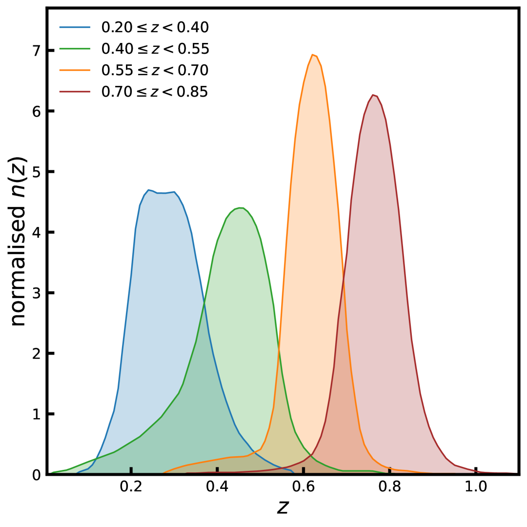
Figure 1: Redshift distribution of four DES tomographic bins computed using DNF algorithm: $0.2\leq 0.4$ (in blue), $0.40\leq 0.55$ (in green), $0.55\leq 0.70$ (in orange) and $0.70\leq 0.85$ (in brown).

The Dark Energy Survey (DES) was a six-year observing programme conducted with the Dark Energy Camera 2015AJ....150..150F mounted on the Blanco $4$-meter telescope at the Cerro Tololo Inter-American Observatory (CTIO) in Chile. The survey covered $5000$ deg² of the southern sky in $grizY$ filters, including the EMU-PS1 footprint. In this study, we utilise the magnitude-limited (MagLim) galaxy sample 2021PhRvD.103d3503P; 2022PhRvD.106j3530P constructed from the first three years of DES observations 2018ApJS..239...18A. The MagLim sample is defined with a cut on the $i-$band magnitude that depends linearly on photometric redshift, $i<4z+18$ 2022PhRvD.105b3520A.

The photometric redshifts for MagLim galaxies were estimated using the Directional Neighbourhood Fitting algorithm (2016MNRAS.459.3078D; 2021ApJS..254...24S, DNF;). The DNF algorithm computes a point estimate $z_{\text{DNF}}$ of each galaxy’s redshift by fitting through the $80$ nearest neighbours in colour-magnitude space constructed from a spectroscopic reference set. This reference set includes objects from $24$ different spectroscopic catalogues, such as the Sloan Digital Sky Survey (SDSS) DR14 2018ApJS..235...42A, the Optical redshifts for the Dark Energy Survey program (2020MNRAS.496...19L, OzDES;), the VIMOS Public Extragalactic Redshift Survey (2014A&A...562A..23G, VIPERS;), and the Physics of the Accelerating Universe photometric catalogue 2019MNRAS.484.4200E. In addition to point estimates, DNF provides individual redshift posterior derived from the fitting residuals 2022PhRvD.106j3530P.

The MagLim sample is divided into six tomographic bins with edges at $z=[0.20,0.40,0.55,0.70,0.85,0.95,1.05]$. However, due to issues identified in the galaxy sample above $z=0.85$ 2022PhRvD.105b3520A, we restrict our analysis to the first four tomographic bins for cross-correlation with EMU-PS1. The number density of galaxies in each of these four bins are provided in Table 1. The corresponding redshift distributions, validated using galaxy clustering cross-correlations 2022MNRAS.513.5517C, are shown in Figure 1. The DES data used in this analysis are publicly available at https://des.ncsa.illinois.edu/.

4 Methodology

Figure 2: Galaxy overdensity maps used in the study. (a) EMU-PS1 raw overdensity map, (b) EMU-PS1 weighted overdensity map following Eq. 9, (c)-(f) DES galaxy overdensity maps in four tomographic bins. The blue contour in DES maps shows the EMU-PS1 footprint. The colorbars indicate the strength of overdensities (in pixels), with masked region shown in grey colour. The grid spacing is $5^{\circ}$ (in both ra and dec) for EMU-PS1, and $30^{\circ}$ for DES.

4.1 Power spectra

The computation of power spectra requires accurately specifying the survey footprint and characterising the fluctuations in observed number of sources due to image noise. The observed galaxy overdensity maps in Eq. 1 is modified to

$$\hat{\delta}_{g}(\hat{\bm{n}})=\frac{\hat{N}_{g}(\hat{\bm{n}})}{\overline{N}_{g}\,w_{g}(\hat{\bm{n}})}-1,$$ (9)

where $w_{g}(\hat{\bm{n}})$ is the weight map which defines the variations in observed number of sources over the survey footprint due to observational noise. $\overline{N}_{g}$ now becomes the weighted mean source density per pixel

$$\overline{N}_{g}=\frac{\langle\hat{N}_{g}(\hat{\bm{n}})\rangle}{\langle w_{g}(\hat{\bm{n}})\rangle},$$ (10)

where $\langle\cdot\rangle$ denotes average over all observed pixels.

The construction of weight maps for EMU-PS1 is described in section 4.1 of T24, while the weights for DES galaxies are available from the public dataset. We build the weighted EMU-PS1 and DES galaxy overdensity maps at HEALPix 2005ApJ...622..759G resolution $N_{\text{side}}=512$ using Eq. 9. To avoid heavily masked pixels, we set both $w_{g}(\hat{\bm{n}})$ and $\delta_{g}(\hat{\bm{n}})$ to zero where $w_{g}(\hat{\bm{n}})<0.5$. The raw and weighted galaxy overdensity maps for EMU-PS1 are shown in Figure 2a and 2b, respectively, while Figures 2c–2f display the DES galaxy overdensity maps for the four tomographic bins.

The computation of angular power spectra via Eq. 3 assumes full sky coverage. However, in practice we only observe a fraction of sky in galaxy surveys, and can only compute the pseudo power spectra. The incomplete sky coverage induces coupling between different harmonic modes. We used a pseudo-$C_{\ell}$ estimator 1973ApJ...185..413P; 2002ApJ...567....2H implemented in NaMaster python code 2019MNRAS.484.4127A to compute the full sky power spectrum from the pseudo power spectrum. The pseudo-$C_{\ell}$ estimator accounts for the harmonic mode coupling by computing the coupling matrix by factoring in the survey area 2002ApJ...567....2H; 2022MNRAS.515.1993S. Using this framework, we compute the EMU-PS1 galaxy auto-power spectrum ($C_{\ell}^{\text{EMU}}$), DES galaxy auto-power spectrum in four tomographic bins ($C_{\ell}^{\text{DES}}$), and the cross-power spectra between EMU-PS1 and DES tomographic bins ($C_{\ell}^{\text{EMU}\times\text{DES}}$).

4.2 EMU source redshift distribution

The theoretical angular power spectra in Eq. 5 requires knowledge of the redshift distribution of EMU-PS1 sources. As described in Section 1, in absence of any direct measurements of redshifts for radio continuum sources, many studies with clustering of radio sources relies heavily on TRECS and SKADS simulations. These simulations include contributions from AGNs and SFGs as the main tracers of radio galaxy populations. Recently, T24 used these simulated redshift distributions to model EMU-PS1 auto-power spectrum and its cross-correlation with CMB lensing convergence.

In this work, we attempt to constrain the redshift distribution of EMU-PS1 sources based on the measured cross-correlation with DES tomographic bins. We examine the efficacy of TRECS and SKADS redshift distributions to model the cross-power spectra. We also consider a parametric model for the EMU-PS1 $n(z)$ to test departures from TRECS and SKADS $n(z)$. The model redshift distribution has three free parameters and is given by

$$n(z)\propto\frac{(z/z_{0})^{2}}{1+(z/z_{0})^{2}}\frac{1}{1+(z/z_{\text{tail}})^{\gamma}}$$ (11)

The parameter $z_{0}$ controls the peak of the redshift distribution, $z_{\text{tail}}$ parametrises the width of the tail and $\gamma$ affects the decay rate of the high redshift tail. The parametric form was used by 2021MNRAS.502..876A to model the distribution of LoTSS DR1 sources. The three parameters model $n(z)$ is motivated by its flexibility to adjust the location of the peak, width of the distribution and properties of the high redshift tail independently. Although the model $n(z)$ given by Eq. 11 may not have the same level of physical motivation as the form used in LoTSS DR2 analysis by 2024A&A...681A.105N, its ability to encompass a wide range of distributions with simple mathematical form makes it a suitable choice for our analysis. It can also reproduce the location of the peaks and long tails for both TRECS and SKADS redshift distributions within its parametrisation.

4.3 Galaxy bias model

The final ingredient required for our analysis is a model of the linear galaxy bias from EMU-PS1 and DES tomographic bins. Following 2022PhRvD.105b3520A and 2022PhRvD.106j3530P, we adopt a linear constant galaxy bias model for DES tomographic bins, $b^{i}(z)=b_{g}^{i}$. For EMU-PS1, different galaxy bias models including constant galaxy bias, constant amplitude galaxy bias, and quadratic galaxy bias were studied in our companion T24 paper. We used here the constant amplitude galaxy bias model parameterised with $b(z)=b_{g}/D(z)$ for the EMU-PS1 galaxy clustering. The constant amplitude model allows for redshift evolution of galaxy bias with only one free parameter, which is an appropriate choice for the small sky coverage of EMU-PS1. With larger sky coverage possible with EMU full survey, we will be able to test galaxy bias models with more than one free parameter.

4.4 Covariance matrix

A robust estimate of covariance matrix for the power spectra is crucial to estimate parameters. We used the measured pseudo-power spectra rescaled with the survey sky fraction ($f_{\mathrm{sky}}^{\mathrm{EMU-PS1}}=0.0065$ and $f_{\mathrm{sky}}^{\mathrm{DES}}=0.1187$) to generate mock EMU-PS1 and DES tomographic fields using GLASS 2023OJAp....6E..11T. We apply the survey selection functions to mock data and bin the simulated power spectra similar to observed data. We create $1000$ mock realisations and compute the sample covariance matrix using the relation

$${\sf K}_{\ell\ell^{\prime}}^{AB,CD}=\frac{1}{{N}_{{s}}-1}\sum_{i=1}^{{N}_{{s}}}\left(\tilde{C}^{AB,i}_{\ell}-\left\langle\tilde{C}_{\ell}^{AB}\right\rangle\right)\left(\tilde{C}^{CD,i}_{\ell}-\left\langle\tilde{C}_{\ell}^{CD}\right\rangle\right),$$ (12)

where $A,B,C,D\in\{g^{\text{DES}},g^{\text{EMU}}\}$, ${N}_{{s}}$ is the total number of simulations, $\tilde{C}^{gg,i}_{\ell}$ is the power spectrum estimated from the $i\text{th}$ simulation and

$$\left\langle\tilde{C}_{\ell}^{gg}\right\rangle=\frac{1}{{N}_{{s}}}\sum_{i=1}^{{N}_{{s}}}\tilde{C}^{gg,i}_{\ell}$$ (13)

The method of computing covariance matrix allows us to include properties of EMU-PS1 field without any assumptions about its source redshift distribution or galaxy bias. We account for the Anderson-Hartlap correction factor when computing the inverse of the sample covariance matrix Anderson2004; 2007A&A...464..399H

$${\sf K}_{\ell\ell^{\prime}}^{-1}\to\frac{{N}_{{s}}-{N}_{{d}}-2}{{N}_{{s}}-2}\,{\sf K}_{\ell\ell^{\prime}}^{-1}$$ (14)

where ${N}_{{d}}$ is the size of the data vector.

4.5 Parameter estimation

As first step, we used maximum likelihood estimation with $C_{\ell}^{\text{DES}}$ to estimate the galaxy bias in independent DES tomographic bins. This enabled us to validate our analysis pipeline by comparing our estimates with previous DES galaxy bias measurements. We, then, used the joint data vector $\bm{d}_{\ell}=\{C_{\ell}^{\text{EMU}\times\text{DES}},C_{\ell}^{\text{EMU}}\}$ to constrain EMU-PS1 $n(z)$ and galaxy bias evolution. The log-likelihood function is given

$$\log\mathcal{L}=-\frac{1}{2}[\bm{d}_{\ell}-\bm{t}_{\ell}(\theta)]^{\top}\,({\sf K}^{-1})_{\ell\ell^{\prime}}\,[\bm{d}_{\ell}-\bm{t}_{\ell}(\theta)],$$ (15)

where $\bm{t}_{\ell}(\theta)$ is the theory vector. $\theta$ represents the set of free parameters; $\theta=\{b_{g}\}$ for analysis TRECS and SKADS $n(z)$, and $\theta=\{b_{g},z_{0},z_{\text{tail}},\gamma\}$ for model $n(z)$ given by Eq. 11. ${\sf K}_{\ell\ell^{\prime}}$ is the joint covariance matrix given by

$${\sf K}_{\ell\ell^{\prime}}=\begin{bmatrix}{\sf K}_{\ell\ell^{\prime}}^{g_{1}g,g_{1}g}&{\sf K}_{\ell\ell^{\prime}}^{g_{1}g,g_{2}g}&{\sf K}_{\ell\ell^{\prime}}^{g_{1}g,g_{3}g}&{\sf K}_{\ell\ell^{\prime}}^{g_{1}g,g_{4}g}&{\sf K}_{\ell\ell^{\prime}}^{g_{1}g,gg}\\ {\sf K}_{\ell\ell^{\prime}}^{g_{2}g,g_{1}g}&{\sf K}_{\ell\ell^{\prime}}^{g_{2}g,g_{2}g}&{\sf K}_{\ell\ell^{\prime}}^{g_{2}g,g_{3}g}&{\sf K}_{\ell\ell^{\prime}}^{g_{2}g,g_{4}g}&{\sf K}_{\ell\ell^{\prime}}^{g_{2}g,gg}\\ {\sf K}_{\ell\ell^{\prime}}^{g_{3}g,g_{1}g}&{\sf K}_{\ell\ell^{\prime}}^{g_{3}g,g_{2}g}&{\sf K}_{\ell\ell^{\prime}}^{g_{3}g,g_{3}g}&{\sf K}_{\ell\ell^{\prime}}^{g_{3}g,g_{4}g}&{\sf K}_{\ell\ell^{\prime}}^{g_{3}g,gg}\\ {\sf K}_{\ell\ell^{\prime}}^{g_{4}g,g_{1}g}&{\sf K}_{\ell\ell^{\prime}}^{g_{4}g,g_{2}g}&{\sf K}_{\ell\ell^{\prime}}^{g_{4}g,g_{3}g}&{\sf K}_{\ell\ell^{\prime}}^{g_{4}g,g_{4}g}&{\sf K}_{\ell\ell^{\prime}}^{g_{4}g,gg}\\ {\sf K}_{\ell\ell^{\prime}}^{gg,g_{1}g}&{\sf K}_{\ell\ell^{\prime}}^{gg,g_{2}g}&{\sf K}_{\ell\ell^{\prime}}^{gg,g_{3}g}&{\sf K}_{\ell\ell^{\prime}}^{gg,g_{4}g}&{\sf K}_{\ell\ell^{\prime}}^{gg,gg}\\ \end{bmatrix}$$ (16)

where we used $g$ to denote EMU-PS1 field and $g_{1}-g_{4}$ denote the four DES tomographic bins. The parameter priors used in our analysis are mentioned in Table 3. We used the EMCEE package 2013PASP..125..306F to effectively sample the parameter space and generate posterior distributions. We put limits on model $n(z)$ such that its tail drops to zero at $z\geq 10$. Additionally, we check the first and second derivatives of our model $n(z)$ to avoid tophat-like distributions of EMU-PS1 sources.

Table 3: The parameters and their priors used in the analysis. Square brackets denote flat priors. $b_{i}^{\text{DES}}$ is the galaxy bias for the $i$th DES tomographic bin and $b_{g}^{\text{EMU}}$ is the galaxy bias for EMU-PS1 radio sources. The parameters $z_{0},z_{\text{tail}},\text{ and }\gamma$ control the EMU-PS1 redshift distribution.

$b_{i}^{\text{DES}}$	$b_{g}^{\text{EMU}}$	$z_{0}$	$z_{\text{tail}}$	$\gamma$
$i\in\{1,4\}$
$[0,5]$	$[0,20]$	$[0,15]$	$[0,15]$	$[0,20]$

5 Pipeline validation

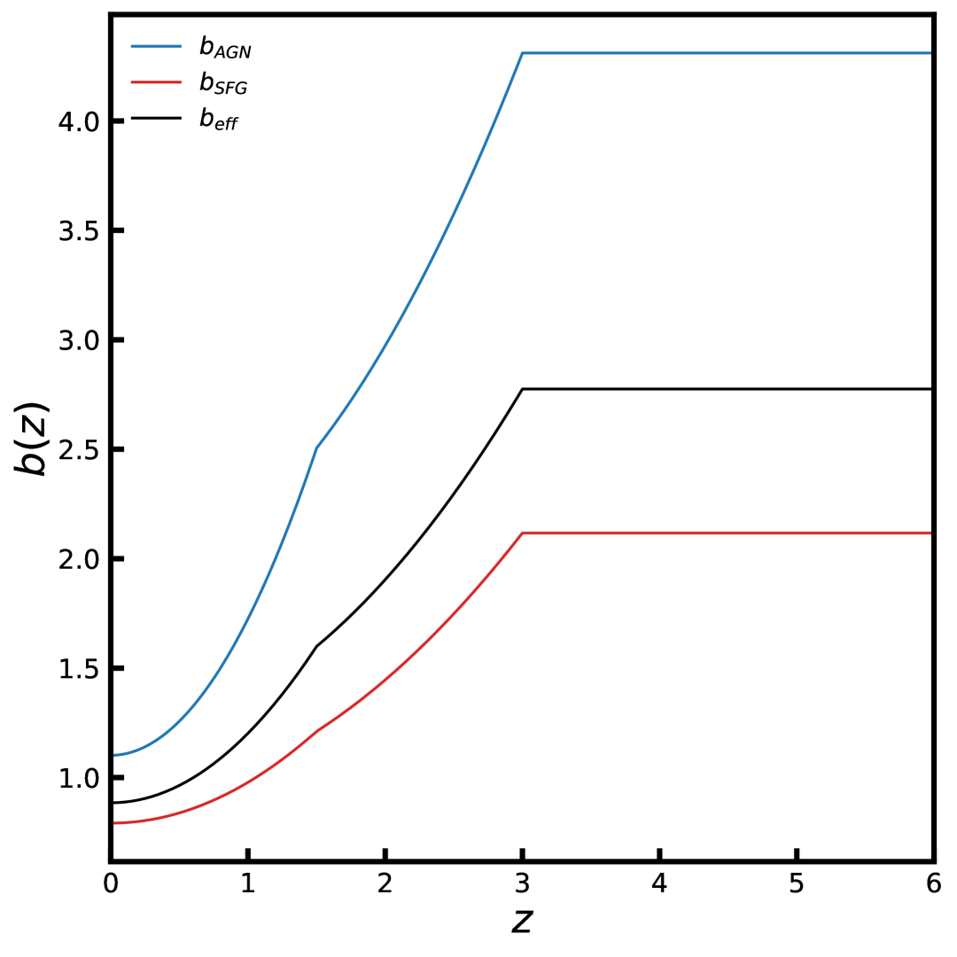
(a)

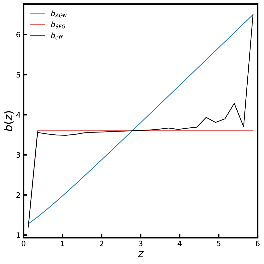
(b)

Figure 3: The two cases of galaxy bias models used for creating mock EMU-PS1 catalogues. The galaxy bias for AGNs is shown in blue, for SFGs in red, and the effective galaxy bias for their joint population is shown in black.

(a)

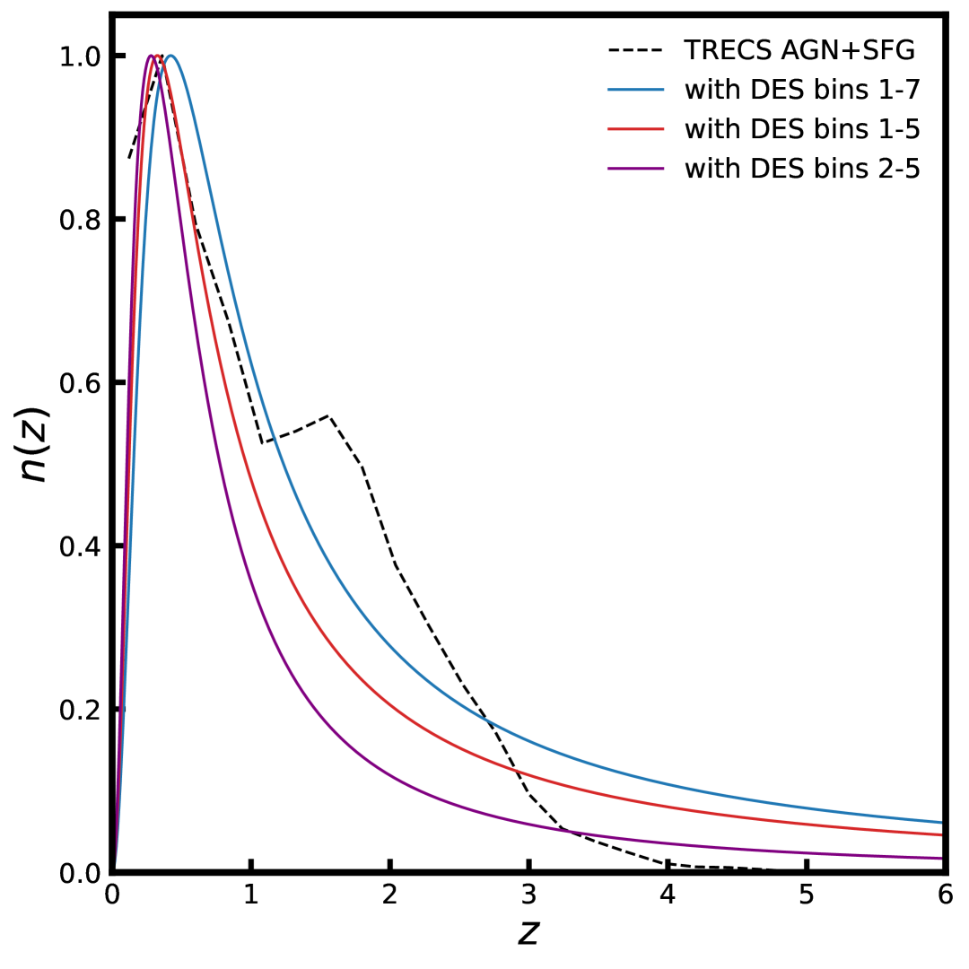
(b)

Figure 4: Best-fit EMU PS1 redshift distributions obtained from simulations considering cross-correlations with different combinations of DES tomographic bins. The black dashed line shows the fiducial redshift distribution of TRECS AGN and SFG joint sample. The redshift distributions are normalised to a unit maximum for illustrative purposes. For description of combinations of DES bins, see Section 5 in the main text.

Before analysing data, it is essential to assess how well our parametric redshift distribution model (Eq. 11) and analysis choices (described in Section 4) can recover the underlying true redshift distribution of EMU-PS1 radio sources. In this section, we test the robustness of our analysis pipeline against internal systematics. To this end, we used GLASS to generate $50$ mock simulations of correlated EMU-PS1 and DES galaxy fields, with seven DES tomographic bins defined over the redshift intervals $z=[0.00,0.20,0.40,0.55,0.70,0.85,0.95,1.05]$. The mocks adopt the same angular coverage as in the data: $\sim 270$ deg² for EMU-PS1 and $\sim 5000$ deg² for DES (as described in Section 3).

For EMU-PS1, we considered AGNs and SFGs as independent populations and used TRECS simulations to obtain their fractional contributions as well as redshift distributions, after applying a flux threshold of $180\,\mu$Jy. However, for analysis we used the joint simulated sample of AGNs and SFGs. We considered two different cases of galaxy bias for AGNs and SFGs for simulations. In the first case we used galaxy bias prescriptions based on different population types (i.e. normal star-forming, starburst, radio-quiet quasar, FRI and FRII radio galaxies) following 2012MNRAS.424..801R. The galaxy bias beyond redshift $z\sim 3$ assumes a constant value to avoid excessive clustering strength at high redshifts. In the second case, we created an ad-hoc model where the SFG galaxy bias rises sharply only up to redshift $z\sim 0.5$, while the AGN bias grows continuously with redshift. We emphasise that the galaxy bias models for AGNs and SFGs in both cases are intended to only probe potential systematic effects in our methodology for estimating the EMU-PS1 redshift distribution. The galaxy biases for AGNs, SFGs and their joint sample for both cases are shown in Figure 3. The $b_{\text{eff}}(z)$ represents the evolution of galaxy bias for the joint sample computed using

$$b_{\text{eff}}(z)=\frac{b_{\text{AGN}}(z)\cdot n_{\text{AGN}}(z)+b_{\text{SFG}}(z)\cdot n_{\text{SFG}}(z)}{n_{\text{AGN}}(z)+n_{\text{SFG}}}$$ (17)

We study three different scenarios in our mock analyses:

1. using all seven DES redshift bins,

2. excluding redshift bins above $z=0.85$

3. using only the four redshift bins between $0.20\leq z<0.85$.

Scenario 1 allows us to test the constraining power of high-redshift ($z>0.85$) data, while scenario 2 helps assess the role of low-redshift bins ($0.0\leq z<0.85$). Scenario 3 replicates the analysis setup used in our main results (see Section 3). In all three cases, we apply the same parametric redshift model (Eq. 11) and galaxy bias (Section 4.3) used for the real data. Figure 4 shows the recovered EMU-PS1 redshift distributions from each of the simulation scenarios in the two cases of galaxy bias models. For galaxy bias model based on different population types (Figure 3(a)), we find a slight preference for a low redshift peak than our fiducial $n(z)$ in scenarios 1 and 2. We recover the peak location of the fiducial $n(z)$ consistently from rest of the mock analyses, despite using incorrect prescriptions for the true EMU-PS1 galaxy bias and redshift distribution. Major differences between the model and input distributions manifest primarily in the high-redshift tail, including features such as the bump around $z\sim 1.7$. These results from simulations provide a strong validation for our methodology and motivates recovering at least the peak of the true EMU-PS1 redshift distribution from real data.

6 Results

6.1 Power spectra and detection significance

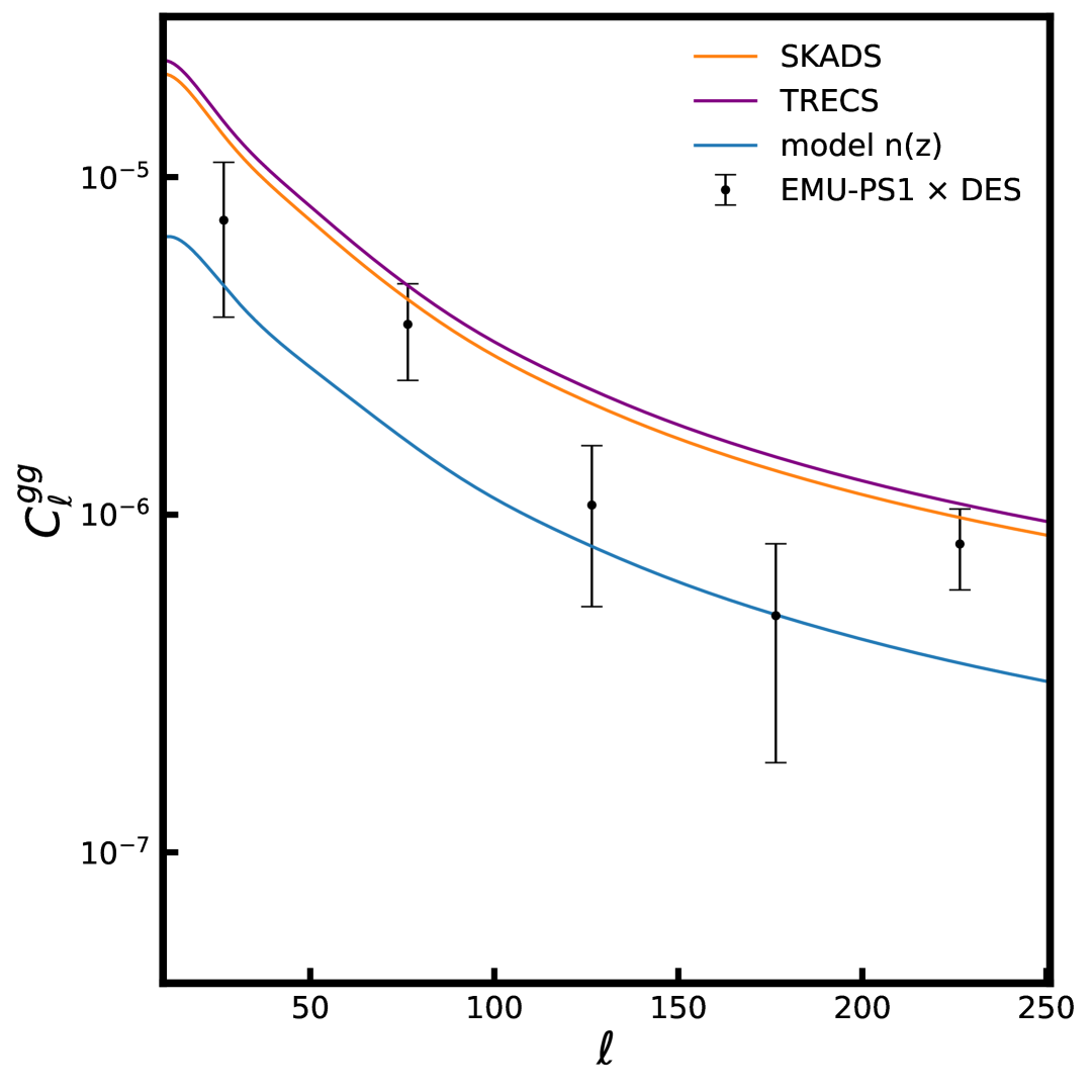
(a) EMU-PS1 $\times$ DES Bin 1

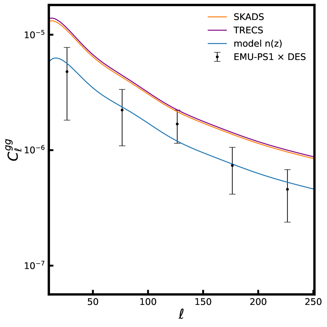
(b) EMU-PS1 $\times$ DES Bin 2

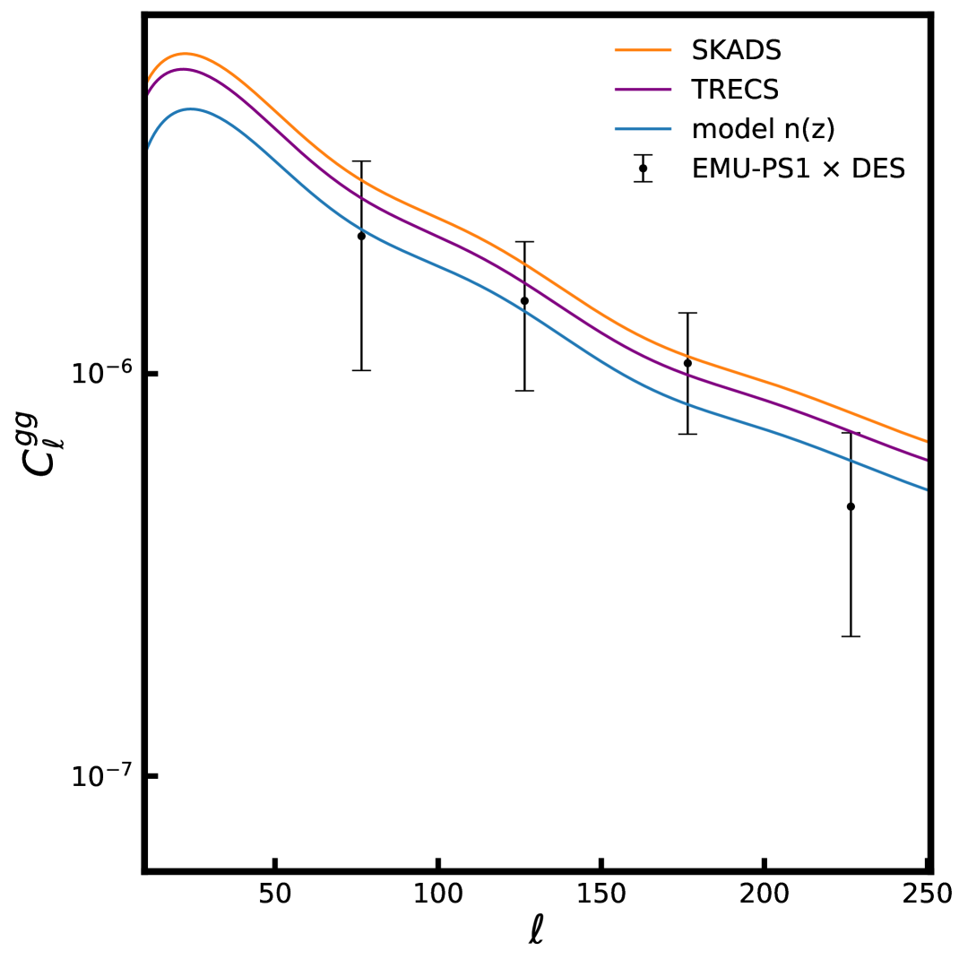
(c) EMU-PS1 $\times$ DES Bin 3

(d) EMU-PS1 $\times$ DES Bin 4

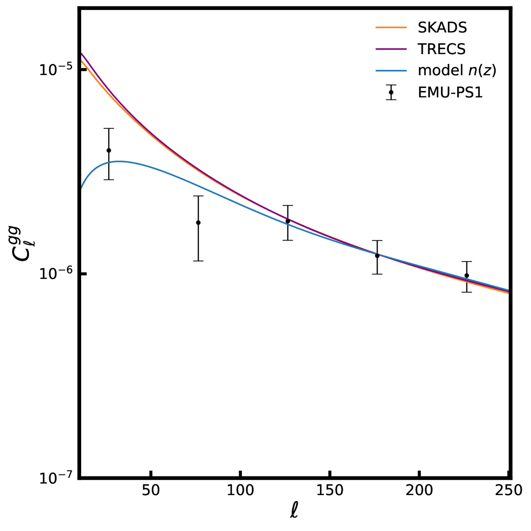
(e) EMU-PS1 $\times$ EMU-PS1

Figure 5: The angular power spectra measured from cross-correlation between EMU-PS1 and DES tomographic bins (a-d) and EMU-PS1 auto-power spectrum (e). The best-fit power spectra obtained using SKADS and TRECS $n(z)$ are shown in orange and purple, respectively. The best-fits from our model $n(z)$ are shown with the blue curve. The $1\sigma$ errors on data points are computed from the diagonal of the sample covariance matrix (Eq. 12).

The EMU-PS1 auto-power spectrum ($C_{\ell}^{\text{EMU}}$) and the cross-power spectra with DES tomographic bins ($C_{\ell}^{\text{EMU}\times\text{DES}}$), measured over the multipole range $2\leq\ell\leq 250$, are shown in Figure 5 as black data points. The power spectra are binned into five linear multipole intervals with bin width $\delta\ell=50$. We apply a conservative upper multipole cut at $\ell=250$ to restrict our analysis to linear scales. Beyond this range, the contribution from multi-component radio sources also begins to dominate the EMU-PS1 power spectrum (see T24), and a detailed treatment to mitigate these effects is beyond the scope of this work.

The standard $1\sigma$ uncertainties on the power spectra measurements are computed from the diagonal of the sample covariance matrix defined in Eq. 12. We note that the data point at $\ell=26$ in EMU-PS1 $\times$ DES Bin 3 power spectrum (Figure 5c) is found to be negative, and hence is absent from the Figure. Assuming the null hypothesis of zero correlation, the significance of detecting the $C_{\ell}^{\text{EMU}\times\text{DES}}$ power spectra was computed using $\smash{\sqrt{\chi^{2}_{\text{null}}-\chi^{2}_{\text{best-fit}}}}$. The resulting detection significances for the four DES tomographic bins are $5.5\sigma,\,5.4\sigma,\,4.5\sigma$ and $4.6\sigma$, respectively for Bins 1 through 4.

6.2 DES galaxy bias

Before estimating EMU-PS1 galaxy bias and redshift distribution, we need precise constraints on the DES galaxy bias. We start by binning the measured tomographic $C_{\ell}^{\text{DES}}$ power-spectra in eight linear multipole bins between $2\leq\ell\leq 250$. We then use maximum likelihood estimation framework (see section 4.5) to determine linear galaxy bias in each DES tomographic bin. As shown in Figure 6, our estimates of DES linear galaxy bias are consistent with previous measurements from 2022PhRvD.105b3520A within $1\sigma$ uncertainties. We note that while 2022PhRvD.105b3520A employed a full $3\times 2$-point analysis to estimate galaxy bias, our results are based solely on galaxy clustering measurements. This can yield tighter constraints on the galaxy bias due to the reduced number of nuisance parameters that need to be marginalized over, compared to a full $3\times 2$-pt analysis. Table 4 lists the best-fit total chi-square value for each of the four DES tomographic bins as a measure of their goodness of fit.

For the purposes of this study, a linear galaxy bias model for the DES tomographic bins is adequate. However, future analyses using the EMU main survey will benefit from a larger sky area. To optimally utilize the cross-correlation measurements, a non-linear prescription for DES galaxy bias (as used in 2022PhRvD.106j3530P) will be necessary to improve constraints on the redshift distribution of radio sources.

Figure 6: Galaxy bias estimated for the four DES tomographic bins. The effective redshift is shifted for illustrative purposes only.

6.3 EMU-PS1 redshift distribution and galaxy bias

6.3.1 With SKADS and TRECS

The SKADS and TRECS simulations do not provide fluxes directly at the EMU observation frequency of $944$ MHz. To address this, we interpolate the available fluxes between the provided frequency bands in both simulations to estimate the flux at 944 MHz. We, then, apply a flux cut at $180\,\mu$Jy to construct the appropriate redshift distributions and estimate the amplitude of galaxy bias $b_{g}$ through a joint analysis of $C_{\ell}^{\text{EMU}\times\text{DES}}$ and $C_{\ell}^{\text{EMU}}$ power spectra. In Figure 7, we show the posterior distributions of $b_{g}$ along-with their best-fit values. We note that the SKADS $n(z)$ model has a prominent, slowly decaying tail compared to that from TRECS (see Figure 9). As a result, to achieve a comparable fit to the observed power spectra, the SKADS model requires a higher value of $b_{g}$, which is indeed what we find. Our estimates of EMU-PS1 galaxy bias are consistent with previous measurements from T24, albeit with uncertainties that are approximately three times smaller. This improvement is expected given our use of a larger dataset cross-correlating the EMU-PS1 map with four tomographic DES maps instead of just using the EMU-PS1 auto-power spectrum.

The best-fit theoretical power spectra are shown in Figure 5. We find that the cross-power spectra $C_{\ell}^{\text{EMU}\times\text{DES}}$ in the the higher redshift bins (bins 3 and 4) are well fit by both SKADS and TRECS $n(z)$ models. However, both models fail to provide good fits in the lower redshift bins (bins 1 and 2). We obtained a total $\chi^{2}$ value of $86.30$ for TRECS and $78.03$ for SKADS, with $\nu=24$ degrees of freedom. This discrepancy indicates that the data favour a different redshift evolution at low $z$ than is represented by either SKADS or TRECS.

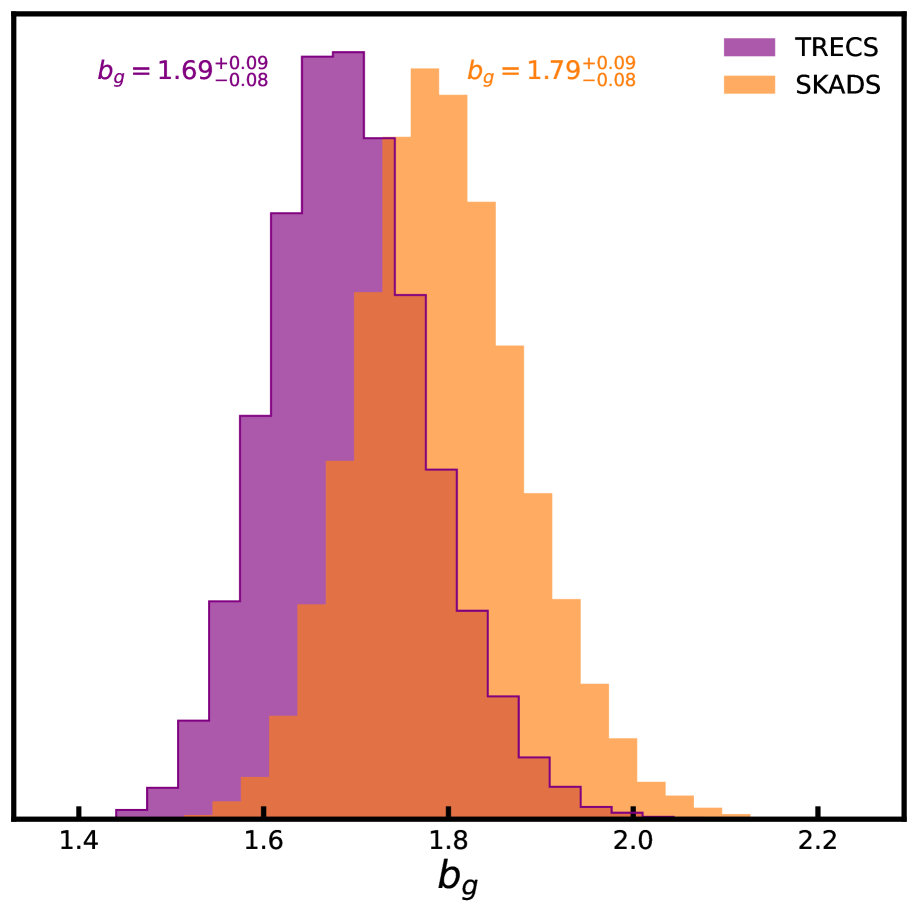
Figure 7: Posteriors for EMU-PS1 galaxy bias assuming TRECS (in purple) and SKADS (in orange) redshift distributions. The quoted values are median of the posteriors with $\pm 1\sigma$ errors.

6.3.2 With model $n(z)$

We adopted the model redshift distribution from LoTSS DR1 analysis 2021MNRAS.502..876A with parametric form given in Eq. 11, to infer the distribution of EMU-PS1 radio sources. The parameter posteriors with best-fit values and $16^{\text{th}}$ and $84^{\text{th}}$ percentiles are shown in Figure 8. In Figure 9, we compare our resulting best-fit redshift distribution (in blue) with other radio continuum surveys after applying appropriate flux thresholds (assuming a spectral index of 0.75). The shaded region shows the $1\sigma$ uncertainty in our best-fit EMU-PS1 $n(z)$. Notably, most of the variation lies in the amplitude rather than the shape of the distribution. Since clustering measurements are primarily sensitive to the shape of $n(z)$, the deviation of our best-fit distribution from the TRECS and SKADS models at low redshift is particularly significant. However, due to the lack of cross-correlation data at $z>0.85$, the high-redshift tail remains weakly constrained. Despite this, the effective redshift of the inferred distribution (computed using Eq. 18) is well constrained, as shown by its posterior distribution in Figure 10.

$$z_{\text{eff}}=\frac{\int\mathrm{d}z\,z\,n^{2}(z)\,\chi^{2}(z)/H(z)}{\int\mathrm{d}z\,n^{2}(z)\,\chi^{2}(z)/H(z)}\;.$$ (18)

Our best-fit EMU-PS1 $n(z)$ presents a contradictory picture of the redshift distribution of radio sources with peak at a higher redshift of $z_{\text{peak}}\sim 1.5$. The redshift distributions from simulated catalogues of SKADS (shown in orange dashed line) and TRECS (shown in purple dashed line) peak at a significantly lower redshift ($z\lesssim 0.6$). The redshift distribution from LOFAR deep fields 2021A&A...648A...4D; 2024A&A...692A...2B also prefers a low-redshift peak at $z\lesssim 0.6$. However, our findings are in better agreement with the redshift distributions from COSMOS 3GHz survey 2017A&A...602A...5N; 2017A&A...602A...6S and the MeerKAT International GHz Tiered Extragalactic Exploration (MIGHTEE) Survey 2024MNRAS.527.3231W peak at redshift $z\sim 1$. The redshifts of MIGHTEE sources are based on visual cross-match and a likelihood ratio analysis applied to the UltraVISTA $K_{s}$ band selected catalogue 2012A&A...544A.156M. Their analysis reveals a significantly larger number of AGNs at $z\sim 1$ than predicted by simulations, shifting the distribution’s peak to $z\sim 0.94$.

The fits to the angular power spectra $C_{\ell}^{\text{EMU}\times\text{DES}}$ and $C_{\ell}^{\text{EMU}}$ from our best-fit model $n(z)$ are shown with blue curves in Figure 5. We can immediately notice the improvements in power spectra fits compared to TRECS and SKADS. We obtained a total $\chi^{2}=27.65$ for the joint-data vector with our model $n(z)$ having $\nu=21$ degrees of freedom. For reference, the best-fit $\chi^{2}$ values from individual fits are listed in Table 4.

In Section 5, we demonstrated that our methodology reliably recovers the true location of the peak of the EMU-PS1 $n(z)$ and that this result is robust against the specific combination of DES redshift bins used in the cross-correlation analysis. This strengthens the credibility of our finding and reduces the likelihood of misidentification of the peak. We list below several plausible explanations for the high-redshift peak of the EMU-PS1 radio sources:

• A greater population of radio-quiet AGNs at intermediate redshifts ($z\sim 1$–$2$): As suggested by MIGHTEE survey, the abundance of such AGNs at $z\sim 1-2$ may be underestimated in current simulations or overlooked in other radio continuum surveys. Because our method relies solely on measured cross-correlations between EMU-PS1 and DES galaxies, it is potentially more sensitive to the true redshift distribution of AGNs than those recovered from traditional cross-matching techniques.

• Residual systematics in DES redshift distributions or galaxy bias evolution: Although we use the official DES $n(z)$ distributions, known systematics at $z>0.85$ have been reported in the DES tomographic bins 2022PhRvD.105b3520A. Furthermore, uncertainties in photometric redshifts can bias the inferred mean and width of the distributions, leaving room for unidentified systematic errors that could affect our analysis.

• Redshift bin misclassification in DES due to photometric uncertainties: Errors in assigning galaxies to tomographic bins due to photometric redshift uncertainties can bias the inferred clustering signals and distort conclusions drawn from angular power spectra 2024A&A...687A.150S; 2024A&A...690A.338S.

• Survey area limitations and selection effects: Although less likely, it is possible that our unconventional $n(z)$ peak is a result of selection effects or sample variance due to the relatively small area covered by EMU-PS1.

A detailed investigation of these possibilities is beyond the scope of the present work. However, future analyses using the main EMU survey—with its significantly larger sky coverage—will be instrumental in testing these hypotheses and further constraining the redshift distribution of radio sources.

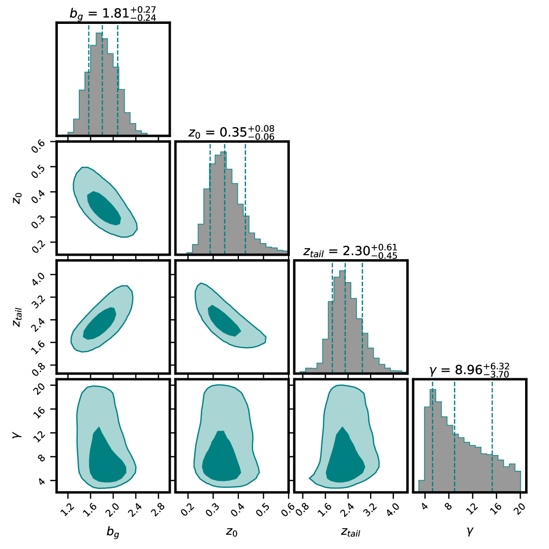
Figure 8: Parameter posteriors obtained from joint analysis of $C_{\ell}^{\text{EMU}\times\text{DES}}$ and $C_{\ell}^{\text{EMU}}$ assuming model $n(z)$ given by Eq. 11. The vertical lines mark the median of the posteriors with $16^{\text{th}}$ and $84^{\text{th}}$ percentiles as errors.

Figure 9: Best-fit redshift distribution (Eq. 11) obtained from cross-correlating EMU-PS1 sources with DES MagLim galaxy sample (shown with solid blue curve). The TRECS and SKADS $n(z)$ are shown in purple and orange, respectively. The redshift distributions from LOFAR deep fields (in green), COSMOS 3GHz (in yellow) and MIGHTEE survey (in red) are shown for comparison.

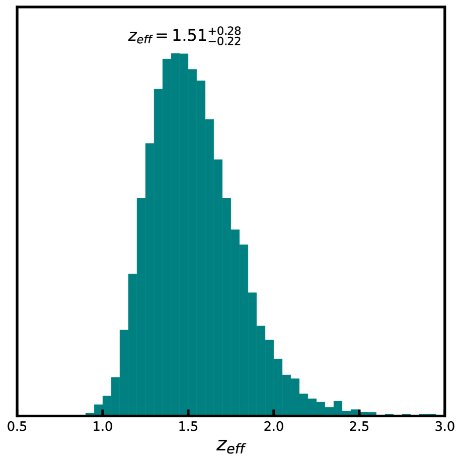
Figure 10: The posterior of the effective redshift of the model redshift distribution computed using Eq. 18.

Table 4: Total chi-square values from the best-fits obtained for DES galaxy-auto power spectra in four redshift bins, EMU-PS1 auto-power spectra and their cross-correlation. $b_{g}$ is the best-fit galaxy bias for DES tomographic bins and EMU-PS1 radio sources with model $n(z)$. The $\chi^{2}_{\text{bf}}$ values correspond to our baseline analysis with best-fit model $n(z)$, whereas $\chi^{2}_{\text{TRECS}}$ and $\chi^{2}_{\text{SKADS}}$ are for TRECS and SKADS $n(z)$, respectively. The number of degrees of freedom for $C_{\ell}^{\text{DES}}$ is $\nu=7$ in every redshift bin. For the joint analysis of $C_{\ell}^{\text{EMU}\times\text{DES}}$ and $C_{\ell}^{\text{EMU}}$, $\nu=24$ with TRECS or SKADS, and $\nu=21$ for model $n(z)$.

		$b_{g}$	$\chi^{2}_{\text{bf}}$	$\chi^{2}_{\text{TRECS}}$	$\chi^{2}_{\text{SKADS}}$
	Bin 1	$1.37^{+0.04}_{-0.04}$	$9.17$	-	-
$C_{\ell}^{\text{DES}}$	Bin 2	$1.73^{+0.05}_{-0.05}$	$10.82$	-	-
	Bin 3	$1.74^{+0.05}_{-0.05}$	$8.08$	-	-
	Bin 4	$1.67^{+0.05}_{-0.05}$	$8.86$	-	-
$C_{\ell}^{\text{EMU}}$	-	$1.81^{+0.27}_{-0.24}$	$2.98$	$20.99$	$18.11$
	Bin 1	-	$5.98$	$23.93$	$16.06$
$C_{\ell}^{\text{EMU}\times\text{DES}}$	Bin 2	-	$3.95$	$22.41$	$19.03$
	Bin 3	-	$7.36$	$10.66$	$13.64$
	Bin 4	-	$7.38$	$8.31$	$11.20$

7 Conclusion

In this work, we measured the angular power spectra from the cross-correlations between EMU-PS1 radio sources and DES photometric galaxies. By combining these cross-power spectra with the EMU-PS1 auto-power spectrum, we inferred the redshift distribution of EMU-PS1 radio sources.

We applied a flux cut of $180\mu$Jy to the EMU-PS1 source catalogue, which was generated using the PyBDSF source detection algorithm. We then constructed weights for EMU-PS1 to account for the variations in source counts due to observational noise. Subsequently, we cross-correlated the weighted radio catalogue with the DES MagLim galaxy sample, which was divided into four tomographic bins in the redshift range $0.2\leq z<0.85$. The angular power spectra were measured using the NaMaster pseudo-$C_{\ell}$ estimator.

We estimated the galaxy bias in the DES tomographic bins from their auto-power spectrum. For EMU-PS1, we adopted a constant-amplitude galaxy bias model along with a parametric form for its redshift distribution, following 2021MNRAS.502..876A. We also compared the performance of our baseline model $n(z)$ with the widely used simulated redshift distributions from SKADS and TRECS. The free parameters in our models were constrained using MCMC analysis with EMCEE. We prepared mock catalogues of correlated EMU-PS1 and DES surveys to validate our analysis pipeline, as described in Section 5. Our validation confirmed that our methodology is robust in identifying the peak location of the EMU-PS1 redshift distribution. The key findings of our study are summarized below:

• The cross-power spectra between EMU-PS1 and DES bins were detected with $11\sigma,\,8\sigma,\,7\sigma$ and $7.5\sigma$ significance, respectively, for $\ell<250$.

• Our estimates of DES galaxy bias, based solely on galaxy clustering measurements, are consistent with previous studies using the $3\times 2$-pt analysis 2022PhRvD.105b3520A.

• We found that TRECS and SKADS $n(z)$ do not adequately reproduce the cross-power spectra in the first two DES redshift bins. We obtained a total $\chi^{2}$ value of $86.30$ for TRECS and $78.03$ for SKADS, with $\nu=24$ degrees of freedom.

• The EMU-PS1 redshift distribution obtained from our baseline model $n(z)$ (Eq. 11) fits the data significantly better than either TRECS or SKADS. Our best-fit model $n(z)$ shows a peak at $z\sim 1.5$, which is notably higher than the peaks of TRECS and SKADS simulations. The difference in the recovered distribution at low redshifts explains the poor fits from simulated $n(z)$ models.

• The tail of our best-fit $n(z)$ distribution agrees very well with TRECS, although there is larger uncertainty in the high-redshift tail due to the lack of cross-correlation data for $z>0.85$.

• With our model $n(z)$, we found a galaxy bias value of $b_{g}=1.81^{+0.27}_{-0.24}$, which is consistent with previous findings from T24. The total chi-square value for the joint data vector was $27.65$, with $\nu=21$ degrees of freedom.

The limitations of radio continuum surveys in directly measuring the redshift distribution of sources can be partially mitigated through cross-correlation measurements. This paper highlights the potential for directly inferring the radio sources’ $n(z)$ through cross-correlation with optical surveys. With additional high-redshift data from optical/near-infrared surveys such as Euclid, the Vera C. Rubin Observatory LSST 2009arXiv0912.0201L; 2019ApJ...873..111I, and 4MOST 2019Msngr.175....3D, tighter constraints on the radio source $n(z)$ can be achieved. This, in turn, will enhance the prospects for cosmological studies using the ongoing EMU main survey and the SKA in the future.

Acknowledgments

The Australian SKA Pathfinder is part of the Australia Telescope National Facility which is managed by CSIRO. Operation of ASKAP is funded by the Australian Government with support from the National Collaborative Research Infrastructure Strategy. ASKAP uses the resources of the Pawsey Supercomputing Centre. Establishment of ASKAP, the Murchison Radio-astronomy Observatory and the Pawsey Supercomputing Centre are initiatives of the Australian Government, with support from the Government of Western Australia and the Science and Industry Endowment Fund. We acknowledge the Wajarri Yamatji people as the traditional owners of the Observatory site.

Funding Statement

BB-K acknowledges support from INAF for the project ‘Paving the way to radio cosmology in the SKA Observatory era: synergies between SKA pathfinders/precursors and the new generation of optical/near-infrared cosmological surveys’ (CUP C54I19001050001). CLH acknowledges support from the Hintze Family Charitable Foundation through the Oxford Hintze Centre for Astrophysical Surveys. KT is supported by the STFC grant ST/W000903/1 and by the European Structural and Investment Fund. SC acknowledges support from the Italian Ministry of University and Research (mur), PRIN 2022 ‘EXSKALIBUR – Euclid-Cross-SKA: Likelihood Inference Building for Universe’s Research’, Grant No. 20222BBYB9, CUP C53D2300131 0006, from the Italian Ministry of Foreign Affairs and International Cooperation (maeci), Grant No. ZA23GR03, and from the European Union – Next Generation EU. JA is supported by MICINN (Spain) grant PID2022-138263NB-I00 (AEI/FEDER, UE) and the Diputación General de Aragón-Fondo Social Europeo (DGA-FSE) Grant No. 2020-E21-17R of the Aragon Government.

Data Availability Statement

The DES MagLim data used in this paper is publicly available at https://des.ncsa.illinois.edu/. The EMU Pilot Survey 1 images and source catalogues can be downloaded from the CSIRO ASKAP Science Data Archive (https://research.csiro.au/casda/).