Image Segmentation via Variational Model Based Tailored UNet: A Deep Variational Framework
Abstract
Traditional image segmentation methods, such as variational models based on partial differential equations (PDEs), offer strong mathematical interpretability and precise boundary modeling, but often suffer from sensitivity to parameter settings and high computational costs. In contrast, deep learning models such as UNet, which are relatively lightweight in parameters, excel in automatic feature extraction but lack theoretical interpretability and require extensive labeled data. To harness the complementary strengths of both paradigms, we propose Variational Model Based Tailored UNet (VM_TUNet), a novel hybrid framework that integrates the fourth-order modified Cahn–Hilliard equation with the deep learning backbone of UNet, which combines the interpretability and edge-preserving properties of variational methods with the adaptive feature learning of neural networks. Specifically, a data-driven operator is introduced to replace manual parameter tuning, and we incorporate the tailored finite point method (TFPM) to enforce high-precision boundary preservation. Experimental results on benchmark datasets demonstrate that VM_TUNet achieves superior segmentation performance compared to existing approaches, especially for fine boundary delineation.
Keywords Image segmentation deep learning variational model UNet
1 Introduction
Image segmentation is dividing an image into distinct regions or segments to simplify its representation, making it easier to analyze or interpret. This technique is crucial in various fields, such as medical imaging for detecting tumors, autonomous driving for recognizing roads and obstacles, and video surveillance or scene analysis in computer vision. Traditional methods of image segmentation encompass approaches like thresholding, histogram-based bundling, region growing, k-means clustering, watersheds, active contours, graph cuts, conditional and Markov random fields, and sparsity-based methods minaee2021image . Despite their widespread use, traditional models face challenges when dealing with noise, complex backgrounds, and irregular object shapes. They rely on manually engineered features and mathematical models, such as variational techniques which utilize PDEs.
Using variational energy minimization and PDE-based frameworks has a long history of addressing image segmentation problems and has achieved mickle admirable results chan2001active ; liu2022two ; yang2019image ; zhu2013image . Translate segmentation challenges into energy minimization problems, where the goal is to find an optimal segmentation function that minimizes a designed energy functional as
| (1) |
where represent the segmentation result, which can take one of several forms: a level set function, a region indicator function or a boundary curve, and denotes the input image. The first term of Eq. (1) measures how well the segmentation matches the observed image characteristics and the second enforces smoothness constraints to prevent fragmented or irregular segmentation results. By solving this optimization problem, we can obtain a segmentation result that balances the internal similarity and edge smoothness of the image. Variational PDE-based models excel in image segmentation through their data efficiency, inherent noise robustness, computational lightness, interpretable energy minimization framework, topological adaptability, seamless physical prior integration, and unsupervised operation capability which have been proved in many aspects.
Despite their strong mathematical and physical foundations, PDE-based approaches can be challenging to apply effectively due to their sensitivity to initial setups and the requirement for manual parameter calibration. Manual parameter tuning is labor-intensive, and inappropriate settings, especially on noisy or textured images, can easily lead to under-segmentation or over-segmentation mumford1989optimal . Like Chan-Vese model and other variants based on it, average intensities need manually set update format chan2001active ; vese2002multiphase ; zhang2010active . With the surge of deep learning, its application in image segmentation has revolutionized the field, enabling unprecedented accuracy and efficiency in tasks such as medical imaging, autonomous driving, and remote sensing. Deep learning models, particularly parameter-efficient convolutional neural networks (CNNs) and architectures like FCN long2015fully , UNet ronneberger2015u , and so on, excel at automatically extracting hierarchical features from images, which eliminate the need for handcrafted features. This adaptability allows them to handle complex and diverse datasets with ease. Additionally, deep learning methods support end-to-end learning, reducing the reliance on manual parameter tuning and enabling scalable solutions. Their ability to generalize across various domains and achieve state-of-the-art performance makes them a powerful tool for image segmentation, despite challenges such as the need for large labeled datasets and computational resources.
In this study, we present VM_TUNet, a novel approach that integrates deep learning with variational models for more effective image segmentation. By combining the Cahn-Hilliard equation with the UNet architecture, we create a hybrid model that overcomes the challenges of conventional methods, such as manual parameter tuning and sensitivity to initial conditions. Our approach benefits from the interpretability of variational models and the flexibility and scalability of deep learning, which provides a robust solution to complex image segmentation tasks. This work aims to provide a more adaptable and efficient model for diverse applications, particularly in fields like medical imaging and autonomous driving. Our contributions are threefold:
-
•
Integration of deep learning with traditional variational models: VM_TUNet model proposed in this paper integrates traditional variational models with deep learning methods based on the UNet architecture, which combines the advantages of these two directions.
-
•
Cahn-Hilliard equation to ensure boundary preservation: VM_TUNet employs the fourth-order modified Cahn-Hilliard equation to ensure accurate boundary preservation and allow the model to be more adaptable to different types of data in complex scenarios.
-
•
Tailored finite point method to compute accurately and effectively: VM_TUNet utilizes TFPM to compute the laplacian operator during the segmentation process, which reduces parameter sensitivity and improves computational accuracy and efficiency.
2 Related work
2.1 Variational models
Variational models play a crucial role in image segmentation by leveraging energy minimization and mathematical optimization techniques. Variational approaches to image segmentation commonly involve evolving active contours to precisely delineate the boundaries of objects caselles1997geodesic ; chan2001active ; kass1988snakes . In addition to curve evolution techniques, numerous region-based image segmentation models exist, with the Mumford-Shah variational model being one of the most renowned which has many variants such as Chan-Vese model. Moreover, the use of Euler’s elastica is prevalent in the development of variational methods for mathematical imaging bae2017augmented ; shen2003euler ; tai2011fast ; zhu2013image . Variational approaches offer transparency and interpretability, which make them suitable for medical image analysis. However, their performance can be highly dependent on initialization and often requires manual parameter tuning, which limits the generalization of these methods and they typically processes only one image at a time, which makes them inefficient for relatively large-scale tasks.
2.2 Deep learning models
The development of deep learning has revolutionized image segmentation, which enables outstanding performance in areas such as medical imaging, autonomous driving, and remote sensing. FCN long2015fully and similar models have significantly advanced the use of deep learning architectures in the field of image semantic segmentation. Leading models including UNet ronneberger2015u , SegNet badrinarayanan2017segnet , UNet++ Zhou2018UNetAN , DeepLabV3+ Chen_2018_ECCV and Segment Anything model kirillov2023segment ; zhang2024segment that excel in tasks requiring high accuracy and scalability, which leverage large datasets and powerful computational resources. In contrast to traditional variational models, deep learning provides greater flexibility in handling complex data, automates feature extraction, and supports end-to-end learning, which eliminates the need for manual parameter adjustment. Deep learning methods, however, often necessitate large-scale labeled datasets and significant computational resources, and their complex, non-intuitive nature can reduce interpretability. Overall, while deep learning dominates modern image segmentation due to its performance and flexibility, variational models remain valuable for specific applications where interpretability and theoretical rigor are prioritized.
2.3 Deep learning-enhanced variational models
Inspired by the advantages of both traditional mathematical models and data-driven methods, there is potential to incorporate robust mathematical principles and tools into neural networks for image segmentation tasks celledoni2021structure ; lu2018beyond ; ruthotto2020deep ; weinan2017proposal . A direct approach to achieving this integration involves incorporating functions derived from various PDE models into the loss function chen2019learning ; kim2019cnn ; le2018reformulating . These techniques, called loss-inserting methods, tackle the challenge of numerous PDEs lacking defined energy properties and not being representable as gradient flows of explicit energy. Researchers have also explored modifying neural network architectures to improve their interpretability chen2015learning ; cheng2019darnet ; lunz2018adversarial ; marcos2018learning ; ruthotto2020deep . For example, Liu et al. introduce Inverse Evolution Layers, a novel physics-informed regularization approach that integrates PDEs into deep learning frameworks to enhance image segmentation by embedding physical priors and improving model interpretability liu2025inverse . Nevertheless, introducing physics-informed loss and regularization would greatly increase the difficulty of model training.
Recently, in AAM-39-4 ; tai2024pottsmgnet , theoretical and practical connections between operator-splitting methods and deep neural networks demonstrate their synergistic application in improving image segmentation tasks through efficient optimization and enhanced model interpretability. Based on the split Bregman algorithm for the Potts model, PottsNN integrates a total variation regularization term from Fields of Experts and parameterizes the penalty parameters and thresholding function of the model making manual settings trainable cui2024trainable ; wang2024pottsnn . After PottsMGNet, Double-well Nets bridge the extension of the Allen-Cahn type Merriman-Bence-Osher scheme and neural networks to solve the Potts model which is widely approximated using a double-well potential liu2024double . The above models are all low-order while the higher-order Cahn-Hilliard equation can better maintain the boundary.
3 Problem settings and preliminaries
Cahn-Hilliard equation is important in science and industry, whose fourth-order term ensures smooth boundaries and noise robustness, especially in image segmentation tasks. The corresponding modified Cahn-Hilliard model has been proposed in the study of the diffusion of droplets on solid surfaces and the repulsion and competition between biological populations. Scholars systematically studied the Cahn-Hilliard equation and have established mathematical theories about it; see in Appendix C.2).
Here, we consider the modified Cahn-Hilliard model. Given image and the corresponding segmented image , we consider the following Cahn-Hilliard type equation for binary image segmentation
| (2) |
which can be simplified to the following minimization problem as
where , satisfies on , , and , are two constants that can be assigned using some strategy. These parameters depend on manual experience and affect the results strongly. For example, when the value range of image is , we can initially set , , then solve the steady-state solution of Eq. (2) and update , according to the following formula yang2019image
where the aforementioned model can also be extended for color image segmentation, as demonstrated in yang2019image .
However, the above strategy suffers from parameter sensitivity, lack of adaptability, and heavy reliance on prior knowledge, leading to inconsistent results and high computational costs in complex scenarios. Furthemore, the implementation of modified complex Cahn-Hilliard equations facilitates multi-phase segmentation in wang2022multi .
Define
| (3) |
where inspired by the approximation theory of deep neural network, we will use UNet class architecture to represent as a subnetwork to avoid manual setting and adjustment of parameters like Double-well Net Bao2023ApproximationAO ; liu2024double . Then we have to solve the following equation
| (4) |
4 Method
4.1 Adaption to deep learning framework
For convenience, we convert Eq. (4) into two coupled second-order parabolic equations
| (5) | ||||
where and satisfy . For spatial discretization, we use spatial steps for some and simultaneously, let be the time step, for , then we have the outcome and at every substep. Set where is the sigmoid function and , are the convolution kernel and bias. We propose using a convolutional layer followed by a sigmoid function to generate an initial condition and then solve Eq. (5) until a finite time and use as the final segmentation result.
Thus, we can obtain
| (6) |
and
| (7) |
For at every substep, we directly compute it as the following scheme from Eq. (6)
| (8) |
and for at every substep, we use a one-step forward Euler scheme to time discretize Eq. (7)
| (9) |
Suppose now that we are given a training set of images with their foreground-background segmentation masks and we will learn a data-driven operator so that for any given image with similar properties as the training set, the steady state of Eq. (4) is close to its segmentation . Denote as the collection of all parameters to be determined from the data, i.e., the parameters in and then from Eq. (9) only depends on and . Furthermore, we will determine by solving
where is a loss function which could be the loss functional including hinge loss, logistic loss, and norm, measuring the differences between its arguments rosasco2004loss .
4.2 Variational Model Based Tailored UNet
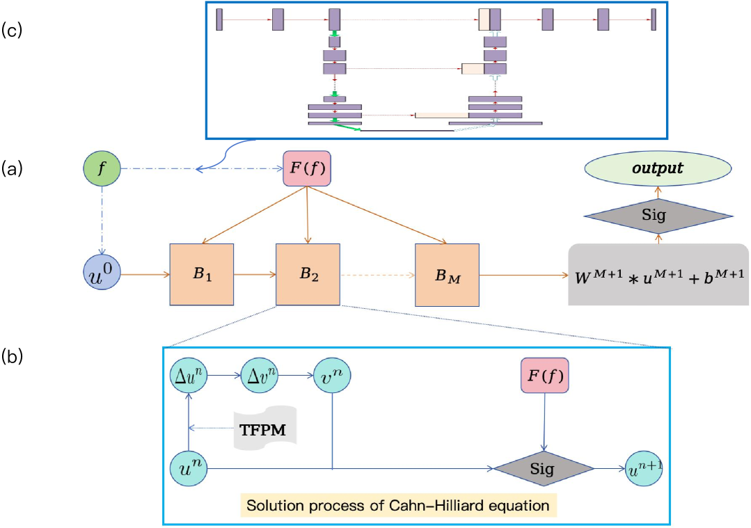
Assume is an image of size , then we approximate in Eq. (9) by a UNet class neural network specified by channel vector . We call the procedure a VM_TUNet block, denoted by ; see Figure 2(b) for an illustration with activation , where contains trainable parameters of . The input for includes the output of the previous block and . There are VM_TUNet blocks, is passed to all VM_TUNet blocks, and is passed through every VM_TUNet block sequentially. Denoting the -th VM_TUNet block by , and after , we add a convolution layer followed by a sigmoid function. Denote the kernel and bias in the last convolution layer by and , respectively, then we have VM_TUNet as the following formula
where we show the architecture of VM_TUNet in Figure 2.
PottsMGNet and Doublewell Nets derived from the Potts model and operator-splitting method give a clear explanation for the encode-decode type of neural network like UNet. However, the mathematical treatment and splitting treatment of PottsMGNet and Doublewell Net II (DN-II) are different from those of Doublewell Net I (DN-I) and VM_TUNet here. In addition, DN-I and VM_TUNet fix over time and assume is only a function of the input image liu2024double , but DN-II is not. In the meantime, VM_TUNet uses a higher-order Cahn-Hilliard equation model so that the sharp boundaries are well preserved during image segmentation, compared to the previous methods.
Accommodate periodic boundary conditions
Periodic boundary conditions are often considered in image segmentation liu2024double . Let and denote the two spatial directions by and . To accommodate the periodic boundary conditions, we replace Eq. (8) and Eq. (9) by
| (10) |
and
| (11) |
respectively.
Tailored finite point method
For in Eq. (10), we propose using the tailored finite point method (TFPM) method to compute it Han2010TailoredFP . Let
by linearizing we have
where and can be seen as slice constants yang2019image , then we can obtain
from
where on discretized mesh points.
Moreover, by solving
we have
For in Eq. (11), it is the laplacian of approximated by central difference, which is realized by convolution with
| (12) |
UNet class
The UNet class is designed to capture multiscale features of images, which features a symmetric encoder-decoder structure with skip connections to combine high-resolution features from the encoder with upsampled features from the decoder. For the resolution levels in the encoding and decoding parts, ordered from finest to coarsest, we represent their corresponding number of channels as a vector , where each element is a positive integer, and denotes the total number of resolution levels. For an image input with size , the structure of such a class is illustrated in Appendix A.1. Furthermore, UNet class has the advantage of light parameters compared to other deep learning methods such as Segment Anything model (SAM); see in Appendix A.2, so we prefer it for approximation of .
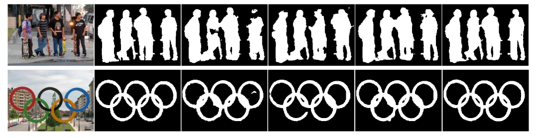
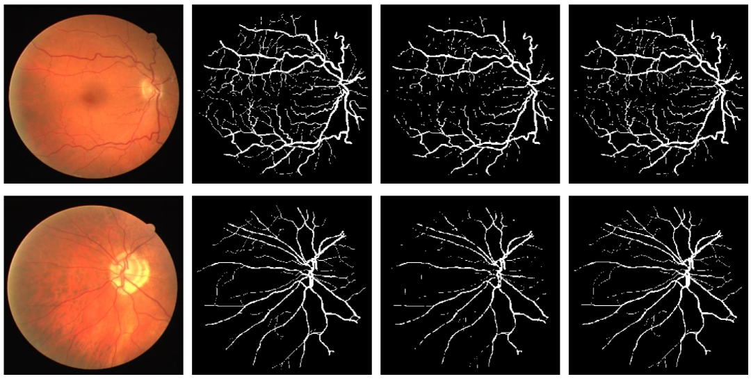
5 Experiments
In this section, we evaluate VM_TUNet on four semantic segmentation datasets: The Extended Complex Scene Saliency Dataset (ECSSD) 7182346 , the Retinal Images Vessel Tree Extraction Dataset (RITE) hu2013automated , HKU-IS LiYu15 and DUT-OMRON yang2013saliency . For ECSSD, we resize all images to the size 192256, using 800 images for training and 200 images for testing. For RITE, we resize all images to 256256, using 20 images for training and 20 images for testing. For HKU-IS, we resize all images to the size 256256, using 3000 images for training and 1447 images for testing. For DUT-OMRON, which contains 5168 high-quality natural images where each image contains one or more salient objects with varied and cluttered backgrounds, we resize all images to the size 256256, using 3500 images for training and 1668 images for testing. We train with Adam optimizer and 600 epochs for ECSSD and RITE, and 800 epochs for HKU-IS and DUT-OMRON. In the VM_TUNet model, without specification, the UNet architecture is employed with a channel configuration of . The model consists of 10 blocks, and the parameters are set as follows: , and , where these parameters in our model do not need to be manually tuned and will not have a greater impact on the results. We implement all numerical experiments on a single NVIDIA RTX 4090 GPU.
| ECSSD | RITE | HKU-IS | DUT-OMRON | |||||
| Accuracy | Dice score | Accuracy | Dice score | Accuracy | Dice score | Accuracy | Dice score | |
| UNet | 0.9220.003 | 0.8710.001 | 0.9300.004 | 0.6780.002 | 0.9040.003 | 0.8710.001 | 0.8810.001 | 0.8590.002 |
| UNet++ | 0.9250.004 | 0.8790.001 | 0.9370.005 | 0.6820.001 | 0.9080.001 | 0.8770.002 | 0.8890.002 | 0.8630.001 |
| DeepLabV3+ | 0.9280.003 | 0.8930.002 | 0.9420.002 | 0.6950.001 | 0.9230.002 | 0.8870.002 | 0.8920.001 | 0.8680.002 |
| DN-I | 0.9390.002 | 0.8820.001 | 0.9410.002 | 0.7020.002 | 0.9100.003 | 0.8810.001 | 0.8900.004 | 0.8710.001 |
| VM_TUNet | 0.9450.002 | 0.8950.002 | 0.9480.001 | 0.7130.002 | 0.9210.002 | 0.8900.001 | 0.9030.002 | 0.8780.002 |
We compare the proposed model with corresponding state-of-the-art image segmentation networks mainly including UNet ronneberger2015u , UNet++ Zhou2018UNetAN , DeepLabV3+ Chen_2018_ECCV and DN-I liu2024double ; see in Appendix B.4. In these models, the output is generated by passing the final layer through a sigmoid activation function, resulting in a tensor where each element falls within the range of . To convert this into a binary segmentation map, a threshold value is applied to the output matrix as
| (13) |
The similarity between the predicted output of the model and the provided ground truth mask is evaluated using two metrics, accuracy and the dice score:
| (14) |
and
| (15) |
where denotes the number of nonzero elements of a binary function and is the logic "and" operation.
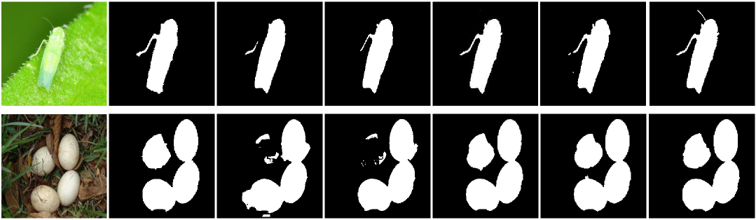
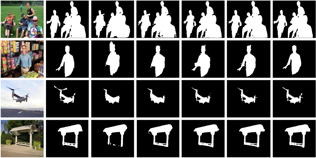
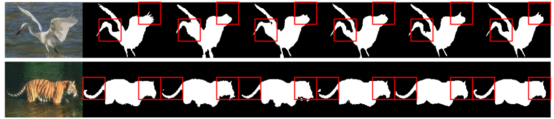
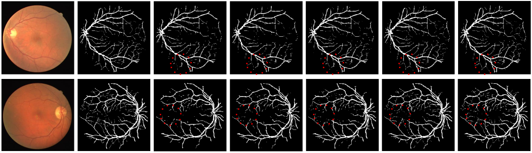
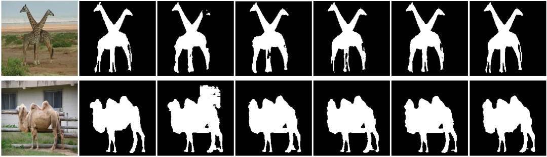
We present some selected segmentation results in Figures 3 and 4 and other results are shown in Appendix B.1, which are not the best or worst results of each dataset, respectively. The chosen images are intended to visually demonstrate the distinctions between the proposed approaches and currently available network architectures. The predictions generated by the proposed method closely align with the ground truth masks, whereas competing models exhibit inaccuracies, either by incorrectly segmenting certain objects or failing to capture specific regions entirely, especially at the borders. Particularly, for the cicada image segmentation task in the first row of Figure 3, whose ground truth does not have antennae, but our method makes it. To measure the complexity of different models, we present the outcome of loss, accuracy, and dice score in Table 1, and we can see that VM_TUNet outperforms other models.
6 Limitations
Experimental results show that while VM_TUNet performs well on datasets with fewer than 10,000 images and relatively involute backgrounds, its effectiveness decreases when applied to larger-scale datasets with over 10,000 images, especially those leaning toward the instance segmentation tasks, such as ADE Challenge on Scene Parsing Dataset (ADE20K), Common Objects in Context-Stuff Segmentation (COCO Stuff), DUT Salient Object Detection Dataset (DUT) and so on. This indicates that VM_TUNet still faces challenges in handling more complex scenes with dense and diverse object instances, which suggests the need for further improvements in model generalization, such as enhancing network architecture or incorporating stronger context modeling strategies.
7 Conclusion
In this paper, we propose VM_TUNet, an innovative approach that integrates the strengths of both traditional variational models and modern deep learning methods for image segmentation. By leveraging the Cahn-Hilliard equation and combining it with a deep learning framework based on the UNet architecture, we aim to overcome the limitations of conventional segmentation techniques. The key innovation in VM_TUNet lies in seamlessly incorporating variational principles, which provides interpretability and theoretical rigor, into the flexibility and accuracy of deep learning models. By using a data-driven operator, we eliminate the need for manual parameter tuning, which is a common challenge in traditional variational methods. Next, our use of the TFPM ensures that sharp boundaries are preserved during segmentation, even in complex images with intricate backgrounds. This method addresses the shortcomings of existing deep learning-based approaches by making the model more adaptable and capable of handling diverse input data without compromising segmentation quality. Our experimental results demonstrate that VM_TUNet outperforms existing segmentation models like UNet, UNet++, DeepLabV3+, and DN-I, which achieving higher accuracy and dice scores, particularly in challenging segmentation tasks with sharp boundaries.
The proposed VM_TUNet framework, which integrates the fourth-order Cahn-Hilliard equation with a UNet-based deep learning architecture, offers a promising direction for advancing image segmentation. Its strength lies in combining mathematical interpretability with data-driven adaptability. The use of the modified Cahn-Hilliard equation enhances boundary sharpness and structural consistency, which is particularly valuable for semantic segmentation tasks requiring precise delineation. Moreover, the data-driven formulation of the variational operator allows the model to generalize across diverse inputs, which suggests its potential application in multi-class and multi-instance settings. Additionally, its hybrid variational-deep learning approach provides a foundation for incorporating explicit structural priors or instance-aware constraints, making it a compelling candidate for future research in interpretable and robust segmentation models. However, VM_TUNet still struggles with complex scenes containing dense and diverse objects, indicating a need for better generalization through improved architecture or stronger context modeling.
References
- [1] V. Badrinarayanan, A. Kendall, and R. Cipolla. Segnet: A deep convolutional encoder-decoder architecture for image segmentation. IEEE Transactions on Pattern Analysis and Machine Intelligence, 39(12):2481–2495, 2017.
- [2] E. Bae, X.-C. Tai, and W. Zhu. Augmented Lagrangian method for an Euler’s elastica based segmentation model that promotes convex contours. Inverse Problems and Imaging, 11(1):1–23, 2017.
- [3] C. Bao, Q. Li, Z. Shen, C. Tai, L. Wu, and X. Xiang. Approximation analysis of convolutional neural networks. East Asian Journal on Applied Mathematics, 2023.
- [4] J. W. Cahn and J. E. Hilliard. Free energy of a nonuniform system. i. interfacial free energy. The Journal of Chemical Physics, 28(2):258–267, 1958.
- [5] V. Caselles, R. Kimmel, and G. Sapiro. Geodesic active contours. International Journal of Computer Vision, 22(1):61–79, 1997.
- [6] E. Celledoni, M. Ehrhardt, C. Etmann, R. Mclachlan, B. Owren, C.-B. Schonlieb, and F. Sherry. Structure-preserving deep learning. European Journal of Applied Mathematics, 32(5), 2021.
- [7] T. Chan and L. Vese. Active contours without edges. IEEE Transactions on Image Processing: a Publication of the IEEE Signal Processing Society, 10(2):266–277, 2001.
- [8] L.-C. Chen, Y. Zhu, G. Papandreou, F. Schroff, and H. Adam. Encoder-decoder with atrous separable convolution for semantic image segmentation. In Proceedings of the European Conference on Computer Vision (ECCV), September 2018.
- [9] X. Chen, B. M. Williams, S. R. Vallabhaneni, G. Czanner, R. Williams, and Y. Zheng. Learning active contour models for medical image segmentation. In 2019 IEEE/CVF Conference on Computer Vision and Pattern Recognition (CVPR). IEEE, 2019.
- [10] Y. Chen, W. Yu, and T. Pock. On learning optimized reaction diffusion processes for effective image restoration. In Proceedings of the IEEE Conference on Computer Vision and Pattern Recognition, pages 5261–5269, 2015.
- [11] D. Cheng, R. Liao, S. Fidler, and R. Urtasun. Darnet: Deep active ray network for building segmentation. In 2019 IEEE/CVF Conference on Computer Vision and Pattern Recognition (CVPR), pages 7423–7431. IEEE, 2019.
- [12] Z. Cui, T. Y. Pan, G. Yang, J. Zhao, and W. Wei. A trainable variational Chan-Vese network based on algorithm unfolding for image segmentation. Mathematical Foundations of Computing, pages 0–0, 2024.
- [13] H. Han and Z. Huang. Tailored finite point method for steady-state reaction-diffusion equations. Communications in Mathematical Sciences, 8:887–899, 2010.
- [14] Q. Hu, M. D. Abràmoff, and M. K. Garvin. Automated separation of binary overlapping trees in low-contrast color retinal images. In Medical Image Computing and Computer-Assisted Intervention–MICCAI 2013: 16th International Conference, Nagoya, Japan, September 22-26, 2013, Proceedings, Part II 16, pages 436–443. Springer, 2013.
- [15] P. Iakubovskii. Segmentation models pytorch. https://github.com/qubvel/segmentation_models.pytorch, 2019.
- [16] M. Kass, A. Witkin, and D. Terzopoulos. Snakes: Active contour models. International Journal of Computer Vision, 321(331):1987, 1988.
- [17] Y. Kim, S. Kim, T. Kim, and C. Kim. CNN-based semantic segmentation using level set loss. In 2019 IEEE Winter Conference on Applications of Computer Vision (WACV), pages 1752–1760. IEEE Computer Society, 2019.
- [18] A. Kirillov, E. Mintun, N. Ravi, H. Mao, C. Rolland, L. Gustafson, T. Xiao, S. Whitehead, A. C. Berg, W.-Y. Lo, et al. Segment anything. In Proceedings of the IEEE/CVF International Conference on Computer Vision, pages 4015–4026, 2023.
- [19] T. H. N. Le, K. G. Quach, K. Luu, C. N. Duong, and M. Savvides. Reformulating level sets as deep recurrent neural network approach to semantic segmentation. IEEE Transactions on Image Processing, 27(5):2393–2407, 2018.
- [20] G. Li and Y. Yu. Visual saliency based on multiscale deep features. In IEEE Conference on Computer Vision and Pattern Recognition (CVPR), pages 5455–5463, June 2015.
- [21] C. Liu, Z. Qiao, C. Li, and C.-B. Schönlieb. Inverse evolution layers: Physics-informed regularizers for image segmentation. SIAM Journal on Mathematics of Data Science, 7(1):55–85, 2025.
- [22] C. Liu, Z. Qiao, and Q. Zhang. Two-phase segmentation for intensity inhomogeneous images by the Allen–Cahn local binary fitting model. SIAM Journal on Scientific Computing, 44(1):B177–B196, 2022.
- [23] H. Liu, J. Liu, R. H. Chan, and X.-C. Tai. Double-well net for image segmentation. Multiscale Modeling & Simulation, 22(4):1449–1477, 2024.
- [24] H. Liu, X.-C. Tai, and C. Raymond. Connections between operator-splitting methods and deep neural networks with applications in image segmentation. Annals of Applied Mathematics, 39(4):406–428, 2023.
- [25] J. Long, E. Shelhamer, and T. Darrell. Fully convolutional networks for semantic segmentation. In 2015 IEEE Conference on Computer Vision and Pattern Recognition (CVPR), pages 3431–3440. IEEE Computer Society, 2015.
- [26] Y. Lu, A. Zhong, Q. Li, and B. Dong. Beyond finite layer neural networks: Bridging deep architectures and numerical differential equations. In International Conference on Machine Learning, pages 3276–3285. PMLR, 2018.
- [27] S. Lunz, O. Öktem, and C.-B. Schönlieb. Adversarial regularizers in inverse problems. Advances in Neural Information Processing Systems, 31, 2018.
- [28] D. Marcos, D. Tuia, B. Kellenberger, L. Zhang, M. Bai, R. Liao, and R. Urtasun. Learning deep structured active contours end-to-end. In Proceedings-2018 IEEE/CVF Conference on Computer Vision and Pattern Recognition, CVPR 2018, pages 8877–8885, 2018.
- [29] S. Minaee, Y. Y. Boykov, F. Porikli, A. J. Plaza, N. Kehtarnavaz, and D. Terzopoulos. Image segmentation using deep learning: A survey. IEEE Transactions on Pattern Analysis and Machine Intelligence, pages 1–1, 2021.
- [30] D. Mumford and J. Shah. Optimal approximations by piecewise smooth functions and associated variational problems. Communications on Pure and Applied Mathematics, 42(5):577–685, 1989.
- [31] O. Ronneberger, P. Fischer, and T. Brox. U-Net: Convolutional networks for biomedical image segmentation. In International Conference on Medical Image Computing and Computer-Assisted Intervention, pages 234–241. Springer, 2015.
- [32] L. Rosasco, E. De Vito, A. Caponnetto, M. Piana, and A. Verri. Are loss functions all the same? Neural Computation, 16(5):1063–1076, 2004.
- [33] L. Ruthotto and E. Haber. Deep neural networks motivated by partial differential equations. Journal of Mathematical Imaging and Vision, 62(3):352–364, 2020.
- [34] J. Shen, S. H. Kang, and T. F. Chan. Euler’s elastica and curvature-based inpainting. SIAM Journal on Applied Mathematics, 63(2):564–592, 2003.
- [35] J. Shi, Q. Yan, L. Xu, and J. Jia. Hierarchical image saliency detection on Extended CSSD. IEEE Transactions on Pattern Analysis and Machine Intelligence, 38(4):717–729, 2016.
- [36] X.-C. Tai, J. Hahn, and G. J. Chung. A fast algorithm for Euler’s elastica model using augmented Lagrangian method. SIAM Journal on Imaging Sciences, 4(1):313–344, 2011.
- [37] X.-C. Tai, H. Liu, and R. Chan. PottsMGNet: A mathematical explanation of encoder-decoder based neural networks. SIAM Journal on Imaging Sciences, 17(1):540–594, 2024.
- [38] L. A. Vese and T. F. Chan. A multiphase level set framework for image segmentation using the Mumford and Shah model. International Journal of Computer Vision, 50(3):271–293, 2002.
- [39] X. Wang, Z. Huang, and W. Zhu. Multi-phase segmentation using modified complex Cahn-Hilliard equations. Numerical Mathematics: Theory, Methods & Applications, 15(2), 2022.
- [40] Y. Wang, Z. Zhong, J. Zhao, S. Gong, Z. Pan, and W. Wei. PottsNN: A variational neural network based on Potts model for image segmentation. In Chinese Conference on Pattern Recognition and Computer Vision (PRCV), pages 142–156. Springer, 2024.
- [41] E. Weinan. A proposal on machine learning via dynamical systems. Communications in Mathematics and Statistics, 5(1):1–11, 2017.
- [42] C. Yang, L. Zhang, H. Lu, X. Ruan, and M.-H. Yang. Saliency detection via graph-based manifold ranking. In 2013 IEEE Conference on Computer Vision and Pattern Recognition, pages 3166–3173. IEEE, 2013.
- [43] W. Yang, Z. Huang, and W. Zhu. Image segmentation using the Cahn–Hilliard equation. Journal of Scientific Computing, 79(2):1057–1077, 2019.
- [44] K. Zhang, L. Zhang, H. Song, and W. Zhou. Active contours with selective local or global segmentation: A new formulation and level set method. Image and Vision Computing, 28:668–676, 2010.
- [45] Y. Zhang, Z. Shen, and R. Jiao. Segment anything model for medical image segmentation: Current applications and future directions. Computers in Biology and Medicine, page 108238, 2024.
- [46] Z. Zhou, M. M. R. Siddiquee, N. Tajbakhsh, and J. Liang. Unet++: A nested u-net architecture for medical image segmentation. Deep Learning in Medical Image Analysis and Multimodal Learning for Clinical Decision Support : 4th International Workshop, DLMIA 2018, and 8th International Workshop, ML-CDS 2018, held in conjunction with MICCAI 2018, Granada, Spain, S…, 11045:3–11, 2018.
- [47] W. Zhu, X. C. Tai, and T. Chan. Image segmentation using Euler’s elastica as the regularization. Journal of Scientific Computing, 57(2):414–438, 2013.
Appendix A UNet illustration
A.1 UNet type network
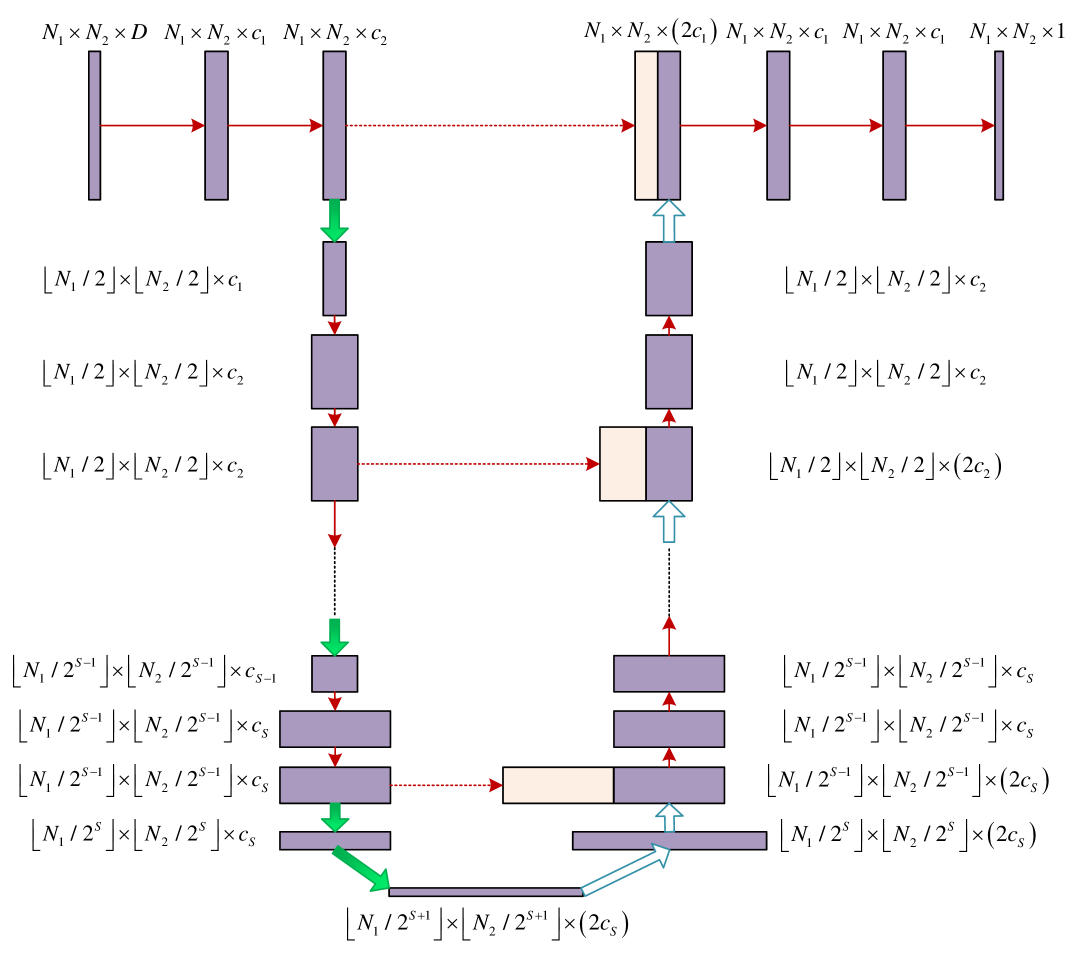
The architecture is designed to capture multiscale features of images: each resolution level corresponds to features of one scale. For the original UNet, it has . The general UNet type architecture used here for image segmentation is inspired by the original UNet, which features a symmetric encoder-decoder design with skip connections that bridge high-resolution features from the contracting path to the expanding path. This structure enables precise localization while maintaining semantic context, which makes UNet especially effective in segmentation tasks with limited training data. The architecture follows this foundational UNet paradigm, which maintains the characteristic downsampling and upsampling paths connected via skip connections. This modification enhances the representational robustness of the latent features, encouraging a more distinct and stable embedding of segmentation-relevant structures. While still falling under the umbrella of "UNet-like" architectures, VM_TUNet extends the traditional UNet by embedding a task-driven regularization objective into its core, which contributes to improved generalization and sharper segmentation boundaries—especially in challenging or ambiguous regions of the input.
A.2 Lightweight architecture
In this paper, we only modified the PDE equation and calculation method, and did not change the original architecture of UNet. The number of parameters in our model is not much different from that in DN-I, and we fully utilize the advantage of the UNet network architecture being lightweight compared to the Segment Anything model (SAM) and so on. The comparison of parameters of various deep learning methods in image segmentation is shown in Table 2.
| Number of parameters on ECSSD | ||||||
| DN-I | VM_TUNet | UNet | UNet++ | DeepLabV3+ | TransUNet | SAM |
| 7.7M | 7.8M | 31.0M | 35.0M | 40.0M | 105.0M | > 600.0M |
In certain tasks, especially those involving limited computational resources or small-scale datasets, it is often preferable to use lightweight architectures like UNet over large-scale models such as the SAM. UNet offers a highly efficient encoder-decoder structure with significantly fewer parameters, making it ideal for applications like medical image segmentation or embedded systems where inference speed and memory usage are critical. While SAM demonstrates strong generalization and zero-shot capabilities, its massive size and resource demands make it less suitable for scenarios requiring fast, cost-effective deployment or fine-tuning on small domain-specific datasets. Another advantage of UNet is that it does not require pretraining on large-scale datasets, unlike many modern deep learning models that rely on extensive pretraining. UNet is designed to perform well even when trained from scratch on relatively small datasets, thanks to its symmetric architecture and skip connections that preserve spatial information effectively. This makes it particularly suitable for domains like biomedical imaging, where annotated data is scarce and domain-specific features differ significantly from natural images.
Appendix B Additional experimental results
B.1 Experiments on other datasets
ECSSD
ECSSD is a semantic segmentation data set containing 1000 images with complex backgrounds and manually labeled masks. The partial results of ECSSD is shown in Figure 6.
RITE
RITE is a dataset for the segmentation and classification of arteries and veins on the retinal fundus containing 40 images. The partial results of RITE is shown in Figure 7.
HKU-IS
HKU-IS is a visual saliency prediction dataset which contains 4447 challenging images, most of which have either low contrast or multiple salient objects. The partial results of HKU-IS is shown in Figure 8.
B.2 Comparative trial: Replacement of UNet with a simple CNN
To examine whether the performance gain of VM_TUNet is due to the specific architecture of UNet or simply to its parameter scale, we conduct an ablation study by replacing the UNet-based approximation of with a plain convolutional neural network–FlatCNN. The FlatCNN consists of a deep stack of 2D convolutional layers followed by batch normalizations and ReLU activations, without skip connections, downsampling and upsampling modules. The total number of parameters is controlled to be approximately 30 million, comparable to the UNet used in the main experiments.
The architecture follows the following form: where is the number of convolutional blocks, adjusted to match the UNet’s parameter budget, whose architecture overview is shown in Table 3.
| Hierarchy | Layer | Number of output channel | Convolution kernel size | Activation & Normalization |
|---|---|---|---|---|
| 1 | Conv2D | 128 | 33 | ReLU+BN |
| 2-5 | Conv2D4 | 256 | 33 | ReLU+BN |
| 6-10 | Conv2D5 | 512 | 33 | ReLU+BN |
| 11 | Conv2D | 256 | 33 | ReLU+BN |
| 12 | Conv2D | 128 | 33 | ReLU+BN |
| 13 | Conv2D | 1 | 11 | Sigmoid |
At the same time, we also use ResNet50 and DenseNet264 whose number of parameters is similar to UNet to approximate and we have some selected segmentation results in Figure 9 and Table 4 under the same experimental conditions where the result shows that UNet performs better than simple CNNs.
| ECSSD | |||
| Accuracy | Dice score | ||
| ResNet50 | 0.8230.003 | 0.8010.001 | |
| DenseNet | 0.8550.001 | 0.8310.001 | |
| FlatCNN | 0.8880.001 | 0.8720.002 | |
| UNet | 0.9490.002 | 0.9060.002 | |
B.3 Comparative trial: Replacement of TFPM with finite difference method
For Eq. (10) and Eq. (11), we just use simple finite difference method (FDM) without TFPM to get the procedure where and are only approximated by central difference, which are realized by convolution and by Eq. (12). The computational schemes are
| (16) |
and
| (17) |
respectively. Some selected segmentation results are shown in Figure 10 under the same experimental conditions where the result obviously shows that TFPM performs better than FDM.
B.4 Reproducibility of results of other methods
The PyTorch code of DN-I is available at https://github.com/liuhaozm/Double-well-Net. In our experiments, UNet, UNet++ and DeepLabV3+ are implemented by using the Segmentation Models PyTorch package [15].
Appendix C Mathematical background
C.1 Chan-Vese model
The Chan-Vese segmentation algorithm is designed to segment objects without clearly defined boundaries. This algorithm is based on level sets that are evolved iteratively to minimize an energy, which is defined by weighted values corresponding to the sum of differences intensity from the average value outside the segmented region, the sum of differences from the average value inside the segmented region, and a term which is dependent on the length of the boundary of the segmented region. This algorithm was first proposed by Tony Chan and Luminita Vese, which is based on the Mumford–Shah functional and aims to segment an image by finding a contour that best separates the image into regions of approximately constant intensity.
It seeks to minimize the following energy functional
where is the input image; are average intensities inside and outside the contour; are positive weighting parameters; and is the contour boundary.
To handle topology changes, like contour splitting, the contour is represented implicitly using a level set function such that
where is the image domain. Using the Heaviside function , the energy can be rewritten in the level set form
where is the Heaviside function and is the Dirac delta approximation.
At each iteration, the optimal values of and (region averages) are
To minimize the energy, the level set function evolves according to the Euler–Lagrange equation, leading to the following PDE
where the first term is a regularization term (curvature) and the second and third terms are data fidelity forces, pushing the contour to regions where is closer to or .
The Dirac delta function is approximated as
and the Heaviside function is approximated as
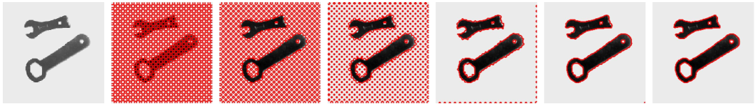
In [7], authors proposed a numerical algorithm using finite differences to solve this problem. In the Chan-Vese image segmentation algorithm, the contour appears dense and scattered at the beginning because of the initialization of the level set function. Typically, the level set function is initialized with a shape (like a circle or square) that defines the starting contour. Around the zero level set, there may be many values close to zero due to discretization and numerical approximation, which can lead to the appearance of multiple contour lines when visualized. Additionally, some implementations deliberately initialize multiple contours to help the algorithm explore the image structure more effectively. As the algorithm iterates, these contours evolve and gradually merge into a single, smooth boundary that accurately segments the object of interest.
C.2 Cahn-Hilliard equation
The Cahn-Hilliard equation was originally proposed by Cahn and Hilliard and describes the phase separation that occurs when a mixture of two substances is quenched into an unstable state [4]. The Cahn-Hilliard equation is the gradient flow of the generalized Ginzberg Landau proper energy functional under the norm. Van der Waals first proposed the generalized Ginzberg-Landau free energy functional, which accurately describes the mixing energy of two substances
where represents the concentration of one of the species, the concentration of the other species is , is the double well function or Lyapunov functional and the parameter controls the interface between the two metals.
The space is the zero-mean dual subspace of , that is, for any given holds if and only if . Define the inner product on as
where , . The Gateaux derivative of is
Thereby,
that is, . The directional derivative of at with respect to direction is , along direction , the directional derivative is negative and is the largest. This direction is called the direction of fastest descent, so the gradient flow is