Formation Maneuver Control Based on the Augmented Laplacian Method
Abstract
This paper proposes a novel formation maneuver control method for both 2-D and 3-D space, which enables the formation to translate, scale, and rotate with arbitrary orientation. The core innovation is the novel design of weights in the proposed augmented Laplacian matrix. Instead of using scalars, we represent weights as matrices, which are designed based on a specified rotation axis and allow the formation to perform rotation in 3-D space. To further improve the flexibility and scalability of the formation, the rotational axis adjustment approach and dynamic agent reconfiguration method are developed, allowing formations to rotate around arbitrary axes in 3-D space and new agents to join the formation. Theoretical analysis is provided to show that the proposed approach preserves the original configuration of the formation. The proposed method maintains the advantages of the complex Laplacian-based method, including reduced neighbor requirements and no reliance on generic or convex nominal configurations, while achieving arbitrary orientation rotations via a more simplified implementation. Simulations in both 2-D and 3-D space validate the effectiveness of the proposed method.
I Introduction
In recent years, formation control of multi-agent systems has gained significant attention due to its wide range of applications in various fields, such as drone swarms[1], AUV formations [2], robotic cooperation[3], etc. While formation shape control remains essential for coordinated tasks, most scenarios increasingly require dynamic adaptability. This promotes the shift from formation shape control to formation maneuver control, which enables formations to perform continuous shape variation. Formation maneuver control faces the new challenge of maintaining invariant geometric features during the maneuver process.
Although conventional consensus-based formation control methods are capable of tracking time-varying formations, they usually require agents to have explicit knowledge of target positions[4, 5]. Nevertheless, in most cases, agents are mainly restricted to gathering information from their neighboring agents rather than having access to global information [6]. To deal with this issue, displacement-based[7, 8], distance-based[9], and bearing-based methods[10, 11] utilize the information from neighboring agents. They define target formations through invariant constraints on inter-agent displacements, distances, and bearings. Ren et al. [7, 8] proposed displacement-based method which successfully tracks time-varying formation translation yet encounters difficulties when dealing with time-varying scaling and rotation. De Marina et al. [9] put forward a distance-based method that is capable of handling time-varying formation translation and rotation while being ineffective in managing scaling. Zhao et al. [10, 11] introduced bearing-based method which can accommodate time-varying formation translation and scaling while being unable to execute formation rotation.
Recent researches have improved formation maneuverability by introducing advanced constraints, such as similarity-based rigidity constraints, complex Laplacian, equilibrium stress matrices, and barycentric coordinates. The formation maneuver control method[12] based on similarity-based rigidity constraints effectively enables formation shape variation under translation, rotation, and scaling, but the inherent rigidity may pose challenges in terms of flexibility for reconfiguration. The complex Laplacian approach[13, 14, 15, 16] enables formation shape variation under translation, rotation, and scaling. Because of the property of complex numbers, this method is restricted to 2-D space. Xu et al. [17] extended the complex Laplacian-based method to 3-D space by introducing an additional dimension. To achieve rotation with any orientation in 3-D space, the method requires constructing three constant nominal configurations, which leads to high complexity and redundancy. In contrast, formation maneuver control methods based on equilibrium stress matrices[18, 19, 20, 21] and barycentric coordinates[22, 23] support any-dimensional formation shape variation. However, these methods still have the following two issues. First, followers require at least neighbors in -dimensional space. Second, nominal configurations must satisfy generic or rigid conditions to construct an invertible follower-follower matrix, which ensures unique and localizable formations.
In this paper, we present a novel formation maneuver control method based on the augmented Laplacian matrix. The proposed approach enables formations to simultaneously execute translational, rotational, and scaling maneuvers in both 2-D and 3-D space. Compared with existing methods, our main contributions are as follows:
-
•
Instead of scalar values, the weights of inter-agent constraints are represented as matrices, which enables the formation to rotate about the given rotation axis.
-
•
To achieve arbitrary orientation rotations of the formation, we propose a dynamic rotation axis adjustment approach. We also develop a dynamic agent reconfiguration method that allows seamless integration of new agents into the formation. It is proved that both methods preserve the invariance of formation’s configuration.
-
•
We establish a theoretical connection between the proposed method and existing complex Laplacian method, thereby showing that the complex Laplacian method is actually a special case of our method.
The rest of this paper is organized as follows. Section II presents some preliminaries and the objectives of this paper. Section III proposes the augmented Laplacian matrix, and control protocols for both leaders and followers. Further, we give methods for adjusting the rotation axis of formation and dynamic agent reconfiguration. Section IV reveals the relationship between the proposed method and the 2-D complex Laplacian method. Simulation results are presented in Section V to validate the effectiveness of our proposed method. Lastly, the conclusion is given in Section VI.
II Preliminaries and Problem Formulation
II-A Notations
Let be the set of real numbers, and be the set of complex numbers. is the transpose of the real matrix . Consider a multi-agent system with agents in , where and . Let be the position of the -th agent, be the nominal position and be the target position at time . Denote the interaction graph among the agents as , where and are the sets of agents and edges, respectively. This paper only considers 2-rooted graphs, i.e., there is a subset of two agents, and every other agent is 2-reachable from this subset [13].
Denote as a formation of agents, where is the interaction graph and is the configuration of the formation. Similarly, let and be the target formation and nominal formation, where and . A nominal configuration is called generic if the coordinates do not satisfy any nontrivial algebraic equation with integer coefficients [17]. The centroid of the nominal formation is defined as
| (1) |
Let and be the sets of followers and leaders. Let and be the configurations of followers and leaders, respectively. Similarly, let , and , be the target configuration and nominal configuration.
Let be the axis of rotation in 3-D space, and be the skew-symmetric matrix of vector . Let be the set of neighbors of agent . Let be an identity matrix of dimension , and be the all-one vector of dimension . Let be the Kronecker product.
II-B Invariant Constraints
A main challenge in formation maneuver control lies in the design of constraints, which maintain invariance under formation transformations. Specifically, the constraints are realized through the design of edge weights in the formation’s interaction graph. For instance, the constraint proposed in [11] maintains translation and scaling invariance through bearing-based weights , while the constraint in [18] extends the invariance to affine transformations.
A general form of constraints is formulated as
| (2) |
where are the weights on the edges . Then, the constraint matrix is defined as
| (3) |
The shape of the matrix differs among different methods. For instance, in the complex Laplacian methods [13, 14, 15, 16], , while in the methods based on equilibrium stress matrices [18, 19, 20, 21], . In general, (2) can be written in the matrix form as
| (4) |
Then, given a configuration , an immediate question is how to generate weights under constraints (2). Specifically, the work [13] addressed this by decomposing the problem into cases where agents have exactly two neighbors and those with more than two neighbors. First, for agent with two neighbors, , the weights are designed as
| (5) |
Second, for agent with more than two neighbors, where , the weights are constructed via
| (\theparentequation-a) | |||
| (\theparentequation-b) | |||
which, in essence, converts the problem into combinations of two-neighbor cases.
The constraint matrix, , is partitioned into follower-leader blocks as
| (7) |
where and describe the follower-follower and leader-leader blocks, respectively. The cross blocks and describe leader-follower interactions.
Definition 1.
A nominal formation is termed localizable if the follower-follower matrix is non-singular.
When the formation configuration is at nominal configuration , (4) decomposes into follower-leader blocks as
| (8) |
which further implies . Given the leaders’ nominal configuration , non-singularity of the matrix guarantees the existence of a unique solution for the followers’ configuration . Specifically,
| (9) |
Assumption 1.
The nominal formation is localizable, i.e., the matrix is non-singular.
In Sec. III, we will show the rationality of this assumption.
II-C Target Formation and Objectives
The translation and scaling parameters are denoted by and . In addition, denote as the rotation matrix about axis . Let be the rotation angle. By Rodrigues’ rotation formula, the rotation matrix is expressed as
| (10) |
Subsequently, according to [17], the time-varying target configuration is defined similarly based on the nominal configuration as
| (11) |
where is the translation term and is the scaling and rotation term.
Definition 2.
For a nominal formation , a target formation is termed similar to , if there is a specific rotation axis , such that the constraint matrix generated by the nominal formation satisfies
| (12) |
During formation maneuvers, the time-varying target formation should remain similar to for all time, i.e., .
Assumption 2.
Only leaders get access to the target positions, which means only leaders know the time-varying parameters in (11). Followers only know the relative positions and velocities of their neighbors.
Under Assumption 1 and Assumption 2, and leveraging (11) and (12), the target configurations of the leader and follower groups are written as
Then, the objectives of this paper are as follows.
-
•
Design a constraint matrix to ensure that the target formation configuration satisfies (12) for all time during formation maneuvers.
-
•
Design control protocols for the leaders and followers such that
(\theparentequation-a) (\theparentequation-b) -
•
Propose a method that enables the formation to adjust its rotation axis at any time to rotate with any orientations in 3-D space.
-
•
Develop a method enabling the real-time and seamless integration of new agents into the formation.
III Methodology
III-A Augmented Laplacian Matrix
In 3-D formation maneuver control, a fundamental challenge is achieving arbitrary formation rotations. Existing methods often lack systematic and straightforward solutions for this problem. To address this gap, we propose the augmented Laplacian matrix, where weights are matrices in rather than scalars.
Definition 3.
Given rotation axis , the augmented Laplacian matrix is expressed in the form of (3), and each weight is defined by
| (14) |
where coefficients .
As shown in (5) and (6), regardless of the number of neighbors agent has, the problem can be split into combinations of two-neighbor cases. Therefore, assuming that agents are the neighbors of agent , by (2), (5) and (6), we have
| (15) |
There are six unknowns () and three equations in (III-A). By the rank-nullity theorem, a non-trivial solution exists if and only if the coefficient matrix has rank less than three. Under Assumption 1, feasible weight matrices can always be constructed to satisfy (2).
Theorem 1.
Given rotation axis , the weight defined in (14) commutes with the rotation matrix , i.e.,
Proof.
Theorem 2.
Proof.
For the nominal formation , the constraints (2) are expressed as
| (16) |
First, for the translation term in (11), we have
Second, for the scaling and rotation term , we have
For each row, by Theorem 1, commutes with
Thus, we obtain
Therefore, given the augmented Laplacian matrix with entries in the form of (14), the target formation is similar to the nominal formation for all time.
∎
III-B Control Protocols
Consider that each agent is modeled as a single-integrator
| (17) |
where is the control protocol to be designed. Subsequently, we will present the specific forms for leaders and followers respectively.
Control Protocol for the Leaders. According to [17], a feasible control protocol for the leaders is obtained as
| (18) |
where is the control input, is the hyperbolic tangent function, and , , are the target velocities.
Lemma 1 (Lemma 3 [17]).
The leaders group achieves their control objective (\theparentequation-a) under control protocol (18).
Control Protocol for the Followers. Under Assumption 1, the followers can utilize constant weights in and to achieve formation maneuver control without knowing the time-varying parameters in (11). The distributed control protocol for followers is given by
| (19) |
where represents the sum of weights for agent ’s neighbors, and is a positive control gain parameter. In matrix form, (19) is expressed as
| (20) |
Lemma 2.
The followers group achieves their control objective (\theparentequation-b) under control protocol (20).
Proof.
Let represent the tracking error for followers, which is defined by
Differentiating this equation gives
Consider a Lyapunov function
The time derivative of is
Since for , the desired conclusion holds.
∎
III-C Rotation Axis Adjustment
Since the augmented Laplacian matrix is related to , the proposed augmented Laplacian method confines the formation to rotate around a given axis . Thus, a natural question is how to enable the formation to rotate with any orientations in 3-D space. To address this issue, we introduce a method for adjusting the rotation axis during the formation maneuver, while maintaining the invariance of the formation geometry.
First, at time , the formation reaches the target configuration, i.e., . At this specific time , the rotation axis is adjusted from to . Next, based on the current formation and rotation axis , the augmented Laplacian matrix must be reconstructed. Finally, in accordance with (11), the target configuration for the subsequent formation maneuver is expressed as
| (21) |
where and .
Theorem 3.
After adjusting the rotation axis to , the new target formation is still similar to the nominal formation .
Proof.
From (21), we have
Then, (21) is transformed to
where is treated as , is treated as and is treated as . According to Definition 2, the new target formation is still similar to the nominal formation . ∎
III-D Dynamic Agent Reconfiguration
In practical cases, the integration of new agents into a formation is widely adopted, highlighting the significance of a scalable formation maneuver control method. In this subsection, we propose a method that allows new agents to seamlessly join the formation at any time for dynamic reconfiguration.
Specifically, the integration of a new agent into the formation involves the following steps. Initially, during the original formation maneuver, the new agent identifies its time-varying joining position. Upon determining this position, the agent utilizes the control law (18) to reach its target position. Once the new agent arrives at the designated position, the augmented Laplacian matrix is reconstructed to accommodate the new agent while preserving the configuration of the original part. Ultimately, the integrated agent employs the distributed follower control protocol to maintain its relative position within the desired formation during subsequent maneuvers.
Theorem 4.
After a new agent joins the formation, the method proposed above maintains the configuration of the original part, i.e., , where is the configuration after the addition of a new agent .
Proof.
After the integration of the new agent, the positions of all agents in the formation are represented by
| (22) |
where is the position of the added agent.
Then, the reconstructed augmented Laplacian matrix is presented in , where satisfies , represents the extended matrix of the original augmented Laplacian matrix , with the specific form as
and represents the augmented Laplacian matrix exclusively concerning the added agent and its neighbors. By constraints (2), considering the original configuration and the new agent, we have
| (23) |
Hence, must satisfy . It follows that , which further implies that . Thus, we have
Since the leaders’ positions remain invariant during the integration of the new agent, i.e., , it is concluded that the positions of the original followers in the formation also remain unchanged:
Therefore, the integration of new agents maintains the invariance of the original formation configuration. ∎
IV Relationships with 2-D Complex Laplacian Method
In this section, we show that the 3-D formation maneuver control method based on the augmented Laplacian matrix proposed in this paper can be treated as an extension of the 2-D complex Laplacian method [11, 15].
In the complex Laplacian approach, the complex positions and weights are expressed as and , respectively, where and is the imaginary unit with . For any position , the weights acting on are expressed as
| (24) |
In 2-D plane rotations, all transformations occur around the Z-axis, which allows the 2-D complex Laplacian method to be considered as a special case of the proposed augmented Laplacian approach under rotations about the axis . To align with the complex Laplacian method, we adjust the order of coefficients in equation (14)
| (25) |
Weights constructed in (IV) have the same property as complex weights. First, for any position in 2-D space, the action of weights on is
| (26) |
which is equivalent to the action (24) in complex domain. Additionally, by Theorem 1, weights constructed in the proposed augmented Laplacian method also commute with rotation matrices , which is trivial for the complex Laplacian method due to the property of scalars.
Therefore, our proposed method is also available in 2-D space. Let be the rotation matrix around the Z-axis. Then the target configuration is expressed as follows,
| (27) |
By Theorem 2, the target formation is similar to its nominal formation, i.e., . Therefore, the complex Laplacian method is equivalent to the method proposed in this paper in 2-D space, both in terms of the construction of weights and the representation of the target formation.
Notably, the key difference between the 2-D and 3-D scenarios lies in the form of the weights . For 2-D cases, the construction of weights is simplified to the expression in (IV). In spite of this, the theorems and control protocols proposed in Sec. III can be directly applied to 2-D cases without any modification.
V Simulation
We will present two simulation examples in both 2-D and 3-D space. The multi-agent systems in 2-D and 3-D space both consist of three followers and two leaders shown in Fig. 1 and Fig. 3, where the trajectories of the followers and leaders are marked in blue and red, and the trajectory of the new agent in 3-D simulation is marked in green. In Fig. 1 and Fig. 3, the formations connected by gray lines are non-target formations, while the formations connected by green lines are target formations. The red arrows in Fig. 3 represent the rotation axis.
V-A Analysis of 2-D Simulation Results
In the 2-D simulation, the nominal configuration is designed as
with the positions of agents represented in 3-D to directly use the 3-D method proposed in this paper.
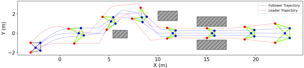
In this simulation, we verify the feasibility of our method in 2-D space. As shown in Fig. 1, the 2-D formation can freely translate, scale and rotate to avoid obstacles. As shown in Fig. 2, the control protocols we designed ensure that the formation quickly converges to the target formation.

V-B Analysis of 3-D Simulation Results
In the 3-D simulation, the nominal configuration is designed as
Note that since there are only two leaders, the line connecting them must not be parallel to the axis of rotation.
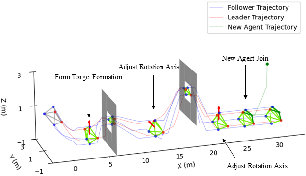
In this simulation, as shown in Fig. 3, we not only verify that, based on the proposed control method, the formation is capable of translating, scaling and rotating around any axis in 3-D space, but also show that it is possible for the formation to realize reconfiguration.
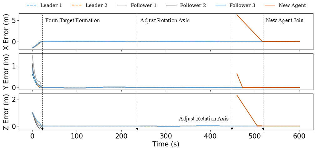
Fig. 4 presents that tracking errors in each axis for both the agents in the formation and the new agent converge to zero quickly, which shows the effectiveness of our proposed control protocols.
Overall, the simulations demonstrate the effectiveness of our proposed formation maneuver control method in both 2-D and 3-D space. A key advantage of our method is the capacity to perform arbitrary rotations, which allows for complex maneuvers. Furthermore, our method achieves formation maneuverability with only two leaders in 3-D space. Additionally, the proposed method does not require convex or generic configurations, providing greater flexibility in formation design. These features collectively contribute to the robustness and versatility of our formation maneuver control method.
VI Conclusions
This work introduces a general formation maneuver control method in both 2D and 3D space based on a novel constraint called augmented Laplacian matrix. The proposed method enables the formation to translate, scale, and rotate with any orientations. Moreover, for practical applications, we propose the dynamic agent reconfiguration approach, which allows new agents to join the formation, while maintaining the original configuration. Eventually, we give the relationships between our proposed method and the 2-D complex Laplacian method, which can be considered as a special case of our approach.
References
- [1] Mu, Lan, et al. “Motion behaviour based communication range estimation of adversarial drone swarms.” IEEE Transactions on Network Science and Engineering, (2025).
- [2] Xu, Jian, Shunxing Wei, and Liangang Yin. “Novel distributed energy-saving control method for multi-AUV formation under long time-varying delays and clock errors.” Ocean Engineering, 317 (2025): 119993.
- [3] Dabass, Vandana, and Suman Sangwan. “Strategic allocation: exploring optimization techniques in multi-robot systems.” International Journal of Intelligent Robotics and Applications, (2025): 1-23.
- [4] Amirkhani, Abdollah, and Amir Hossein Barshooi. “Consensus in multi-agent systems: a review.” Artificial Intelligence Review, 55.5 (2022): 3897-3935.
- [5] Gulzar, Muhammad Majid, et al. “Multi-agent cooperative control consensus: A comparative review.” Electronics, 7.2 (2018): 22.
- [6] Liu, Yefeng, et al. “A survey of multi-agent systems on distributed formation control.” Unmanned Systems, 12.05 (2024): 913-926.
- [7] Ren, Wei. “Multi-vehicle consensus with a time-varying reference state.” Systems & Control Letters, 56.7-8 (2007): 474-483.
- [8] Ren, Wei, and Randal W. Beard. “Consensus algorithms for double-integrator dynamics.” Distributed Consensus in Multi-vehicle Cooperative Control: Theory and Applications, (2008): 77-104.
- [9] De Marina, Hector Garcia, Bayu Jayawardhana, and Ming Cao. “Distributed rotational and translational maneuvering of rigid formations and their applications.” IEEE Transactions on Robotics, 32.3 (2016): 684-697.
- [10] Zhao, Shiyu, and Daniel Zelazo. “Bearing rigidity and almost global bearing-only formation stabilization.” IEEE Transactions on Automatic Control, 61.5 (2015): 1255-1268.
- [11] Zhao, Shiyu, and Daniel Zelazo. “Translational and scaling formation maneuver control via a bearing-based approach.” IEEE Transactions on Control of Network Systems, 4.3 (2015): 429-438.
- [12] Huang, Yunchang and Dai, Shi-Lu, “Similarity-based rigidity formation maneuver control of underactuated surface vehicles over directed graphs.” IEEE Transactions on Control of Network Systems, 12.1 (2025): 461-473.
- [13] Lin, Zhiyun, et al. “Distributed formation control of multi-agent systems using complex Laplacian.” IEEE Transactions on Automatic Control, 59.7 (2014): 1765-1777.
- [14] Fang, Xu, Lihua Xie, and Xiaolei Li. “Distributed localization in dynamic networks via complex laplacian.” Automatica, 151 (2023): 110915.
- [15] de Marina, Hector Garcia. “Distributed formation maneuver control by manipulating the complex Laplacian.” Automatica, 132 (2021): 109813.
- [16] Han, Zhimin, et al. “Formation control with size scaling via a complex Laplacian-based approach.” IEEE transactions on cybernetics, 46.10 (2015): 2348-2359.
- [17] Fang, Xu, and Lihua Xie. “Distributed formation maneuver control using complex laplacian.” IEEE Transactions on Automatic Control, 69.3 (2023): 1850-1857.
- [18] Zhao, Shiyu. “Affine formation maneuver control of multiagent systems.” IEEE Transactions on Automatic Control, 63.12 (2018): 4140-4155.
- [19] Chen, Liangming, et al. “Distributed leader–follower affine formation maneuver control for high-order multiagent systems.” IEEE Transactions on Automatic Control, 65.11 (2020): 4941-4948.
- [20] Xu, Yang, et al. “Affine formation maneuver control of high-order multi-agent systems over directed networks.” Automatica, 118 (2020): 109004.
- [21] Zhu, Cheng, et al. “Distributed affine formation maneuver control of autonomous surface vehicles with event-triggered data transmission mechanism.” IEEE Transactions on Control Systems Technology, 31.3 (2022): 1006-1017.
- [22] Xu, Yang, DeLin Luo, and HaiBin Duan. “Distributed planar formation maneuvering of leader-follower networked systems via a barycentric coordinate-based approach.” Science China Technological Sciences, 64.8 (2021): 1705-1718.
- [23] Fang, Xu, Xiaolei Li, and Lihua Xie. “Distributed formation maneuver control of multiagent systems over directed graphs.” IEEE Transactions on Cybernetics, 52.8 (2021): 8201-8212.