TESS Data Mining and UVES Spectral Analysis of CP Stars

Abstract

Photometric data from TESS were analyzed to obtain the light curve, confirming that the orbital period ($P=11.307\pm 0.005$ days) remains constant. A wavelet analysis was applied to detect temporal anomalies. The photometric effective temperature of HD 72968 was estimated through colorimetry, comparing it with main-sequence stars. UVES spectra were analyzed, Doppler-corrected, and normalized using Chebyshev functions. A theoretical spectral grid generated with SPECTRUM and ATLAS9 was fitted using the chi-squared method. A comparison with UVES-ESO spectra refined the temperature estimate of HD 72968. The analysis of the spectral energy distribution (SED) enabled the derivation of stellar parameters, validating the models employed. These results provide new insights into the atmosphere and variability of HD 72968 and motivate further spectral studies for improved stellar modeling.

Se analizaron datos fotométricos de TESS para obtener la curva de luz, confirmando que el periódo orbital ($P=11.307\pm 0.005$ días) es constante. Se aplicó un análisis wavelet para detectar anomalías temporales. La temperatura efectiva fotométrica de HD 72968 se estimó por colorimetría, comparándola con estrellas de la secuencia principal. Se analizaron espectros UVES corregidos por Doppler y normalizados con funciones de Chebyshev. Una cuadrícula espectral teórica generada con SPECTRUM y ATLAS9 fue ajustada mediante método chi-cuadrado. El contraste con espectros UVES-ESO refinó la temperatura de la estrella HD 72968. El análisis de la distribución espectral de energía (SED) permitió derivar parámetros estelares, validando los modelos empleados. Los resultados aportan nuevas perspectivas sobre la atmósfera y variabilidad de HD 72968, y motivan estudios espectrales más detallados.

TESS UVES spectroscopy chemically peculiar stars spectral energy distribution stellar parameters

0.1 INTRODUCTION

Chemically peculiar (CP) stars were first identified and classified by Maury & Pickering (1897) during spectral classification efforts in the Henry Draper Memorial project at Harvard, specifically describing the notable spectral characteristics of $\alpha^{2}$ CVn (Cor Caroli). Later, Morgan (1931) focused on Ap stars and certain manganese stars, correlating abundance anomalies with ionization temperatures and defining five groups of peculiar A stars (Morgan, 1933).

Additionally, Babcock (1958) conducted a comprehensive study of 70 A-type stars with sharp or ultra-sharp lines, including subdwarfs, M giants, and S-type stars, recognizing magnetic variability as a general feature. CP stars exhibit an excess abundance of elements with $\rm{Z>26}$, sometimes exceeding two orders of magnitude compared to the solar abundance. The strong magnetic fields of these stars have been linked to these abundance anomalies, with typical horizontal field strengths reaching thousands of gauss (Jaschek & Jaschek, 1968). Diffusion processes in A-type stars (Michaud, 1970) suggest that CP stars make up  10% of early B to F main-sequence stars. Preston (1974) later proposed a four-group classification based on abundance anomalies:

• CP1: Am/Fm stars, showing abnormal Ca II and/or Sc II surface anomalies, overabundance of iron-peak and heavier elements, no strong global magnetic fields, spectral types F0 to A0, temperatures 7000 $\leq T\leq$ 10000 K.

• CP2: Ap stars, enhanced Si, Cr, Sr, Eu, or rare-earth elements, with strong magnetic fields, spectral types F4 to B6, temperatures 8000 $\leq T\leq$ 15000 K.

• CP3: HgMn stars, enriched Hg II ($\mathrm{\lambda}$ 3984), Mn, and other heavy elements, mostly non-magnetic, spectral types A0 to B6, temperatures 10000 $\leq T\leq$ 15000 K.

• CP4: He I-weak stars, weak helium lines, some with detectable magnetic fields, spectral types B8 to B2, temperatures 13000 $\leq T\leq$ 20000 K.

A later refinement added two additional subgroups: $\lambda$ Bootis stars, with weak Mg II and metal-deficient spectra (F0 to A0, temperatures 7500 $\leq T\leq$ 9000 K), and He-rich stars, showing enhanced He I, partially strong magnetic fields (B2, temperatures $\mathrm{20000\leq T\leq 25000\leavevmode\nobreak\ K}$) (Parenago, 1958; Smith, 1996; Paunzen, 2004). Thus, six CP subclasses exist today, expanding the original four groups.

CP stars display ultraviolet flux deficiencies compared to normal stars with similar Balmer jumps (Catalano, Leone, & Kroll, 1998). The hottest CP stars exhibit unusually strong Mn, Si, and Hg lines, whereas cooler ones show enhanced Si, Cr, Sr, and Eu. Spectral type Ap (Mn, Hg) stars have temperatures of 10000 - 15000 K, rotation speeds of 30 $\mathrm{km\,s^{-1}}$, weak magnetic fields, and normal binary occurrence rates; Ap (Sr, Eu) stars have temperatures of 8000 - 12000 K, rotation speeds of 30 $\mathrm{km\,s^{-1}}$, magnetic fields of $10^{3}$-$10^{4}$ gauss, and lower binary occurrence rates (Cox, 2000).

Ap stars extend into early B and F types, covering spectral ranges B8-F5 in a region of the Hertzsprung-Russell diagram relatively free of astrophysical complications like strong convection or significant mass loss. However, 10% of these stars exhibit strong line anomalies in their spectra, forming the CP group (Jaque et al., 2011).

According to VSX-AAVSO, HD 72968 is classified as an Alpha2 Canum Venaticorum variable (ACV), designated ID 000-BBP-746, with equatorial coordinates $\alpha_{2000}=08:35:28.2$ and $\delta_{2000}=-07:58:56.2$. Its magnitude varies between $5.72\leq\mathrm{V\,(mag)}\leq 5.74$, with a period of $\mathrm{P=11.305\,d}$. Using differential Strömgren $uvby$ observations, Adelman & Kaewkornmaung (2005) classified it as a magnetic Chemically Peculiar (mCP) star. Its distance is d = 107.531 pc, based on Gaia DR3.

0.2 Photometric analysis

With the aim of retrieving and analyzing scientific data collected by space telescopes, such as the “Transiting Exoplanet Survey Satellite”, commonly known as TESS, an essential resource for the scientific community interested in astronomical data from these missions is the “Mikulski Archive for Space Telescopes” (MAST). By relating the photometric study of TESS data with UVES spectroscopy, we aim to resolve key aspects for the accurate estimation of values and error margins of the physical parameters of HD 72968. Alan (2024) states that by combining spectroscopic data with photometric information in the light curve analysis, future observations may provide even more precise findings. The simultaneous analysis of spectroscopic and photometric data of the system has the potential to yield significantly refined results.

A dataset of 10703 high-precision photometric measurements in the $V$ band, with a cadence of approximately 120 seconds over a 25-day sampling segment, was obtained using the Transiting Exoplanet Survey Satellite (TESS). These data are recorded in the TESS Barycentric Julian Date (BJD) and were subsequently corrected to Heliocentric Julian Date using the following equation:

$$\mathrm{BJD=HJD-2457000.0},$$ (1)

$$\mathrm{V_{\mathrm{{TESS}}}=-2.5\cdot log_{10}(\mathrm{F_{TESS}})+Z_{p}},$$ (2)

where $\mathrm{{V_{TESS}}}$ corresponds to the corrected apparent magnitude from TESS, $\rm{F_{TESS}}$ represents the observed flux in ($\mathrm{e^{-}s^{-1}}$), and $Z_{p}$ corresponds to the correction factor or TESS zero point of $\mathrm{Z_{p}=20.44}$ (mag). Additionally, for this purpose, a histogram analysis has been performed in which we grouped the data into 50 bins. We note that the maximum apparent magnitude of the star HD 72968 is $V=5.6310\pm 0.0002\,(\mathrm{mag})$, with a mean of $\bar{x}=5.6399\pm 0.0002\,(\mathrm{mag})$ (see Fig. 1).

In order to better understand the observed photometric variation in this star, we fitted two Gaussian distributions to attempt to explain how the brightness of this star varies. The first fit follows a Gaussian function of the form $\mathrm{f(x|\mu,\sigma)=1/\sigma\sqrt{2\pi}e^{{-1/2}({x-\mu}/\sigma)^{2}}}$, where x is the random variable representing the magnitudes, $\mathrm{\mu}$ is the mean of the distribution, and $\mathrm{\sigma}$ is the standard deviation of the distribution, resulting in a mean value of $\mathrm{\mu=5.634}$ (mag) and a standard deviation of $\mathrm{\sigma=0.00292}$.

The second distribution is of the same type, yielding a mean of $\mathrm{\mu=5.647}$ (mag) and a standard deviation of $\mathrm{\sigma=0.002875}$. Therefore, this shows that the distribution is bimodal but not normal, covering 95% of the photometric data. Additionally, the minimum apparent magnitude is $\mathrm{m_{min}}=5.6516\pm 0.0002\,\mathrm{(mag)}$ (see Fig. 1).

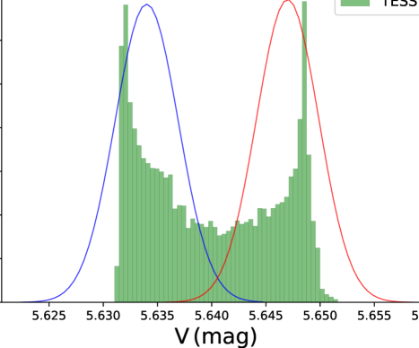
Figure 1: Magnitude histogram for HD 72968 using 50 bins for 10,703 TESS data points, showing a bimodal relationship possibly caused by a pulsation affecting its brightness.

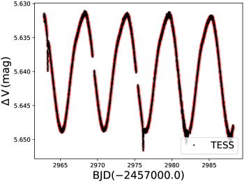
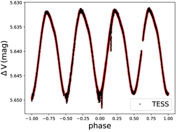
Figure 2: (Left) TESS photometric flux transformed to magnitude according to Eq. 2, distributed over BJD(-2457000.0). (Right) Light curve for HD 72968, according to Eq. 3.

Subsequently, we conducted a photometric analysis of the TESS light curve, considering all 10703 quality TESS data points. The dataset was analyzed using the Phase Dispersion Minimization (PDM-IRAF) algorithm of (Stellingwerf, 1978). The minimum and maximum values were determined through light curve analysis to establish the correct period. In this study, we examined data covering periods ranging from 1 to 20 days. Once the period was identified within the range of 10.9 to 11.7 days, decimal adjustments were made in increments of $\pm 0.1$ days until achieving optimal precision in the period value. Consequently, analyzing the light curve of HD 72968, we obtained an orbital period of $\mathrm{P=11.307\pm 0.005,\mathrm{d}}$, thus corroborating the previously reported value of 11.305 days for the orbital period of the same chemically peculiar star, according to the photometric light curve studies by Maitzen, Albrecht, & Heck (1978) and Adelman (1998). Therefore, we determined the following ephemeris for the light curve, which will be used for further analysis in the document:

$$\mathrm{HJD_{min}=2459976.4413447+11.307(5)\cdot E},$$ (3)

where $\mathrm{HJD_{min}}$ corresponds to the Heliocentric Julian Date, the time HJD = 2459976.4413447 corresponds to the reference epoch, P is the orbital period of the star HD 72968, and E is the number of complete epochs elapsed since 2459976.4413447, which is the reference epoch.

For the graphical representation shown in Figure 2, the advanced software PHOEBE was used. This software utilizes previously obtained parameters, such as the period $\mathrm{P}=11.307\pm 0.005,\mathrm{d}$ and the time in BJD 2976.14736220 of the minimum apparent magnitude. This allows for the generation of the magnitude-phase plot, centered at 0, with positive and negative extremes of 1 and -1, respectively.

0.3 Wavelet Analysis of Data

For a more localized and adaptive representation of the characteristics of the photometric data, we decided to use the mathematical technique that employs wavelet functions to analyze and process signals and data. In brief, unlike other frequency analysis techniques, such as the Fourier transform, which uses sinusoidal functions, wavelet data analysis provides a more localized and adaptive representation of a signal’s characteristics. Wavelet functions are small waves (wavelets) that are localized in both time and frequency.

They are generated from scaling functions that satisfy the recursion relation Auger & Tangborn (2004), presented in equation 7. In brief, this transform operates by using functions called wavelets, which are small waves that shift and scale to adapt to different parts of the signal, in this case, to frequencies corresponding to the star’s period.

$$\mathrm{\phi(x)=\sum\limits_{k}c_{k}\phi(2x-k)},$$ (4)

where $c_{k}$ is a finite set of filter coefficients. For the analysis of 10,703 TESS data points, the normalized wavelet power spectrum was used, employing the Morlet wavelet ($\omega=6$), which is a complex exponential (Fourier) wave given by equation 5.

$$\mathrm{\psi(t)=\exp\left(i\omega_{0}t\right)\exp\left(-\frac{t^{2}}{2\sigma^{2}}\right)},$$ (5)

where $\mathrm{\omega_{0}}$ is the frequency and $\sigma$ is a support measure for the wavelet. For the Morlet mother wavelet, the base scale parameters were adjusted to $s_{0}=60*dt$, the scale factor $dj=1/12$, the total number of scales $J=7/dj$, and $\alpha=0.77$. The normalized Morlet wavelet power spectrum is presented in Figure 3.

Thus, for a total of 10703 photometric data points provided by TESS, with a cadence of 3.33 minutes and a $\mathrm{T_{0}=2962.8045771}$, we performed wavelet data analysis by applying the wavelet transform. This involves shifting and scaling the mother wavelet function to adapt to different parts of the signal, as mentioned earlier. This shifting or translation moves the wavelet function along the time axis, allowing different parts of the signal to be analyzed at different moments. Meanwhile, the scaling allows the wavelet function’s scale to be adjusted to analyze the signal at different frequencies. Due to the pulsating nature of this star, as it belongs to the CP family, it was necessary to consider a function with a higher frequency capable of capturing fine details in the signal. It is worth noting that this could have caused the loss of information about low-frequency components. Our mother wavelet function is of order 6, and we have considered 12 sub-octaves per octave. This means that one frequency interval is double the frequency of another interval. Therefore, when referring to ”octaves” in the context of wavelets, we are discussing scales that vary in frequency logarithmically. Each octave represents a frequency range that is double that of the previous octave. The term ”sub-octave” refers to frequency intervals that are smaller than an octave. Instead of doubling the frequency, a sub-octave could represent a fraction of the frequency of the previous octave. This allows for a more detailed analysis of low frequencies without covering as broad a range as a full octave.

Once a 30th-degree polynomial was fitted within the wavelet function, we noticed the existence of a new period within the light curve that had not been previously detected using the PDM-IRAF task. This period is $\mathrm{P_{2}=2.7,\mathrm{d}}$ and is possibly related to internal pulsations of the star (see Fig. 3-B,C). Additionally, we observed two anomalies or changes in the morphology of the light curve at $\mathrm{BJD=2976.15}$ and $\mathrm{BJD=2963.31}$, where the star’s brightness drops over a short period. We speculate that during pulsation, the star ejects a small amount of material, causing a brief eclipse at those reported moments. Furthermore, starting from $\mathrm{BJD=2980}$, we noticed that during the star’s minima, a variation in the morphology appeared, which is more extended and seems to be remnants of the second mini-eclipse or anomaly corresponding to $\mathrm{BJD=2963.31}$ (see Fig. 3-A).

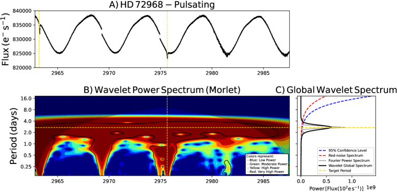
Figure 3: Plot A: Temporal evolution of the observed flux (flux vs. time), with the detected variabilities marked by dashed yellow lines. Plot B: Normalized wavelet spectrum. The gray area represents the cone of influence. The horizontal dashed yellow line corresponds to the detected period $P_{2}$ of the star, $P_{2}=2.7$ days. The vertical dashed yellow line near $\mathrm{BJD=2976.15}$ highlights an anomaly in HD 72968 as it enters its minimum magnitude. The black contour lines enclosing various regions of the plot indicate a 95% statistical significance level. A jet color palette is used, where blue represents low wavelet power, red indicates high wavelet power, and intermediate power values are shown in green and yellow, respectively. Plot C: Global wavelet power spectrum. The dashed black line shows the average power spectrum, with a prominent peak at $P_{2}=2.7$ days. The solid gray line represents the Fourier Transform, included for comparison with the wavelet analysis. Dashed red lines indicate the noise level, with the average power peak lying above it, suggesting the presence of a real signal. The dashed blue lines represent the 95% significance threshold; similarly, the average power peak lies above this threshold, providing additional evidence for a real oscillation. Dashed yellow lines mark the period of interest.

0.3.1 Colorimetry Method

We conducted a search for photometric data provided by ExoFOP-TESS (Akeson & Christiansen, 2019) for other bands and summarized some of these in Table 1. In the color-color graphical representation shown in Figure 4, we have plotted 27 spectral type variants spanning a temperature range from 35900 K to 4560 K (Cox, 2000). The color difference was $\mathrm{J-H}=-0.046\pm 0.069$ (mag) and $\mathrm{H-K}=0.064\pm 0.058$ (mag), giving us clues that the star fluctuates within a fairly wide temperature range (see Table 2). Placing it for the $\mathrm{J-H}$ difference at $\mathrm{13550\pm 550,\rm{K}}$, while for the $\mathrm{H-K}$ difference, it is $\mathrm{5430\pm 380,\rm{K}}$.

From the photometry conducted for the star HD 72968, an initial estimate of its effective temperature was obtained, which was 10,700 K according to UBV data (Hensberge & De Loore, 1974). By plotting the color-color graph shown in Figure 4 with the photometric data $\mathrm{J-H,and,H-K}$ according to their position relative to main sequence stars, an estimated effective temperature of $\mathrm{13550\pm 550,\mathrm{K}}$ was obtained. It is important to note that the difference between main sequence stars and chemically peculiar stars is that in chemically enriched stars, according to Adelman & Kaewkornmaung (2005), anomalous photospheric abundances are produced by hydrodynamic processes, particularly radiative diffusion and gravitational settling in radiative envelopes containing strong magnetic fields.

This significant discrepancy between the initial estimate based on UBV data and the result obtained using data from Cox (2000) is due to various factors that affect information acquisition, such as different types of filters and bands, instrumental calibrations, instrument sensitivity due to constant technological updates, atmospheric correction, and reddening correction. This highlights the importance of considering different data sources and methods when analyzing the effective temperature of the star.

Table 1: Photometric summary for the mCP star HD 72968 in different bandwidths.

Band	Value (mag)	error (mag)	$\lambda_{\textrm{eff}}$ (Å)
TESS	5.744	0.007	7452.64
ExoFOP-B	5.697	0.022	4400
ExoFOP-V	5.733	0.023	5500
Gaia	5.714	0.001	5857.56
2MASS-J	5.708	0.029	12350
2MASS-H	5.754	0.040	16620
2MASS-K	5.690	0.018	21590
WISE1	5.720	0.146	33526
WISE2	5.634	0.053	46028
WISE3	5.808	0.016	115608
WISE4	5.760	0.047	220883.83

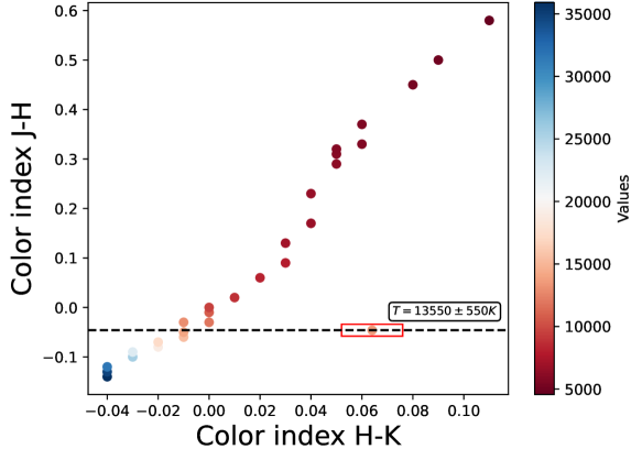
Figure 4: Color-temperature comparison of HD 72968 with respect to 27 spectral types of main sequence stars.

Table 2: Intrinsic Colors and Effective Temperatures for the Main Sequence (Class V)^a.

Spectral type	V-K	J-H	H-K	K-L	K-L’	K-M	$T_{efl}$
O9	-0.87	-0.14	-0.04	-0.06			35900
09.5	-0.85	-0.13	-0.04	-0.06			34600
BO	-0.83	-0.12	-0.04	-0.06			31500
B1	-0.74	-0.10	-0.03	-0.05			25600
B2	-0.66	-0.09	-0.03	-0.05			22300
B3	-0.56	-0.08	-0.02	-0.05			19000
B4	-0.49	-0.07	-0.02	-0.05			17200
B5	-0.42	-0.06	-0.01	-0.04			15400
B6	-0.36	-0.05	-0.01	-0.04			14100
B7	-0.29	-0.03	-0.01	-0.04			13000
B8	-0.24	-0.03	0.00	-0.04			11800
B9	-0.13	-0.01	0.00	-0.03			10700
AO	0.00	0.00	0.00	0.00	0.00	0.00	9480
A2	0.14	0.02	0.01	0.01	0.01	0.01	8810
AS	0.38	0.06	0.02	0.02	0.02	0.03	8160
A7	0.50	0.09	0.03	0.03	0.03	0.03	7930
FO	0.70	0.13	0.03	0.03	0.03	0.03	7020
F2	0.82	0.17	0.04	0.03	0.03	0.03	6750
F5	1.10	0.23	0.04	0.04	0.04	0.02	6530
F7	1.32	0.29	0.05	0.04	0.04	0.02	6240
GO	1.41	0.31	0.05	0.05	0.05	0.01	5930
02	1.46	0.32	0.05	0.05	0.05	0.01	5830
04	1.53	0.33	0.06	0.05	0.05	0.01	5740
06	1.64	0.37	0.06	0.05	0.05	0.00	5620
KO	1.96	0.45	0.08	0.06	0.06	-0.01	5240
K2	2.22	0.50	0.09	0.07	0.07	-0.02	5010
K4	2.63	0.58	0.11	0.09	0.10	-0.04	4560

NOTE: ^aColors provided in the Johnson-Glass system, as established by (Bessell & Brett, 1988). The references used are: O, B, [2]; A, F, O, K, [1]; K, M, [3]. K-M from [2] was not used due to a large discrepancy compared to (Bessell & Brett, 1988). Approximate uncertainties (one standard deviation): $\pm$0.02 (O-K); $\pm$0.03 (M). ${}^{b}T_{{eff}}$ is an average of values from the following sources: for O, B, [4]; for B, A, F, O, K, [5]; for B, O, K, [6]; for A, F, [7]; for A, F, O, K, [8]; for A, F, O, [9]; for O, K, [10]; for K, M, [3]; for M, [11], [7], [12]. Approximate uncertainties (one standard deviation): $\pm$1000 K (O9-B2); $\pm$250 K (B3-B9); $\pm$100 K (A0-M6).

0.4 Spectroscopy

The corrected and wavelength-calibrated spectrum was obtained from the European Southern Observatory (ESO) database for the star HD 72968. The processing of the obtained spectra was carried out using IRAF; the spectra were trimmed and continuum-normalized using the “chebyshev“ fitting function (Chebyshev polynomial) and were not flux-calibrated. Rosales et al. (2023) states, “Flux calibration of the spectra is not necessary as it does not affect line strength measurements and radial velocities”. For the chemical composition analysis of the chemically peculiar star HD 72968, the spectrum presented in Table 3 was used.

Table 3: Summary of the observed spectrum. N is the number of extracted spectra, HJD is the reference system used to specify the observation time, and $\phi_{0}$ refers to the orbital period determined using equation 3. S/N stands for signal-to-noise ratio.

Date	Instrument	N	Exposure time (s)	HJD	$\mathrm{\phi_{0}}$	S/N
20-12-2005	UVES	1	37.5014	2403724.74899141	0.948468	150.7

After normalization, the Doppler effect correction was applied by modifying the radial velocity ($\mathrm{km\,s^{-1}}$) of the extracted spectra in IRAF.

In addition to the Doppler effect correction, chemical element identification was performed in IRAF for absorption lines by specifying the wavelength in angstroms. Using the VizieR astronomical catalog, the main chemical elements associated with the A2p spectral type of HD 72968 were identified for use in the present investigation.

Table 4: Chemical elements identified in the star HD 72968 according to information obtained from VizieR, where the determined chemical element, wavelength in angstroms, spectral type range, and equivalent width (EW) of the absorption lines with the associated error ($\pm$ Rms) are represented.

Chemical element	Wavelength (Å)	Spectral type	EW $\pm$ Rms
Sr II	4077.7140	A0V-M2Ia	0.914 $\pm$ 0.098
H $\delta$	4101.7370	O9V-M2Ia	2.506 $\pm$ 0.019
Cr II	4824.1300	A0-A3V;A0-G0IV;A0-G0Ia	$0.259\pm 0.033$
H $\beta$	4861.3320	O9V-M2Ia	$11.720\pm 0.060$

In Figure 5, two significant absorption lines corresponding to Sr II and H $\delta$ are observed, as established by Babcock (1958) for HD 72968 of spectral type A2p, where the predominant chemical element is Sr (Strontium). Morgan (1931) defined that, in general, stars exhibit approximately equal chemical abundances. However, some stars do not fit within the bidimensional temperature and pressure scale, such as those displaying strong Sr (Strontium) lines at 4077 Å. According to the Henry Draper catalog, these are classified as chemically peculiar stars. Additionally, the Balmer line H $\delta$ at 4101 Å is present, which is characteristic of spectral type A stars, such as HD 72968.

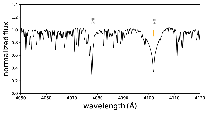
Figure 5: Spectrum of the star HD 72968 in the range of 4050 Å to 4120 Å, showing chemical elements such as Strontium Sr II at 4077.7 Å and H $\delta$ at 4101.7 Å.

In Figure 6, the spectrum of HD 72968 is presented in the range of 4800 Å to 4900 Å, where two prominent absorption lines are identified as Cr II at 4824.1 Å and H $\beta$ at 4861.3 Å. The Sr II and Cr II elements present in HD 72968 correspond to the Sr-Cr spectral type classification for this star, as determined by Hensberge & De Loore (1974).

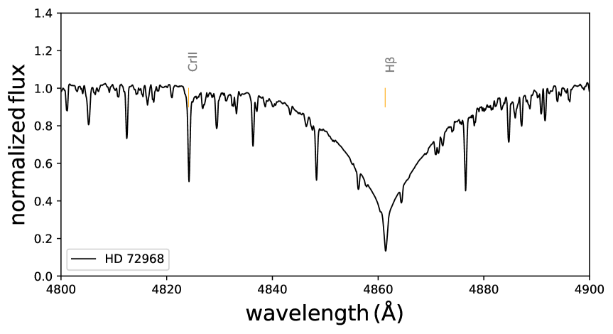
Figure 6: Spectrum of the star HD 72968 in the range of 4800 Å to 4900 Å, showing chemical elements such as Chromium II at 4824.1 Å and H $\beta$ at 4861.3 Å.

Chemical abundance

We have performed the chemical abundance analysis presented in Table 5 for the star HD 72968 in the wavelength range from 4800 Å to 5000 Å using the IRAF software. The wavelengths of each absorption line, equivalent widths, and errors were obtained. Then, through the astronomical catalog VizieR, the chemical elements present were identified based on the peculiar chemical characteristics of HD 72968.

Using the previously compiled data from the NIST Atomic Spectra Database Lines Data, we obtained the parameters $E_{\mathrm{low}}$ (cm^-1), $E_{\mathrm{high}}$ (cm^-1), $g_{k}A_{ki}$ ($10^{8}$ s^-1), $f_{ik}$, and $\log(g_{i}f_{ik})$, which are essential for the chemical abundance analysis of the chemically peculiar star.

To derive the abundance values from the parameters retrieved from NIST, the software ABUNDANCE SPECTRUM was used. The stellar parameters of HD 72968, including its rotational velocity, were input to ensure a more accurate determination of the star’s chemical abundances.

The chemical abundance values [X/H] of each element relative to the solar abundance are presented in Table 6.

Table 5: Equivalent width of the most representative spectral lines of HD 72968.

Elements	Wavelength (Å)	Z	Equi. Width (Å)	error (Å)
Ti II	4805.1050	22	0.1192	0.01271
Ti I	4812.2400	22	0.1206	0.01182
Cr II	4824.1300	24	0.2590	0.01900
Ni I	4829.6800	28	0.1011	0.01289
Cr II	4836.1250	24	0.1261	0.03728
Cr II	4848.4100	24	0.1481	0.00625
H$\beta$	4861.3320	1	11.720	0.06000
Cr II	4876.4100	24	0.2038	0.00629
Cr II	4884.5700	24	0.1014	0.01266
Fe I	4891.5500	26	0.0718	0.01080
S II	4901.6500	27	0.1049	0.02310
Ni I	4912.4900	28	0.0812	0.01145
Nd II	4920.2800	60	0.1717	0.03485
Fe II	4923.9210	26	0.1776	0.04333
Fe I	4930.3310	26	0.0444	0.01231
Cr I	4936.1550	24	0.0539	0.01418
Ti I	4941.0150	22	0.0512	0.01143
Ba II	4957.1500	56	0.1981	0.01404
Sr I	4971.6680	38	0.0481	0.00947
Ti I	4977.7310	22	0.1447	0.02377
Y II	4982.1300	39	0.0374	0.00881

Table 6: Atomic parameters and chemical abundances for HD 72968

Elements	$\lambda$ (Å)	Z	$E_{\mathrm{low}}$ (cm-1)	$E_{\mathrm{high}}$ (cm-1)	$g_{k}A_{ki}$ ($10^{8}$ s-1)	$f_{ik}$	$\log(g_{i}f_{ik})$	[X/H]	$\sigma$
Ti II	4805.0928	22	16625.2441	37430.681	2.200e7	1.900E-2	-1.120	-0.387	0.179
Ti I	4812.8934	22	6842.9620	27614.679	9.900e4	3.100E-5	-3.460	2.678	0.179
Cr II	4824.1308	24	31219.3322	51942.664	1.700e7	5.900E-3	-1.230	0.703	0.179
Ni I	4829.0230	28	28569.2030	49271.540	1.300e8	9.300E-2	-0.330	-0.557	0.220
Cr II	4836.2295	24	31117.3254	51788.815	1.600e6	9.400E-4	-2.250	0.990	0.182
Cr II	4848.2497	24	31168.5755	51788.815	2.100e7	9.200E-3	-1.130	-0.001	0.179
H$\beta$	4861.3330	1	82259.1580	102823.904	2.694e8	1.194E-1	-0.020	4.092	0.188
Cr II	4876.4892	24	31168.5755	51669.406	9.600e6	4.300E-3	-1.470	0.636	0.179
Cr II	4884.6035	24	31117.3254	51584.100	2.300e6	1.400E-3	-2.080	0.668	0.179
Fe I	4891.4920	26	22996.6740	43434.627	2.160e8	8.590E-2	-0.112	-2.597	0.179
S II	4901.2780	27	130134.1580	150531.304	9.600e7	9.600E7	-0.460	10.831	0.180
Ni I	4912.0180	28	30392.0030	50744.552	4.500e7	5.400E-2	-0.790	-0.014	0.179
Nd II	4920.6850	60	513.3300	20830.030	7.100e7	2.580E-2	-0.588	1.270	0.182
Fe II	4923.9212	26	23317.6351	43620.984	1.700e7	1.040E-2	-1.210	-1.745	0.184
Fe I	4930.3149	26	31937.3250	52214.345	1.720e7	2.100E-2	-1.201	-0.690	0.179
Cr I	4936.3357	24	25106.2953	45358.584	1.300e8	6.600E-2	-0.340	-0.125	0.179
Ti I	4941.5707	22	17423.8560	37654.690	2.600e7	1.900E-2	-1.010	1.030	0.179
Ba II	4957.0950	56	48258.6170	68426.095	4.100e8	2.500E-1	0.190	4.162	0.179
Sr I	4971.6680	38	14898.5450	35006.908	3.900e6	2.900E-3	-1.800	3.239	0.179
Ti I	4977.7275	22	16267.4800	36351.365	4.850e7	1.640E-2	-0.740	1.216	0.180
Y II	4982.1300	39	8328.0390	28394.177	1.380e7	7.300E-3	-1.290	0.408	0.179

The uncertainty in the chemical abundances, $\sigma$, was determined based on the error propagation of several parameters obtained in this work, including the uncertainty in the effective temperature ($E_{T_{\mathrm{eff}}}$), surface gravity ($E_{logg}$), rotational velocity ($E_{v\sin i}$), and the equivalent width uncertainty derived from Gaussian fitting in IRAF ($E_{\mathrm{eqw}}$), using equation 6.

$$\mathrm{\sigma=\sqrt{(\frac{E_{T_{eff}}}{T_{eff}})^{2}+(\frac{E_{logg}}{logg})^{2}+(\frac{E_{v\sin i}}{v\sin i})^{2}+({E_{\mathrm{eqw}}})^{2}}},$$ (6)

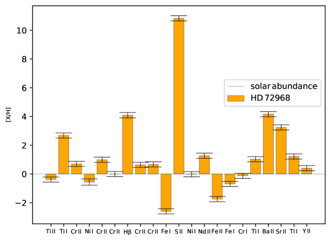
Figure 7: Comparison of the chemical abundances of the star HD 72968 with those of the Sun. Positive values indicate an overabundance of certain elements in the star, while negative values reflect a deficiency. Notable differences in elements such as barium (Ba), sulfur (S), and strontium (Sr) are characteristic of chemically peculiar stars.

Numerical method

Obtained the spectrum corrected for the Doppler effect, the search for the star’s data in the Gaia DR3 Mission database was carried out to obtain the metallicity [M/H] in order to download the stellar atmospheres from ATLAS9. The acquisition of the ATLAS9 models was performed using the code ”am10ak2c125odfnew” (Castelli & Kurucz, 2003).

In the present method, the chi-square statistical model was used to obtain the best fit between the observed spectrum and the theoretical spectrum obtained from the SPECTRUM software with stellar atmosphere models from ATLAS9.

By estimating different stellar models according to temperatures in the SPECTRUM software, it was determined that the best chi-square value was estimated between the effective temperatures of $\mathrm{T_{eff}}$ = 7000 K to 15000 K.

For the elaboration of the table, the wavelength range from 4800 Å to 4900 Å was used, defining the effective temperatures of $\mathrm{T_{eff}}$ = 7000 K to 15000 K in steps of 250 K. For the surface gravity values, they were established from logg = 0.0 dex to 5.0 dex in steps of 0.5 dex, the microturbulence velocity set at 0.0 $\mathrm{km\,s^{-1}}$ according to ATLAS9 stellar models, solar metallicity value defined as [M/H] = 0.00, and spectral resolution of r = 0.01483899664.

The mixing length parameter, which corresponds to the disruption and dispersion of bubbles traveling in a convective fluid over a distance “l”from their equilibrium position in a scale atmosphere “H”(Rosales et al., 2023), was set at 1.25 l/H according to the ATLAS9 stellar models. The rotational velocity value was established based on the references of Preston (1971), defined as 16 $\mathrm{km\,s^{-1}}$, determined through the extended helium abundance in the stellar atmosphere $\mathrm{H_{e}}$(ext) = 0.7 kilogauss.

The rotational velocity value according to Hensberge & De Loore (1974) was in the range of 10 to 12 $\mathrm{km\,s^{-1}}$, following the criterion of weak magnetic lines of specific chemical elements such as Fe I and Cr I, as well as the common rotational broadening in all lines of HD 72968. Knowing the rotational velocity data, a range from 0 to 100 $\mathrm{km\,s^{-1}}$ in steps of 1 $\mathrm{km\,s^{-1}}$ was established to determine which value best fit the chi-square in the theoretical spectrum. Evaluating the aforementioned parameters, the best model converged to the following value $\mathrm{v_{sini}=8\mathrm{km\,s^{-1}}}$, which showed the best fit determined through the chi-square statistical method.

The ATLAS9 grid, consisting of effective temperature versus surface gravity, was constructed, obtaining the best chi-square with the parameters shown in Table 7.

Table 7: Parameters established through the mathematical method for the best chi-square fit in the theoretical spectrum for HD 72968, which include: effective temperature, surface gravity, microturbulence velocity, rotational velocity, mixing length, metallicity, best chi-square fit, and spectral resolution.

Parameters	Values
$\rm{T_{eff}}$	$\rm{10250\pm 250\,K}$
$\rm{log{g}}$	$\rm{4.0\pm 0.5\,dex}$
$\rm{*V_{micro}}$	$\rm{0.0\,{km\,s^{-1}}}$
$\rm{v\sin{i}}$	$\rm{8\pm 1\,{km\,s^{-1}}}$
$\rm{[l/H]}$	$\rm{1.25}$
$\rm{[M/H]}$	$\rm{0.00}$
$\rm{\chi^{2}}$	$\rm{18.5}$
$\rm{r}$	$\rm{0.01483899664}$

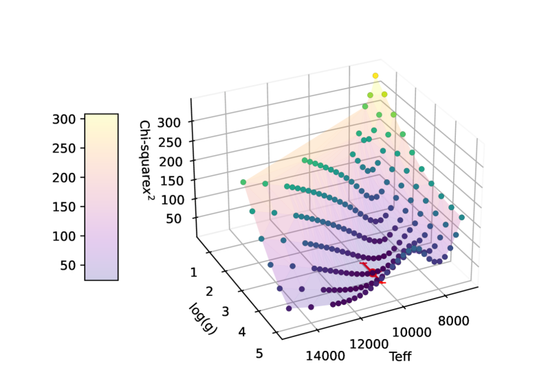
Figure 8: Chi-square analysis to determine the best normalized spectrum in reference to the observed spectrum of HD 72968. The $\mathrm{\chi^{2}}$ graph was created using only 3 degrees of freedom, showing the minimum chi-square value of $\mathrm{\chi^{2}}$ = 18.5, represented by a red point. Each point within the graph represents an effective temperature associated with its surface gravity.

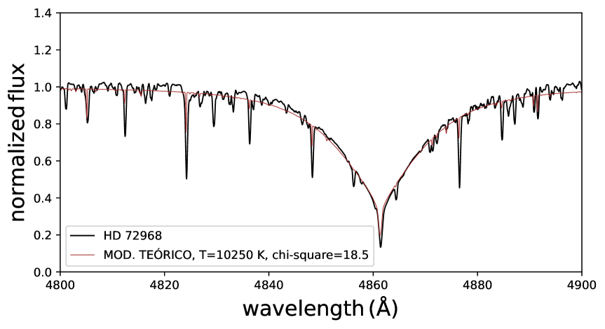
Figure 9: Comparison between the observed spectrum (Black) of CP HD 72968 and the theoretical spectrum (Red) with the smallest standard deviation, from 4800.0 Å to 4900.0 Å. The obtained temperature is $\mathrm{T_{eff}=10250\,K}$, and $\mathrm{\log g=4.0\,dex}$.

In Figure 9, it can be seen that the theoretical spectrum from the SPECTRUM software, starting at 4800.0 Å, ending at 4900 Å, and having a resolution of r = 0.01483899664, exhibits spectral similarities in the Balmer line and in the absorption lines of the observed spectrum. It is important to highlight that modeling stellar atmospheres with ATLAS9 and using SPECTRUM to generate the graph serve as guidance and provide direction for the research, but are not meant to be taken as absolute results. ”Models like ATLAS9 and MARCS serve as starting points for our technique, which is by no means limited to them” (Westendorp Plaza, Asensio Ramos, & Allende Prieto, 2023).

Comparative method

To determine thermal criteria, stars of the same luminosity class corresponding to different spectral types are compared whenever possible. However, since the temperature sequence covers such a wide range from O to M,it is logical to understand that these criteria gradually vary within a certain range where they respond perfectly to some criterion. It often happens that upon reaching a certain spectral type, the difference between the intensities of the compared lines reaches a proportion so large that it can no longer be applied as an indicator (Jaschek & Jaschek, 1968).

The theoretical effective temperature $\mathrm{T_{eff}=10250\pm 250\,K}$ was obtained through spectral analysis using the Spectrum software. A comparative method with other peculiar stars was then applied to define the upper and lower limits for the star HD 72968. For this comparison method, data from two chemically peculiar stars with similar characteristics to the studied star HD 72968 were extracted from the SIMBAD database using a special search type from the Hipparcos catalog, which has been identifying bright stars with precise and independent information for the past thirty years (Brandt, 2021). The selected peculiar A-type stars were HD 220825 and HD 223640.

HD 220825 is cataloged as a chemically peculiar star of spectral type Ap, with an effective temperature of 9470 K, a surface gravity of logg = 4.20 dex, and a stellar radius of 1.71 $\mathrm{R_{\odot}}$, determined through spectroscopic methods according to Romanovskaya et al. (2021). HD 223640 is a chemically peculiar star of spectral type Ap, with an effective temperature of 12340 K, determined photometrically by Lanz (1985) using the Blackwell-Shallis method, one of the most precise methods for determining a star’s effective temperature through photometry, developed by Blackwell & Shallis (1977). Additionally, the temperature value of 12340 K was confirmed through the empirical method for determining effective temperatures and angular diameters in milliarcseconds, established by Megessier (1988).

To compare the spectral characteristics, two spectra were used, as presented in Table 8. The spectra used in this research fall within the blue arm, corresponding to wavelengths from 300 nm to 500 nm, according to the European Southern Observatory (ESO) database, where ultraviolet light is used for various astrophysical studies. These spectra are cataloged in scientific spectra, and diffraction gratings of 437 l/mm (lines per millimeter) were used for all spectra.

Table 8: Summary of UVES spectra extracted for comparison with the star HD 72968. N represents the number of extracted spectra, HJD is the Heliocentric Julian Date, S/N corresponds to the signal-to-noise ratio, and R is the instrument resolution.

Object	Date	HJD	N	Exposure Time (s)	S/N	R
HD 220825	17-05-2016	2457525.91	1	28.0017	149.7	80 000
HD 223640	14-08-2002	2452500.94	1	40.0009	151.33	80 000

The spectra of the stars HD 220825 and HD 223640 were acquired from the European Southern Observatory (ESO) database, normalized, and wavelength-calibrated for subsequent comparison with the star HD 72968 to estimate the effective temperature. Figure 10 shows the comparison between two chemically peculiar stars with similar spectral types. The spectrum of the star HD 220825 is shown in orange, while the spectrum of the star HD 72968 is shown in black. The chi-square value obtained between both stars was $\mathrm{\chi^{2}=34.3}$, which is greater than the theoretical chi-square value, leading us to consider the star HD 220825 as the reference for the lower effective temperature due to its spectral visual similarity.

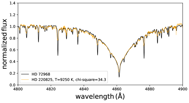
Figure 10: Comparison of the chemically peculiar star HD 220825 (orange) with 9250 K against the spectrum of the chemically peculiar star HD 72968 (black).

Figure 11 shows the comparison between two chemically peculiar stars with similar spectral types. The spectrum of the star HD 223640 is shown in blue, while the spectrum of the star HD 72968 is shown in black. The chi-square value obtained between both stars was $\mathrm{\chi^{2}}=66.1$, which is greater than the theoretical chi-square value, leading us to consider the star HD 223640 as the reference for the upper effective temperature. Since the effective temperature is higher than the theoretical effective temperature of 10250 K, the chi-square value is also higher. The blue spectrum near the wavelength 4861.3 Å presents spectral disparity compared to the black spectrum.

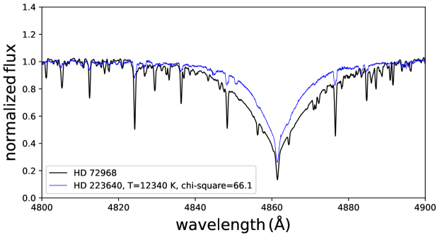
Figure 11: Comparison of the chemically peculiar star HD 223640 (blue) with a correction factor relative to the chemically peculiar star HD 72968 (black).

Figure 12 shows the complete comparison of the spectra used for the spectral comparison with the chi-square statistical technique. The black spectrum corresponds to the observed spectrum of HD 72968, the red spectrum belongs to the theoretical spectrum for the star HD 72968, the orange spectrum corresponds to the peculiar star HD 220825, and the blue spectrum belongs to the star HD 223640.

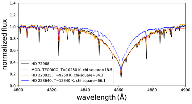
Figure 12: Spectral comparison of the star HD 72968 (black) with respect to the theoretical spectrum (red), the star HD 220825 (orange), and the star HD 223640 (blue).

0.5 Spectral distribution of energy SED

The spectral energy distribution (SED) is a graphical representation or a curve that relates the flux emitted by a star in units of Flux $\mathrm{(ergs^{-1}cm^{-2}\AA {}^{-1})}$ and the wavelength in units of Angstrom (Å). Within the SED, two variables are presented: the photometric points emitted by the star, in this case, HD 72968, and a continuous spectrum ranging from the ultraviolet to the far-infrared, which corresponds to the stellar model of the best chi-square fit between the variables.

In Table 9, the data of fluxes and photometric flux errors, wavelengths, and the information of the filters used for the observation of the star HD 72968 are indicated, extracted from SED VizieR.

To define the SED, the Kurucz ODFNEW / NOVER (2003) model Castelli & Kurucz (2003) was selected, as this model encompasses stars of different spectral types, including stars with chemical abundances. Additionally, it presents improved opacities and abundances in the energy spectra. The values obtained through the spectroscopic study were then input: effective temperature $\mathrm{10000\,a\,10500\,K}$, surface gravity logg $\mathrm{3.5\,\,a\,\,4.5\,dex}$, solar metallicity of 0.0, and relative abundance of alpha elements of 0.0, simulating the solar chemical abundance. Furthermore, we considered the reddening caused by extinction in the line of sight due to interstellar dust, such as $\mathrm{E(B-V)_{SFD}}$ and $\rm{Av_{SFD}}$, which were calculated using equation 7 through IRSA.

$$\mathrm{Av_{SFD}/E(B-V)_{SFD}=0.31},$$ (7)

the best fit within the range of free parameters that we set based on previous results leads to a convergence of effective temperature $\mathrm{T_{eff}=10000\,K}$, a surface gravity of logg = 4.5 dex, metallicity = 0.5, and a visual extinction of Av = 0.195.

It is important to highlight the variation in metallicity from 0.0 to the resulting metallicity of 0.5, which is higher than solar. This suggests that the star HD 72968 exhibits chemical abundance anomalies or another effect, such as rapid rotation, which could increase the metallicity value of HD 72968 relative to solar metallicity Viswanath et al. (2023).

Obtaining the photometric parameters through the first construction of the SED, we have used equation 8 obtained from Kunzli et al. (1997), which relates the initial metallicity $\mathrm{[M/H]_{0}}$ and the effective temperature $\mathrm{T_{eff}}$ to estimate the final metallicity [M/H] of HD 72968.

$$\mathrm{[M/H]=0.260+1.193\cdot[M/H]_{0}\mathrm{-}3.4e-5\cdot\mathrm{T_{eff}}},$$ (8)

where $\rm{M/H}$ is the actual stellar metallicity of the chemically peculiar star estimated to be $\rm{M/H=0.517\pm 0.008}$, which was adjusted to the approximate value of the effective temperature determined through spectroscopy, $\mathrm{{M/H_{0}}}$ is the estimated initial stellar metallicity $\mathrm{M/H_{0}=0.5}$ according to the SED, and $\mathrm{T_{eff}}$ is the effective temperature of the star estimated to be $\mathrm{T_{eff}=\rm{10000\pm 250\,K}}$. With the values obtained from the SED, it was verified that the star HD 72968 exhibits chemical abundances with a value of $\mathrm{M/H>0}$, which is the solar metallicity reference for all stars.

Table 9: Photometric summary for the mCP star HD 72968 in different bandwidths obtained from the SED of VizieR.

wavelength	Flux	Flux error	Filter
$(\mu m)$	$(ergs^{-1}cm^{-2}\mu m^{-1})$	$(ergs^{-1}cm^{-2}\mu m^{-1})$
0.4203	3.46e-7	7.13e-13	HIP:BT
0.4442	3.40e-7	1.35e-12	Johnson:B
0.5036	2.21e-7	5.95e-13	GAIA3:Gbp
0.5319	2.06e-7	5.64e-13	HIP:VT
0.5319	2.08e-7	1.13e-12	HIP:VT
0.613	7.19e-8	4.89e-14	PAN-STARRS/PS1:r
0.762	6.97e-8	3.93e-13	GAIA3:Grp
0.7485	4.40e-8	4.01e-14	PAN-STARRS/PS1:i
0.7635	4.23e-8	3.93e-14	SDSS:i
1.239	1.61e-8	5.08e-13	2MASS:J
1.25	1.61e-8	3.60e-13	Johnson:J
1.63	5.86e-9	3.49e-13	Johnson:H
1.65	5.77e-9	3.45e-13	2MASS:H
2.164	2.29e-9	8.31e-14	2MASS:Ks
2.19	2.16e-9	8.21e-14	Johnson:K
3.35	4.59e-10	4.47e-14	WISE:W1
3.35	4.30e-10	8.05e-14	WISE:W1
3.4	3.84e-10	1.76e-13	Johnson:L
4.6	1.38e-10	1.63e-14	WISE:W2
4.6	1.16e-10	7.15e-15	WISE:W2
5.03	1.04e-10	2.56e-14	Johnson:M
8.61	1.26e-11	3.48e-15	AKARI:S9W
11.56	3.10e-12	5.19e-16	WISE:W3
22.09	2.48e-13	2.04e-16	WISE:W4

Finally, for better accuracy, we developed a theoretical spectral energy distribution (SED) to obtain the best fit. The statistical technique of chi-square was applied, using the total theoretical spectral flux from Fitzpatrick & Massa (2005) with equation 9, complemented by equations 10 and 11 obtained from Rosales Guzmán et al. (2018) for the determination of the partial stellar flux and the normalized extinction curve, respectively, over a wavelength range from 1005 Å to 1600000 Å covering from ultraviolet to infrared.

For the total theoretical spectral flux, the photometric data offered by the VizieR SED and theoretical photometric models gathered from VOSA were compared, with effective temperature parameters ranging from 10000 K to 10500 K in steps of 250 K, surface gravity from 3.5 to 4.5 dex in steps of 0.5 dex, and solar

$$\mathrm{f\lambda=f_{\lambda,0}10^{-0.4E(B-V)[k(\lambda-V)+R(V)]}},$$ (9)

where,

$$\mathrm{f_{\lambda,0}=\left(\frac{R_{1}}{d}\right)^{2}\cdot f_{\lambda,1}},$$ (10)

$\mathrm{E(B-V)=0.0380\pm 0.0006}$ corresponds to the data obtained from IRSA, where $\mathrm{R(V)=A_{v}/E(B-V)}$. The value of $\mathrm{k(\lambda-V)=E(\lambda-V)/E(B-V)}$ was determined using equation 11.

where $\mathrm{R_{1}}$ is the radius to be determined, adjusted from $\mathrm{2.00\,to\,2.10\,R_{\odot}}$, corresponding to the radius of the star HD 72968, $\mathrm{d=107.531\pm 1.135\,pc}$ is the photometric distance obtained from the Gaia DR3 mission, and $\mathrm{f_{\lambda,1}}$ is the theoretical flux of the star related to the wavelength.

$$\mathrm{k=}\left\{\begin{array}[]{ll}\mathrm{\epsilon\lambda^{-\beta}-R_{v}}\,\,\,\,\,\,\,\,\,\,\,\,\,\,\,\,\,\,\,\,\,\,\,\,\,\,\,\,\,\,\,\textup{if }x<0.3\\ \mathrm{R_{v}\left(a(x)+\frac{b(x)}{R_{v}}-1\right)\,\,\,\,\,\textup{if }\leq 0.3\,x\leq 8.0},\end{array}\right.$$ (11)

where $\mathrm{x=1/\lambda\,\mu m^{-1}}$, the color excess ratios with B, V normalization include $\mathrm{\epsilon=1.19}$, $\mathrm{\beta=1.84}$, $\mathrm{R_{v}=3.05}$ obtained from Martin & Whittet (1990), $\mathrm{a(x)}$ and $\mathrm{b(x)}$ are determined by the equations 12 and 13 for values in the range of $\mathrm{0.3\,\mu m^{-1}}$ to $\mathrm{1.1\,\mu m^{-1}}$, the equations 14 and 15 are used for values in the range of $\mathrm{1.1\,\mu m^{-1}}$ to $\mathrm{3.3\,\mu m^{-1}}$, including $\mathrm{y=x-1.82}$ as expressed by Cardelli, Clayton, & Mathis (1989).

$$\mathrm{a(x)=0.574x^{1.61}},$$ (12)

$$\mathrm{b(x)=-0.527x^{1.61}},$$ (13)

$$\mathrm{a(x)}=1+0.17699y\mathrm{-}0.50447y^{2}\mathrm{-}0.02427y^{3}+0.72085y^{4}+0.01979y^{5}\mathrm{-}0.77530y^{6}+0.32999y^{7},$$ (14)

$$\rm{b(x)}=1.41338y+2.28305y^{2}+1.07233y^{3}\mathrm{-}5.38434y^{4}\mathrm{-}\,0.62251y^{5}+5.30260y^{6}\mathrm{-}\,2.09002y^{7},$$ (15)

after obtaining the total theoretical spectral flux from 1090 wavelength data points ranging from 1005 Å to 1600000 Å, an interpolation was performed using equations 16 and 17 to find the exact theoretical photometric points and compare them with those obtained from the SED of VizieR, which are listed in Table 9, resulting in 1598996 interpolated data points in steps of 1 Ångström.

$$\mathrm{\lambda_{\textrm{intermediate},j}=\lambda_{1}+j\cdot 1\,\textrm{\AA }},$$ (16)

$$\mathrm{F_{\textrm{interpolation}}(\lambda_{\textrm{intermediate},j})=F_{i}+\frac{(F_{i+1}-F_{i})}{(\lambda_{i+1}-\lambda_{i})}\cdot(\lambda_{\textrm{intermediate},j}-\lambda_{i})},$$ (17)

With the observed flux data from VizieR and theoretical flux from VOSA, using the statistical chi-square $\mathrm{X^{2}}$ method with 7 degrees of freedom, I proceeded to identify the lowest chi-square in the regions near the ultraviolet, which was $\mathrm{\chi^{2}=4.744}$, obtaining the physical parameters for the star HD 72968 presented in Table 10.

Table 10: Parameters obtained through the chi-square mathematical method using theoretical spectra. Where $\alpha$ corresponds to the relative overabundance of alpha nuclear elements in a star compared to the observed proportion in the Sun and (*) represents fixed or default values.

Parameters	Values
$\rm{T_{eff}}$	$\rm{10500\pm 250\,K}$
$\rm{log{g}}$	$\rm{4.5\pm 0.5\,dex}$
$\rm{R_{1}}$	$\rm{2.5\pm 0.1}\,\rm{R_{\odot}}$
$\rm{*d}$	$\rm{107.531\pm 1.135\,{pc}}$
$\rm{*E(B-V)}$	$\rm{0.038\pm 0.0006}$
$*\alpha$	$\rm{0.0}$
$\rm{*[M/H]}$	$\rm{0.00}$
$\rm{\chi^{2}}$	$\rm{4.744}$

In Figure 13, the extinction curve of the values in equation 18 is expressed, following the considerations of Martin & Whittet (1990), expressed in units of $\mathrm{1/\lambda\,\mu m^{-1}\,and\,A_{\lambda}/A_{V}}$, which corresponds to the specific extinction relative to the total extinction.

$$\mathrm{k(\lambda-V)=E(\lambda-V)/E(B-V)},$$ (18)

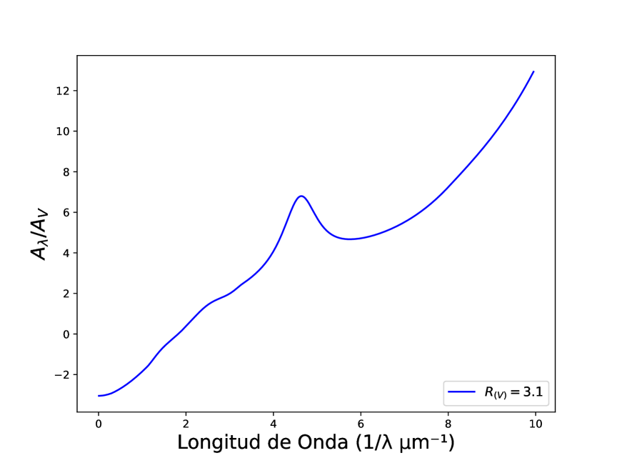
Figure 13: Extinction curve of $\mathrm{k(\lambda-V)}$ for wavelengths from $\mathrm{0.1\,\mu m^{-1}}$ to $\mathrm{160\,\mu m^{-1}}$.

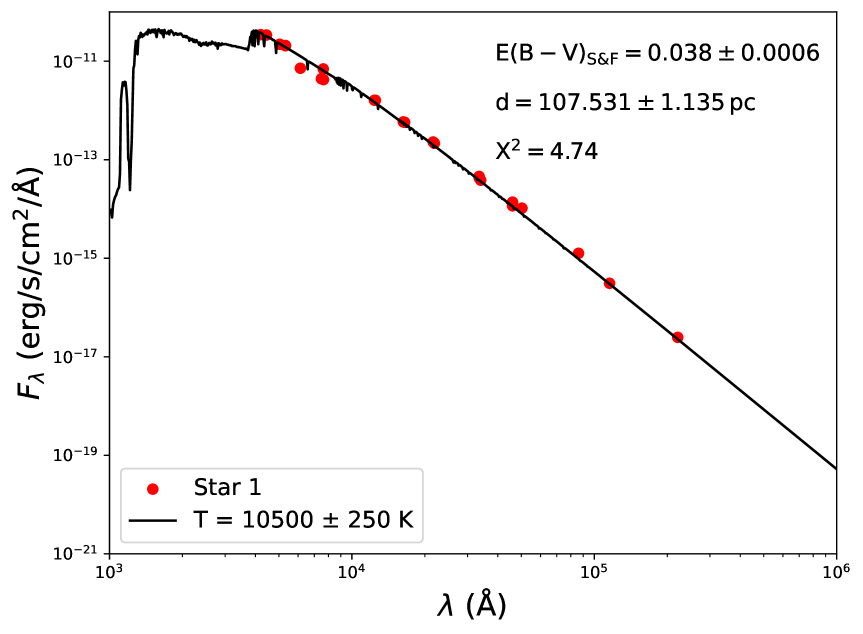
Figure 14: Theoretical SED spectral energy distribution for the star HD 72968, with the physical parameters of $\mathrm{T_{eff}=\rm{10500\pm 250\,K}}$, $\mathrm{logg=\rm{4.5\pm 0.5\,dex}}$, $\mathrm{R_{1}=2.5\pm 0.1\,R_{\odot}}$ y $\mathrm{d=107.531\pm 1.135\,pc}$

0.6 Conclusions

In this research work, a photometric and spectroscopic analysis was carried out for the chemically peculiar star HD 72968, where the following conclusions were made:

• For the photometric analysis, TESS (Transiting Exoplanet Survey Satellite) data were extracted, where the apparent magnitude of V = 5.6310 $\pm$ 0.0002 (mag) and the minimum magnitude of $m_{\mathrm{min}}$ = 5.6516 $\pm$ 0.0002 (mag) were obtained through the graphical representation of the magnitude histogram for HD 72968. Using the TESS data, the PDM-IRAF algorithm was implemented to determine the period of the star HD 72968, which resulted in P = 11.307 $\pm$ 0.005 d, and the value of the apparent minimum magnitude at the time BJD 2976.14736220 was confirmed.

• For a better graphical representation of the TESS photometric data, the wavelet data analysis technique was used, where we report a sub-period of 2.7 days possibly related to the star’s pulsations, which is approximately  76% shorter than the observed period of 11.307 d.

• We also identified changes in the morphology of the light curve at BJD=2976.15 and BJD=2963.31, where a sudden drop in the star’s brightness was observed, possibly related to some ejection of material caused by pulsation.

• From BJD=2963.31, it was observed that a disturbance in the light curve during the minimum is maintained, which is more extended and seems to be a remnant of the second eclipse or material ejection from the star.

• Additionally, an estimation of the effective temperature was made through the colorimetric method, which included a color-color plot of the J-H and H-K bands for 27 spectral type variants from O9 = 35900 K to K4 = 4560 K. The position of the star HD 72968 was identified with respect to other spectral types, obtaining the approximate effective temperature of 13550 $\pm$ 550 K, a value that shows significant variations compared to the real effective temperature values due to the comparison with main-sequence stars and the anomaly in its chemical composition for HD 72968.

• For the spectroscopic analysis, UVES spectra were obtained from the ESO (European Southern Observatory) database. Spectral treatments such as trimming, normalization, and Doppler effect correction were performed using the IRAF software. The identification of the main chemical elements present in HD 72968, such as Sr II, H $\mathrm{\delta}$, Cr II, and H $\mathrm{\beta}$, was carried out, each with its corresponding wavelength, spectral type, and equivalent width.

• For the chemical abundance analysis of HD 72968, the chemical elements and their atomic numbers were obtained from VizieR using the wavelengths of the main absorption lines. Subsequently, key parameters were determined using the NIST Atomic Spectra Database Lines Data to construct Table 6. Finally, the SPECTRUM ABUNDANCE software was used to identify the most abundant chemical elements in the star HD 72968, as presented in Figure 7.

• From the spectral analysis, a theoretical spectrum was generated using the SPECTRUM software, considering the ATLAS9 stellar atmosphere models over a wide range of temperatures from 7000 K to 15000 K. Using the chi-square statistical method, the best theoretical spectrum for HD 72968 was determined, obtaining the following parameters: $\mathrm{T_{eff}=10250\pm 250\,K}$, where the theoretical effective temperature value closely matches those determined by other authors over time, $\mathrm{logg=4.0\pm 0.5\,dex}$, $\mathrm{Vmicro=0.0\,kms^{-1}}$, $\mathrm{v_{sini}=8\pm 1\,kms^{-1}}$, $\mathrm{l/H}$ = 1.25, $\mathrm{M/H=0.00}$, and $\mathrm{\chi^{2}=18.5}$. It should be noted that the chi-square value was calculated entirely between the observed and theoretical spectrum for wavelengths from 4800 Å to 4900 Å.

• Additionally, a comparison was made between the star HD 72968 and chemically peculiar stars of similar spectral type, namely HD 220825 with $\mathrm{T_{eff}=9250K}$ and HD 223640 with $\mathrm{T_{eff}=12340K}$. The spectra were extracted from the ESO database, and the respective treatments of trimming, normalization with the IRAF Chebyshev function, and Doppler effect correction were applied. The spectral comparison between HD 72968 and HD 220825 yielded a chi-square value of $\mathrm{\chi^{2}=34.3}$, and the spectral comparison between HD 72968 and HD 223640 yielded a chi-square value of $\mathrm{\chi^{2}=66.1}$. Both values were used as upper and lower limits for estimating the effective temperature.

• A first spectral energy distribution (SED) was performed with the Kurucz ODFNEW / NOVER (2003) model in VOSA, obtaining the physical parameters for the star HD 72968: $\mathrm{T_{eff}=10000K}$, $\mathrm{logg=4.5\pm\,dex}$, $\mathrm{metallicity=0.5}$, $\mathrm{alpha=0.0}$, and $\mathrm{Av=0.195}$. Knowing the stellar parameters of HD 72968 and observing that the temperature obtained in VOSA falls within the range of the effective temperature determined from the theoretical spectrum, the theoretical effective temperature was calculated using the data obtained from the SED in VOSA with equation 8, yielding $\mathrm{T_{eff}=10000K}$.

• To determine the stellar radius of HD 72968, a theoretical spectral energy distribution (SED) was performed using the Kurucz ODFNEW / NOVER (2003) theoretical models from VOSA. Using equation 9, the total theoretical spectral flux for HD 72968 was determined for different wavelengths. Using the chi-square statistical method $\mathrm{\chi^{2}=4.744}$, the best theoretical model fitting the photometric data obtained from VIZIER-SED and spectroscopic analysis was determined, yielding the physical parameters, including the radius of HD 72968 in solar radii: $\mathrm{T_{eff}=10500\pm 250\,K}$, $\mathrm{logg=4.5\pm 0.5\,dex}$, stellar radius $\mathrm{R_{1}=2.5\pm 0.1\,R_{\mathrm{\odot}}}$, and $\mathrm{d=107.531\pm 1.135\,pc}$.

References

- Adelman (1998) Adelman S. J., 1998, A&AS, 128, 245. doi:10.1051/aas:1998138
- Adelman & Kaewkornmaung (2005) Adelman S. J., Kaewkornmaung P., 2005, A&A, 435, 1099. doi:10.1051/0004-6361:20042628
- Akeson & Christiansen (2019) Akeson R., Christiansen J., 2019, AAS
- Alan (2024) Alan N., 2024, NewA, 107, 102135. doi:10.1016/j.newast.2023.102135
- Auger & Tangborn (2004) Auger L., Tangborn A. V., 2004, MWRv, 132, 1220. doi:10.1175/1520-0493(2004)132<1220:AWRRKF>2.0.CO;2
- Babcock (1958) Babcock H. W., 1958, ApJ, 128, 228. doi:10.1086/146539
- Babcock (1958) Babcock H. W., 1958, ApJS, 3, 141. doi:10.1086/190035
- Bayo et al. (2008) Bayo A., Rodrigo C., Barrado Y Navascués D., Solano E., Gutiérrez R., Morales-Calderón M., Allard F., 2008, A&A, 492, 277. doi:10.1051/0004-6361:200810395
- Blackwell & Shallis (1977) Blackwell D. E., Shallis M. J., 1977, MNRAS, 180, 177. doi:10.1093/mnras/180.2.177
- Bessell & Brett (1988) Bessell M. S., Brett J. M., 1988, PASP, 100, 1134. doi:10.1086/132281
- Brandt (2021) Brandt T. D., 2021, ApJS, 254, 42. doi:10.3847/1538-4365/abf93c
- Castelli & Kurucz (2003) Castelli F., Kurucz R. L., 2003, IAUS, 210, A20. doi:10.48550/arXiv.astro-ph/0405087
- Castelli & Kurucz (2006) Castelli F., Kurucz R. L., 2006, A&A, 454, 333. doi:10.1051/0004-6361:20064999
- Catalano & Leone (1990) Catalano F. A., Leone F., 1990, A&AS, 83, 491
- Catalano, Renson, & Leone (1991) Catalano F. A., Renson P., Leone F., 1991, A&AS, 87, 59
- Catalano, Leone, & Kroll (1998) Catalano F. A., Leone F., Kroll R., 1998, A&AS, 129, 463. doi:10.1051/aas:1998199
- Cox (2000) Cox A. N., 2000, asqu.book
- Cardelli, Clayton, & Mathis (1989) Cardelli J. A., Clayton G. C., Mathis J. S., 1989, ApJ, 345, 245. doi:10.1086/167900
- Fitzpatrick & Massa (2005) Fitzpatrick E. L., Massa D., 2005, AJ, 130, 1127. doi:10.1086/431900
- Fuhrmann, Axer, & Gehren (1994) Fuhrmann K., Axer M., Gehren T., 1994, A&A, 285, 585
- Gaia Collaboration et al. (2018) Gaia Collaboration, Brown A. G. A., Vallenari A., Prusti T., de Bruijne J. H. J., Babusiaux C., Bailer-Jones C. A. L., et al., 2018, A&A, 616, A1. doi:10.1051/0004-6361/201833051
- Gaia Collaboration et al. (2018) Gaia Collaboration, Katz D., Antoja T., Romero-Gómez M., Drimmel R., Reylé C., Seabroke G. M., et al., 2018, A&A, 616, A11. doi:10.1051/0004-6361/201832865
- Heck, Mathys, & Manfroid (1987) Heck A., Mathys G., Manfroid J., 1987, A&AS, 70, 33
- Hensberge & De Loore (1974) Hensberge H., De Loore C., 1974, A&A, 37, 367
- Jaque et al. (2011) Jaque M., Fraga L., Paunzen E., Netopil M., 2011, BAAA, 54, 167
- Jaschek & Jaschek (1968) Jaschek C., Jaschek M., 1968, BAAA, 13, 13
- Jaschek & Jaschek (1968) Jaschek M., Jaschek C., 1968, BAAA, 11, 25
- Kunzli et al. (1997) Kunzli M., North P., Kurucz R. L., Nicolet B., 1997, A&AS, 122, 51. doi:10.1051/aas:1997291
- Lanz (1985) Lanz T., 1985, A&A, 144, 191
- Maury & Pickering (1897) Maury A. C., Pickering E. C., 1897, AnHar, 28, 1
- Morgan (1931) Morgan W. W., 1931, ApJ, 73, 104. doi:10.1086/143299
- Morgan (1933) Morgan W. W., 1933, PAAS, 7, 11
- Maitzen, Albrecht, & Heck (1978) Maitzen H. M., Albrecht R., Heck A., 1978, A&A, 62, 199
- Michaud (1970) Michaud G., 1970, ApJ, 160, 641. doi:10.1086/150459
- Megessier (1988) Megessier C., 1988, A&AS, 72, 551
- Morgan (1931) Morgan W. W., 1931, ApJ, 73, 104. doi:10.1086/143299
- Martin & Whittet (1990) Martin P. G., Whittet D. C. B., 1990, ApJ, 357, 113. doi:10.1086/168896
- Parenago (1958) Parenago P. P., 1958, SvA, 2, 151
- Paunzen (2004) Paunzen E., 2004, IAUS, 224, 443. doi:10.1017/S1743921304004867
- Preston (1971) Preston G. W., 1971, ApJ, 164, 309. doi:10.1086/150840
- Preston (1974) Preston G. W., 1974, ARA&A, 12, 257. doi:10.1146/annurev.aa.12.090174.001353
- Romanovskaya et al. (2021) Romanovskaya A. M., Shulyak D. V., Ryabchikova T. A., Sitnova T. M., 2021, A&A, 655, A106. doi:10.1051/0004-6361/202141740
- Rosales Guzmán et al. (2018) Rosales Guzmán J. A., Mennickent R. E., Djurašević G., Araya I., Curé M., 2018, MNRAS, 476, 3039. doi:10.1093/mnras/sty224
- Rosales et al. (2023) Rosales J. A., Mennickent R. E., Djurašević G., Araya I., Curé M., Schleicher D. R. G., Petrović J., 2023, A&A, 670, A94. doi:10.1051/0004-6361/202244046
- Smith (1996) Smith K. C., 1996, Ap&SS, 237, 77. doi:10.1007/BF02424427
- Stellingwerf (1978) Stellingwerf R. F., 1978, ApJ, 224, 953. doi:10.1086/156444
- Viswanath et al. (2023) Viswanath G., Janson M., Gratton R., Squicciarini V., Rodet L., Ringqvist S. C., Mamajek E. E., et al., 2023, A&A, 675, A54. doi:10.1051/0004-6361/202346154
- Wenger et al. (2000) Wenger M., Ochsenbein F., Egret D., Dubois P., Bonnarel F., Borde S., Genova F., et al., 2000, A&AS, 143, 9. doi:10.1051/aas:2000332
- Westendorp Plaza, Asensio Ramos, & Allende Prieto (2023) Westendorp Plaza C., Asensio Ramos A., Allende Prieto C., 2023, A&A, 675, A191. doi:10.1051/0004-6361/202346372
- Wright et al. (2010) Wright E. L., Eisenhardt P. R. M., Mainzer A. K., Ressler M. E., Cutri R. M., Jarrett T., Kirkpatrick J. D., et al., 2010, AJ, 140, 1868. doi:10.1088/0004-6256/140/6/1868