CubeDAgger: Improved Robustness of Interactive Imitation Learning without Violation of Dynamic Stability

Abstract

Interactive imitation learning makes an agent’s control policy robust by stepwise supervisions from an expert. The recent algorithms mostly employ expert-agent switching systems to reduce the expert’s burden by limitedly selecting the supervision timing. However, the precise selection is difficult and such a switching causes abrupt changes in actions, damaging the dynamic stability. This paper therefore proposes a novel method, so-called CubeDAgger, which improves robustness while reducing dynamic stability violations by making three improvements to a baseline method, EnsembleDAgger. The first improvement adds a regularization to explicitly activate the threshold for deciding the supervision timing. The second transforms the expert-agent switching system to an optimal consensus system of multiple action candidates. Third, autoregressive colored noise to the actions is introduced to make the stochastic exploration consistent over time. These improvements are verified by simulations, showing that the learned policies are sufficiently robust while maintaining dynamic stability during interaction.

I Introduction

Robots are expected to automatically perform a wide variety of tasks. The recent paradigm of training large models (i.e. control policies) by collecting a large set of demonstration datasets of tasks [1] can be considered a type of imitation learning [2], so the success of this approach is theoretically promised by minimizing approximation errors as much as possible. However, the costs of collecting data and learning grow as the system grows in size. Collecting enough datasets and acquiring compact policies is still useful in many domains (e.g. those where data is limited [3] and non-stationarity is strong [4]).

Interactive imitation learning (IIL) is a well-known methodology for improving policies by incrementally providing demonstration data [5]. In particular, dataset aggregation (DAgger) [6], which is the focus of this study, allows an agent and an expert to share control of a target robotic system. The expert takes the initiative at the beginning and gradually delegates control to the agent, who can complete the imitation without over- or under-learning. By introducing an appropriate safety criterion for delegating control, the expert can correct the robot to the optimal trajectory before it falls into a high-risk situation [7, 8, 9, 10]. Such a kind of error recovery motions can make the agent policy robust to accumulated approximation errors and/or disturbances.

However, recent DAgger variants have a method of discretely switching control authority, which causes two problems. First, if the expert is a human, he/she may not be able to respond immediately to the switching timing, resulting in a delay in the teaching operation [11]. Alternatively, if the switching timing is handled by him/her [7], the switching timing itself will be delayed. Another problem is that switching controllers is prone to cause discrete and abrupt changes in control commands to the robot, which could easily violate the stability of the robot [12]. Both of these problems can be ignored if the task is limited to (relatively) static manipulations, but in the case of dynamial systems, they easily violate dynamic stability in a synergistic manner.

To resolve this issue, this paper makes three improvements to EnsembleDAgger [8]. First, the agent policy is explicitly regularized so that it satisfies a specified level of safety for determining the control authority. Second, the switching system is replaced with an optimal consensus system of multiple action candidates. Finally, to facilitate more efficient exploration and increase robustness, time-consistent colored noise is injected into the agent’s actions, which is likely to make human decision-making less intractable.

The proposed method, so-called CubeDAgger, with these improvements is tested in three simulation environments with different dynamic characteristics. The results show that the proposed method improves the robustness of the learned policies over the conventional EnsembleDAgger without sacrificing dynamic stability during data collection.

I-A Related work

I-A1 DAgger family

DAgger [6] (and its variants [7, 8, 9, 10]) are representative of IIL. An agent and an expert share control of a target robotic system and combine each other’s actions appropriately to safely collect high-quality data. By including the expert’s actions rather than the actual actions into a dataset, the agent policy can asymptotically approach the expert one through supervised learning using it. Alternatively, the expert can improve the agent policy by only directing the agent to modify its actions.

In recent years, it has become common for the way actions are combined to be a switching system. The switching frequency that requires expert teaching is minimized, reducing the burden on the human expert [13, 14]. In this case, a single human operator can teach multiple robots simultaneously, facilitating data collection on a larger scale [15].

However, such an expert-agent switching system causes a delay between the switching of control authority and the correction by the human, and when the human makes the decision to switch control authority as well [7], limiting the target to systems in which the delay is ignorable [11]. In addition, switching systems would violate the stability of dynamic systems because of the discrete and abrupt changes in control commands to the robot [12]. In other words, this recent approach is inappropriate for IIL on dynamic systems.

I-A2 DART family

Another representative IIL methodology should be disturbances for augmenting robot trajectories (DART) [16]. This is a method in which the optimal (Gaussian) noise is injected into the expert’s actions when demonstrating a target task, increasing the uncertainty of state transitions and adding error recovery motions into the dataset. This noise optimization is extended to more flexible representation of policies by following Bayesian inference [17]. The various trajectories diversified by the added noise are ranked to extract the better ones to improve control performance [18].

However, as pointed out in the context of reinforcement learning (RL), stochastic exploration is inefficient [19]. The above DAgger is superior in terms of efficiency because it corresponds to directed exploration [20], although it is prone to exploration bias. Therefore, it is necessary to construct a system that takes advantage of both strengths.

I-A3 Integration with reinforcement learning

Although outside the scope of this study, several learning-from-demonstration methods utilizing RL have been proposed. Inverse RL [21] and guided RL [22] generally specify that the goal of RL is to increase similarity with demonstration data prepared offline, and scenarios in which the expert incrementally demonstrates the target task are rare. A method that interprets IIL as RL has emerged recently, outperforming the IIL baselines [23]. However, as it involves expert interventions by means of the switching system, it faces the same problem as the recent DAgger methods.

II Preliminaries

II-A Behavioral cloning

At first, behavioral cloning (BC) [2] is introduced since it is a main learning method of a agent’s policy even in IIL. Specifically, BC assumes that the target environment (i.e. a robot and surroundings) is Markovian, namely, the optimal policy, $\pi^{\ast}$, can be explained only with the current state observation, $s\in\mathcal{S}\subset\mathbb{R}^{|\mathcal{S}|}$, which is sampled according to the environment’s state transition probability (or its initial state probability) $p_{e}$. $\pi^{\ast}$ is hidden in an expert, but actions sampled from it at each state, $a\in\mathcal{A}\subset\mathbb{R}^{|\mathcal{A}|}$, can be collected. As a result, a dataset $D=\{(s_{n},a_{n})\}^{N}_{n=1}$ with $N$ pairs is prepared in advance.

The agent’s policy $\pi(a\mid s;\theta)$ with $\theta$ the trainable parameters is optimized towards $\pi^{\ast}$ by minimizing the following Kullback-Leibler divergence.

$$\theta^{\ast} =\mathop{\mathrm{arg\,min}}_{\theta}\underbrace{\mathbb{E}_{(s_{n},a_{n})\sim D}\left[-\ln\pi(a_{n}\mid s_{n};\theta)\right]}_{\mathcal{L}(\theta)}$$ (1)

where the expectation operation was approximated by sampling from $D$ generated from $p_{e}\pi^{\ast}$ by Monte Carlo method. The obtained loss function is minimized by, for example, stochastic gradient descent (e.g. AdaTerm [24] employed in this paper), to optimize $\theta$. Note that this study assumes that $\pi$ is a diagonal normal distribution with a learnable scale for continuous action space.

II-B Interactive imitation learning

In BC, $D$ is prepared and given in advance, but as shown in eq. (1), $D$ is intended to approximate the original expectation operation with $p_{e}\pi^{\ast}$. In other words, if $D$ is insufficient, the approximation error will be large and the imitation will fail eventually due to the accumulation of it. Therefore, IIL switches the BC’s problem setting to a new one that appends data into $D$ online, expecting that the policy trained becomes robust enough to the approximation error by collecting sufficient and necessary $D$.

However, to improve the value of expert data, how an agent would behave in the vicinity of an optimal trajectory (e.g. error recovery motions) is important. This reduces the approximation error efficiently and provide robustness to recover from deviations from the optimal trajectory due to the accumulation of errors. The pseudocode of DAgger family [6, 7, 8, 9, 10] with such a function is summarized in Alg. 1.

Algorithm 1 Pseudocode of DAgger family

1:Initialize network parameters $\theta$, and dataset $D=\emptyset$

2:while not converged do

3:  while not terminated or truncated do

4:   Get the current state $s$

5:   Get the expert’s action $a$ over $s$

6:   Get the agent’s action $a^{\pi}\sim\pi(a\mid s;\theta)$

7:   Determine the executed action $a^{c}$ from $a$ and $a^{\pi}$

8:   Transition to the next state using $a^{c}$

9:   Store experience $D=D\cup(s,a)$

10:  end while

11:  for $\{(s_{i},a_{i})\}_{i=1}^{B}\subset D$ do

12:   $\mathcal{L}(\theta)=-B^{-1}\sum_{i=1}^{B}\ln\pi(a_{i}\mid s_{i};\theta)$

13:   Minimize $\mathcal{L}(\theta)$ by stochastic gradient descent

14:  end for

15:end while

At Line 7 in Alg. 1, $a^{c}$, which actually acts on the environment, is determined based on $a$ demonstrated by the expert and $a^{\pi}$ of the agent. There is no unique solution for determining $a^{c}$, so several methods have been proposed in previous studies. In the original DAgger [6], the weighted average with annealing was employed. On the other hand, the recent trend is regarded as the following expert-agent switching system.

$$a^{c}=\begin{cases}a^{\pi}&(s,a^{\pi})\in\mathcal{C}\\ a&\mathrm{otherwise}\end{cases}$$ (2)

where, $\mathcal{C}$ denotes the safety set. That is, if the agent decision $a^{\pi}$ at the current state $s$ is safe, $a^{\pi}$ is accepted; otherwise, the expert should demonstrate the correct behaviors to make the environment with robot safe enough. The advantage of such a switching system is that the human expert does not need to demonstrate as long as the current situation is safe, and his/her burden can be greatly reduced, although this is not the case when $a$ is used to evaluate the safety. However, this paper does not focus on this advantage, but rather on solving the problems hidden in the switching system.

II-C EnsembleDAgger

As the baseline for the CubeDAgger proposed in the next section, EnsembleDAgger [8] is introduced here. In EnsembleDAgger, the agent evaluate the safety for switching $a$ and $a^{\pi}$, and the expert provides $a$ at evey time step, alleviating the delay of human decision making.

Specifically, EnsembleDAgger has $K$ ensembles of policies, $\{\pi_{k}(a\mid s;\theta_{k})\}_{k=1}^{K}$, each of which is trained with eq. (1). Therefore, the agent has $K$ action candidates, $\{a^{\pi_{k}}\}_{k=1}^{K}$, each of which is given as the location parameter of $\pi_{k}$ (without stochastic exploration) usually. At this time, not only $a^{\pi}=K^{-1}\sum_{k}a^{\pi_{k}}$ but also its standard deviation $\sigma^{\pi}=\sqrt{K^{-1}\sum_{k}(a^{\pi}-a^{\pi_{k}})^{2}}$ can be computed. EnsembleDAgger assumes that the current situation is safe if $a^{\pi}$ is close to $a$ and if $\sigma^{\pi}$ is enough small. With two thresholds, $\bar{\Delta}\geq 0$ and $\bar{\sigma}\geq 0$, the safety set, $\mathcal{C}$, is defined as follows:

$$\mathcal{C} =\{(s,a)\mid|a-a^{\pi}(s)|\leq\bar{\Delta}\land\sigma^{\pi}(s)\leq\bar{\sigma}\}$$ (3)

III Proposed method

III-A Overview

Since the current DAgger variants lack dynamic stability, the following three ‘C’ modifications are proposed as CubeDAgger to alleviate this issue.

1. Controlled: To reduce the hand-tuned $\mathcal{C}$ errors, the ensemble uncertainty is explicitly controlled to/under the specified thresholds.

2. Consensus: To effectively utilize the multiple action candidates of the ensemble model while eliminating abrupt changes in action due to the switching system, a consensus system is optimally designed.

3. Colored: To facilitate exploration while not interfering with the expert behaviors, autoregressive colored noise is introduced for time-consistent exploration.

III-B Controlled ensemble uncertainty

As mentioned above, EnsembleDAgger has $K$ policy ensemble models $\{\pi_{k}(a\mid s;\theta_{k})\}_{k=1}^{K}$, each of which is trained with eq. (1). Its basic idea is to have diverse inferenced outputs by taking advantage of the fact that $\theta_{k}$ are initialized differently, and to increase the accuracy of inference statistically. However, as it is, it is unknown to what extent the differences in output (represented by $\sigma^{\pi}=\sqrt{K^{-1}\sum_{k}(a^{\pi}-a^{\pi_{k}})^{2}}$ in EnsembleDAgger), even if the action space is pre-normalized well. As a result, the threshold $\bar{\sigma}$ for such an ensemble uncertainty is difficult to design in advance and tends to be the wrong $\mathcal{C}$.

III-B1 Formulation

Inspired by the literature [25], let’s consider controlling the ensemble uncertainty during learning. The proposed modification optimizes the ensemble models not only according to eq. (1), but also with the following inequality constraint on the ensemble uncertainty.

$$\ln(2\epsilon)\leq\max_{k}\ln(\bar{\sigma}^{-1}|a-a^{\pi_{k}}|+\epsilon)\leq\ln(1+\epsilon)$$ (4)

wherre, $\epsilon\ll 1$ denotes the tiny constant that is mainly used for numerical stabilization. This constraint prevents all $a^{\pi_{k}}$ from perfectly matching the expert’s action $a$, which would impair the statistical performance of the ensemble models, while the upper bound limits the deviation of any action candidate from $a$ to within the threshold. In other words, it is expected to reduce misjudgments of safety while ensuring the effectiveness of the ensemble models.

This inequality constraint is combined with eq. (1) by converting it to the corresponding regularization term [26]. In summary, the following loss function is minimized.

$$\mathcal{L}^{\mathrm{ctrl}}(\theta)\!=\!\mathbb{E}_{(s_{n},a_{n})\sim D}\!\Biggl{[}\! -\sum_{i=1}^{|\mathcal{A}|}\lambda_{i}\max_{k}\ln(\bar{\sigma}^{-1}|a_{i}-a_{i}^{\pi_{k}}|+\epsilon)$$

$$-\sum_{k=1}^{K}\ln\pi_{k}(a_{n}\mid s_{n};\theta_{k})\!\Biggr{]}$$ (5)

where, the subscript $i$ refers to the $i$-th dimension of action, and since the inequality constraint is given on each dimension independently, different Lagrange multipliers, $\lambda_{i}$, are provided for each. This implementation simplifies learning without the use of RL algorithms as in the literature [25].

III-B2 Optimization for satisfying inequality constraint

$\lambda$ can be optimized as Lagrange multipliers.

$$\phi_{\lambda}^{\ast} =\mathop{\mathrm{arg\,min}}_{\phi_{\lambda}}\underbrace{-\lambda(s_{n};\phi_{\lambda})e(a,a^{\pi},\delta)}_{\mathcal{L}^{\lambda}(\phi_{\lambda})}$$ (6)

$$e(a,a^{\pi},\delta) =\ln(2\epsilon)+\delta-\max_{k}\ln(\bar{\sigma}^{-1}|a-a^{\pi_{k}}|+\epsilon)$$

where, $\delta\in[0,\ln(1+\epsilon)-\ln(2\epsilon)]$ denotes the ($|\mathcal{A}|$-dimensional) slack variable to be optimized later. Since each state achieves the constraints differently, $\lambda$ is designed as a ($|\mathcal{A}|$-dimensional) state-dependent function with $\phi_{\lambda}$ the parameters accordingly.

Finally, the slack variable (the parameters of its state-dependent funciton, $\phi_{\delta}$) is optimized as follows to assist in satisfying the equality constraint [26].

$$\delta =g_{\delta}(\delta(s_{n};\phi_{\delta}))$$ (7)

$$\mathcal{L}^{\delta}(\phi_{\delta}) =\begin{cases}\delta(s_{n};\phi_{\delta})\mathrm{sign}(e(a,a^{\pi},\delta))&|e|>\bar{e}\\ \delta(s_{n};\phi_{\delta})\lambda&\mathrm{otherwise}\end{cases}$$ (8)

where, $g_{\delta}(\cdot)\in[0,\ln(1+\epsilon)-\ln(2\epsilon)]$ is the nonlinear transformation to satisfy the domain of the slack variable. $\bar{e}$ denotes the allowable error, and in this paper, it is designed as 10 % of the domain size. If $e\leq\bar{e}$, the position of equality constraint is shifted towards the lower or upper bound of $\delta$ according to $\lambda$: if $\lambda>0$ to maximize the ensemble uncertainty, its behavior is suppressed by making $\delta$ small, and vice versa. This behavior allows the change in the ensemble uncertainty to be stably controlled while simultaneously searching for solutions that may lie at both boundaries of the inequality constraint.

III-C Consensus system among ensemble actions

Recent DAgger variant, such as EnsembleDAgger, use a safety-based switching system to decide which action $a^{c}$ to execute from the expert’s action candidate $a$ and the agent’s action candidate $a^{\pi}$. However, as mentioned above, safety decisions left to human are subject to delay, and switching can cause abrupt changes in robot’s commands, which can violate the stability of the dynamic system. Therefore, this study considers the decision of $a^{c}$ as a kind of consensus-making problem in which a central tendency is derived from multiple candidates, and designs a system that can obtain an optimal consensus with safety taken into account.

III-C1 Formulation

The consensus-making problem of deriving $a^{c}$ is regarded as the central tendency of multiple action candidates, i.e. $a^{\pi_{k}}$ ($k=1,\ldots,K$) of the agent and $a$ of the expert. This can be attributed to the $L_{p}$ norm minimization problem for the $i$-th action dimension as shown below [27].

$$a_{i}^{c}=\mathop{\mathrm{arg\,min}}_{c_{i}\in[\underline{a}_{i},\overline{a}_{i}]}\left\{\sum_{k=1}^{K}w_{k}|a_{i}^{\pi_{k}}-c_{i}|^{p_{i}}+w_{K+1}|a_{i}-c_{i}|^{p_{i}}\right\}^{\frac{1}{p_{i}}}$$ (9)

where, $\underline{a}_{i}$ and $\overline{a}_{i}$ denote the minimum and maximum values among the candidates, respectively. $w_{k}$ is the weigtht for $k$-th candidate, the sum of which satisfies $1$. Note that when $a^{c}$ is inferred only by agents (especially after deployment), the $K+1$-th candidate for $a$ is merely excluded.

With $p_{i}>1$, $L_{p_{i}}$ norm becomes strictly convex, the global optimum is obtained fast and asymptotically. However, when $p_{i}$ is very large, Newton methods that require (pseudo-)quadratic gradients become unstable numerically. Therefore, it is converted to the corresponding root-finding problem for its analytical first-order gradient, which can be asymptotically solved by a kind of bisection methods, so that the numerical stability of the solution is guaranteed. In practice, ITP method [28], which has theoretically shown fast convergence, has been employed in this study.

$a_{i}^{c}$ obtained by solving such a problem has different properties according to $p_{i}$ and $w_{k}$. Here, $w_{k}$ is ignored at once for simplicity, and three representative results are summarized as below.

• $p_{i}\to 1$: This yields the median, which can elimiate outliers mixed in with the candidates, $\mathrm{Quantile(\{a_{i}^{\pi_{k}}\}_{k=1}^{K}\cup\{a\};0.5)}$.

• $p_{i}=2$: This yields the mean, which is the fairest central tendency if the candiates are distributed as Gaussian, $(K+1)^{-1}(\sum_{k=1}^{K}a_{i}^{\pi_{k}}+a)$.

• $p_{i}\to\infty$: This yields the midrange, which is the fairest central tendency if the candidates are distributed uniformly, $(\underline{a}_{i}+\overline{a}_{i})/2$.

Note that the intermediate $p_{i}$ has a mixture of these properties. As the consensus should be fair while anomalous opinions should be excluded, it is worth desigining the proper $p_{i}$ according to the distribution shape of candidates.

The above properties are the same even when $w_{k}$ is included, since it only vary the number of pseudo-candidates. Thus, given appropriate weights, the conventional discrete switching system can be extended to a continuous one.

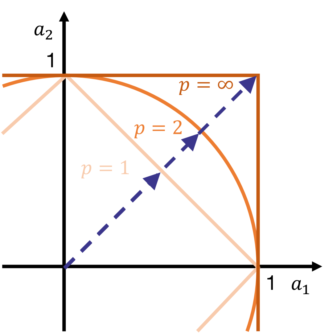
(a) Geometry of $L_{p}$ norm

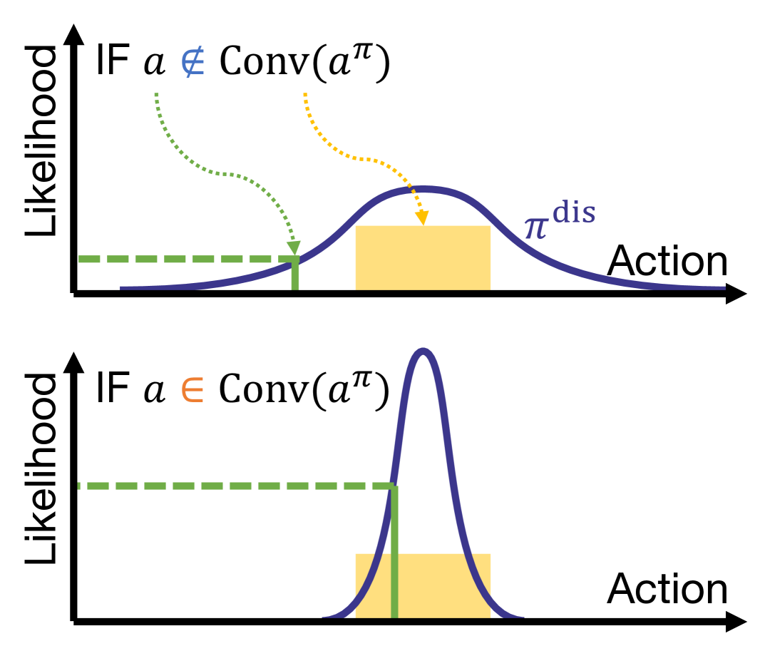
(b) Geometry of actions

Figure 1: Geometries for designing $p_{i}$ and $w_{k}$

III-C2 Design of $p_{i}$

To determine $p_{i}$, the distribution shape should be quantified, as indicated above. For this purpose, the ratio of the standard deviation, $\sigma_{i}^{\mathrm{STD}}$, and mean absolute error, $\sigma_{i}^{\mathrm{MAE}}$, for the candidates is defined as $\rho_{i}$.

$$\rho_{i} =\cfrac{\sigma_{i}^{\mathrm{MAE}}}{\sigma_{i}^{\mathrm{STD}}}$$ (10)

$$\mathrm{s.t.\ } \begin{cases}\sigma_{i}^{\mathrm{STD}}=\sqrt{\sum_{k=1}^{K}w_{k}(\mu_{i}-a_{i}^{\pi_{k}})^{2}+w_{K+1}(\mu_{i}-a_{i})^{2}}\\ \sigma_{i}^{\mathrm{MAE}}=\sum_{k=1}^{K}w_{k}|\mu_{i}-a_{i}^{\pi_{k}}|+w_{K+1}|\mu_{i}-a_{i}|\\ \mu_{i}\ \ \ \ =\sum_{k=1}^{K}w_{k}a_{i}^{\pi_{k}}+w_{K+1}a_{i}\end{cases}$$

This ratio is known to be $\sqrt{2/\pi}(\simeq 0.8)$ if the candidates follow a Gaussian distribution. If the candidates follow a uniform distribution, it asymptotically approaches $1$, and if they are non-Gaussian, such as heavily tailed and/or asymmetric, it approaches $0$. Therefore, $p_{i}$ can be defined as the function of $\rho_{i}$. However, since $p_{i}$ and $\rho_{i}$ have different domains, a reasonable connection between them is required.

This paper focuses on the longest distance $d_{i}$ from the origin among sets in a $K+1$-dimensional space where the $L_{p_{i}}$ norm is $1$ (see Fig. 1(a)). Three important cases are as follows: $\sqrt{K+1}^{-1}$ for $p_{i}\to 1$; $1=\sqrt{K+1}^{0}$ for $p_{i}=2$; and $\sqrt{K+1}^{1}$ for $p_{i}\to\infty$. Here, the power part (defined as $q_{i}$) is bounded by $(-1,1)$, and the connection with $\rho_{i}$ can be easily made by the following equation.

$$d_{i}=\sqrt{K+1}^{q_{i}}=2\rho_{i}^{\frac{\ln 2}{\ln\sqrt{\pi/2}}}-1$$ (11)

Then, the coordinates in the $K+1$-dimensional space with $d_{i}$ have the same values on all axes, i.e. $d_{i}/\sqrt{K+1}=\sqrt{K+1}^{q_{i}-1}$. With one $L_{p_{i}}$ norm, $p_{i}$ is derived as follows:

$$(K+1)\left(\sqrt{K+1}^{q_{i}-1}\right)^{p_{i}}=1$$

$$\therefore\ p_{i}=\frac{1}{1-\rho_{i}^{\frac{\ln 2}{\ln\sqrt{\pi/2}}}}$$ (12)

III-C3 Design of $w_{k}$

The weight $w_{k}$ ($k=1,\ldots,K+1$) for each candidate is designed. Each candidate is generated from the corresponding policy $\pi_{k}$, and its likelihood can be taken as the confidence level. However, this likelihood is quantifiable only for the agent actions, and cannot be numerically calculated for the expert because $\pi^{\ast}$ is unknown. While there may be a direction to receive information equivalent to the likelihood from the expert, or to estimate it, this paper utilizes the safety definition in EnsembleDAgger.

As one of the safety with the threshold $\bar{\sigma}$ for the ensemble uncertainty, an alternative policy $\pi^{\mathrm{exp}}$ to $\pi^{\ast}$ is assumed with a diagonal normal distribution with $a$ the mean and $\bar{\sigma}/3$ the scale parameters. This means that the likelihood of $\pi_{k}$ is essentially smaller than that of $\pi^{\mathrm{exp}}$ unless the ensemble uncertainty is controlled to be below the threshold and the scale of $\pi_{k}$ is correspondingly smaller, resulting in a preference for the expert’s action $a$. Another safety is that the difference between $a$ and $\mu^{\pi}=K^{-1}\sum_{k=1}^{K}a^{\pi_{k}}$ should be below a threshold. This can be represented with another diagonal normal distribution with $\mu^{\pi}$ the mean and the mean squared error of $a$ and $a^{\pi_{k}}$ as its variance, $\pi^{\mathrm{dis}}$ (see Fig. 1(b)). That is, if the likelihood of $a$ of $\pi^{\mathrm{dis}}$ is large, the agent would be similar to the expert and safe. Note that $\bar{\Delta}$ in EnsembleDAgger is not needed since $\pi^{\mathrm{dis}}$ makes it easier to confirm whether $a$ is contained inside the convex hull given by $a^{\pi_{k}}$, leading to $a^{c}\simeq a$ even without $a$.

Finally, the weight $w_{k}$ is designed as follows:

$$w_{k}\propto\begin{cases}\cfrac{\pi^{\mathrm{exp}}(a\mid a,\bar{\sigma}/3)}{\pi^{\mathrm{dis}}(a\mid\mu^{\pi},\sqrt{K^{-1}\sum_{k=1}^{K}(a-a^{\pi_{k}})^{2}})}&k=K+1\\ \pi_{k}(a^{\pi_{k}}\mid s;\theta_{k})&\mathrm{otherwise}\end{cases}$$ (13)

Note that $w_{k}$ is normalized to sum to $1$ to satisfy its definition. Thanks to this design, it allows for safety considerations analogous to EnsembleDAgger, while obtaining continuous $a^{c}$ decisions than simple switching systems.

III-D Colored noise for time-consistent exploration

In the context of RL, action noise from the stochastic policy is effective, and DART variants [16, 17], another approach to IIL, make the learned policy robust by adding optimized noise to the expert’s behavior. Thus, the exploration noise is also considered effective even in DAgger variants. In the above research cases (with continuous action space), however, the exploration noise is white noise generated from a Gaussian distribution. In other words, noise is time-independent, and a robot system fastly oscillated by it might be difficult for a human expert to operate.

Therefore, this study employes colored noise, which has been reported to accelerate exploration rather than white one, inspired by the literature [29]. However, previous studies have used an implementation that generates time-series noises with a specified time step in advance, perhaps in order to investigate general colored noise, which is not flexible enough in practice. Red noise is therefore selected since it can be generated with an autoregressive model as follows:

$$\epsilon^{\mathrm{red}}_{t}=\gamma\epsilon^{\mathrm{red}}_{t-1}+\sqrt{1-\gamma^{2}}\epsilon^{\mathrm{white}}_{t}$$ (14)

where $\epsilon^{\mathrm{red}}_{0}=\epsilon^{\mathrm{white}}_{0}$. $\gamma\in[0,1)$ represents the temporal consistency, and is given as $\exp(-\Delta t/T)$ with $\Delta t$ the time step period and $T$ the time constant (see Fig. 2).

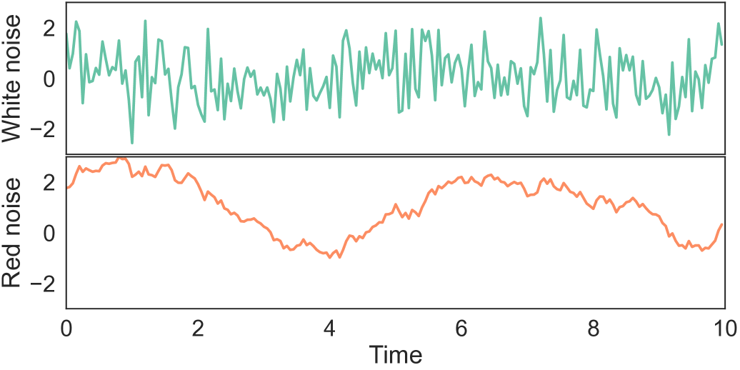
Figure 2: Time consistency of red noise ($\Delta t=0.05$ and $T=3$)

To add the red noise into the agent’s actions, the likelihood (a.k.a. confidence for computing $w_{k}$) needs to be taken into account. That is, the excessive red noise to prioritize exploration would make the likelihood smaller than others (especially the expert’s one), losing the chance of reflecting it to $a^{c}$. With this in mind, $a^{\pi}$ is finally given as follows:

$$a^{\pi}=\mu_{\pi}+\cfrac{2\sqrt{K}}{3}\sigma_{\pi}\epsilon^{\mathrm{red}}_{t}$$ (15)

where, $\mu_{\pi}$ and $\sigma_{\pi}$ denote the mean and scale of $\pi$, which is modeled as a diagonal normal distribution, respectively. Note that $\epsilon^{\mathrm{red}}_{t}$ is different for each dimension of the action space and for each component of the ensemble model. As white and red noises are generally within $\pm 2\sim 3$, this gain, $2\sqrt{K}/3$, increases the expert’s confidence level relatively only to $K\sim 2K$, even if all components carry the maximum amount of exploration noise. In other words, the difference of the number of candidates from the agent and expert is compensated with this design, and the actions from the agent are possibly reflected into $a^{c}$ (depending on $p_{i}$ and $w_{k}$).

IV Simulations

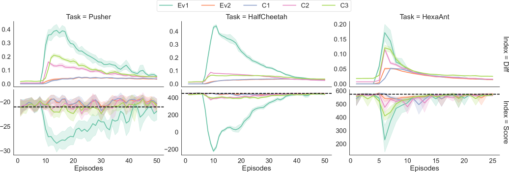
Figure 3: Trajectories during data collection (dashed lines: the experts’ average scores)

In order to statistically verify the performance of the proposed method, CubeDAgger, the following simulations are conducted. The important criteria are threefold: i) the difference between the expert’s action $a$ and the executed action $a^{c}$ during the data collection process; ii) the degree of degradation of control performance during the data collection process; iii) the robustness of the learned policies.

IV-A Tasks

Three tasks with different robots simulated in Mujoco are performed. The first Pusher, where a manipulator pushes an object to its destination without grasping it, might cause the object to slide into hard-to-push positions by wrong actions. The second HalfCheetah, where a 2D legged robot moves forward while standing on its head, is unstable and sensitive to mistakes. The third HexaAnt, which has a multi-degree-of-freedom system with three joints in each of its six legs for walking foward, is easy to intervene in state transitions and stability with various action patterns. These tasks were trained multiple times with the RL algorithm [30], and the best policies are selected as their experts. Since the experts maximized the sum of rewards, the control performance is evaluated by it.

IV-B Models

The policy of the imitation agent is approximated by neural networks with two fully-connected layers (each with 100 neurons) in the hidden layer. To make it a lightweight ensemble model, only the output layer is separated to take $K=10$ outputs (i.e. the mean and log scale of Gaussian distribution), while sharing the input and hidden layers [31]. This policy ensembles (and other learnable parameters) are optimized using AdaTerm [24], a stochastic gradient descent method that is robust to noise and outliers. The dataset $D$ is assumed to have the sufficient capacity to hold all the data during the experiments, and all the data in $D$ are uniformly randomly replayed once at the end of each episode with batch size $B=50$ each.

IV-C Comparisons

The following five conditions including ablation tests are compared.

• EV1: EnsembleDAgger with (almost) recommended configurations, i.e. $\bar{\Delta}=1$ and $\bar{\sigma}=0.1$.

• EV2: EnsembleDAgger that eliminates $\bar{\Delta}$ as in the proposed method, $\bar{\Delta}=0.1$ and $\bar{\sigma}=0.1$.

• C1: EV2 with the controlled ensemble uncertainty.

• C2: C1 with the consensus system.

• C3: The proposed method with all the modifications including the colored noise (a.k.a. CubeDAgger).

Here, for fair comparison, the same threshold value of $\bar{\sigma}=0.1$ is used for C1, C2, and C3.

IV-D Results

The difference $|a-a^{c}|$ (labeled Diff) and the sum of rewards (labeled Score) at the time of data collection are plotted in Fig. 3. Apparently, EV1 frequently performed actions different from those of the experts, causing large drops in the scores. This behavior would involve significant risk during data collection in real-world robot applications, even if it is needed to learn how to recover from (accumulated) errors in case of failure. On the other hand, EV2 mostly prioritized $a$ for determining $a^{c}$, and the scores were always high. In other words, this behavior suggests a lack of exploration, although this will be evident later when we look at the behavior of the learned policies.

Focusing on the proposed modifications, C1 did not change much from EV2, except for a slight delay in the timing at which $|a-a^{c}|$ began to grow. On the other hand, the behavior of C2 was clearly different, and its exploratory behavior was between those of EV1 and EV2. The fact that the score did not decrease much suggests that the consensus was gained more safely than the case with EnsembleDAgger (i.e. the simple if-then rule). In addition, although $|a-a^{c}|$ should become smaller as the episodes pass due to the convergence of the agent policy to the expert’s one, C3 made it remain for longer period thanks to the colored noise moderately added. The noise also caused a slight decrease in the score, but not as much as in the case of EV1.

To compare the five methods more quantitatively, two criteria are statistically evaluated. The one shows the ability to maintain the control performance during data collection, labeled Retention, which is computed as the mean of scores during data collection. The other shows the robustness of the learned policies, labeled Robustness, which is evaluated by deploying them under the disturbed environments, where a uniform random disturbance with a probability of 5 % to each action dimension. Note that the maximum intensity of the disturbance was set to the largest action of each dimension for Pusher and HexaAnt, and to the half of it for HalfCheetah due to its instability.

The normalized results of both criteria are summarized in Fig. 4. As the learning process already suggested, EV1 caused a significant performance degradation, while EV2 almost maintained the expert’s control performance. Although the control performance degraded with each proposed modification, it rarely exceeded the worst case of experts (given as the dashed lines). It would simply be expected that the robustness should be inversely proportional to the retention, and this is the case when looking at EV1 and EV2. However, with the similar retention to EV2, C1 was clearly more robust. More surprisingly, C2, which has the better retention than EV1, achieved the same level of robustness, and C3 achieved even better robustness. This indicates that the proposed CubeDAgger could more efficiently facilitate the exploration to improve the robustness.

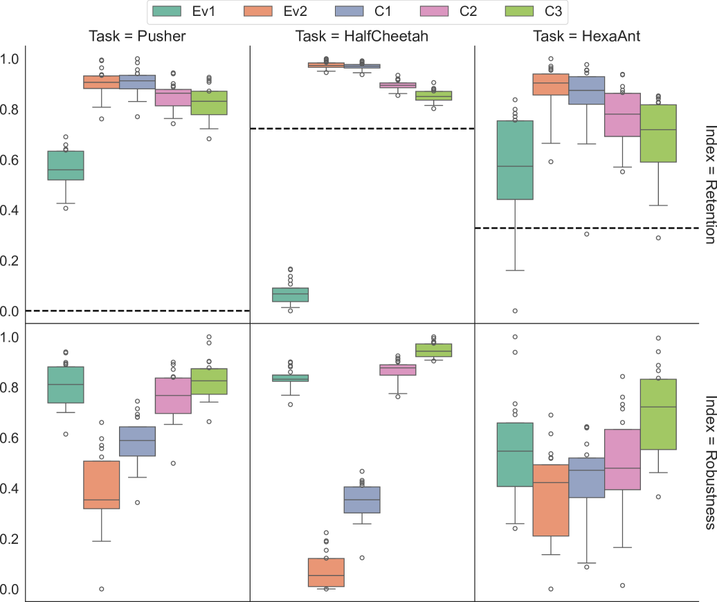
Figure 4: Statistical evaluation with 21 random seeds for each condition (dashed lines: the experts’ worst-case scores)

V Conclusion

This paper proposed a novel IIL method, named CubeDAgger, an improved version of EnsembleDAgger. The improvements are threefold: i) control the output variance of the ensemble model to make the safety decision work better; ii) design an optimization problem to derive consensus from multiple action candidates; and iii) add colored noise for efficient probabilistic exploration. With these improvements, CubeDAgger successfully improved the robustness of learned policies while maintaining dynamic stability during data collection, compared to EnsembleDAgger. Future work will demonstrate the practicality of CubeDAgger through real-world robot experiments and verify that the colored noise is less disruptive to human demonstrations than ordinary white noise.

References

- [1] K. Kawaharazuka, T. Matsushima, A. Gambardella, J. Guo, C. Paxton, and A. Zeng, “Real-world robot applications of foundation models: A review,” Advanced Robotics, vol. 38, no. 18, pp. 1232–1254, 2024.
- [2] M. Bain and C. Sammut, “A framework for behavioural cloning.” in Machine Intelligence 15, 1995, pp. 103–129.
- [3] R. Mori, T. Aoyama, T. Kobayashi, K. Sakamoto, M. Takeuchi, and Y. Hasegawa, “Real-time spatiotemporal assistance for micromanipulation using imitation learning,” IEEE Robotics and Automation Letters, vol. 9, no. 4, pp. 3506–3513, 2024.
- [4] E. Johns, “Coarse-to-fine imitation learning: Robot manipulation from a single demonstration,” in IEEE international conference on robotics and automation. IEEE, 2021, pp. 4613–4619.
- [5] C. Celemin, R. Pérez-Dattari, E. Chisari, G. Franzese, L. de Souza Rosa, R. Prakash, Z. Ajanović, M. Ferraz, A. Valada, J. Kober, et al., “Interactive imitation learning in robotics: A survey,” Foundations and Trends® in Robotics, vol. 10, no. 1-2, pp. 1–197, 2022.
- [6] S. Ross, G. Gordon, and D. Bagnell, “A reduction of imitation learning and structured prediction to no-regret online learning,” in International Conference on Artificial Intelligence and Statistics. JMLR Workshop and Conference Proceedings, 2011, pp. 627–635.
- [7] M. Kelly, C. Sidrane, K. Driggs-Campbell, and M. J. Kochenderfer, “Hg-dagger: Interactive imitation learning with human experts,” in International Conference on Robotics and Automation. IEEE, 2019, pp. 8077–8083.
- [8] K. Menda, K. Driggs-Campbell, and M. J. Kochenderfer, “Ensembledagger: A bayesian approach to safe imitation learning,” in IEEE/RSJ International Conference on Intelligent Robots and Systems. IEEE, 2019, pp. 5041–5048.
- [9] Y. Cui, D. Isele, S. Niekum, and K. Fujimura, “Uncertainty-aware data aggregation for deep imitation learning,” in International Conference on Robotics and Automation. IEEE, 2019, pp. 761–767.
- [10] H. Oh and T. Matsubara, “Leveraging demonstrator-perceived precision for safe interactive imitation learning of clearance-limited tasks,” IEEE Robotics and Automation Letters, vol. 9, no. 4, pp. 3387–3394, 2024.
- [11] D. G. Black, D. Andjelic, and S. E. Salcudean, “Evaluation of communication and human response latency for (human) teleoperation,” IEEE Transactions on Medical Robotics and Bionics, vol. 6, no. 1, pp. 53–63, 2024.
- [12] D. Liberzon and A. S. Morse, “Basic problems in stability and design of switched systems,” IEEE control systems magazine, vol. 19, no. 5, pp. 59–70, 1999.
- [13] R. Hoque, A. Balakrishna, C. Putterman, M. Luo, D. S. Brown, D. Seita, B. Thananjeyan, E. Novoseller, and K. Goldberg, “Lazydagger: Reducing context switching in interactive imitation learning,” in IEEE international conference on automation science and engineering. IEEE, 2021, pp. 502–509.
- [14] R. Hoque, A. Balakrishna, E. Novoseller, A. Wilcox, D. S. Brown, and K. Goldberg, “Thriftydagger: Budget-aware novelty and risk gating for interactive imitation learning,” in Conference on Robot Learning. PMLR, 2022, pp. 598–608.
- [15] R. Hoque, L. Y. Chen, S. Sharma, K. Dharmarajan, B. Thananjeyan, P. Abbeel, and K. Goldberg, “Fleet-dagger: Interactive robot fleet learning with scalable human supervision,” in Conference on Robot Learning. PMLR, 2023, pp. 368–380.
- [16] M. Laskey, J. Lee, R. Fox, A. Dragan, and K. Goldberg, “Dart: Noise injection for robust imitation learning,” in Conference on robot learning. PMLR, 2017, pp. 143–156.
- [17] H. Oh, H. Sasaki, B. Michael, and T. Matsubara, “Bayesian disturbance injection: Robust imitation learning of flexible policies for robot manipulation,” Neural Networks, vol. 158, pp. 42–58, 2023.
- [18] D. S. Brown, W. Goo, and S. Niekum, “Better-than-demonstrator imitation learning via automatically-ranked demonstrations,” in Conference on robot learning. PMLR, 2020, pp. 330–359.
- [19] R. S. Sutton and A. G. Barto, Reinforcement learning: An introduction. MIT press, 2018.
- [20] R. C. Wilson, E. Bonawitz, V. D. Costa, and R. B. Ebitz, “Balancing exploration and exploitation with information and randomization,” Current opinion in behavioral sciences, vol. 38, pp. 49–56, 2021.
- [21] S. Adams, T. Cody, and P. A. Beling, “A survey of inverse reinforcement learning,” Artificial Intelligence Review, vol. 55, no. 6, pp. 4307–4346, 2022.
- [22] J. Eßer, N. Bach, C. Jestel, O. Urbann, and S. Kerner, “Guided reinforcement learning: A review and evaluation for efficient and effective real-world robotics [survey],” IEEE Robotics & Automation Magazine, vol. 30, no. 2, pp. 67–85, 2022.
- [23] J. Luo, P. Dong, Y. Zhai, Y. Ma, and S. Levine, “Rlif: Interactive imitation learning as reinforcement learning,” in International Conference on Learning Representations, 2024.
- [24] W. E. L. Ilboudo, T. Kobayashi, and T. Matsubara, “Adaterm: Adaptive t-distribution estimated robust moments for noise-robust stochastic gradient optimization,” Neurocomputing, vol. 557, p. 126692, 2023.
- [25] K. Brantley, W. Sun, and M. Henaff, “Disagreement-regularized imitation learning,” in International Conference on Learning Representations, 2020.
- [26] T. Kobayashi, “Lira: Light-robust adversary for model-based reinforcement learning in real world,” arXiv preprint arXiv:2409.19617, 2024.
- [27] M. Chavent and J. Saracco, “On central tendency and dispersion measures for intervals and hypercubes,” Communications in Statistics—Theory and Methods, vol. 37, no. 9, pp. 1471–1482, 2008.
- [28] I. F. Oliveira and R. H. Takahashi, “An enhancement of the bisection method average performance preserving minmax optimality,” ACM Transactions on Mathematical Software, vol. 47, no. 1, pp. 1–24, 2021.
- [29] O. Eberhard, J. Hollenstein, C. Pinneri, and G. Martius, “Pink noise is all you need: Colored noise exploration in deep reinforcement learning,” in The Eleventh International Conference on Learning Representations, 2023.
- [30] T. Kobayashi, “Revisiting experience replayable conditions,” Applied Intelligence, vol. 54, no. 19, pp. 9381–9394, 2024.
- [31] I. Osband, C. Blundell, A. Pritzel, and B. Van Roy, “Deep exploration via bootstrapped dqn,” Advances in neural information processing systems, vol. 29, 2016.