Model selection for unit-root time series with many predictors

Supplement for “Model Selection for Unit-root Time Series with Many Predictors”

Abstract

This paper studies model selection for general unit-root time series, including the case with many exogenous predictors. We propose FHTD, a new model selection algorithm that leverages forward stepwise regression (FSR), a high-dimensional information criterion (HDIC), a backward elimination method based on HDIC, and a data-driven thresholding (DDT) approach. Under some mild assumptions that allow for unknown locations and multiplicities of the characteristic roots on the unit circle of the time series and conditional heteroscedasticity in the predictors and errors, we establish the sure screening property of FSR and the selection consistency of FHTD. Central to our analysis are two key technical contributions, a new functional central limit theorem for multivariate linear processes and a uniform lower bound for the minimum eigenvalue of the sample covariance matrices, both of which are of independent interest. Simulation results corroborate the theoretical properties and show the superior performance of FHTD in model selection. We showcase the application of the proposed FHTD by modeling U.S. monthly housing starts and unemployment data.

1 Introduction

With the widespread availability of large-scale fine-grained datasets, researchers analyzing time series data now have a plethora of predictors available for constructing informative and interpretable models. Regularization techniques (Tibshirani, 1996; Zou, 2006; Candes and Tao, 2007; Zhang, 2010; Zheng, Fan and Lv, 2014), which select a few relevant features in a sparse model for prediction, have thus been adapted from the independent framework to time series data (Medeiros and Mendes, 2016; Han and Tsay, 2020). In addition, greedy forward selection algorithms (Bühlmann, 2006; Wang, 2009; Fan and Lv, 2008; Ing and Lai, 2011) have also proven useful for a similar task involving dependent data (Ing, 2020).

However, the aforementioned methods are generally not applicable to unit-root nonstationary time series, prevalent in economics, finance, and environmental sciences. To apply these methods to unit-root time series, one must carefully transform the series under study into stationary ones. This step often involves multiple intricate unit-root tests since the underlying unit-root structure is typically unknown. In addition, it becomes even more challenging to take the correct difference transforms when the data are driven by complex unit roots, such as those exhibiting persistent cyclic behavior. Determining the order of integration and the frequency at which the series is integrated are far from straightforward and are sometimes sensitive to model specifications. Yet, persistent cyclic (or seasonal) time series are widely encountered in applications, such as the unemployment rate (Bierens, 2001), spot exchange rates (Al-Zoubi, 2008), entrepreneurship series (Faria, Cuestas and Gil-Alana, 2009), firms’ capital structure (Al-Zoubi, O’Sullivan and Alwathnani, 2018), sunspot numbers (Gil-Alana, 2009; Maddanu and Proietti, 2022), oil prices (Gil-Alana and Gupta, 2014), tourist arrivals (del Barrio Castro, Cubadda and Osborn, 2022), and CO₂ concentrations (Proietti and Maddanu, 2024), to name just a few examples.

In this paper, we study model selection for an autoregressive model with exogenous variables, known as the ARX model, when the dependent variable contains general unit roots and the number of exogenous variables is large. Specifically, the model employed is

$$(1-B)^{a}(1+B)^{b}\prod_{k=1}^{l}(1-2\cos\vartheta_{k}B+B^{2})^{d_{k}}\psi_{n}(B)y_{t,n}=\sum_{j=1}^{p_{n}}\sum_{l=1}^{r_{j}^{(n)}}\beta_{l,n}^{(j)}x_{t-l,j}^{(n)}+\epsilon_{t,n},$$ (1)

$t=1,\ldots,n$, where $n$ is the sample size, $B$ denotes the back-shift operator, $a$, $b$, and $d_{k}$ are nonnegative integers indicating the order of integration with respect to different (conjugate) unit roots, $l$ is the number of complex conjugate unit-root pairs, $\vartheta_{k}\in(0,\pi)$ denotes the location of a complex unit root, and $\psi_{n}(z)=1+\sum_{s=1}^{\iota_{n}}a_{s,n}z^{s}\neq 0$ for all $|z|\leq 1$, with both $a_{s,n}\in\mathbb{R}$ and $\iota_{n}\in\mathbb{N}\cup\{0\}$ unknown. In particular, we assume no prior knowledge about the unit roots in the model, so $a$, $b$, $l$, $d_{k}$ and $\vartheta_{k}$ are all unknown. In model (1), $\{\epsilon_{t,n}\}$ denotes a sequence of random errors with mean zero, $\{x_{t-l,j}^{(n)}\}$ and $\{\beta_{l,n}^{(j)}\}$, for $1\leq l\leq r_{j}^{(n)},1\leq j\leq p_{n}$, are observable exogenous variables and their respective unknown coefficients. Let $d=a+b+2\sum_{k=1}^{l}d_{k}$. The number of AR lags in (1), $m_{n}=\iota_{n}+d$, is assumed to be smaller than $n$, whereas the number of exogenous predictors, $p_{n}^{*}=\sum_{j=1}^{p_{n}}r_{j}^{(n)},$ can be much greater than $n$. We adopt $y_{t,n}=0$ for $t\leq 0$ as the initial conditions, which are widely used in the literature for unit-root series (e.g. Chan and Wei, 1988). Last but not least, we allow $\{x_{t,j}^{(n)},1\leq t\leq n\}$, for $1\leq j\leq p_{n}$, and $\{\epsilon_{t,n}\}$ to be conditionally heteroscedastic.

Due to the practical importance of the ARX model (1), numerous authors have investigated its model selection for the special cases when $d=0$ or $p_{n}^{*}=0$. When $d=0$, $y_{t,n}$ is stationary. In this case, under some strong sparsity conditions, the LASSO (Tibshirani, 1996) and the adaptive LASSO (Zou, 2006) have been shown to achieve model selection consistency (Han and Tsay, 2020; Medeiros and Mendes, 2016). In addition, Ing (2020) proved that the orthogonal greedy algorithm (OGA), used in conjunction with a high-dimensional information criterion (HDIC), is rate-optimal adaptive to unknown sparsity patterns. When $p_{n}^{\ast}=0$, model (1) reduces to a non-stationary AR model with unit roots. In this case, traditional information criteria such as AIC, BIC, and Fisher information criterion (FIC) can be employed to perform model selection (Ing, Sin and Yu, 2012; Tsay, 1984; Wei, 1992). More recently, Kock (2016) applied the adaptive LASSO to the Dickey-Fuller regression of fixed AR order under the special case of a single unit root (i.e., $a=1$, $b=d_{1}=\ldots=d_{l}=0$, and $\iota_{n}$ is a fixed positive integer).

Although there are methods available for the special cases when $d=0$ or $p_{n}^{*}=0$, applying them to model (1) in a general context remains a challenging task. As pointed out earlier, the existence of unknown $\vartheta_{k}$ makes it difficult to transform $\{y_{t,n}\}$ into an asymptotically stationary time series. Even worse, when applied to nonstationary time series, LASSO performs poorly due to its internal standardization of unit-root variables, which can “wash out the dependence of the stationary part” (Han and Tsay, 2020). In fact, due to the near-perfect correlation of some (or all) lagged variables in model (1) when $d>0$, the strong irrepresentable condition, which is almost necessary and sufficient for LASSO to achieve selection consistency in high-dimensional regression models (Zhao and Yu, 2006), is no longer valid. This issue also undermines the effectiveness of other correlation-based feature selection methods, such as $L_{2}$-Boosting and OGA. Indeed, in Sections 3.2 and 3.3, we prove that both LASSO and OGA can fail to achieve variable selection consistency in the presence of unit roots. While AIC, BIC, and FIC are reliable methods for selecting the AR order when $d>0$ and $p_{n}^{*}=0$, they involve subset selection and are therefore not suitable for selecting exogenous variables when $p_{n}^{*}$ is large, especially when $p_{n}^{*}\gg n$.

We address these difficulties by combining the strengths of the least squares method in unit-root AR models with forward stepwise regression (FSR, defined in Section 2) in high-dimensional regression models, and work directly with the observed nonstationary series. Our procedure starts by rewriting (1) as

$$y_{t}=\sum_{i=1}^{q_{n}}\alpha_{i}y_{t-i}+\sum_{j=1}^{p_{n}}\sum_{l=1}^{r_{j}^{(n)}}\beta_{l}^{(j)}x_{t-l,j}+\epsilon_{t},$$ (2)

where $q_{n}<n$ is a prescribed upper bound for $m_{n}$, $1-\sum_{i=1}^{q_{n}}\alpha_{i}z^{i}=(1-z)^{a}(1+z)^{b}\prod_{k=1}^{l}(1-2\cos\vartheta_{k}z+z^{2})^{d_{k}}\psi_{n}(z)$, and the dependence of $y_{t}$, $\alpha_{i}$, $\beta_{l}^{(j)}$, $x_{t-l,j}$, and $\epsilon_{t}$ on $n$ is suppressed for simplicity in notation. Then, FSR is used to sequentially choose the exogenous predictors after $y_{t-1},\ldots,y_{t-q_{n}}$ are coerced into the model. By fitting an AR($q_{n}$) model by least squares in advance, this approach handles the nonstationarity of $\{y_{t}\}$ without recourse to any tests for (complex) unit roots, thereby facilitating the implementation of FSR without being encumbered by the highly correlated lagged dependent variables. Next, we use HDIC to guide the stopping rule of FSR, and use a backward elimination method also based on HDIC, which we call Trim, to remove redundant exogenous predictors that have been previously included by FSR. Finally, we introduce a data-driven thresholding (DDT) method to weed out irrelevant lagged dependent variables. Throughout the paper, the combined model selection procedure is called the FHTD algorithm. Under a strong sparsity condition, which assumes that the number of relevant predictors in model (2) is smaller than $n$, we establish the sure screening property of FSR and the selection consistency of FHTD. Since complex unit roots, conditional heteroscedasticity, and high dimensionality are allowed simultaneously, this is one of the most comprehensive results to date on model selection consistency established for the ARX model.

The rest of the paper is organized as follows. We detail the FSR and FHTD algorithms in Section 2. Relevant theoretical properties of these methods are given in Section 3; see Theorems 3.1–3.3. The finite-sample performance of the proposed methods is illustrated using simulations and two U.S. monthly macroeconomic datasets in Sections 4 and 5, respectively. Section 6 concludes. We have moved the proofs and auxiliary results to the supplementary material. Nevertheless, it is noteworthy that, to tackle the nonstationary series, we derived a novel functional central limit theorem (FCLT) for linear processes driven by $\{\sum_{j=1}^{p_{n}}\sum_{l=1}^{r_{j}^{(n)}}\beta_{l}^{(j)}x_{t-l,j}+\epsilon_{t}\}$ and a uniform lower bound for the minimum eigenvalue of the sample covariance matrices associated with model (2). These theoretical foundations, crucial for Theorems 3.1–3.3, can be found in Appendix A.

The following notation is used throughout the paper. For a matrix $\mathbf{A}$, $\lambda_{\min}(\mathbf{A})$, $\lambda_{\max}(\mathbf{A})$, $\|\mathbf{A}\|$, and $\mathbf{A}^{\top}$ denote its minimum eigenvalue, maximum eigenvalue, operator norm, and transpose, respectively. For a set $J$, $\sharp(J)$ is its cardinality. For two sequences of positive numbers, $\{a_{n}\}$ and $\{b_{n}\}$, $a_{n}\asymp b_{n}$ means $L<a_{n}/b_{n}<U$ for some $0<L\leq U<\infty$. For an event $E$, its complement and indicator function are denoted by $E^{c}$ and $\mathbb{I}_{E}$, respectively. For $k\in\{1,2,\ldots\}$, $[k]=\{1,2,\ldots,k\}$. For $r\in\mathbb{R}$, $\lfloor r\rfloor$ is the largest integer $\leq r$. For two real numbers $a$ and $b$, $a\vee b=\max\{a,b\}$ and $a\wedge b=\min\{a,b\}$. For a vector $\mathbf{v}$, $\|\mathbf{v}\|$ denotes its Euclidean norm. For a random variable $X$, $\|X\|_{q}=(\operatorname{\mathbb{E}}|X|^{q})^{1/q}$. Generic absolute constants are denoted by $C$ whose value may vary at different places. In what follows, we use Sx to refer to Sections in the supplementary material.

2 The FHTD algorithm

Let $\mathbf{y}_{n}=(y_{n},y_{n-1},\ldots,y_{\bar{r}_{n}+1})^{\top}$ and $\bm{o}_{i}=(y_{n-i},y_{n-i-1},\ldots,y_{\bar{r}_{n}-i+1})^{\top}$, where $i=1,2,\ldots,q_{n}$ and $\bar{r}_{n}=\{\max_{1\leq j\leq p}r_{j}^{(n)}\}\vee q_{n}$. Define $\bm{x}_{l}^{(j)}=(x_{n-l,j},x_{n-l-1,j},\ldots,x_{\bar{r}_{n}-l+1,j})^{\top}$, where $l=1,2,\ldots,r_{j}^{(n)}$ and $j=1,2,\ldots,p_{n}$. Then, it follows from (2) that $\mathbf{y}_{n}=\mathbf{O}_{n}\bm{\alpha}+\mathbf{X}_{n}\bm{\beta}+\bm{\varepsilon}_{n}:=\bm{\mu}_{n}+\bm{\varepsilon}_{n}$, where $\mathbf{O}_{n}=(\bm{o}_{1},\ldots,\bm{o}_{q_{n}})$, $\mathbf{X}_{n}=(\bm{x}_{1}^{(1)},\ldots,\bm{x}_{r_{1}^{(n)}}^{(1)},\ldots,\bm{x}_{1}^{(p_{n})},\ldots,\bm{x}_{r_{p_{n}}^{(n)}}^{(p_{n})})$, $\bm{\alpha}=(\alpha_{1},\ldots,\alpha_{q_{n}})^{\top}$, $\bm{\varepsilon}_{n}=(\epsilon_{n},\ldots,\epsilon_{\bar{r}_{n}+1})^{\top}$, and $\bm{\beta}=(\beta_{1}^{(1)},\ldots,\beta_{r_{1}^{(n)}}^{(1)},\ldots,\beta_{1}^{(p_{n})},\ldots,\beta_{r_{p_{n}}^{(n)}}^{(p_{n})})^{\top}$. Note that $\bm{\mu}_{n}$ can be expressed as $(\mu_{n},\ldots,\mu_{\bar{r}_{n}+1})^{\top}$, with $\mu_{t}=\sum_{i=1}^{q_{n}}\alpha_{i}y_{t-i}+v_{t,n}$ and

$$v_{t,n}=\sum_{j=1}^{p_{n}}\sum_{l=1}^{r_{j}^{(n)}}\beta_{l}^{(j)}x_{t-l,j}.$$ (3)

We index the candidate variable $x_{t-l,j}$ by the tuple $(j,l)$. FSR is an iterative algorithm that greedily chooses variables from $\bar{J}:=\{(j,l):j\in[p_{n}],l\in[r_{j}^{(n)}]\}$ after $y_{t-1},\ldots,y_{t-q_{n}}$ are included in the regression model. Specifically, the algorithm begins with $\hat{J}_{0}=\emptyset$ and generates $\hat{J}_{m}\subset\bar{J}$ via $\hat{J}_{m}=\hat{J}_{m-1}\cup\{(\hat{j}_{m},\hat{l}_{m})\}$, where $m\geq 1$ and

$$(\hat{j}_{m},\hat{l}_{m})=\operatorname{arg\,max}_{(j,l)\in\bar{J}\setminus\hat{J}_{m-1}}\frac{n^{-1}|\mathbf{y}_{n}^{\top}(\mathbf{I}-\operatorname{\mathbf{H}}_{[q_{n}]\oplus\hat{J}_{m-1}})\bm{x}_{l}^{(j)}|}{(n^{-1}\bm{x}_{l}^{(j)\top}(\operatorname{\mathbf{I}}-\operatorname{\mathbf{H}}_{[q_{n}]\oplus\hat{J}_{m-1}})\bm{x}_{l}^{(j)})^{1/2}},$$ (4)

where $\operatorname{\mathbf{H}}_{Q\oplus J}$ is the orthogonal projection matrix associated with the linear space spanned by $\{\bm{o}_{l}:l\in Q\subseteq[q_{n}]\}\cup\{\bm{x}_{l}^{(j)}:(j,l)\in J\subseteq\bar{J}\}$. In the sequel, we also use $Q\oplus J$ to denote a candidate model consisting of predictor variables $\{y_{t-i},i\in Q\}$ and $\{x_{t-l,j},(j,l)\in J\}$.

When $m$ reaches a prescribed upper bound $K_{n}\leq p_{n}^{*}$, the algorithm stops and outputs the index set $\hat{J}_{K_{n}}$. Because the effects of the unit root have been taken care of by employing the lagged dependent variables $y_{t-1},\ldots,y_{t-q_{n}}$ beforehand, the algorithm is expected to exhibit reliable performance in including the set of relevant exogenous variables

$$\mathcal{J}_{n}=\{(j,l):\beta_{l}^{(j)}\neq 0,l\in[r_{j}^{(n)}],j\in[p_{n}]\}.$$

However, $[q_{n}]\oplus\hat{J}_{K_{n}}$ may contain some irrelevant variables, in particular, when $q_{n}$ or $K_{n}$ is large compared to $\sharp(\mathcal{Q}_{n})$ or $\sharp(\mathcal{J}_{n})$, where $\mathcal{Q}_{n}=\{q:\alpha_{q}\neq 0,q\in[q_{n}]\}$ is the set of relevant lagged dependent variables. To alleviate this overfitting problem with FSR, we propose eliminating the irrelevant exogenous variables in $\hat{J}_{K_{n}}$ using HDIC and Trim, followed by DDT to remove the redundant lagged dependent variables in $[q_{n}]$. Given a candidate model $Q\oplus J$, its HDIC value is given by

$$\mbox{HDIC}(Q\oplus J)=n\log\hat{\sigma}^{2}_{Q\oplus J}+[\sharp(J)+\sharp(Q)]w_{n,p_{n}},$$ (5)

where $\hat{\sigma}_{Q\oplus J}^{2}=n^{-1}\mathbf{y}_{n}^{\top}(\operatorname{\mathbf{I}}-\operatorname{\mathbf{H}}_{Q\oplus J})\mathbf{y}_{n}$ and $w_{n,p_{n}}$, penalty for the model complexity $\sharp(J)+\sharp(Q)$, depends on the sample size $n$ as well as the number of candidate exogenous variables $p_{n}^{*}$.

Our approach is to first find a “promising” subset $\hat{J}_{\hat{k}_{n}}$ of $\hat{J}_{K_{n}}$ that minimizes the HDIC values along the FSR path $\{\hat{J}_{1},\ldots,\hat{J}_{K_{n}}\}$, where

$$\hat{k}_{n}=\operatorname{arg\,min}_{1\leq m\leq K_{n}}\mbox{HDIC}([q_{n}]\oplus\hat{J}_{m})$$ (6)

is an early stopping rule. We then refine $\hat{J}_{\hat{k}_{n}}$ by comparing the HDIC values of $[q_{n}]\oplus\hat{J}_{\hat{k}_{n}}$ and $[q_{n}]\oplus(\hat{J}_{\hat{k}_{n}}\setminus\{(\hat{j}_{i},\hat{l}_{i})\}),1\leq i\leq\hat{k}_{n}$, to judge whether the marginal contribution of $(\hat{j}_{i},\hat{l}_{i})$ is sufficiently significant to warrant its inclusion in the final model. The resultant refinement of $\hat{J}_{\hat{k}_{n}}$ is

$$\hat{\mathcal{J}}_{n}=\{(\hat{j}_{i},\hat{l}_{i}):1\leq i\leq\hat{k}_{n},\operatorname{\mathrm{HDIC}}([q_{n}]\oplus(\hat{J}_{\hat{k}_{n}}\setminus\{(\hat{j}_{i},\hat{l}_{i})\}))>\operatorname{\mathrm{HDIC}}([q_{n}]\oplus\hat{J}_{\hat{k}_{n}})\},$$ (7)

and the method is called “Trim.”

For $J\in\bar{J}$, define $\mathbf{x}_{t}(J)=(x_{t-l,j}:(j,l)\in J)^{\top}$ and $\mathbf{w}_{t}(J)=(y_{t-1},\ldots,y_{t-q_{n}},\mathbf{x}_{t}^{\top}(J))^{\top}$. The least squares estimates of the regression coefficients for model $[q_{n}]\oplus\hat{\mathcal{J}}_{n}$ is

$$(\hat{\alpha}_{1}(\hat{\mathcal{J}}_{n}),\ldots,\hat{\alpha}_{q_{n}}(\hat{\mathcal{J}}_{n}),\hat{\bm{\beta}}^{\top}(\hat{\mathcal{J}}_{n}))^{\top}=\left(\sum_{t=\bar{r}_{n}+1}^{n}\mathbf{w}_{t}(\hat{\mathcal{J}}_{n})\mathbf{w}^{\top}_{t}(\hat{\mathcal{J}}_{n})\right)^{-1}\sum_{t=\bar{r}_{n}+1}^{n}\mathbf{w}_{t}(\hat{\mathcal{J}}_{n})y_{t}.$$

With the estimated AR coefficients, $\hat{\alpha}_{i}(\hat{\mathcal{J}}_{n}),1\leq i\leq q_{n}$, we suggest using a data-driven thresholding (DDT) method,

$$\hat{\mathcal{Q}}_{n}=\{1\leq q\leq q_{n}:|\hat{\alpha}_{q}(\hat{\mathcal{J}}_{n})|\geq\hat{H}_{n}\},$$ (8)

to weed out redundant AR variables, where $\hat{H}_{n}$ is a data-driven thresholding value depending on $\hat{\mathcal{J}}_{n}$ and $q_{n}$; see Section 3.3. Note that identifying $\hat{\mathcal{Q}}_{n}$ is crucial for accurate prediction because an overfitted model tends to have a larger mean squared prediction error, especially in tackling nonstationary time series where the cost of overfitting is more prominent (see Example 3.3). The final estimated model is $\hat{N}_{n}=\hat{\mathcal{Q}}_{n}\oplus\hat{\mathcal{J}}_{n}$. The above procedure, which combines FSR, HDIC, Trim, and DDT, is referred to as FHTD.

FHTD is related to a number of algorithms in the literature. First, Chudik, Kapetanios and Pesaran (2018) have also employed a forward selection method similar to (4) in the One Covariate at a Time Multiple Testing (OCMT) procedure, which can control the false positive rate and the false discovery rate in high-dimensional linear regression models. However, their analysis of OCMT does not account for the scenario in which the pre-selected covariates exhibit near-perfect correlations. Note also that (4) simplifies to the forward regression algorithm in Wang (2009) when $[q_{n}]$ becomes an empty set, and it further simplifies to the OGA studied in Ing and Lai (2011) if the orthogonal projection matrix in the denominator is removed. Second, HDIC becomes BIC if $w_{n,p_{n}}=\log n$ and AIC if $w_{n,p_{n}}=2$. However, failing to account for potential spuriousness of the greedily chosen variables among $p_{n}^{*}$ candidate variables, AIC and BIC may result in serious overfitting in the case of $p_{n}^{*}\gg n$. Third, in the context of independent observations, (5) and (7) have been employed by Ing and Lai (2011) to eliminate the redundant variables introduced by OGA for high-dimensional regression models. This combined technique is called OGA+HDIC+Trim by the authors. Indeed, under an appropriate “beta-min” condition, it can be derived from an argument in Ing (2020) that, with probability approaching 1, OGA+HDIC+Trim is capable of directly selecting $\mathcal{J}_{n}$ and $\mathcal{Q}_{n}$ in stationary ARX models without having to fit an AR($q_{n}$) model beforehand. However, the effectiveness of OGA+HDIC+Trim in identifying $\mathcal{J}_{n}$ and $\mathcal{Q}_{n}$ is significantly compromised under model (1); see Examples 4.1 and 4.2 of Section 4. This difficulty is also encountered by LASSO and adaptive LASSO, highlighting the inherent challenges in model selection for high-dimensional nonstationary ARX models with highly correlated lagged dependent variables. In light of the existing works, we argue that it is the innovative way in which FHTD combines the component techniques that successfully tackles the highly challenging model selection problem outlined in Section 1, which has been known as notoriously difficult for most high-dimensional methods.

A comprehensive analysis in non-standard scenarios is necessary to provide a theoretical justification for FHTD, particularly when some predictors display near-perfect correlations and all of them are conditionally heteroscedastic. In the next section, we show that FSR boasts the sure screening property while $\hat{N}_{n}$ consistently estimate $N_{n}=\mathcal{J}_{n}\oplus\mathcal{Q}_{n}$.

3 Screening and selection consistency

In this section, we present the sure-screening property of FSR and the model selection consistency of FHTD in Sections 3.2 and 3.3. To this end, we introduce in Section 3.1 Assumptions (A1)–(A6) concerning model (2).

3.1 Model assumptions

Consider model (2). Let $x_{t,j}$, for $1\leq j\leq p_{n}$, and $\epsilon_{t}$ be $\mathcal{F}_{t}$-measurable random variables, where $\{\mathcal{F}_{t}\}$ is an increasing sequence of $\sigma$-fields representing available information up to time $t$. We impose the following assumptions.

(A1)

$\{\epsilon_{t},\mathcal{F}_{t}\}$ is a martingale difference sequence (m.d.s.) with $\operatorname{\mathbb{E}}\epsilon_{t}^{2}=\sigma^{2}$ and

$$\epsilon_{t}^{2}-\sigma^{2}=\sum_{j=0}^{\infty}\theta_{j}^{\top}e_{t-j},$$ (9)

where $\theta_{j}$ are $l_{0}$-dimensional real vectors such that

$$\sum_{j=0}^{\infty}\|\theta_{j}\|\leq C,$$ (10)

with $l_{0}$ being a fixed positive integer, and $\{e_{t},\mathcal{F}_{t}\}$ is an $l_{0}$-dimensional m.d.s. with

$$\sup_{t}\operatorname{\mathbb{E}}\|e_{t}\|^{\eta}\leq C,\,\,\mbox{for some}\,\,\eta\geq 2.$$ (11)

(A2)

For each $1\leq s\leq p_{n}$, $\{x_{t,s}\}_{-\infty<t<\infty}$ is a covariance stationary time series with mean zero and admits a one-sided moving average representation,

$$x_{t,s}=\sum_{k=0}^{\infty}p_{k,s}\pi_{t-k,s},$$ (12)

where $p_{0,s}=1$, $\{\pi_{t,s},\mathcal{F}_{t}\}$ is an m.d.s. and

$$\sum_{k=0}^{\infty}\max_{1\leq s\leq p_{n}}\sqrt{k}|p_{k,s}|\leq C.$$ (13)

Moreover, for $0\leq s_{1}\leq s_{2}\leq p_{n}$ and $s_{1}+s_{2}\geq 1$,

$$\pi_{t,s_{1}}\pi_{t,s_{2}}-\sigma_{s_{1},s_{2}}=\sum_{j=0}^{\infty}\theta_{j,s_{1},s_{2}}^{\top}e_{t-j,s_{1},s_{2}},$$ (14)

where $\pi_{t,0}=\epsilon_{t}$, $\sigma_{s_{1},s_{2}}=\operatorname{\mathbb{E}}(\pi_{t,s_{1}}\pi_{t,s_{2}})$, $\theta_{j,s_{1},s_{2}}$ are $l_{s_{1},s_{2}}$-dimensional real vectors, with $l_{s_{1},s_{2}}$ being a fixed positive integer, such that

$$\sum_{j=0}^{\infty}\|\theta_{j,s_{1},s_{2}}\|\leq C,$$ (15)

and $\{e_{t,s_{1},s_{2}},\mathcal{F}_{t}\}$ is a $l_{s_{1},s_{2}}$-dimensional m.d.s. satisfying for some $q_{0}>2$,

$$\sup_{t}\operatorname{\mathbb{E}}\|e_{t,s_{1},s_{2}}\|^{q_{0}\eta}\leq C,\,\,\mbox{if}\,\,\min\{s_{1},s_{2}\}>0,$$ (16)

$$\sup_{t}\operatorname{\mathbb{E}}\|e_{t,s_{1},s_{2}}\|^{2q_{0}\eta/(1+q_{0})}\leq C,\,\,\mbox{if}\,\,\min\{s_{1},s_{2}\}=0,$$ (17)

where $\eta$ is defined in (11). Note that $C$ does not depend on $s_{1}$ or $s_{2}$ in the above.

(A3)

There exists a positive definite sequence, $\{\gamma_{h}\}_{-\infty<h<\infty}$, of real numbers such that

$$\lim_{n\rightarrow\infty}\sum_{h=0}^{\infty}|\gamma_{h,n}-\gamma_{h}|=0,$$ (18)

where $\gamma_{h,n}=\operatorname{\mathbb{E}}(\delta_{t}\delta_{t+h})$ and $\delta_{t}=\delta_{t,n}=v_{t,n}+\epsilon_{t}$, with $v_{t,n}$ defined in (3).

(A4)

$\sum_{j=1}^{p_{n}}\sum_{l=1}^{r_{j}^{(n)}}|\beta_{l}^{(j)}|\leq C$ and $\sum_{j=1}^{\iota_{n}}j|a_{j}|\leq C$, where $a_{j}=a_{j,n}$ is defined after (1).

(A5)

$\max_{1\leq j\leq p_{n}}r_{j}^{(n)}=o(n^{1/2})$, $p_{n}^{*}\asymp n^{\nu}$, and $q_{n}=o(n^{1/2-\theta_{o}})$, where $\nu\in[1,\eta/2]$ and $\theta_{o}=\nu(1+q_{0})/(2\eta q_{0})$.

Assumption (A1), implying

$$\sup_{t}\operatorname{\mathbb{E}}|\epsilon_{t}|^{2\eta}<C,$$ (19)

is satisfied by many conditionally heteroscedastic processes, such as the stationary GJR-GARCH model with a finite $2\eta$-th moment. Assumption (A2) assumes $\{x_{t,s}\}$ follows an MA($\infty$) process driven by the conditionally heteroscedastic innovations $\{\pi_{t,s}\}$, while also requiring

$$\max_{1\leq s\leq p_{n}}\sup_{t}\operatorname{\mathbb{E}}|x_{t,s}|^{2\eta q_{0}}<C.$$ (20)

Note that it allows that $(\epsilon_{t},\pi_{t,1}\ldots,\pi_{t,p_{n}})^{\top}$ constitutes a multivariate GARCH process, with the diagonal VEC model Bollerslev, Engle and Wooldridge (1988) being a particular instance. Assumption (A3) is used to derive the FCLT for the multivariate linear process driven by $\{\delta_{t}\}$ (Theorem A.1), and Assumption (A4), known as the weak sparsity condition, is frequently employed in the high-dimensional statistics literature. Finally, Assumption (A5) allows that the covariate dimension, $p^{*}_{n}$, is at least of the same order as $n$, and can be much larger than $n$ if $\eta>2$. It also permits that $q_{n}$, the prescribed upper bound of the number of AR variables, increases to $\infty$ at a rate slower than $n^{1/2}$. For a more detailed and comprehensive exploration of (A1)–(A5), readers are referred to Section S1 of the supplementary material.

Apart from (A1)–(A5), we also require (A6), which assumes the covariance structures of $x_{t,j}$ and the stationary component of $y_{t}$, i.e., $z_{t}=[\psi^{-1}(B)\phi(B)]y_{t}$, where

$$\phi(z)=(1-z)^{a}(1+z)^{b}\prod_{k=1}^{l}(1-2\cos\vartheta_{k}z+z^{2})^{d_{k}}\psi(z),$$

with $\psi(z)=\psi_{n}(z)$ defined after (1). Since $\psi(z)\neq 0$ for all $|z|\leq 1$, by the second part of (A4) and Theorem 3.8.4 of Brillinger (1975), $z_{t}$ can be expressed as $z_{t}=\sum_{j=0}^{t-1}b_{j}\delta_{t-j}$, with $b_{0}=1$, $\sum_{j=0}^{\infty}b_{j}z^{j}\neq 0,|z|\leq 1$, and $\sum_{j=0}^{\infty}|jb_{j}|\leq C$. Define ${z}_{t,\infty}=\sum_{j=0}^{\infty}b_{j}\delta_{t-j}$, $\mathbf{z}_{t,\infty}^{\top}(k)=(z_{t-1,\infty},\ldots,z_{t-k,\infty})$,

$$\bm{\bm{\Gamma}}_{n}(J)=\operatorname{\mathbb{E}}\left\{\begin{pmatrix}\mathbf{z}_{t,\infty}(q_{n}-d)\\ \mathbf{x}_{t}(J)\end{pmatrix}\begin{pmatrix}\mathbf{z}_{t,\infty}^{\top}(q_{n}-d),&\mathbf{x}_{t}^{\top}(J)\end{pmatrix}\right\},\quad J\subseteq\bar{J},$$

and for $(i,l)\notin J$, $\mathbf{g}^{\top}_{J}(i,l)=(\operatorname{\mathbb{E}}(\mathbf{z}^{\top}_{t,\infty}(q_{n}-d)x_{t-l,i}),\operatorname{\mathbb{E}}(\mathbf{x}^{\top}_{t}(J)x_{t-l,i}))$. Now, (A6) is presented as follows:

(A6)

$$\max_{\sharp(J)\leq K_{n}}\lambda_{\min}^{-1}(\bm{\bm{\Gamma}}_{n}(J))\leq C,$$ (21)

and

$$\sum_{s=1}^{q_{n}-d}\max_{\sharp(J)\leq K_{n},(i,l)\notin J}|a_{s,J}(i,l)|+\max_{\sharp(J)\leq K_{n},(i,l)\notin J}\sum_{(i^{*},l^{*})\in J}|a_{(i^{*},l^{*})}(i,l)|\leq C,$$ (22)

where $(a_{1,J}(i,l),\ldots,a_{q_{n}-d,J}(i,l),(a_{(i^{*},l^{*})}(i,l):(i^{*},l^{*})\in J))^{\top}=\bm{\bm{\Gamma}}_{n}^{-1}(J)\mathbf{g}_{J}(i,l).$

In Section S1, we provide examples to demonstrate the applicability of (A6). Specifically, we establish that (22) remains valid, even when model (2) contains highly correlated lag-dependent variables and exogenous variables with strong correlations.

3.2 The sure screening property of FSR

In addition to (A1)–(A6), we require a strong sparsity condition (SS_X) on $\{\beta_{l}^{(j)}\}$ to ensure the sure screening property of FSR.

(SS_X)

$s_{0}=\sharp(\mathcal{J}_{n})$ and $\min_{\begin{subarray}{c}(j,l)\in{\cal J}_{n}\end{subarray}}|{\beta_{l}^{(j)}}|$ obey

$$\frac{s_{0}^{1/2}p_{n}^{*^{\bar{\theta}}}}{n^{1/2}}=o(\min_{\begin{subarray}{c}(j,l)\in{\cal J}_{n}\end{subarray}}|{\beta_{l}^{(j)}}|),$$ (23)

where $\bar{\theta}=\max\{2/(q_{0}\eta),(q_{0}+1)/(2\eta q_{0})\}$, and $\eta$ and $q_{0}$ are defined in Assumptions (A1) and (A2).

Medeiros and Mendes (2016) used a similar condition to derive the selection consistency of adaptive LASSO when $\{y_{t}\}$ is stationary. However, (SS_X) is less stringent than their strong sparsity condition; see the discussion of Section S1. With this assumption, Theorem 3.1 below shows that FSR asymptotically screens all relevant variables.

Theorem 3.1.

Assume that (A1)–(A6) and (SS_X) hold. Then, for

$$K_{n}\asymp(n/{p_{n}^{*}}^{2\bar{\theta}})^{\varsigma},$$ (24)

where $1/3<\varsigma<1/2$,

$$\lim_{n\rightarrow\infty}P(\mathcal{J}_{n}\subseteq\hat{J}_{K_{n}})=1.$$ (25)

Note that forcing the lagged dependent variables in FSR is essential to the sure-screening property. As illustrated in the following example, in the presence of unit-roots the OGA may fail to include all relevant variables when applied to choose the lagged dependent variables and exogenous variables simultaneously.

Example 3.1.

Consider a special case of model (2),

$$y_{t}=\alpha_{1}y_{t-1}+\alpha_{2}y_{t-2}+\sum_{j=1}^{p_{n}}\beta_{j}x_{t-1,j}+\epsilon_{t},$$ (26)

where $\alpha_{1}=1+a$, $\alpha_{2}=-a$, $|a|<1$, $\beta_{j}=0$, $1\leq j\leq p_{n}$, and $\{(x_{t,1},\ldots,x_{t,p_{n}},\epsilon_{t})^{\top}\}$ is a sequence of independent normal random vectors with mean zero and identity covariance matrix. It is easy to see that (26) is an AR(2) model whose characteristic polynomial $(1-az)(1-z)$ has a unit root of 1. In addition, all $x_{t-1,j},1\leq j\leq p_{n}$, are redundant. Under this model, when OGA is directly applied to the set of candidate variables $\{y_{t-1},y_{t-2},x_{t-1,j}:1\leq j\leq p_{n}\}$, one of the relevant variables $\{y_{t-1},y_{t-2}\}$ will not be included in the OGA path.

To see this, let $F_{1,n}=(\mathbf{y}_{n}^{\top}\bm{o}_{1})^{2}/\|\bm{o}_{1}\|^{2}$, $F_{2,n}=(\mathbf{y}_{n}^{\top}\bm{o}_{2})^{2}/\|\bm{o}_{2}\|^{2}$, and $Q_{j,n}=(\mathbf{y}_{n}^{\top}\bm{x}^{(j)})^{2}/\|\bm{x}^{(j)}\|^{2}$ for $1\leq j\leq p_{n}$, where, analogous to Section 2, we define $\mathbf{y}_{n}=(y_{n},\ldots,y_{3})^{\top}$, $\bm{o}_{1}=(y_{n-1},\ldots,y_{2})^{\top}$, $\bm{o}_{2}=(y_{n-2},\ldots,y_{1})^{\top}$, $\bm{x}^{(j)}=(x_{n-1,j},\ldots,x_{2,j})^{\top}$, $1\leq j\leq p_{n}$. Then

$$\frac{F_{1,n}}{n^{2}}\Rightarrow(1-a)^{-2}\int_{0}^{1}w^{2}(t)dt,\quad\frac{F_{2,n}}{n^{2}}\Rightarrow(1-a)^{-2}\int_{0}^{1}w^{2}(t)dt,$$ (27)

where $w(t)$ is the standard Brownian motion and $\Rightarrow$ denotes convergence in law. Moreover, it is shown in Section S4 of the supplement that

$$\frac{1}{n}(F_{1,n}-F_{2,n})\to\frac{1+2a}{1-a^{2}}\quad\mbox{in probability}.$$ (28)

By Bernstein’s inequality, we have $\max_{1\leq j\leq p_{n}}Q_{j,n}=O_{p}(n\log p_{n})$. Hence, if $a>-0.5$, then (27)–(28) imply that with probability tending to 1, $y_{t-1}$ will be selected in the initial iteration of OGA, provided that $\log p_{n}=o(n)$.

Assuming that $y_{t-1}$ is already included by OGA, define $\bm{\epsilon}=(\mathbf{I}-\bm{o}_{1}\bm{o}_{1}^{\top}/\|\bm{o}_{1}\|^{2})\mathbf{y}_{n}$, which is the residual vector obtained by regressing $y_{t}$ on $y_{t-1}$. It can be shown that $(\bm{o}_{2}^{\top}\bm{\epsilon})^{2}/\|\bm{o}_{2}\|^{2}=O_{p}(1)$ and for some small $\underline{c}>0$, $P(\max_{1\leq j\leq p_{n}}[(\bm{x}^{(j)})^{\top}\bm{\epsilon}]^{2}/\|\bm{x}^{(j)}\|^{2}>\underline{c}\log p_{n})\rightarrow 1$. Hence, the probability of choosing $y_{t-2}$ in the second OGA iteration approaches 0 provided $\log p_{n}\to\infty$. By a similar argument, $y_{t-2}$ will not be selected by OGA in the first $K_{n}$ iterations when $p_{n}\gg n\gg K_{n}$ with probability approaching 1. Thus, while $y_{t-1}$ will be selected by OGA with probability tending to 1, it is very difficult for OGA to choose the other relevant lagged dependent variable in the presence of unit roots. If $a<-0.5$, $y_{t-2}$ will enter the model in the first iteration and $y_{t-1}$ will then be neglected by OGA due to the same argument.

The above example not only highlights the limitations of OGA in handling nonstationary time series but also suggests that proving Theorem 3.1 requires a different strategy compared to existing works on greedy-type methods (Bühlmann, 2006; Ing and Lai, 2011; Ing, 2020). In particular, these works typically rely on the convergence rates of the “population” OGA and its “semi-population” version (see Section 6 of Bühlmann (2006), Sections 2 and 3 of Ing and Lai (2011), or Section 2 and Appendix A of Ing (2020)). However, the population OGA can hardly be defined for nonstationary time series due to the varying covariances between the input variables and between the input and dependent variables over time.

To resolve this dilemma, we introduce the weak “noiseless” FSR. Define

$$\psi_{J,(i,l)}=\frac{n^{-1}\bm{\mu}_{n}^{\top}(\operatorname{\mathbf{I}}-\operatorname{\mathbf{H}}_{[q_{n}]\oplus J})\bm{x}_{l}^{(i)}}{(n^{-1}{\bm{x}_{l}^{(i)}}^{\top}(\operatorname{\mathbf{I}}-\operatorname{\mathbf{H}}_{[q_{n}]\oplus J})\bm{x}_{l}^{(i)})^{1/2}}\quad\mbox{and }\hat{\psi}_{J,(i,l)}=\frac{n^{-1}\mathbf{y}_{n}^{\top}(\operatorname{\mathbf{I}}-\operatorname{\mathbf{H}}_{[q_{n}]\oplus J})\bm{x}_{l}^{(i)}}{(n^{-1}{\bm{x}_{l}^{(i)}}^{\top}(\operatorname{\mathbf{I}}-\operatorname{\mathbf{H}}_{[q_{n}]\oplus J})\bm{x}_{l}^{(i)})^{1/2}}.$$

The main distinction between $\psi_{J,(i,l)}$ and $\hat{\psi}_{J,(i,l)}$ is that the $\mathbf{y}_{n}$ in the latter is substituted with its noiseless counterpart $\bm{\mu}_{n}$ in the former. Recalling that $\hat{J}_{0}=\emptyset$, FSR chooses, according to (4),

$$(\hat{j}_{m},\hat{l}_{m})=\arg\max_{(j,l)\in\bar{J}\setminus\hat{J}_{m-1}}\hat{\psi}_{\hat{J}_{m-1},(i,l)},\,\,m\geq 1,$$

at the $m$-th iteration, and then updates $\hat{J}_{m-1}$ by $\hat{J}_{m}=\hat{J}_{m-1}\cup\{(\hat{j}_{m},\hat{l}_{m})\}$. Alternatively, we consider the weak noiseless FSR, which selects $(j_{m},l_{m})$ satisfying

$$|\psi_{J_{m-1},(j_{m},l_{m})}|\geq\xi\max_{(j,l)\in\bar{J}\setminus{J}_{m-1}}|\psi_{J_{m-1},(j,l)}|,\quad m\geq 1,$$ (29)

where $J_{0}=\emptyset$ and $0<\xi\leq 1$ is a constant. It subsequently updates $J_{m-1}$ by $J_{m}=J_{m-1}\cup\{(j_{m},l_{m})\}$. When $\xi=1$, the algorithm is called the noiseless FSR. We derive in Section S3 of the supplement the rate of convergence of the “noiseless” mean squared error

$$\hat{a}_{m}=n^{-1}\bm{\mu}_{n}^{\top}(\operatorname{\mathbf{I}}-\operatorname{\mathbf{H}}_{[q_{n}]\oplus J_{m}})\bm{\mu}_{n},$$ (30)

as $m$ increases. The rate of convergence of $\hat{a}_{m}$, together with a probability bound for

$$\max_{\sharp(J)\leq K_{n}}\lambda_{\min}^{-1}\left(n^{-1}\sum_{t=\bar{r}_{n}+1}^{n}\mathbf{w}_{t}(J)\mathbf{w}_{t}^{\top}(J)\right),$$ (31)

developed in Theorem A.3, leads to a convergence rate of

$$\hat{s}_{m}=n^{-1}\bm{\mu}_{n}^{\top}(\operatorname{\mathbf{I}}-\operatorname{\mathbf{H}}_{[q_{n}]\oplus\hat{J}_{m}})\bm{\mu}_{n}.$$ (32)

Note that the sole distinction between $\hat{a}_{m}$ and $\hat{s}_{m}$ is that the infeasible $J_{m}$ in the former is replaced with the data-driven $\hat{J}_{m}$ in the latter. The rate of convergence of $\hat{s}_{m}$ serves as the key vehicle to prove (25).

In sharp contrast to conventional high-dimensional models where the sample covariance matrix of the explanatory variables can be accurately approximated by a non-random and positive definite matrix, the sample covariance matrix, $n^{-1}\sum_{t=\bar{r}_{n}+1}^{n}\mathbf{w}_{t}(J)\mathbf{w}_{t}^{\top}(J)$, in (31) lacks a non-random limit due to the presence of highly correlated lagged dependent variables. Our probability bound for (31) requires an intricate analysis based on an FCLT and moment bounds for linear processes driven by $\delta_{t}=\delta_{t,n}=v_{t,n}+\epsilon_{t}$, as detailed in Appendix A, where $v_{t,n}$ is defined in (3).

3.3 Selection Consistency

This section starts by establishing the selection consistency of $\hat{\mathcal{J}}_{n}$ defined in (7), which is a backward elimination method based on a refinement, $\hat{J}_{\hat{k}_{n}}$, of $\hat{J}_{K_{n}}$; see (5) and (6). To this end, we impose a sparsity condition slightly stronger than (SS_X).

(SS)

There exists $d_{n}/\log n\to\infty$ such that

$$\frac{s_{0}^{1/2}p_{n}^{*^{\bar{\theta}}}d_{n}^{1/2}}{n^{1/2}}=o(\min_{\begin{subarray}{c}(j,l)\in{\cal J}_{n}\end{subarray}}|\beta_{l}^{(j)}|).$$ (33)

Note that the left-hand side in (33) is larger than that of (23) by a factor of about $(\log n)^{1/2}$. Further discussion of (SS) is deferred to Section S1. Based on (SS), among other conditions, Theorem 3.2 ensures the consistency of Trim in selecting the exogenous variables.

Theorem 3.2.

Assume that the assumptions of Theorem 3.1 hold with (SS_X) replaced by (SS). Let the $w_{n,p_{n}}$ in (5) satisfy

$$\frac{w_{n,p_{n}}}{{p_{n}^{*}}^{2\bar{\theta}}}\to\infty\,\,\mbox{ and }\,\,\frac{w_{n,p_{n}}}{{p_{n}^{*}}^{2\bar{\theta}}}=O((d_{n}/\log n)^{1-\delta})\,\,\mbox{for any}\,\,0<\delta<1.$$ (34)

Then, $\hat{k}_{n}$ and $\hat{\mathcal{J}}_{n}$ defined in (6) and (7) satisfy

$$\lim_{n\rightarrow\infty}P(\mathcal{J}_{n}\subseteq\hat{J}_{\hat{k}_{n}})=1,$$ (35)

$$\lim_{n\rightarrow\infty}P(\hat{\mathcal{J}}_{n}=\mathcal{J}_{n})=1.$$ (36)

As an early stopping rule for FSR, $\hat{J}_{\hat{k}_{n}}$ not only preserves $\hat{J}_{K_{n}}$’s sure screening property (35), but also substantially suppresses the impact of spurious variables greedily chosen by FSR, resulting in reliable performance of Trim. With the help of (36), we are now in a position to develop the consistency of DDT in selecting the AR variables. Likewise, we rely on a strong sparsity condition on the AR coefficients.

(SS_A)

$\min_{q\in\mathcal{Q}_{n}}|\alpha_{q}|$, $s_{0}$, and $\underline{s}_{0}$ obey

$$\frac{\max\{q_{n}^{3/2}/\sqrt{n},\,\,[(s_{0}+q_{n})^{1/2}\wedge(\underline{s}_{0}^{1/2}q_{n}^{1/\eta})]\}}{n^{1/2}}=o(\min_{q\in\mathcal{Q}_{n}}|\alpha_{q}|),$$ (37)

where $\underline{s}_{0}=\sharp(\mathcal{D}_{0})\,\,\mbox{and}\,\,\mathcal{D}_{0}=\{j:(j,l)\in\mathcal{J}_{n}\}$.

Compared with (SS) or (SS_X), (SS_A) allows for a much smaller lower bound for the non-zero coefficients, enabling detection of weaker signals. In particular, since the spurious exogenous variables chosen by FSR among the $p_{n}^{*}$ candidates have been (asymptotically) eliminated after the HDIC and Trim steps, $p_{n}^{*}$ is now replaced by the much smaller $q_{n}$ in the lower bound for $\min_{q\in\mathcal{Q}_{n}}|\alpha_{q}|$.

Theorem 3.3.

Assume that the assumptions of Theorem 3.2, (34), and (SS_A) hold. Then, the DDT procedure, $\hat{\mathcal{Q}}_{n}$, defined in (8), satisfies

$$\lim_{n\rightarrow\infty}P(\hat{\mathcal{Q}}_{n}=\mathcal{Q}_{n})=1,$$ (38)

provided that the data-driven threshold satisfies

$$\hat{H}_{n}=\frac{\max\{q_{n}^{3/2}/\sqrt{n},\,\,[(q_{n}+\hat{s}_{0})^{1/2}\wedge(\underline{\hat{s}}^{1/2}_{0}q_{n}^{1/\eta})]\}}{n^{1/2}}\tilde{d}_{n},$$ (39)

where $\tilde{d}_{n}$ diverges to $\infty$ at an arbitrarily slow rate, $\hat{s}_{0}=\sharp(\hat{\mathcal{J}}_{n})$, and $\underline{\hat{s}}_{0}=\sharp(\{i:(i,l)\in\hat{\mathcal{J}}_{n}\})$.

DDT turns the infeasible thresholding value in (SS_A) into the feasible one, $\hat{H}_{n}$, by replacing the unknown $s_{0}$ and $\underline{s}_{0}$ with their consistent estimates $\hat{s}_{0}$ and $\underline{\hat{s}}_{0}$. Combining Theorems 3.2 and 3.3 yields that FHTD asymptotically captures exactly the relevant AR and exogenous covariates despite complex unit roots, conditional heteroscedasticity, and a large pool of candidate variables.

We stress that model selection consistency for general unit-root ARX model like Theorems 3.2 and 3.3 are nontrivial theoretical contributions. Recall that as demonstrated in Example 3.1, OGA overlooks certain relevant variables when applied directly to model (2). The following example further shows, regardless of the penalty sequence $\{\lambda_{n}\}$, the LASSO method lacks selection consistency in the presence of a unit root.

Example 3.2.

Consider the model $y_{t}=\beta_{1}^{*}y_{t-1}+\beta_{2}^{*}y_{t-2}+\beta_{3}^{*}x_{t-1}+\epsilon_{t}$, $t=1,2,\ldots,n$, where $(\epsilon_{t},x_{t})^{\top}$ are i.i.d. Gaussian with zero mean and an identity covariance matrix, and $\beta_{1}^{*}=\beta_{3}^{*}=1$ and $\beta_{2}^{*}=0$. If we apply LASSO to estimate $(\beta_{1}^{*},\beta_{2}^{*},\beta_{3}^{*})$ with

$$\hat{\bm{\beta}}^{(\lambda_{n})}=(\hat{\beta}_{1}^{(\lambda_{n})},\hat{\beta}_{2}^{(\lambda_{n})},\hat{\beta}_{3}^{(\lambda_{n})})^{\top}\in\arg\min_{\{\beta_{j}\}_{j=1}^{3}}\sum_{t=3}^{n}(y_{t}-\beta_{1}y_{t-1}-\beta_{2}y_{t-2}-\beta_{3}x_{t-1})^{2}+\lambda_{n}\sum_{j=1}^{3}|\beta_{j}|,$$

then LASSO will not exhibit model selection consistency, as described in equations (36) and (38). This lack of consistency holds true whether the sequence $\{\lambda_{n}\}$ is chosen such that (a) $\limsup_{n\to\infty}\lambda_{n}/n=\infty$, (b) $\liminf_{n\to\infty}\lambda_{n}/n=0$, or (c) $\lambda_{n}\asymp n$. In fact, one can show that for any sequence $\{\lambda_{n}\}$ satisfying (a), (b), or (c), we always have

$$\liminf_{n\rightarrow\infty}P(\hat{\beta}^{(\lambda_{n})}_{1}\neq 0,\hat{\beta}^{(\lambda_{n})}_{2}=0,\hat{\beta}^{(\lambda_{n})}_{3}\neq 0)\leq\frac{1}{2}.$$ (40)

The proof of (40) can be found in Section S4.

It is also worth noting that (38), achieving consistency for subset selection, is more desirable for prediction than order selection consistency, whose corresponding model may still contain redundant AR variables. To the best of our knowledge, this type of consistency has not been reported elsewhere, even when $q_{n}$ is bounded, and $v_{t,n}$ (see (3)) is dropped from model (2). The following example elucidates why achieving consistency in subset selection can offer significantly greater advantages compared to order selection from a predictive standpoint.

Example 3.3.

Consider the model

$$y_{t}=\sum_{j=1}^{k}\beta_{j}y_{t-j}+\epsilon_{t},\quad t=1,\ldots,n,$$ (41)

where $k\geq 1$ is an integer, $\beta_{1}=\cdots=\beta_{k-1}=0$, $\beta_{k}=1$, and $\epsilon_{t}$ are i.i.d. random variables with a mean of zero and a constant variance of $0<\sigma^{2}<\infty$. Clearly, model (41) is a nonstationary AR($k$) model containing $k$ unit roots. If $k$ is known or can be consistently estimated by an order selection criterion such as BIC, then it is natural to predict $y_{n+1}$ using the least squares predictor, $\hat{y}_{n+1}(k)=\mathbf{y}_{n}^{\top}(k)\hat{\bm{\beta}}(k)$, where $\mathbf{y}_{t}(k)=(y_{t},\ldots,y_{t-k+1})^{\top}$ and $\hat{\bm{\beta}}(k)=(\sum_{t=k}^{n-1}\mathbf{y}_{t}(k)\mathbf{y}_{t}^{\top}(k))^{-1}\sum_{t=k}^{n-1}\mathbf{y}_{t}(k)y_{t+1}$. The performance of $\hat{y}_{n+1}(k)$ can be evaluated using its mean squared prediction error (MSPE), defined as ${\rm MSPE}_{k}=\operatorname{\mathbb{E}}(y_{n+1}-\hat{y}_{n+1}(k))^{2}$. Assume $\operatorname{\mathbb{E}}|\epsilon_{1}|^{s}<\infty$ for some $s>4$, and a smoothness condition on $\epsilon_{t}$ described in Section 2 of Ing, Sin and Yu (2010). Then, by extending an argument used in Ing (2001), Ing, Sin and Yu (2010), and Ing and Yang (2014), it can be shown that

$$\lim_{n\to\infty}n({\rm MSPE}_{k}-\sigma^{2})=\sigma^{2}{\rm plim}_{n\to\infty}\frac{\log\det(\sum_{t=k}^{n-1}\mathbf{y}_{t}(k)\mathbf{y}_{t}^{\top}(k))}{\log n}=2k\sigma^{2},$$ (42)

where the second equality is ensured by Theorem 5 of Wei (1987).

Alternatively, if a method can consistently select the non-zero coefficient $\beta_{k}$ while excluding the redundant ones, as is offered by the FHTD, the least squares predictor,

$$\tilde{y}_{n+1}(k)=y_{n+1-k}\tilde{\beta}_{k}=\frac{y_{n+1-k}\sum_{t=k}^{n-1}y_{t-k+1}y_{t+1}}{\sum_{t=k}^{n-1}y_{t-k+1}^{2}},$$

would emerge as another appropriate predictor for $y_{n+1}$, where $\tilde{\beta}_{k}$ is the least squares estimate of $\beta_{k}$ obtained from regressing $y_{t}$ on $y_{t-k}$. By an argument similar to that used to prove (42), it can be shown that $\widetilde{{\rm MSPE}}_{k}=\operatorname{\mathbb{E}}(y_{n+1}-\tilde{y}_{n+1}(k))^{2}$ obeys

$$\lim_{n\to\infty}n(\widetilde{{\rm MSPE}}_{k}-\sigma^{2})=\sigma^{2}{\rm plim}_{n\to\infty}\frac{\log\det(\sum_{t=1}^{n-k}y_{t}^{2})}{\log n}=2\sigma^{2}.$$ (43)

Equations (42) and (43) reveal that the least squares predictor constructed from a consistent order selection method could indeed lead to significantly higher MSPE than the one derived from a consistent subset selection method, especially when the underlying unit-root model contains many irrelevant lagged dependent variables. Therefore, excessive overfitting in a unit-root time series could result in a notably larger MSPE than in a stationary series.

In closing this section, we note that, while it appears possible to extend our argument to establish the selection consistency of Lasso or OGA based on the residuals of a long autoregression, our simulation results in the following section do not support the effectiveness of such an approach in finite-sample performance. This also underscores the distinctiveness of FHTD in dealing with high-dimensional unit-root time series data.

4 Simulation studies

In this section, we examine the model selection performance of FHTD using synthetic data generated from model (1), with coefficients, covariates, and error terms specified below. For the purpose of comparison, we employ several existing high-dimensional model selection methods, such as LASSO, adaptive LASSO (ALasso), and OGA+HDIC+Trim (OGA-3), where the names in the parentheses are shorthands used throughout the paper. Since FHTD first coerces all candidate AR variables into the model, we modify ALasso and OGA-3 accordingly and consider the analogous methods, AR-ALasso and AR-OGA-3. For AR-ALasso, the AR variables are not penalized in the first-stage LASSO and the resulting coefficients are used as the initial weights (weighted inversely) for the second-stage LASSO. Similarly, AR-OGA-3 forces the AR variables into the base model when implementing OGA-3.

According to Theorem 3.2, the penalty term, $w_{n,p_{n}}$, in HDIC can be taken to be $t_{n}p_{n}^{*^{2\bar{\theta}}}$, where $\bar{\theta}$ is defined in (SS_X) and $\{t_{n}\}$ diverges to $\infty$ arbitrarily slowly. Here, we approximate $2\bar{\theta}$ using $1/\eta$ because the exogenous variables are often allowed to have finite higher-order moments. On the other hand, we set $\eta=2$ to include GARCH-type errors with relatively heavy tails. As a result, for the FSR- and OGA-based methods,

$$\operatorname{\mathrm{HDIC}}(Q\oplus J)=n\log\hat{\sigma}_{Q\oplus J}^{2}+cp^{*^{1/\eta}}(\sharp(Q)+\sharp(J)),\quad\eta=2,$$ (44)

is used throughout all simulations, where $c>0$ is a tuning parameter. In view of Theorem 3.3 and since $\hat{H}_{n}$ in (39) simplifies to $[(q_{n}+\hat{s}_{0})^{1/2}\wedge(\underline{\hat{s}}^{1/2}_{0}q_{n}^{1/\eta})]\tilde{d}_{n}/n^{1/2}$ if $q_{n}=o(n^{1/3})$, the threshold in DDT is set to

$$\hat{H}_{n}=\frac{[(q_{n}+\hat{s}_{0})^{1/2}\wedge(\underline{\hat{s}}^{1/2}_{0}q_{n}^{1/2})]d}{n^{1/2}},$$ (45)

where $d$ is also subject to fine-tuning. In practice, one may use a hold-out validation set to determine $c$ and $d$. To reduce the computational burden, we set $c=d=0.5$ in all simulation examples and only tune $c$ and $d$ more carefully in the real data analysis in Section 5. The number of iterations, $K_{n}$, of FSR and OGA is set to $40$. The tuning parameters for LASSO-type methods are selected using BIC as in Medeiros and Mendes (2016). Finally, $q_{n}$ and $r_{j}^{(n)}$ are set to $q_{n}=\lfloor 2n^{0.25}\rfloor$ and $r_{j}^{(n)}=r^{(n)}$ for all $1\leq j\leq p_{n}$, where $(n,p_{n},r^{(n)})=(200,100,4),(400,200,5)$, and (800, 500, 6). Note that $p_{n}^{*}=p_{n}r^{(n)}>n$ in all cases.

Let $\tilde{{\cal Q}}_{i}$ and $\tilde{{\cal J}}_{i}$ denote the sets of the AR and exogenous variables chosen by a model selection method in the $i$-th simulation. Then its performance is measured by the frequencies of selecting exactly the relevant variables (E) and including all relevant variables (SS) as well as the average numbers of true positives (TP) and false positives (FP), namely,

$$\begin{split}&{\rm E}=\sum_{i=1}^{1000}\mathbb{I}_{\{\tilde{{\cal Q}}_{i}={\cal Q}_{n}\}}\mathbb{I}_{\{\tilde{{\cal J}}_{i}={\cal J}_{n}\}},\,\,{\rm SS}=\sum_{i=1}^{1000}\mathbb{I}_{\{{\cal Q}_{n}\subseteq\tilde{{\cal Q}}_{i}\}}\mathbb{I}_{\{{\cal J}_{n}\subseteq\tilde{{\cal J}}_{i}\}},\\ &{\rm TP}=\frac{1}{1000}\sum_{i=1}^{1000}(\sharp{\{\tilde{{\cal Q}}_{i}\cap{\cal Q}_{n}\}}+\sharp{\{\tilde{{\cal J}}_{i}\cap{\cal J}_{n}\}}),{\rm FP}=\frac{1}{1000}\sum_{i=1}^{1000}(\sharp{\{\tilde{{\cal Q}}_{i}\cap{\cal Q}^{c}_{n}\}}+\sharp{\{\tilde{{\cal J}}_{i}\cap{\cal J}^{c}_{n}\}}),\end{split}$$

where ${\cal Q}^{c}=[q_{n}]\setminus{\cal Q}_{n}$ and ${\cal J}^{c}_{n}=\bar{J}\setminus{\cal J}_{n}$. All simulation results are based on 1,000 replicates.

Example 4.1.

In this example, we generate $n$ observations from

$$(1-0.45B^{4}-0.45B^{5})(1-B)y_{t}=\sum_{j=1}^{5}\beta_{1}^{(j)}x_{t-1,j}+\sum_{j=6}^{10}\beta_{2}^{(j)}x_{t-2,j}+\epsilon_{t},$$ (46)

where $\epsilon_{t}$ is independently drawn from a $t(6)$ distribution. The candidate covariates are generated according to the AR(1) model, $x_{t,j}=0.8x_{t-1,j}+2w_{t}+v_{t,j}$, $j=1,2,\ldots,p_{n}$, where $\{w_{t}\}$ and $\{v_{t,j}\}$ are independent standard Gaussian white noise processes and are independent of $\{\epsilon_{t}\}$. The coefficients are given by $(\beta_{1}^{(1)},\beta_{1}^{(2)},\beta_{1}^{(3)},\beta_{1}^{(4)},\beta_{1}^{(5)})=(3,3.75,4.5,5.25,6)$, and $(\beta_{2}^{(6)},\beta_{2}^{(7)},\beta_{2}^{(8)},\beta_{2}^{(9)},\beta_{2}^{(10)})=(6.75,7.5,8.25,9,9.25)$. Since a unit-root is introduced in (46), $\{y_{t}\}$ is nonstationary and the model contains three lagged dependent variables, $y_{t-1},y_{t-4}$, $y_{t-6}$, and ten exogenous variables. In addition, the candidates $x_{t-l,j}$ are highly correlated because $\mathrm{Corr}(x_{t,i},x_{t,j})=0.8$, for $i\neq j$.

Simulation results for Example 4.1 are summarized in Table 1. Clearly, the LASSO-type methods fail to identify the correct model. Their TP values are only slightly larger than 1, meaning on average they detect only one relevant variable. A closer look at the results reveals that $y_{t-1}$ is always included by these methods. However, they include only another one or two variables at most, which are usually irrelevant, resulting in a low FP value. OGA-3 performs equally poorly in terms of TP values, and tends to select more irrelevant variables. AR-OGA-3 has much higher TP values than OGA-3 though its performance in variable screening and selection is unsatisfactory. This inferior performance of AR-OGA-3 is mainly ascribed to OGA’s relatively poor selection path, which falls short of including all relevant exogenous variables after adding all candidate AR variables in the model. By contrast, FSR successfully includes all relevant exogenous variables. Based on the reliable screening capability of FSR, HDIC, Trim, and DDT further remove all redundant variables and identify the true ARX model over 90% of the time when $n\geq 400$.

Table 1: Values of E, SS, TP, and FP in Example 4.1, where E denotes selecting exactly the relevant variables and SS including all relevant variables, and TP and FP are the average numbers of true positives and false positives. Results are based on 1000 replications.

	LASSO	ALasso	OGA-3	AR-ALasso	AR-OGA-3	FHTD
$(n,p_{n}^{*},p_{n},r^{(n)},q_{n})=(200,400,100,4,7)$
E	0	0	0	0	1	431
SS	0	0	0	0	1	1000
TP	1.02	1.02	1.16	1.12	6.67	13.00
FP	0.73	0.39	3.36	0.50	12.49	0.98
$(n,p_{n}^{*},p_{n},r^{(n)},q_{n})=(400,1000,200,5,8)$
E	0	0	0	0	78	919
SS	0	0	0	0	78	1000
TP	1.01	1.00	1.12	1.07	10.46	13.00
FP	0.22	0.09	4.39	0.63	11.12	0.09
$(n,p_{n}^{*},p_{n},r^{(n)},q_{n})=(800,3000,500,6,10)$
E	0	0	0	0	229	998
SS	0	0	0	0	229	1000
TP	1.03	1.00	1.32	1.06	11.87	13.00
FP	0.13	0.00	5.62	0.66	9.29	0.00

Example 4.2.

In this example, we generate data from

$$(1-0.3B)(1-2\cos(0.1)B+B^{2})y_{t}=\sum_{j=1}^{5}\beta_{1}^{(j)}x_{t-1,j}+\sum_{j=6}^{10}\beta_{2}^{(j)}x_{t-2,j}+\epsilon_{t},$$ (47)

where $\{\epsilon_{t}\}$ is a GARCH(1,1) process satisfying

$$\epsilon_{t}=\sigma_{t}Z_{t},\quad\sigma_{t}^{2}=5\times 10^{-2}+0.05\epsilon_{t-1}^{2}+0.9\sigma_{t-1}^{2},$$

in which $\{Z_{t}\}$ is a sequence of i.i.d. standard Gaussian random variables. By Theorem 2.2 of Ling and McAleer (2002), $\epsilon_{t}$ has finite sixth moment. Let $\mathbf{w}_{t}=\mathbf{A}\bm{\pi}_{t}$, where $\mathbf{A}=(a_{ij})_{1\leq i,j\leq p_{n}}$, with $a_{ij}=0.6^{|i-j|}$ if $|i-j|\leq 7$ and $a_{ij}=0$ otherwise, and $\{\bm{\pi}_{t}\}$, independent of $\{Z_{t}\}$, is a sequence of i.i.d. random vectors whose entries are independently drawn from a $t(13)$ distribution. We then generate $x_{t,j}$ by $(1-0.1B+0.7B^{2})x_{t,j}=(1+0.7B)w_{t,j}$, $1\leq j\leq p_{n}$, where $w_{t,j}$ is the $j$-th component of $\mathbf{w}_{t}$. Note that $\{x_{t,j}\}$ is an ARMA(2,1) process. Moreover, the relevant coefficients are $(\beta_{1}^{(1)},\beta_{1}^{(2)},\beta_{1}^{(3)},\beta_{1}^{(4)},\beta_{1}^{(5)})=(0.82,-1.03,1.92,-2.21,2.42)$, and $(\beta_{2}^{(6)},\beta_{2}^{(7)},\beta_{2}^{(8)},\beta_{2}^{(9)},\beta_{2}^{(10)})=(-2.57,3.28,-3.54,3.72,-3.90)$.

Table 2 reports the performance of the same methods as those in 4.1. In addition to conditionally heteroscedastic errors, the major challenge in this example lies in the fact that the AR component on the left-hand side of (47) contains complex unit roots; thus, $\{y_{t}\}$ cannot be made stationary through simple difference transforms. As observed in Table 2, this challenge hinders the performance of the OGA- and LASSO-type methods, all of which have zero SS and E values and low TP values even when $n=800$. In contrast, FHTD still works well under the challenge. Specifically, it detects all relevant variables over 94% of the time for $n\geq 200$. In addition, its E value rapidly increases from 493 to over 840 when $n$ increases from 200 to 400 (or 800).

Table 2: Values of E, SS, TP, and FP in Example 4.2, where E, SS, TP and FP are defined similarly as thos of Table 1. Results are also based on 1000 replications.

	LASSO	ALasso	OGA-3	AR-ALasso	AR-OGA-3	FHTD
$(n,p_{n}^{*},p_{n},r^{(n)},q_{n})=(200,400,100,4,7)$
E	0	0	0	0	0	493
SS	0	0	0	0	1	943
TP	1.45	1.24	1.33	1.19	5.40	12.93
FP	3.04	2.22	2.09	1.73	6.33	0.80
$(n,p_{n}^{*},p_{n},r^{(n)},q_{n})=(400,1000,200,5,8)$
E	0	0	0	0	0	845
SS	0	0	0	0	0	999
TP	1.21	1.10	1.83	1.05	5.63	13.00
FP	1.93	1.58	3.19	1.50	6.40	0.24
$(n,p_{n}^{*},p_{n},r^{(n)},q_{n})=(800,3000,500,6,10)$
E	0	0	0	0	0	850
SS	0	0	0	0	0	1000
TP	1.04	1.01	1.94	1.00	6.19	13.00
FP	1.32	1.18	3.34	1.18	6.66	0.33

We also considered another challenging example, where the error term and all candidate exogenous variables are conditionally heteroscedastic in addition to two unit roots in the AR component. FHTD still substantially outperforms the other methods in this example. Details are deferred to Section S5 of the supplement.

5 Applications

In this section, we apply the proposed FHTD to the U.S. monthly housing starts and unemployment series.

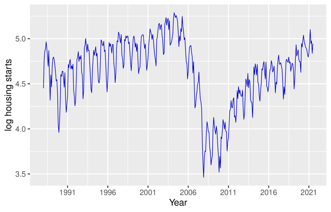
(a) Logarithm of housing starts.

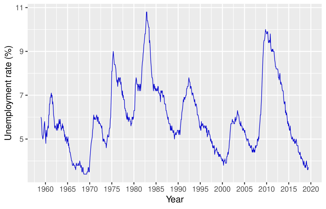
(b) Unemployment rates, seasonally adjusted.

Figure 1: Time plots of U.S. monthly housing starts and unemployment series

5.1 Housing starts in the U.S.

In this application, we are interested in modeling the logarithm of U.S. monthly housing starts. As depicted in Figure 1(a), the series exhibits an apparent seasonal pattern along with a drastic level change around the subprime financial crisis of 2008. For covariates, we collect the monthly new private housing units authorized by building permits for each state (for instance, data for Illinois are retrieved from https://fred.stlouisfed.org/series/ILBP1FH) and the 30-year fixed rate mortgage averages from the Economic Data of St. Louis Federal Reserve (Freddie Mac, 30-Year Fixed Rate Mortgage Average in the United States [MORTGAGE30US], retrieved from FRED, Federal Reserve Bank of St. Louis; https://fred.stlouisfed.org/series/MORTGAGE30US, October 27, 2022). After removing series with missing values, we have 49 housing permits series $\{x_{t,j},j=1,2,\ldots,49\}$ and the mortgage rate series $r_{t}$ from January 1988 through August 2022. We also remove the seasonality and unit root by taking $\tilde{x}_{t,j}=(1-B^{12})(1-B)\log x_{t,j}$, $j=1,2,\ldots,49$, and $\tilde{r}_{t}=r_{t}-r_{t-1}$. Consequently, we have 403 observations for each series.

Then we employ the following predictive model

$$h_{t}=\sum_{l=1}^{18}\alpha_{l}h_{t-l}+\sum_{j=1}^{49}\sum_{k=1}^{18}\beta_{k}^{(j)}\tilde{x}_{t-k,j}+\sum_{k=1}^{18}\beta_{k}^{(50)}\tilde{r}_{t-k}+\epsilon_{t},$$ (48)

where $h_{t}$ denotes the logarithm of U.S. housing starts at month $t$. Note that there are 918 potential predictors. We also consider the model with a drift,

$$h_{t}=\beta_{0}+\sum_{l=1}^{18}\alpha_{l}h_{t-l}+\sum_{j=1}^{49}\sum_{k=1}^{18}\beta_{k}^{(j)}\tilde{x}_{t-k,j}+\sum_{k=1}^{18}\beta_{k}^{(50)}\tilde{r}_{t-k}+\epsilon_{t}.$$ (49)

In implementing FHTD, we estimate (49) via the following procedure. Subtract first from each variable (including the dependent variable) its own sample average, and then apply FHTD to the transformed data. Finally, (49) is estimated by OLS with the selected variables and an intercept.

We perform rolling-window one-step-ahead prediction using FHTD as well as the other methods described in Section 4. We reserve the last 18 years of data as the test set, resulting in $W=216$ windows. Each window contains 169 observations as training data. Figure 2 plots some selected windows. As shown in the figure, the methods are challenged to forecast the sharp dip around 2008 and the following recovery. Since the true model is unknown, the performance of the methods under consideration is measured by the root mean squared prediction error (RMSE) and the median absolute prediction error (MAE), where $\mathrm{RMSE}=\{W^{-1}\sum_{w=1}^{W}(h_{T-w+1}-\hat{h}_{T-w+1})^{2}\}^{1/2}$ and MAE is the median of $\{|h_{T-w+1}-\hat{h}_{T-w+1}|:w=1,2\ldots,W\}$, in which $T$ is the time index for the last data point and $\hat{h}_{T-w+1}$ is the predicted value of $h_{T-w+1}$. In implementing FHTD and AR-OGA-3, we use HDIC in (44), $\hat{H}_{n}$ in (45), and choose $c$ and $d$ therein over a grid of values between 0.1 and 0.7 via a hold-out validation set consisting of the last $20\%$ of the training data in each window. The BIC is used to select the penalty parameters for LASSO-type methods.

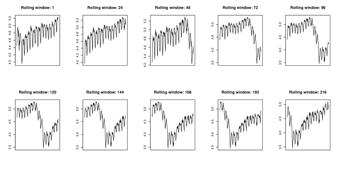
Figure 2: Time plots of logarithim of monthly U.S. Housting Starts, $h_{t}$, of selected windows

The prediction results are recorded in Table 3. Note that LASSO-type methods are highly sensitive to the specification of the intercept. They performed poorly when the intercept is omitted. In view of Figure 2, fitting the drift term to the upward trend in the first few windows may help alleviate the unit-root property in the data in finite sample, and without the drift, LASSO-type methods are unable to adapt to the unit-root behavior in the data. On the contrary, FHTD remains stable whether or not an intercept is included, and its prediction errors are substantially lower than the other methods.

Table 3: Out-of-sample RMSEs and MAEs of competing methods applied to (48) and (49)

	FHTD	OGA-3	AR-OGA-3	LASSO	ALasso	AR-ALasso
Model $\eqref{HS1}$
RMSE($\times 10$)	1.08	1.34	1.32	2.14	2.13	1.43
MAE($\times 10$)	0.72	0.82	0.82	1.21	1.17	0.97
Model $\eqref{HS2}$
RMSE($\times 10$)	1.11	1.31	1.29	1.24	1.21	1.14
MAE($\times 10$)	0.71	0.82	0.91	0.86	0.88	0.81

5.2 U.S. unemployment rate

Next, we consider the U.S. monthly unemployment rate $\{u_{t}\}$, shown in Figure 1(b). In some empirical studies, the unemployment rate is considered difference-stationary. Nevertheless, Bierens (2001) has found some evidence that the fluctuations in $\{u_{t}\}$ may be due to complex unit roots. Montgomery et al. (1998) have also noted the possibility of complex unit roots. Regardless of such complications, we can directly apply FHTD and the other methods discussed in the previous section to select a model for $\{u_{t}\}$ and to predict its future values. The data used are from the FRED-MD dataset (available on https://research.stlouisfed.org/econ/mccracken/fred-databases/), which contains 128 U.S. monthly macroeconomic variables from January 1959 to July 2019.

We use data from January 1973 to June 2019 and again consider rolling-window one-step-ahead predictions. After discarding the series with missing values during the time span, there remain 124 macroeconomic time series that can be used to forecast $u_{t}$. Following McCracken and Ng (2016), we transform some series by taking logs, differencing, or both, so that all 124 series are considered stationary after the transformations. Denote these series by $\{x_{t,j}\},j=1,\ldots,124$. Then we apply FHTD to the following model,

$$u_{t}=\sum_{i=1}^{6}\alpha_{i}u_{t-i}+\sum_{j=1}^{124}\sum_{l=1}^{6}\beta_{l}^{(j)}x_{t-l,j}+\epsilon_{t},$$ (50)

which contains 750 candidate predictors. The last two years of data are reserved as test samples, resulting in a window size of 310 observations.

The results are reported in Table 4. In both performance measures, FHTD outperforms OGA-3, AR-OGA-3, AR-ALasso, and LASSO. Its RMSE improves by $6\%$, $7\%$, $12\%$, and $14\%$ over OGA-3, LASSO, AR-OGA-3, and AR-ALasso, respectively. The results are similar when comparing the MAEs. Note that for LASSO, ALasso, and AR-ALasso, we only report their performance when an intercept is included, since, as observed in the previous application, these methods performed poorly when the intercept is omitted. In this particular application, without the intercept the RMSEs and MAEs of LASSO and ALasso can be more than 14 times as large as their counterparts for the AR-AIC. These results, combined with those in Table 3, show that FHTD is applicable to general unit-root time series, stable across specifications, and makes best use of the available predictors. Finally, we remark that the performance of ALasso (with intercept) is also quite competitive, implying that both are the most recommendable approaches to forecast $\{u_{t}\}$.

Table 4: Out-of-sample RMSEs and MAEs of competing methods applied to (50) for U.S. monthly unemployment rate series.

	FHTD	OGA-3	AR-OGA-3	LASSO	ALasso	AR-ALasso
RMSE($\times 10$)	1.34	1.42	1.50	1.44	1.38	1.52
MAE($\times 10$)	0.88	0.91	0.95	0.96	0.88	1.00

6 Concluding remarks

This paper proposed the FHTD algorithm for variable selection in high-dimensional nonstationary ARX models with heteroscedastic covariates and errors. Under strong sparsity conditions, we established its selection consistency, valid even when the lagged dependent variables are highly correlated and sample covariance matrices lack deterministic limits. Finally, we point out some potential research directions. First, shifting from (SS) and (SS_X) to weak sparsity assumptions (where coefficients are mostly non-zero but only a few are significant) may prioritize optimal forecasting over variable selection consistency. Addressing this issue remains challenging, particularly in the presence of complex unit roots. Another intriguing avenue is the model selection for cointegrated data, common in economics and environmental studies, within the realm of high-dimensional data analysis.

Appendix A Key technical tools

As noted earlier, the analysis of FHTD relies on a number of key theoretical tools, which are of independent interests. In particular, Theorems A.1–A.3 presented in this section not only are indispensable to our analysis, but may also be of use in future research related to unit-root ARX models with high-dimensional inputs. Their proofs can be found in Section S2 of the supplementary material.

Let

$$\begin{split}&\mathbb{B}_{n}(t_{1},t_{2},\ldots,t_{2l+2})\\ &=\frac{1}{\sqrt{n}}\left(\sum_{k=1}^{\lfloor nt_{1}\rfloor}\delta_{k},\sum_{k=1}^{\lfloor nt_{2}\rfloor}(-1)^{k}\delta_{k},\sum_{k=1}^{\lfloor nt_{3}\rfloor}\sqrt{2}\sin(k\vartheta_{1})\delta_{k},\sum_{k=1}^{\lfloor nt_{4}\rfloor}\sqrt{2}\cos(k\vartheta_{1})\delta_{k},\ldots,\sum_{k=1}^{\lfloor nt_{2l+2}\rfloor}\sqrt{2}\cos(k\vartheta_{l})\delta_{k}\right).\end{split}$$ (51)

Note that $\mathbb{B}_{n}$ is a random element in $D^{2l+2}$, where $D$ is the Skorohod space $D=D[0,1]$ (Billingsley, 1999). Our first theoretical apparatus is a novel FCLT for the multivariate linear processes (LABEL:ingapr10) under a set of mild conditions.

Theorem A.1.

Assume that (A1)–(A4) hold with $\eta$ in (11), (16), and (17) replaced by some $\eta_{1}>1$. In addition, assume

$$\max_{1\leq j\leq p_{n}}r_{j}^{(n)}=o(n^{\kappa}),$$ (52)

where $\kappa=\min\{1/2,1-\eta_{1}^{-1}\}$. Then

$$\mathbf{V}^{-1/2}\mathbb{B}_{n}\Rightarrow\mathbb{W},$$ (53)

where $\Rightarrow$ denotes convergence in law, $\mathbb{W}$ is a $(2l+2)$-dimensional standard Brownian motion, and $\mathbf{V}=\mathrm{diag}(v_{1}^{2},v_{2}^{2},\ldots,v_{2l+2}^{2})$ is a $(2l+2)$-dimensional diagonal matrix with

$$v_{1}^{2}=\sum_{h=-\infty}^{\infty}\gamma_{h},\,\,v_{2}^{2}=\sum_{h=-\infty}^{\infty}(-1)^{h}\gamma_{h},\,\,v_{2k+1}^{2}=v_{2k+2}^{2}=\sum_{h=-\infty}^{\infty}\cos(h\vartheta_{k})\gamma_{h},$$

$k=1,2,\ldots,l$.

Note that $v_{i}^{2}>0,i=1,\ldots,2l+2$, are ensured by (A3). If (2) reduces to an AR($p$) model with a fixed $p$ and a GARCH error $\epsilon_{t}$, then $v_{m}^{2}=\sigma^{2}$ for all $m$, and the weak limit in Theorem A.1 coincides with Theorem 3.3 of Ling and Li (1998). Furthermore, when the error $\epsilon_{t}$ reduces to an m.d.s. with constant conditional variance, Theorem A.1 reduces to Theorem 2.2 of Chan and Wei (1988). Here, due to the presence of $v_{t,n}=\sum_{j=1}^{p_{n}}\sum_{l=1}^{r_{j}^{(n)}}\beta_{l}^{(j)}x_{t-l,j}$ in $\delta_{t}$, the FCLT is quite different from the classical ones, where the linear processes are driven by $\{\epsilon_{t}\}$ only.

Theorem A.2.

Let

$$X_{i}=\sum_{l=-\infty}^{i}a_{i,l}\tilde{x}_{l},\;\;Y_{j}=\sum_{k=-\infty}^{j}b_{j,k}\tilde{y}_{k},$$

where $\sum_{l=-\infty}^{i}a^{2}_{i,l}<\infty$ and $\sum_{k=-\infty}^{j}b^{2}_{j,k}<\infty$, for all $1\leq i,j\leq n$, and $\{(\tilde{x}_{t},\tilde{y}_{t}),\mathcal{F}_{t}\}$ is an m.d.s. Suppose also

$$\tilde{x}_{t}\tilde{y}_{t}-\operatorname{\mathbb{E}}(\tilde{x}_{t}\tilde{y}_{t})=\sum_{j=0}^{\infty}\bm{\theta}_{j}^{\top}\tilde{\mathbf{z}}_{t-j},$$ (54)

where $\{\tilde{\mathbf{z}}_{t},\mathcal{F}_{t}\}$ is a multivariate m.d.s. and $\sum_{j=0}^{\infty}\|\bm{\theta}_{j}\|\leq C$, and

$$\sup_{t}\{\operatorname{\mathbb{E}}|\tilde{x}_{t}|^{p}+\operatorname{\mathbb{E}}|\tilde{y}_{t}|^{q}+\operatorname{\mathbb{E}}\|\tilde{\mathbf{z}}_{t}\|^{2r}\}\leq C,$$ (55)

where $1/p+1/q=1/(2r)$ for some $r\geq 1$. Define $Q_{n}=\sum_{i,j=1}^{n}q_{i,j}X_{i}Y_{j}$, where $q_{i,j}$ are real numbers. Then,

$$\operatorname{\mathbb{E}}|Q_{n}-\operatorname{\mathbb{E}}Q_{n}|^{2r}\leq C_{r}\left\{\operatorname{\mathbb{E}}\left(\sum_{i,j=1}^{n}q_{i,j}X_{i}^{*}Y_{j}^{*}\right)^{2}\right\}^{r},$$

where $C_{r}$ is a positive constant depending only on $r$,

$$X_{i}^{*}=\sum_{l=-\infty}^{i}a_{i,l}x_{l}^{*},\quad Y_{j}^{*}=\sum_{k=-\infty}^{j}b_{j,k}y_{k}^{*},$$

and $\{x_{t}^{*}\}$ and $\{y_{t}^{*}\}$ are independent processes that are identically distributed with $\{\tilde{x}_{t}\}$ and $\{\tilde{y}_{t}\}$, respectively.

Theorem A.2 provides a novel moment bound for quadratic forms of linear processes driven by conditional heteroscedastic m.d.s., and it resembles the First Moment Bound theorem of Findley and Wei (1993), with some essential improvements. First, their theorem assumes that the $\tilde{x}_{t}$ and $\tilde{y}_{t}$ in (54) obey $\operatorname{\mathbb{E}}(\tilde{x}_{t}\tilde{y}_{t}|\mathcal{F}_{t-1})=\operatorname{\mathbb{E}}(\tilde{x}_{t}\tilde{y}_{t})$ a.s.; hence the conditional heteroscedasticity is precluded. On the other hand, as discussed in Section S1 in the supplementary material, (54) permits many conditionally heteroscedastic processes. Finally, (55) allows $\tilde{x}_{t}$ and $\tilde{y}_{t}$ to be integrable up to different orders, which helps deal with quadratic forms involving $\{\epsilon_{t}\}$ and $\{x_{t,j}\}$ in (2) since they may exhibit different tail behaviors. Theorem A.1 and Theorem A.2 are crucial for the following uniform lower bound for the minimum eigenvalues of the sample covariance matrices.

Theorem A.3.

Assume (A1)–(A5) and (21). Then, for

$$K_{n}=o(n^{1/2}/{p_{n}^{*}}^{\bar{\theta}}),$$ (56)

where $\bar{\theta}$ is defined in (SS_X),

$$\max_{\sharp(J)\leq K_{n}}\lambda_{\min}^{-1}\left(n^{-1}\sum_{t=\bar{r}_{n}+1}^{n}\mathbf{s}_{t}(J)\mathbf{s}_{t}^{\top}(J)\right)=O_{p}(1),$$ (57)

where $\mathbf{s}_{t}(J)$ is defined in Section S2 of the supplementary material. Moreover,

$$\max_{\sharp(J)\leq K_{n}}\lambda_{\min}^{-1}\left(n^{-1}\sum_{t=\bar{r}_{n}+1}^{n}\mathbf{w}_{t}(J)\mathbf{w}_{t}^{\top}(J)\right)=O_{p}(1).$$ (58)

Theorem A.3 highlights one of the most intriguing subtleties of our analysis. Since our predictors contain highly correlated lagged dependent variables, it is not known a priori whether they lead to asymptotically ill-conditioned (or even singular) sample covariance matrices. This issue is resolved through the FCLT (Theorem A.1), and Theorem A.3 thus suggests that model selection criteria based on least squares can differentiate between candidate predictors, albeit containing $q_{n}$ highly correlated AR variables. Equations (58) and (57), respectively, are also aligned with (3.10) of Lai and Wei (1982) and (3.5.1) of Chan and Wei (1988), in which model (2) is simplified to a finite-order nonstationary AR model with a conditionally homogeneous error.

Supplement for “Model Selection for Unit-root Time Series with Many Predictors” The supplementary material contains the theoretical proofs of Theorem 3.1–3.3, Theorems A.1–A.3, and further technical discussions, including some remarks on Assumptions (A1)–(A6), (SS_X), and (SS) as well as further information regarding Example 3.1 and 3.1. Additional simulation results are also presented.

This supplemental material contains five sections. Section S1 provides comments on Assumptions (A1)–(A6) and discusses the sparsity conditions (SS_X) and (SS). Section S2 presents proofs for the main results, Theorems 3.1–3.3 of the paper, as well as the proofs of Theorem A.1–A.3. Further details related to Section S2 can be found in Section S3. Section S4 contains specific information regarding Examples 3.1 and 3.2. Finally, Section S5 offers additional simulation results.

Appendix S1 Comments on Assumptions (A1)–(A6), (SS_X), and (SS)

In this section, we provide some comments on Assumptions (A1)–(A6). Assumption (A1) is fulfilled by many conditionally heteroscedastic processes. For example, consider a stationary GJR-GARCH$(p_{0}^{\prime},q_{0}^{\prime})$ model (Glosten, Jagannathan and Runkle, 1993),

$$\begin{split}\epsilon_{t}=\nu_{t}z_{t},\,\,\nu_{t}^{2}=\operatorname{\mathbb{E}}(\epsilon_{t}^{2}|{\cal F}_{t-1})=\varphi_{0,0}+\sum_{i=1}^{p^{\prime}_{0}}\varphi_{0,i}\epsilon_{t-i}^{2}+\sum_{j=1}^{q^{\prime}_{0}}\psi_{0,j}\nu_{t-j}^{2}+\sum_{k=1}^{p_{0}^{\prime}}\zeta_{0,k}\epsilon_{t-k}^{2}\mathbb{I}_{\{\epsilon_{t-k}<0\}},\end{split}$$ (S1.1)

where $z_{t}$ are independent and identically distributed (i.i.d.) symmetric random variables with zero mean, unit variance, and finite 2$\eta$-th moment, $\eta\geq 2$, $\mathcal{F}_{t}=\sigma(z_{s},s\leq t)$, $p^{\prime}_{0}$ and $q^{\prime}_{0}$ are positive integers, $\varphi_{0,0}>0$, and $\varphi_{0,i}$, $\psi_{0,j}$, and $\zeta_{0,k}$ are non-negative constants that guarantee $\operatorname{\mathbb{E}}|\epsilon_{1}|^{2\eta}<\infty$. Following Huang et al. (2022), it can be shown that (A1) is fulfilled by (S1.1) with $l_{0}=2$, $\mathbf{e}_{t}=(w_{1,t},w_{2,t})^{\top}$, and $\bm{\theta}_{s}=(\tilde{b}_{s},\tilde{c}_{s})^{\top}$, where $w_{1,t}=\epsilon_{t}^{2}-\nu_{t}^{2}$, $w_{2,t}=\epsilon_{t}^{2}I_{\{\epsilon_{t}<0\}}-\frac{1}{2}\epsilon_{t}^{2}$, and $\tilde{b}_{j}$ and $\tilde{c}_{j}$, respectively, satisfy

$$\sum_{j=0}^{\infty}\tilde{b}_{j}z^{j}=\frac{1-\sum_{j=1}^{q_{0}^{{}^{\prime}}}\psi_{0,j}z^{j}}{1-\sum_{i=1}^{\max\{p_{0}^{\prime},q_{0}^{\prime}\}}(\varphi_{0,i}+\psi_{0,i}+\frac{\zeta_{0,i}}{2})z^{j}}$$

and

$$\sum_{j=0}^{\infty}\tilde{c}_{j}z^{j}=\frac{\sum_{j=1}^{p_{0}^{{}^{\prime}}}\zeta_{0,j}z^{j}}{1-\sum_{i=1}^{\max\{p_{0}^{\prime},q_{0}^{\prime}\}}(\varphi_{0,i}+\psi_{0,i}+\frac{\zeta_{0,i}}{2})z^{j}},$$

in which $\psi_{0,j}=0$ if $j>q_{0}^{\prime}$, $\varphi_{0,i}=\zeta_{0,i}=0$ if $i>p_{0}^{\prime}$, and $\sum_{i=1}^{p^{\prime}_{0}}\varphi_{0,i}+\sum_{j=1}^{q^{\prime}_{0}}\psi_{0,j}+\sum_{k=1}^{p^{\prime}_{0}}\frac{\zeta_{0,k}}{2}<1$. When $\zeta_{0,k}=0$ for all $k$, (S1.1) reduces to the well-known stationary GARCH ($p_{0}^{\prime},q_{0}^{\prime}$) process; the same argument ensures that (A1) holds with $l_{0}=1$, $e_{t}=w_{1,t}$, and $\theta_{s}=\tilde{b}_{s}$.

Assumption (A2) requires that $\{x_{t,s}\}$ is an MA($\infty$) process driven by the conditionally heteroscedastic innovations $\{\pi_{t,s}\}$. This type of assumption is broadly adopted in time series analysis. In fact, (A2) allows $(\epsilon_{t},\pi_{t,1}\ldots,\pi_{t,p_{n}})^{\top}$ to be a multivariate GARCH process. By the same argument used in the previous paragraph, it can be shown that the diagonal VEC model of Bollerslev, Engle and Wooldridge (1988) is a special case of (14). Furthermore, in the notable special case where $\{\pi_{t,s}\}$ is a sequence of independent and identically distributed random variables with $\operatorname{\mathbb{E}}(\pi_{t,s})=0$ and $\operatorname{\mathbb{E}}(\pi_{t,s_{1}}\pi_{t,s_{2}})=\sigma_{s_{1},s_{2}}$, (14) remains valid, with $e_{t,s_{1},s_{2}}=\pi_{t,s_{1}}\pi_{t,s_{2}}-\sigma_{s_{1},s_{2}}$, $\theta_{0,s_{1},s_{2}}=1$, and $\theta_{j,s_{1},s_{2}}=0$ for $j>0$. Moment conditions (16) and (17) are more stringent than (11). These stronger moment assumptions ensure a reliable screening performance of FSR when the number of exogenous covariates is larger than the sample size, as allowed by Assumption (A5).

Assumption (A3) is used to derive Theorem A.1, leading to a uniform lower bound for the minimum eigenvalues of the sample covariance matrices of dimensions less than or equal to $q_{n}+K_{n}$; see the proof for Theorem A.3. Assumption (A4), referred to as the weak sparsity condition, is commonly used in the literature on high-dimensional data analysis. It follows from (12), (13), and (A4) that

$$\sup_{n\geq 1}\sum_{h=-\infty}^{\infty}|\gamma_{h,n}|\leq C,$$ (S1.2)

which, together with (18), leads to

$$\sum_{h=-\infty}^{\infty}|\gamma_{h}|\leq C.$$ (S1.3)

When the moment conditions are controlled, (A5) is more flexible than the assumptions on model dimensions in Medeiros and Mendes (2016), where $\{y_{t}\}$ is assumed to be stationary, corresponding to the case of $a=b=d_{1}=\cdots=d_{l}=0$. To see this, note that (A1) and (A2) imply (19) and (20) respectively. Moreover, (A1), together with (A2), yields

$$\sup_{t}\operatorname{\mathbb{E}}|y_{t}|^{2\eta}<C,$$ (S1.4)

provided $a=b=d_{1}=\cdots=d_{l}=0$. By (19), (20), (S1.4), and Hölder’s inequality,

$$\sup_{t}\operatorname{\mathbb{E}}|y_{t-i}\epsilon_{t}|^{\eta}<C\,\,\mbox{and}\,\,\sup_{t}\operatorname{\mathbb{E}}|x_{t-l,j}\epsilon_{t}|^{2\eta q_{0}/(q_{0}+1)}<C,$$

for all $1\leq i\leq q_{n}$, $1\leq l\leq r_{j}^{(n)}$, and $1\leq j\leq p_{n}$. Therefore, the $m$ in Assumption DGP(4) of Medeiros and Mendes (2016) obeys

$$m=\min\{\eta,2\eta q_{0}/(q_{0}+1)\}=\eta.$$ (S1.5)

Equation (S1.5) and the discussion after Assumption (REG) of Medeiros and Mendes (2016) lead to a restriction on the number of candidate variables such that

$$q_{n}+p_{n}^{*}=o(n^{\alpha\eta(\eta-2)/(2\eta+4b)}),$$ (S1.6)

where $0<\alpha<1$ and $b>0$ are positive numbers defined therein. Equation (S1.6) requires $p_{n}^{*}$ to be much smaller than $n$ unless $\eta>4$. In contrast, (A5) allows $p_{n}^{*}>n$ even if $\eta=2$.

We also make a few comments on (A6). For $D\subset\{1,\ldots,p_{n}\}$, let

$$\begin{split}&\bm{\pi}_{t}(D)=(\pi_{t,s}:s\in D)^{\top},\,\,\bm{\mu}_{t}(D)=(\epsilon_{t},\bm{\pi}^{\top}_{t}(D))^{\top},\\ &\mathbf{\bm{\Sigma}}_{n}(D)=\operatorname{\mathbb{E}}(\bm{\mu}_{t}(D)\bm{\mu}^{\top}_{t}(D)).\end{split}$$ (S1.7)

Then, it can be shown that (21) holds if $\{x_{t,j}\}$ admits an infinite-order AR representation with absolutely summable coefficients and

$$\max_{\sharp(D)\leq K_{n}+\underline{s}_{0}}\lambda_{\min}^{-1}(\mathbf{\bm{\Sigma}}_{n}(D))\leq C,$$ (S1.8)

where $\underline{s}_{0}$ is defined in (SS_A). When the AR components are deleted from model (2), (22) reduces to (3.2) of Ing and Lai (2011), which is closely related to the “exact recovery condition” introduced by Tropp (2004) in the analysis of the orthogonal matching pursuit and plays a role similar to the “restricted eigenvalue assumption” introduced by Bickel, Ritov and Tsybakov (2009) in the study of LASSO. Condition (22) is a natural generalization of (3.2) of Ing and Lai (2011) when the (asymptotically) stationary AR component, $\mathbf{z}_{t}(q_{n}-d)=(z_{t-1},\ldots,z_{t-q_{n}+d})^{\top}$, is taken into account.

We now present an example that illustrates the validity of (22) even when model (2) includes highly correlated lagged dependent variables and highly correlated exogenous variables. Assume in model (2) that $r_{j}^{(n)}=1$ for all $1\leq j\leq p_{n}$ and $\{(x_{t-1,1},\ldots,x_{t-1,p_{n}},\epsilon_{t})^{\top}\}$ is a sequence of white noise vectors obeying $\operatorname{\mathbb{E}}(\epsilon_{t}^{2})=\operatorname{\mathbb{E}}(x_{t,j}^{2})=1$ for all $1\leq j\leq p_{n}$ and $0\leq\operatorname{\mathbb{E}}(x_{t,i}x_{t,j})=\operatorname{\mathbb{E}}(x_{t,l}\epsilon_{t})=\lambda<1$ for all $1\leq i\neq j\leq p_{n}$ and $1\leq l\leq p_{n}$. In this model specification, not only are $y_{t-j},1\leq j\leq q_{n}$, highly correlated, but also $x_{t-1,j},1\leq j\leq p_{n}$, especially when $\lambda$ is close to 1. Define $\mathbf{G}(q_{n}-d)=[\mathbf{G}_{ij}]_{1\leq i,j\leq q_{n}-d}=\operatorname{\mathbb{E}}^{-1}(\mathbf{z}_{t,\infty}(q_{n}-d)\mathbf{z}_{t,\infty}^{\top}(q_{n}-d))$ and $c_{J}^{2}=\lambda^{2}\sharp(J)/(1-\lambda+\sharp(J)\lambda)$. Since $0<c_{J}^{2}<\lambda$ and $0<\mathbf{G}_{11}\leq 1$, it holds that

$$\max_{\sharp(J)\leq K_{n},(i,1)\notin J}\sum_{(i^{*},1)\in J}|a_{i^{*},1}(i,1)|\leq\max_{\sharp(J)\leq K_{n}}\frac{(1-\lambda\mathbf{G}_{11})\lambda\sharp(J)}{(1-c_{J}^{2}\mathbf{G}_{11})(1-\lambda+\sharp(J)\lambda)}\leq 1.$$ (S1.9)

Moreover, one has

$$\begin{split}\sum_{s=1}^{q_{n}-d}\max_{\sharp(J)\leq K_{n},(i,1)\notin J}|a_{s,J}(i,1)|\leq\sum_{s=1}^{q_{n}-d}\max_{\sharp(J)\leq K_{n}}\frac{\lambda-c_{J}^{2}}{1-c_{J}^{2}\mathbf{G}_{11}}|\mathbf{G}_{s1}|\leq\sum_{s=1}^{q_{n}-d}|\mathbf{G}_{s1}|.\end{split}$$ (S1.10)

Define $a^{2}=1+\lambda(\sum_{j=1}^{p_{n}}\beta_{1}^{(j)})^{2}+(1-\lambda)\sum_{j=1}^{p_{n}}(\beta_{1}^{(j)})^{2}$, $b=\lambda\sum_{j=1}^{p_{n}}\beta_{1}^{(j)}$, and $h^{2}=(a^{2}+(a^{4}-4b^{2})^{1/2})/2$, noting that $|b|<a^{2}/2$ and

$$h^{2}>\max\{1,\lambda(\sum_{j=1}^{p_{n}}\beta_{1}^{(j)})^{2}+(1-\lambda)\sum_{j=1}^{p_{n}}(\beta_{1}^{(j)})^{2}\}.$$ (S1.11)

Then, it can be shown that $\{z_{t,\infty}\}$ admits an infinite-order AR representation,

$$z_{t,\infty}+\sum_{j=1}^{\infty}\phi_{j}z_{t-j,\infty}=\eta_{t},$$ (S1.12)

where $1+\sum_{j=1}^{\infty}\phi_{j}z^{j}\neq 0$, for $|z|\leq 1$, $\sum_{j=0}^{\infty}|\phi_{j}|\leq C$, and $\{\eta_{t}\}$ is a white noise sequence with variance $h^{2}$. By using a modified Cholesky decomposition (e.g., Ing, Chiou and Guo (2016)), (S1.11), (S1.12), and Baxter’s inequality (Baxter, 1962), one gets $\sum_{s=1}^{q_{n}-d}|\mathbf{G}_{s1}|\leq Ch^{-2}\sum_{j=0}^{\infty}|\phi_{j}|\leq C$, which, together with (S1.9) and (S1.10), leads to (22).

Finally, we provide a brief discussion of the strong sparsity conditions (SS_X) and (SS) in Sections 3.2 and 3.3. As mentioned earlier, a condition similar to (SS_X) has been utilized by Medeiros and Mendes (2016) to establish the selection consistency of the adaptive LASSO when $\{y_{t}\}$ is stationary. Specifically, they assume

$$\frac{\lambda s_{0}^{1/2}}{n^{1-\xi/2}\phi_{\min}}=o(\min_{\begin{subarray}{c}(j,l)\in{\cal J}_{n}\end{subarray}}|{\beta_{l}^{(j)}}|),$$ (S1.13)

where $0<\xi<1$ is some constant defined in their Assumption (WEIGHTS) and $2\phi_{\min}$ is a lower bound for the minimum eigenvalue of the covariance matrix of the random vector formed by all relevant predictors. Assuming that $\phi_{\min}$ is bounded away from 0 and choosing $\lambda$ to be the value suggested after Assumption (REG) of Medeiros and Mendes (2016), (S1.13) becomes

$$\frac{s_{0}^{1/2}p_{n}^{*^{1/m}}n^{\xi/m}}{n^{1/2}}=o(\min_{\begin{subarray}{c}(j,l)\in{\cal J}_{n}\end{subarray}}|{\beta_{l}^{(j)}}|).$$ (S1.14)

In view of (S1.5) and the definitions of $\bar{\theta}$ and $\xi$, we conclude that (S1.14) is more stringent than (23) in (SS_X). While the left-hand side of (33) in (SS) is larger than that of (23) by a factor about $(\log n)^{1/2}$, it is still smaller than that of (S1.14).

Appendix S2 Main proofs

In this section, we present the proofs of the main results in the paper, namely Theorems 3.1–3.3. The proofs, shown in Section S2.2, are proceeded by the proofs for Theorems A.1–A.3. Some further details regarding the proofs are collected in Section S2.3.

S2.1 Proofs of Theorems A.1–A.3 and discussions

Proof of Theorem A.1.

Let $a_{t}^{(m)}$, $t\geq 1$ and $1\leq m\leq 2l+2$, be defined by $a_{t}^{(1)}=1,a_{t}^{(2)}=(-1)^{t},a_{t}^{(3)}=\sqrt{2}\sin(t\vartheta_{1}),a_{t}^{(4)}=\sqrt{2}\cos(t\vartheta_{1}),\ldots,a_{t}^{(2l+1)}=\sqrt{2}\sin(t\vartheta_{l})$, and $a_{t}^{(2l+2)}=\sqrt{2}\cos(t\vartheta_{l})$. Note first that each element of $\mathbb{B}_{n}$ is of the form

$$\frac{1}{\sqrt{n}}\sum_{t=1}^{\lfloor nu\rfloor}a_{t}\delta_{t},$$ (S2.1)

where $u\in[0,1]$ and $\{a_{t}\}$ is one of $\{a_{t}^{(m)}\},1\leq m\leq 2l+1$. In Section S2.3, we show that (S2.1) has the following decomposition

$$\frac{1}{\sqrt{n}}\sum_{t=1}^{\lfloor nu\rfloor}a_{t}\delta_{t}=R_{n}(u)+\sum_{t=1}^{\lfloor nu\rfloor-1}\left(X_{t,n}+\frac{a_{t}}{\sqrt{n}}\epsilon_{t}\right)+\frac{a_{\lfloor nu\rfloor}}{\sqrt{n}}\epsilon_{\lfloor nu\rfloor},$$ (S2.2)

where

$$X_{t,n}=\frac{1}{\sqrt{n}}\sum_{j=1}^{p_{n}}\left[\sum_{s=t+1}^{n}a_{s}\left(\sum_{l=1}^{(s-t)\wedge r_{j}}\beta_{l}^{(j)}p_{s-l-t,j}\right)\right]\pi_{t,j},$$

and $R_{n}(u)$ is a remainder term whose explicit form is given in Section S2.3. By Assumption (A1),

$$\sup_{t}\mathbb{E}|\epsilon_{t}|^{2\eta_{1}}<C,$$ (S2.3)

yielding

$$\sup_{u\in[0,1]}\frac{|a_{\lfloor nu\rfloor}\epsilon_{\lfloor nu\rfloor}|}{\sqrt{n}}=o_{p}(1)$$ (S2.4)

and

$$\mathbb{E}\big{(}\frac{a^{2}_{\lfloor nu\rfloor}\epsilon^{2}_{\lfloor nu\rfloor}}{n}\big{)}=o(1),\,\,u\in[0,1].$$ (S2.5)

By Assumption (A2),

$$\sup_{t}\max_{1\leq j\leq p_{n}}\operatorname{\mathbb{E}}|\pi_{t,j}|^{2\eta_{1}}\leq C.$$ (S2.6)

Using (S2.6), after some algebraic manipulations, we show in Section S2.3 that

$$\sup_{u\in[0,1]}|R_{n}(u)|= o_{p}(1),$$ (S2.7)

$$\operatorname{\mathbb{E}}R_{n}^{2}(u)= o(1),\;u\in[0,1].$$ (S2.8)

By (S2.2), (S2.4), and (S2.7), (53) in the main paper holds if

$$\left(v_{1}^{-1}\sum_{t=1}^{\lfloor nu_{1}\rfloor-1}\left(X_{t,n}^{(1)}+\frac{a_{t}^{(1)}}{\sqrt{n}}\epsilon_{t}\right),\ldots,v_{2l+2}^{-1}\sum_{t=1}^{\lfloor nu_{2l+2}\rfloor-1}\left(X_{t,n}^{(2l+2)}+\frac{a_{t}^{(2l+2)}}{\sqrt{n}}\epsilon_{t}\right)\right)\Rightarrow\mathbb{W},$$ (S2.9)

where $X_{t,n}^{(m)}$ is $X_{t,n}$ with $a_{s}=a_{s}^{(m)}$, and $u_{j}\in[0,1]$ for $1\leq j\leq 2l+2$. Define

$$\xi_{t,n}^{(m)}=v_{m}^{-1}(X_{t,n}^{(m)}+\frac{a_{t}^{(m)}}{\sqrt{n}}\epsilon_{t}).$$

Note that $\{(\xi_{t,n}^{(1)},\ldots,\xi_{t,n}^{(2l+2)})^{\top},\mathcal{F}_{t}\}$ is an m.d.s. By Theorem 3.3 of Helland (1982), (S2.9) follows if

$$\sum_{t=1}^{\lfloor nu\rfloor}\operatorname{\mathbb{E}}({\xi_{t,n}^{(m)}}^{2}|\mathcal{F}_{t-1})\stackrel{{\scriptstyle p}}{{\rightarrow}}u,\;1\leq m\leq 2l+2,$$ (S2.10)

$$\sum_{t=1}^{\lfloor nu\rfloor}\operatorname{\mathbb{E}}({|\xi_{t,n}^{(m)}}|^{2+c}|\mathcal{F}_{t-1})\stackrel{{\scriptstyle p}}{{\rightarrow}}0,\;1\leq m\leq 2l+2,$$ (S2.11)

for some $c>0$, and

$$\sum_{t=1}^{\lfloor nu\rfloor}\operatorname{\mathbb{E}}(\xi_{t,n}^{(k)}\xi_{t,n}^{(m)}|\mathcal{F}_{t-1})\stackrel{{\scriptstyle p}}{{\rightarrow}}0,\;1\leq k\neq m\leq 2l+2.$$ (S2.12)

In the following, we only prove (S2.10) because (S2.12) can be proved similarly and (S2.11) follows directly from (S2.86) in Section S2.3. Let $\zeta_{t,n}^{(m)}=v_{m}\xi_{t,n}^{(m)}$. Then,

$$\begin{split}v_{m}^{2}\sum_{t=1}^{\lfloor nu\rfloor}\operatorname{\mathbb{E}}({\xi_{t,n}^{(m)}}^{2}|\mathcal{F}_{t-1})=&\sum_{t=1}^{\lfloor nu\rfloor}\operatorname{\mathbb{E}}({\zeta_{t,n}^{(m)}}^{2})-\sum_{t=1}^{\lfloor nu\rfloor}\big{\{}{\zeta_{t,n}^{(m)}}^{2}-\operatorname{\mathbb{E}}({\zeta_{t,n}^{(m)}}^{2}|\mathcal{F}_{t-1})\big{\}}\\ &+\sum_{t=1}^{\lfloor nu\rfloor}\big{\{}{\zeta_{t,n}^{(m)}}^{2}-\operatorname{\mathbb{E}}({\zeta_{t,n}^{(m)}}^{2})\big{\}}.\end{split}$$ (S2.13)

We show in Section S2.3 that

$$\operatorname{\mathbb{E}}\big{\{}\sum_{t=1}^{\lfloor nu\rfloor}\zeta_{t,n}^{(m)}\big{\}}^{2}\leq C,$$ (S2.14)

which, together with (S2.2), (S2.5), (S2.8), Assumption (A3), (S1.2), and (S1.3), gives, for $1\leq m\leq 2l+2$,

$$\lim_{n\rightarrow\infty}\sum_{t=1}^{\lfloor nu\rfloor}\operatorname{\mathbb{E}}({\zeta_{t,n}^{(m)}}^{2})=\lim_{n\rightarrow\infty}\operatorname{\mathbb{E}}\left(\frac{1}{\sqrt{n}}\sum_{t=1}^{\lfloor nu\rfloor}a_{t}^{(m)}\delta_{t}\right)^{2}=uv_{m}^{2}.$$ (S2.15)

Moreover, by making use of (S2.3), (S2.6), and Assumptions (A1) and (A2), we prove in Section S2.3 that

$$\big{|}\sum_{t=1}^{\lfloor nu\rfloor}\big{\{}{\zeta_{t,n}^{(m)}}^{2}-\operatorname{\mathbb{E}}({\zeta_{t,n}^{(m)}}^{2}|\mathcal{F}_{t-1})\big{\}}\big{|}+\big{|}\sum_{t=1}^{\lfloor nu\rfloor}\big{\{}{\zeta_{t,n}^{(m)}}^{2}-\operatorname{\mathbb{E}}({\zeta_{t,n}^{(m)}}^{2})\big{\}}\big{|}=o_{p}(1).$$ (S2.16)

Combining (S2.16) with (S2.15) and (S2.13), we have (S2.10). Thus, the proof is complete. ∎

Proof of Theorem A.2.

In the following, we denote by $C_{r}$ any generic absolute constant depending only on $r$ whose value may vary at different places. By some straightforward algebra, it is not difficult to see

$$\operatorname{\mathbb{E}}|Q_{n}-\operatorname{\mathbb{E}}Q_{n}|^{2r}=\operatorname{\mathbb{E}}\left|\sum_{l=-\infty}^{n}\sum_{k=-\infty}^{n}c_{k,l}\tilde{x}_{l}\tilde{y}_{k}-\operatorname{\mathbb{E}}Q_{n}\right|^{2r},$$

where $c_{k,l}=\sum_{i=l\vee 1}^{n}\sum_{j=k\vee 1}^{n}q_{i,j}a_{i,l}b_{j,k}$. Then observe that

$$\operatorname{\mathbb{E}}\left|\sum_{l=-\infty}^{n}\sum_{k=-\infty}^{n}c_{k,l}\tilde{x}_{l}\tilde{y}_{k}-\operatorname{\mathbb{E}}Q_{n}\right|^{2r}\leq C_{r}\left\{\operatorname{\mathbb{E}}\left|\sum_{l=-\infty}^{n}c_{l,l}(\tilde{x}_{l}\tilde{y}_{l}-\operatorname{\mathbb{E}}(\tilde{x}_{l}\tilde{y}_{l}))\right|^{2r}\right.$$

$$+\operatorname{\mathbb{E}}\left|\sum_{k=-\infty}^{n}\left(\sum_{l=-\infty}^{k-1}c_{k,l}\tilde{x}_{l}\right)\tilde{y}_{k}\right|^{2r}$$

$$+\left.\operatorname{\mathbb{E}}\left|\sum_{l=-\infty}^{n}\left(\sum_{k=-\infty}^{l-1}c_{k,l}\tilde{y}_{k}\right)\tilde{x}_{l}\right|^{2r}\right\}$$

$$:= C_{r}\{{\rm(I)+(II)+(III)}\}.$$

By Burkholder’s inequality, Minkowski’s inequality, Cauchy-Schwart inequality, and the fact that $\sup_{t}\operatorname{\mathbb{E}}\|\tilde{\mathbf{z}}_{t}\|^{2r}\leq C$, we have

$${\rm(I)}=\operatorname{\mathbb{E}}\left|\sum_{j=-\infty}^{n}\left(\sum_{l=j}^{n}c_{l,l}\bm{\theta}_{l-j}^{\top}\right)\tilde{\mathbf{z}}_{j}\right|^{2r}\leq C_{r}\left\{\sum_{j=-\infty}^{n}\left\|\left(\sum_{l=j}^{n}c_{l,l}\bm{\theta}_{l-j}^{\top}\right)\tilde{\mathbf{z}}_{j}\right\|^{2}_{2r}\right\}^{r}$$

$$\leq C_{r}\left\{\sum_{j=-\infty}^{n}\left\|\sum_{l=j}^{n}c_{l,l}\bm{\theta}_{l-j}\right\|^{2}\right\}^{r}.$$ (S2.17)

Note that

$$\sum_{j=-\infty}^{n}\left\|\sum_{l=j}^{n}c_{l,l}\bm{\theta}_{l-j}\right\|^{2}=\sum_{l=-\infty}^{n}\sum_{k=-\infty}^{n}c_{l,l}c_{k,k}\sum_{j=0}^{\infty}\bm{\theta}_{j}^{\top}\bm{\theta}_{j+|l-k|}\leq C\left(\sum_{j=0}^{\infty}\|\bm{\theta}_{j}\|\right)^{2}\left(\sum_{l=-\infty}^{n}c_{ll}^{2}\right).$$

This, combined with (S2.17) and $\sum_{j=0}^{\infty}\|\bm{\theta}_{j}\|\leq C$, yields

$${\rm(I)}\leq C_{r}\left\{\sum_{l=-\infty}^{n}c_{l,l}^{2}\right\}^{r}.$$ (S2.18)

Next, by Burkholder’s inequality, Minkowski’s inequality, Hölder’s inequality, and (55) in the main paper, we have

$${\rm(II)}\leq \left\{C_{r}\left\|\sum_{k=-\infty}^{n}\left(\sum_{l=-\infty}^{k-1}c_{k,l}\tilde{x}_{l}\right)^{2}\tilde{y}_{k}^{2}\right\|_{r}\right\}^{r}$$

$$\leq C_{r}\left\{\sum_{k=-\infty}^{n}\left\|\sum_{l=-\infty}^{k-1}c_{k,l}\tilde{x}_{l}\right\|_{p}^{2}\|\tilde{y}_{k}\|_{q}^{2}\right\}^{r}$$

$$\leq C_{r}\left\{\sum_{k=-\infty}^{n}\sum_{l=-\infty}^{k-1}c_{k,l}^{2}\right\}^{r}.$$ (S2.19)

By a similar argument, it can be shown that

$${\rm(III)}\leq C_{r}\left\{\sum_{l=-\infty}^{n}\sum_{k=-\infty}^{l-1}c_{k,l}^{2}\right\}^{r}.$$

This, in conjunction with (S2.18) and (S2.19), yields the desired conclusion. ∎

Theorems A.1 and A.2 can be used to bound from below the minimum eigenvalues of the sample covariance matrices of the candidate models; see Theorem A.3. To state this result, we need to introduce some notations.

Recall $\phi(B)$ in Section 3.1. Inspired by Chan and Wei (1988), we define

$$\begin{split}u_{t}(j)&=[(1-B)^{-j}\phi(B)]y_{t},\\ v_{t}(j)&=[(1+B)^{-j}\phi(B)]y_{t},\\ g_{t}(k,j)&=[(1-2\cos\vartheta_{k}B+B^{2})^{-j}\phi(B)]y_{t},\end{split}$$ (S2.20)

where $k=1,\ldots,l$. For $k=1,\ldots,l$, it can be shown that

$$g_{t}(k,1)= \frac{1}{\sin\vartheta_{k}}\sum_{s=1}^{t}\sin[(t-s+1)\vartheta_{k}]\delta_{s}$$

$$= \sum_{s=0}^{t-1}\frac{\sin[(s+1)\vartheta_{k}]}{\sin\vartheta_{k}}\delta_{t-s}:=\sum_{s=0}^{t-1}\kappa_{s}(k,1)\delta_{t-s},$$

where $|\kappa_{s}(k,1)|\leq C$ for all $s\geq 0$. By induction it follows that

$$g_{t}(k,j)=\sum_{s=0}^{t-1}\kappa_{s}(k,j)\delta_{t-s},$$

where

$$|\kappa_{s}(k,j)|\leq C(s+1)^{j-1},$$ (S2.21)

for all $s\geq 0$, $1\leq k\leq l$, and $1\leq j\leq d_{k}$. Similarly,

$$u_{t}(j_{1})=\sum_{s=0}^{t-1}\iota_{s}(j_{1})\delta_{t-s},\,\,v_{t}(j_{2})=\sum_{s=0}^{t-1}\vartheta_{s}(j_{2})\delta_{t-s},$$

where

$$|\iota_{s}(j_{1})|\leq C(s+1)^{j_{1}-1},\,\,|\vartheta_{s}(j)|\leq C(s+1)^{j_{2}-1},$$ (S2.22)

for all $s\geq 0$, $1\leq j_{1}\leq a$, and $1\leq j_{2}\leq b$.

Let $Q_{n}$ be defined implicitly by

$$Q_{n}\mathbf{w}_{t}(J)=(\mathbf{u}_{t}^{\top},\mathbf{v}_{t}^{\top},\mathbf{g}_{t}^{\top}(1),\ldots,\mathbf{g}_{t}^{\top}(l),\mathbf{z}_{t}^{\top}(q_{n}-d),\mathbf{x}_{t}^{\top}(J))^{\top},$$

where

$$\mathbf{u}_{t} =(u_{t-1}(a),\ldots,u_{t-1}(1))^{\top},$$

$$\mathbf{v}_{t} =(v_{t-1}(b),\ldots,v_{t-1}(1))^{\top},$$

$$\mathbf{g}_{t}(k) =(g_{t-1}(k,1),g_{t-2}(k,1),\ldots,g_{t-1}(k,d_{k}),g_{t-2}(k,d_{k}))^{\top},\,\,1\leq k\leq l,$$

and recall that $\mathbf{w}_{t}(J)=(y_{t-1},\ldots,y_{t-q_{n}},\mathbf{x}_{t}^{\top}(J))^{\top}$, $\mathbf{x}_{t}(J)=(x_{t-l,j}:(j,l)\in J)^{\top}$, and $\mathbf{z}_{t}(k)=(z_{t-1},\ldots,z_{t-k})^{\top}$. It is not difficult to show that $\mathbf{Q}_{n}$ is nonsingular and satisfies for all $J\subset\{(j,l):1\leq j\leq p_{n},1\leq l\leq r_{j}^{(n)}\}$,

$$\lambda_{\max}(\mathbf{Q}_{n}^{\top}\mathbf{Q}_{n})\leq C.$$ (S2.23)

It is well known that each element in $\mathbf{Q}_{n}\mathbf{w}_{t}(J)$ has certain stochastic order of magnitude (see, for example, Chan and Wei, 1988; Tsay, 1984; Ing, Sin and Yu, 2010). Thus, we may consider a normalized version,

$$\mathbf{s}_{t}(J)=(\tilde{y}_{t,1},\ldots,\tilde{y}_{t,d},\mathbf{z}_{t}^{\top}(q_{n}-d),\mathbf{x}_{t}^{\top}(J))^{\top}=G_{n}Q_{n}\mathbf{w}_{t}(J),$$

of $Q_{n}\mathbf{w}_{t}(J)$, where

$$G_{n}=\mathrm{diag}(G_{n,u},G_{n,v},G_{n,g}(1),\ldots,G_{n,g}(l),\operatorname{\mathbf{I}}_{q_{n}+\sharp(J)-d})\in\mathbb{R}^{(q_{n}+\sharp(J))\times(q_{n}+\sharp(J))},$$

with

$$\begin{split}&G_{n,u}=\mathrm{diag}(n^{-a+1/2},\ldots,n^{-1/2}),\,\,G_{n,v}=\mathrm{diag}(n^{-b+1/2},\ldots,n^{-1/2}),\\ &G_{n,g}(k)=\mathrm{diag}(\underbrace{n^{-1/2},n^{-1/2},n^{-3/2},n^{-3/2},\ldots,n^{-d_{k}+1/2},n^{-d_{k}+1/2}}_{2d_{k}}),\;k=1,\ldots,l.\end{split}$$

The following moment bounds imply useful concentration inequalities for quadratic forms involving the covariates and the lagged dependent variables that lend a helping hand throughout this paper. These bounds can be verified using Theorem A.2 and the definitions above.

Lemma SL2.1.

Assume that (A1), (A2), and (A4) hold. Then,

$$\max_{\begin{subarray}{c}1\leq j_{1},j_{2}\leq p_{n}\\ 1\leq l_{1}\leq r_{j_{1}}^{(n)},\;1\leq l_{2}\leq r_{j_{2}}^{(n)}\end{subarray}} \mathbb{E}\left|n^{-1/2}\sum_{t=\bar{r}_{n}+1}^{n}\left\{x_{t-l_{1},j_{1}}x_{t-l_{2},j_{2}}-\operatorname{\mathbb{E}}(x_{t-l_{1},j_{1}}x_{t-l_{2},j_{2}})\right\}\right|^{\eta q_{0}}=O\left(1\right),$$ (S2.24)

$$\max_{1\leq i,j\leq q_{n}-d} \mathbb{E}\left|n^{-1/2}\sum_{t=\bar{r}_{n}+1}^{n}\left\{z_{t-i}z_{t-j}-\operatorname{\mathbb{E}}(z_{t-i,\infty}z_{t-j,\infty})\right\}\right|^{\eta}=O\left(1\right),$$ (S2.25)

$$\max_{\begin{subarray}{c}1\leq j\leq p_{n},1\leq l\leq r_{j}^{(n)}\\ 1\leq k\leq q_{n}-d\end{subarray}} \mathbb{E}\left|n^{-1/2}\sum_{t=\bar{r}_{n}+1}^{n}\left\{x_{t-l,j}z_{t-k}-\operatorname{\mathbb{E}}(x_{t-l,j}z_{t-k,\infty})\right\}\right|^{\frac{2\eta q_{0}}{q_{0}+1}}=O\left(1\right),$$ (S2.26)

$$\max_{\begin{subarray}{c}1\leq j\leq p_{n},1\leq l\leq r_{j}^{(n)}\\ 1\leq i\leq d\end{subarray}} \mathbb{E}\left|n^{-1/2}\sum_{t=\bar{r}_{n}+1}^{n}x_{t-l,j}\tilde{y}_{t,i}\right|^{\frac{2\eta q_{0}}{q_{0}+1}}=O\left(1\right),$$ (S2.27)

$$\max_{\begin{subarray}{c}1\leq k\leq q_{n}-d\\ 1\leq i\leq d\end{subarray}} \mathbb{E}\left|n^{-1/2}\sum_{t=\bar{r}_{n}+1}^{n}z_{t-k}\tilde{y}_{t,i}\right|^{\eta}=O\left(1\right).$$ (S2.28)

Now we can prove Theorem A.3.

Proof of Theorem A.3.

Define $\tilde{\mathbf{y}}_{t}=(\tilde{y}_{t,1},\ldots,\tilde{y}_{t,d})^{\top}$. By Theorem A.1, it can be shown that

$$\mathbf{P}_{n}\equiv n^{-1}\sum_{t=\bar{r}_{n}+1}^{n}\tilde{\mathbf{y}}_{t}\tilde{\mathbf{y}}^{\top}_{t}\Rightarrow\begin{pmatrix}v_{1}^{2}F&&&\\ &v_{2}^{2}\tilde{F}&&&\\ &&v_{3}^{2}H_{1}&&\\ &&&\ddots&\\ &&&&v_{2l+1}^{2}H_{l}\end{pmatrix},$$ (S2.29)

where $F,\tilde{F},H_{1},\ldots,H_{l}$ are independent and almost surely nonsingular random matrices defined in Theorem 3.5.1 of Chan and Wei (1988). Since $v_{i}^{2}>0$, it follows from (S2.29) and the continuous mapping theorem that

$$\lambda_{\min}^{-1}\left(\mathbf{P}_{n}\right)=O_{p}(1).$$ (S2.30)

Let

$$\mathbf{S}_{n}(J)= \begin{pmatrix}\mathbf{P}_{n}&\mathbf{0}\\ \mathbf{0}&\mathbf{\bm{\Gamma}}_{n}(J)\end{pmatrix}.$$

Then,

$$\min_{\sharp(J)\leq\bar{K}_{n}}\lambda_{\min}\left(n^{-1}\sum_{t=\bar{r}_{n}+1}^{n}\mathbf{s}_{t}(J)\mathbf{s}_{t}^{\top}(J)\right)$$

$$\geq \min_{\sharp(J)\leq\bar{K}_{n}}\lambda_{\min}\left(\mathbf{S}_{n}(J)\right)-\max_{\sharp(J)\leq\bar{K}_{n}}\left\|n^{-1}\sum_{t=\bar{r}_{n}+1}^{n}\mathbf{s}_{t}(J)\mathbf{s}_{t}^{\top}(J)-\mathbf{S}_{n}(J)\right\|.$$ (S2.31)

Note that if

$$\max_{\sharp(J)\leq\bar{K}_{n}}\left\|n^{-1}\sum_{t=\bar{r}_{n}+1}^{n}\mathbf{s}_{t}(J)\mathbf{s}_{t}^{\top}(J)-\mathbf{S}_{n}(J)\right\|= O_{p}\left(\frac{\bar{K}_{n}p_{n}^{*^{\frac{2}{\eta q_{0}}}}}{n^{1/2}}+\frac{q_{n}^{1/2}\bar{K}_{n}^{1/2}p_{n}^{*^{\frac{q_{0}+1}{2\eta q_{0}}}}}{n^{1/2}}+\frac{q_{n}}{n^{1/2}}\right)$$

$$= o_{p}(1),$$ (S2.32)

then (57) in the main paper follows from (S2.30)–(S2.32) and (A6).

To show (S2.32), note first that by (S2.24),

$$\begin{split}&\max_{\sharp(J)\leq\bar{K}_{n}}\sqrt{\sum_{(l_{2},j_{2})\in J}\sum_{(l_{1},j_{1})\in J}\big{(}n^{-1}\sum_{t=\bar{r}_{n}+1}^{n}\left\{x_{t-l_{1},j_{1}}x_{t-l_{2},j_{2}}-\operatorname{\mathbb{E}}(x_{t-l_{1},j_{1}}x_{t-l_{2},j_{2}})\right\}\big{)}^{2}}\\ &\leq\bar{K}_{n}\max_{\begin{subarray}{c}1\leq j_{1},j_{2}\leq p_{n}\\ 1\leq l_{1}\leq r_{j_{1}}^{(n)},\;1\leq l_{2}\leq r_{j_{2}}^{(n)}\end{subarray}}\left|n^{-1}\sum_{t=\bar{r}_{n}+1}^{n}\left\{x_{t-l_{1},j_{1}}x_{t-l_{2},j_{2}}-\operatorname{\mathbb{E}}(x_{t-l_{1},j_{1}}x_{t-l_{2},j_{2}})\right\}\right|\\ &=O_{p}\big{(}\frac{\bar{K}_{n}p_{n}^{*^{\frac{2}{\eta q_{0}}}}}{n^{1/2}}\big{)}.\end{split}$$ (S2.33)

In addition, (S2.25) and (S2.26) ensure

$$\sqrt{\sum_{i=1}^{q_{n}-d}\sum_{j=1}^{q_{n}-d}\big{(}n^{-1}\sum_{t=\bar{r}_{n}+1}^{n}\left\{z_{t-i}z_{t-j}-\operatorname{\mathbb{E}}(z_{t-i,\infty}z_{t-j,\infty})\right\}\big{)}^{2}}=O_{p}\big{(}\frac{q_{n}}{n^{1/2}}\big{)},$$ (S2.34)

and

$$\begin{split}&\sqrt{\sum_{k=1}^{q_{n}-d}\max_{\sharp(J)\leq\bar{K}_{n}}\sum_{(j,l)\in J}\big{(}n^{-1}\sum_{t=\bar{r}_{n}+1}^{n}\left\{x_{t-l,j}z_{t-k}-\operatorname{\mathbb{E}}(x_{t-l,j}z_{t-k,\infty})\right\}\big{)}^{2}}\\ &=O_{p}\big{(}\frac{q^{1/2}_{n}\bar{K}_{n}^{1/2}p_{n}^{*^{\frac{q_{0}+1}{2\eta q_{0}}}}}{n^{1/2}}\big{)},\end{split}$$ (S2.35)

respectively. Similarly, (S2.27) and (S2.28) imply

$$\begin{split}\sqrt{\sum_{i=1}^{d}\max_{\sharp(J)\leq\bar{K}_{n}}\sum_{(j,l)\in J}\big{(}n^{-1}\sum_{t=\bar{r}_{n}+1}^{n}x_{t-l,j}\tilde{y}_{t,i}\big{)}^{2}}=O_{p}\big{(}\frac{\bar{K}_{n}^{1/2}p_{n}^{*^{\frac{q_{0}+1}{2\eta q_{0}}}}}{n^{1/2}}\big{)}\end{split}$$ (S2.36)

and

$$\begin{split}\sqrt{\sum_{i=1}^{d}\sum_{k=1}^{q_{n}-d}\big{(}n^{-1}\sum_{t=\bar{r}_{n}+1}^{n}z_{t-k}\tilde{y}_{t,i}\big{)}^{2}}=O_{p}\big{(}\frac{q_{n}^{1/2}}{n^{1/2}}\big{)}.\end{split}$$ (S2.37)

Combining (S2.33)–(S2.37) yields the first equality of (S2.32). The second equality of (S2.32) is ensured by (A5) and that $\bar{K}_{n}=o(n^{1/2}/{p_{n}^{*}}^{\bar{\theta}})$.

Finally, by noticing

$$\lambda_{\min}\left(n^{-1}\sum_{t=\bar{r}_{n}+1}^{n}\mathbf{w}_{t}(J)\mathbf{w}_{t}^{\top}(J)\right)$$

$$\geq \lambda_{\min}\left(n^{-1}\sum_{t=\bar{r}_{n}+1}^{n}\mathbf{s}_{t}(J)\mathbf{s}_{t}^{\top}(J)\right)\lambda_{\max}^{-1}(\mathbf{Q}_{n}^{\top}\mathbf{Q}_{n})\lambda_{\min}\left(\mathbf{G}_{n}^{-2}\right),$$

(58) in the main paper follows from (57), $\lambda_{\min}(\mathbf{G}_{n}^{-2})=1$, and (S2.23). ∎

As the above proof shows, the delicacy of Theorem A.3 lies in the fact that $\mathbf{P}_{n}:=n^{-1}\sum_{t=\bar{r}_{n}+1}^{n}\tilde{\mathbf{y}}_{t}\tilde{\mathbf{y}}^{\top}_{t}$ does not converge in probability to a deterministic limit; hence the analysis of its minimum eigenvalue is much more involved. The problem is resolved through the novel FCLT developed in Theorem A.1 that ensures $\mathbf{P}_{n}$’s weak limit exists and is almost surely positive definite. Consequently, as long as the size of a candidate model is equal to (or less than) $K_{n}+q_{n}$, Theorem A.3 guarantees that the corresponding sample covariance matrix is well-behaved.

S2.2 Proofs of Theorems 3.1–3.3

The performance of the weak noiseless FSR is evaluated by the “noiseless” mean squared error $\hat{a}_{m}$ defined in (30). In (S3.3) of Section S3, we derive a convergence rate of $\hat{a}_{m}$ as $m$ increases. The convergence of $\hat{a}_{m}$, along with Theorem A.3, enables us to establish in (S2.45) the convergence rate of $\hat{a}_{m}$’s semi-noiseless counterpart, $\hat{s}_{m}$, defined in (32). As we will see later, (S2.45) serves as the key vehicle for us to develop the sure-screening property of $\hat{J}_{m}$.

Proof of Theorem 3.1.

By (23), there exists $l_{n}\to\infty$ such that

$$\frac{l_{n}s_{0}p_{n}^{*^{2\bar{\theta}}}}{n\min_{\begin{subarray}{c}(j,l)\in{\cal J}_{n}\end{subarray}}{\beta_{l}^{(j)}}^{2}}=o(1).$$

Define

$$\mathcal{A}_{n}(K_{n})=\left\{\max_{\begin{subarray}{c}\sharp(J)\leq K_{n}-1\\ (i,l)\notin J\end{subarray}}|\psi_{J,(i,l)}-\hat{\psi}_{J,(i,l)}|\leq\frac{l_{n}^{1/2}p_{n}^{*^{(q_{0}+1)/(2\eta q_{0})}}}{n^{1/2}}\right\}$$

and

$$\mathcal{B}_{n}(K_{n})=\left\{\min_{0\leq m\leq K_{n}-1}\max_{(j,l)\notin\hat{J}_{m}}|\psi_{\hat{J}_{m},(j,l)}|>\tilde{\xi}\frac{l_{n}^{1/2}p_{n}^{*^{(q_{0}+1)/(2\eta q_{0})}}}{n^{1/2}}\right\},$$

where $\tilde{\xi}>2$ is some constant. On $\mathcal{A}_{n}(K_{n})\cap\mathcal{B}_{n}(K_{n})$, it holds that for all $1\leq m\leq K_{n}$,

$$\begin{split}&|\psi_{\hat{J}_{m-1},(\hat{j}_{m},\hat{l}_{m})}|\geq-|\hat{\psi}_{\hat{J}_{m-1},(\hat{j}_{m},\hat{l}_{m})}-\psi_{\hat{J}_{m-1},(\hat{j}_{m},\hat{l}_{m})}|+|\hat{\psi}_{\hat{J}_{m-1},(\hat{j}_{m},\hat{l}_{m})}|\\ &\geq-\max_{\begin{subarray}{c}\sharp(J)\leq m-1\\ (j,l)\notin J\end{subarray}}|\hat{\psi}_{J,(j,l)}-\psi_{J,(j,l)}|+\max_{(j,l)\notin\hat{J}_{m-1}}|\hat{\psi}_{\hat{J}_{m-1},(j,l)}|\\ &\geq-2l_{n}^{1/2}p_{n}^{*^{(q_{0}+1)/(2\eta q_{0})}}n^{-1/2}+\max_{(j,l)\notin\hat{J}_{m-1}}|\psi_{\hat{J}_{m-1},(j,l)}|\\ &\geq\xi\max_{(j,l)\notin\hat{J}_{m-1}}|\psi_{\hat{J}_{m-1},(j,l)}|,\end{split}$$ (S2.38)

where $0<\xi=1-2/\tilde{\xi}<1$. By (S2.38) and (S3.3), we show in Section S3 that for all $1\leq m\leq K_{n}$,

$$\hat{s}_{m}\mathbb{I}_{\mathcal{A}_{n}(K_{n})\cap\mathcal{B}_{n}(K_{n})}\leq C_{n}{\rm exp}(-m\xi^{2}D_{n}/s_{0}),$$ (S2.39)

where

$$\begin{split}&C_{n}=n^{-1}\sum_{t=\bar{r}_{n}+1}^{n}v_{t,n}^{2},\\ &D_{n}=\frac{\min_{1\leq\sharp(J)\leq K_{n}}\lambda_{\min}(n^{-1}\sum_{t=\bar{r}_{n}+1}^{n}\mathbf{w}_{t}({\cal J}_{n}\cup J)\mathbf{w}^{\top}_{t}({\cal J}_{n}\cup J))}{\max_{(j,l)\in{\cal J}_{n}}n^{-1}\|\bm{x}_{l}^{(j)}\|^{2}},\end{split}$$ (S2.40)

recalling that $v_{t,n}$ is defined in (3). We also show in Section S3 that for all $1\leq m\leq K_{n}$,

$$\hat{s}_{m}\mathbb{I}_{\mathcal{B}^{c}_{n}(K_{n})}\leq\frac{s_{0}l_{n}\tilde{\xi}^{2}p_{n}^{*^{(q_{0}+1)/(\eta q_{0})}}}{nD_{n}},$$ (S2.41)

and

$$\lim_{n\rightarrow\infty}P(\mathcal{A}_{n}^{c}(K_{n}))=0.$$ (S2.42)

By (A4) and (33),

$$s_{0}=o((n/p_{n}^{*^{2\bar{\theta}}})^{1/3}),$$ (S2.43)

which, together with (24), yields $s_{0}u_{n}\log n=o(K_{n})$ for some $u_{n}\to\infty$. It follows from (58), (A2), (A4), and (S2.43) that

$$C_{n}=O_{p}(1)\,\,\mbox{and}\,\,D^{-1}_{n}=O_{p}(1).$$ (S2.44)

According to (S2.39)–(S2.42) and (S2.44),

$$\max_{1\leq m\leq K_{n}}\frac{\hat{s}_{m}}{{\rm exp}(-m\xi^{2}D_{n}/s_{0})+(s_{0}l_{n}p_{n}^{*^{(q_{0}+1)/(\eta q_{0})}}/n)}=O_{p}(1).$$ (S2.45)

Let $\tilde{m}_{n}=s_{0}u_{n}\log n$. The second equation of (S2.44) implies for any $\bar{M}>0$,

$${\rm exp}(-\tilde{m}_{n}\xi^{2}D_{n}/s_{0})=O_{p}(n^{-\bar{M}}),$$

and hence (S2.45) leads to

$$\hat{s}_{\tilde{m}_{n}}=O_{p}(s_{0}l_{n}p_{n}^{*^{(q_{0}+1)/(\eta q_{0})}}/n).$$ (S2.46)

On the set $\{\mathcal{J}_{n}\not\subseteq\hat{J}_{\tilde{m}_{n}}\}$, one has

$$\begin{split}&\hat{s}_{\tilde{m}_{n}}\geq\lambda_{\min}\left(n^{-1}\sum_{t=\bar{r}_{n}+1}^{n}\mathbf{w}_{t}({\cal J}_{n}\cup\hat{J}_{\tilde{m}_{n}})\mathbf{w}_{t}^{\top}({\cal J}_{n}\cup\hat{J}_{\tilde{m}_{n}})\right)\min_{(j,l)\in\mathcal{J}_{n}}|\beta_{l}^{(j)}|^{2}\\ &\geq\min_{\sharp(J)\leq K_{n}}\lambda_{\min}\left(n^{-1}\sum_{t=\bar{r}_{n}+1}^{n}\mathbf{w}_{t}(J)\mathbf{w}_{t}^{\top}(J)\right)\min_{(j,l)\in\mathcal{J}_{n}}|\beta_{l}^{(j)}|^{2}.\end{split}$$ (S2.47)

Combining (S2.47), (S2.46), (58), and (33) leads to

$$P(\mathcal{J}_{n}\not\subseteq\hat{J}_{K_{n}})\leq P(\mathcal{J}_{n}\not\subseteq\hat{J}_{\tilde{m}_{n}})\leq P\left(O_{p}(s_{0}l_{n}p_{n}^{*^{(q_{0}+1)/(\eta q_{0})}}/n)\geq\min_{(j,l)\in\mathcal{J}_{n}}|\beta_{l}^{(j)}|^{2}\right)=o(1).$$ (S2.48)

Thus, the desired conclusion (25) follows. ∎

Proof of Theorem 3.2.

Let $\tilde{k}_{n}=\min\{1\leq k\leq K_{n}:\mathcal{J}_{n}\subseteq\hat{J}_{k}\}$ if $\mathcal{J}_{n}\subseteq\hat{J}_{K_{n}}$ and $K_{n}$ if $\mathcal{J}_{n}\not\subseteq\hat{J}_{K_{n}}$. We start by showing that

$$\lim_{n\rightarrow\infty}P(\hat{k}_{n}=\tilde{k}_{n})=1.$$ (S2.49)

By Theorem 3.1, (35) is an immediate consequence of (S2.49). In the rest of the proof, we suppress the dependence on $n$ and write $\hat{k}$ and $\tilde{k}$ instead of $\hat{k}_{n}$ and $\tilde{k}_{n}$. Let $\tilde{m}_{n}^{*}=s_{0}\log n\min\{u_{n},(d_{n}/\log n)^{\delta}\}$, where $u_{n}$ is defined after (S2.43) and $\delta$ is defined in (34). By an argument similar to that used to prove (S2.48), it holds that

$$\lim_{n\rightarrow\infty}P(\mathcal{D}_{n})=1,$$ (S2.50)

where $\mathcal{D}_{n}=\{\mathcal{J}_{n}\subseteq\hat{J}_{\tilde{m}^{*}_{n}}\}=\{\tilde{k}_{n}\leq\tilde{m}^{*}_{n}\}$. Therefore, (S2.49) is ensured by

$$P(\hat{k}<\tilde{k},\mathcal{D}_{n})=o(1)$$ (S2.51)

and

$$P(\tilde{k}<\hat{k},\mathcal{D}_{n})=o(1).$$ (S2.52)

By the definition of HDIC,

$$\hat{\sigma}_{M_{\tilde{k}-1}}^{2}-\hat{\sigma}_{M_{\tilde{k}}}^{2}\leq \hat{\sigma}_{M_{\tilde{k}}}^{2}\left\{\exp\left(\frac{(\tilde{k}-\hat{k})w_{n,p_{n}}}{n}\right)-1\right\}\,\,\,\,\mbox{on}\,\,\{\hat{k}<\tilde{k}\},$$ (S2.53)

where $M_{k}=[q_{n}]\oplus\hat{J}_{k}$. Straightforward calculations give

$$\begin{split}&\hat{\sigma}_{M_{\tilde{k}-1}}^{2}-\hat{\sigma}_{M_{\tilde{k}}}^{2}\\ &=n^{-1}(\beta_{\hat{l}_{\tilde{k}}}^{(\hat{j}_{\tilde{k}})}\bm{x}_{\hat{l}_{\tilde{k}}}^{(\hat{j}_{\tilde{k}})}+\bm{\varepsilon}_{n})^{\top}(\operatorname{\mathbf{H}}_{M_{\tilde{k}}}-\operatorname{\mathbf{H}}_{M_{\tilde{k}-1}})(\beta_{\hat{l}_{\tilde{k}}}^{(\hat{j}_{\tilde{k}})}\bm{x}_{\hat{l}_{\tilde{k}}}^{(\hat{j}_{\tilde{k}})}+\bm{\varepsilon}_{n})\\ &={\beta_{\hat{l}_{\tilde{k}}}^{(\hat{j}_{\tilde{k}})}}^{2}\hat{A}_{n}+2\beta_{\hat{l}_{\tilde{k}}}^{(\hat{j}_{\tilde{k}})}\hat{B}_{n}+\hat{A}_{n}^{-1}\hat{B}_{n}^{2}\,\,\,\,\mbox{on}\,\,\mathcal{D}_{n},\end{split}$$ (S2.54)

in which

$$\hat{A}_{n}= n^{-1}{\bm{x}_{\hat{l}_{\tilde{k}}}^{(\hat{j}_{\tilde{k}})}}^{\top}(\operatorname{\mathbf{H}}_{M_{\tilde{k}}}-\operatorname{\mathbf{H}}_{M_{\tilde{k}-1}})\bm{x}_{\hat{l}_{\tilde{k}}}^{(\hat{j}_{\tilde{k}})},$$

$$\hat{B}_{n}= n^{-1}{\bm{x}_{\hat{l}_{\tilde{k}}}^{(\hat{j}_{\tilde{k}})}}^{\top}(\operatorname{\mathbf{H}}_{M_{\tilde{k}}}-\operatorname{\mathbf{H}}_{M_{\tilde{k}-1}})\bm{\varepsilon}_{n}.$$

In view of (S2.53), (S2.54), and

$$\frac{w_{n,p_{n}}\tilde{m}^{*}_{n}}{n}=o(\min_{\begin{subarray}{c}(j,l)\in{\cal J}_{n}\end{subarray}}(\beta_{l}^{(j)})^{2})=o(1)$$ (S2.55)

(which is ensured by (33), the second part of (34), and the definition of $\tilde{m}^{*}_{n}$), we have for all large $n$,

$${\beta_{\hat{l}_{\tilde{k}}}^{(\hat{j}_{\tilde{k}})}}^{2}\hat{A}_{n}+2\beta_{\hat{l}_{\tilde{k}}}^{(\hat{j}_{\tilde{k}})}\hat{B}_{n}+\hat{A}_{n}^{-1}\hat{B}_{n}^{2}\leq(\hat{C}_{n}+\sigma^{2})\lambda_{1}\tilde{m}^{*}_{n}w_{n,p_{n}}/n\,\,\,\,\mbox{on}\,\,\mathcal{D}_{n}\cap\{\hat{k}<\tilde{k}\},$$ (S2.56)

where $\hat{C}_{n}=\hat{\sigma}_{M_{\tilde{k}}}^{2}-\sigma^{2}$ and $\lambda_{1}>1$ is some constant. In addition, by making use of Theorem A.3 and Lemma SL2.1, we show in Section S3 that

$$\hat{A}_{n}^{-1}= O_{p}(1),$$ (S2.57)

$$|\hat{B}_{n}|= O_{p}\left(\left(\frac{p_{n}^{*^{\frac{q_{0}+1}{2\eta q_{0}}}}}{n^{1/2}}\right)\right),$$ (S2.58)

$$|\hat{C}_{n}|= O_{p}\left(\frac{n^{1/2}+q_{n}+\tilde{m}_{n}^{*}p_{n}^{*^{\frac{q_{0}+1}{\eta q_{0}}}}}{n}\right)=o_{p}(1).$$ (S2.59)

As a result, (S2.51) follows from (S2.55)–(S2.59).

On the other hand,

$$\hat{\sigma}^{2}_{M_{\tilde{k}}}-\hat{\sigma}^{2}_{M_{\hat{k}}}\geq\hat{\sigma}^{2}_{M_{\tilde{k}}}\{1-\exp(n^{-1}w_{n,p_{n}}(\tilde{k}-\hat{k}))\}\,\,\mbox{on}\,\,\{\tilde{k}<\hat{k}\}.$$ (S2.60)

Let $F_{\hat{k},\tilde{k}}=(\bm{x}_{l}^{(j)}:(j,l)\in\hat{J}_{\hat{k}}\cap\hat{J}_{\tilde{k}}^{c})$. Then on $\{\tilde{k}<\hat{k}\}\cap\mathcal{D}_{n}$,

$$\begin{split}&\hat{\sigma}_{M_{\tilde{k}}}^{2}-\hat{\sigma}_{M_{\hat{k}}}^{2}=n^{-1}\bm{\varepsilon}_{n}^{\top}(\operatorname{\mathbf{H}}_{M_{\hat{k}}}-\operatorname{\mathbf{H}}_{M_{\tilde{k}}})\bm{\varepsilon}_{n}\\ &\leq 2\left\|\left\{n^{-1}F_{\hat{k},\tilde{k}}^{\top}(\operatorname{\mathbf{I}}-\operatorname{\mathbf{H}}_{M_{\tilde{k}}})F_{\hat{k},\tilde{k}}\right\}^{-1}\right\|\left\{\left\|n^{-1}F_{\hat{k},\tilde{k}}^{\top}\bm{\varepsilon}_{n}\right\|^{2}+\left\|n^{-1}F_{\hat{k},\tilde{k}}^{\top}\operatorname{\mathbf{H}}_{M_{\tilde{k}}}\bm{\varepsilon}_{n}\right\|^{2}\right\}\\ &\leq 2(\hat{k}-\tilde{k})(\hat{a}_{n}+\hat{b}_{n}),\end{split}$$ (S2.61)

where

$$\hat{a}_{n}= \lambda_{\min}^{-1}\left(n^{-1}\sum_{t=\bar{r}_{n}+1}^{n}\mathbf{w}_{t}(\hat{J}_{\hat{k}})\mathbf{w}_{t}^{\top}(\hat{J}_{\hat{k}})\right)\max_{\begin{subarray}{c}1\leq j\leq p_{n}\\ 1\leq l\leq r_{j}^{(n)}\end{subarray}}\left|n^{-1}\sum_{t=\bar{r}_{n}+1}^{n}x_{t-l,j}\epsilon_{t}\right|^{2},$$

$$\hat{b}_{n}= \lambda_{\min}^{-1}\left(n^{-1}\sum_{t=\bar{r}_{n}+1}^{n}\mathbf{w}_{t}(\hat{J}_{\hat{k}})\mathbf{w}_{t}^{\top}(\hat{J}_{\hat{k}})\right)\max_{\begin{subarray}{c}\sharp(J)\leq\tilde{m}_{n}^{*}\\ (j,l)\notin J\end{subarray}}\left|n^{-1}\sum_{t=\bar{r}_{n}+1}^{n}\hat{x}_{t-l,j;J}\epsilon_{t}\right|^{2},$$

with

$$\begin{split}\hat{x}_{t-l,i;J}&:=\mathbf{w}_{t}^{\top}(J)\left(\sum_{t=\bar{r}_{n}+1}^{n}\mathbf{w}_{t}(J)\mathbf{w}_{t}^{\top}(J)\right)^{-1}\sum_{t=\bar{r}_{n}+1}^{n}\mathbf{w}_{t}(J)x_{t-l,i}\\ &=\mathbf{s}_{t}^{\top}(J)\left(\sum_{t=\bar{r}_{n}+1}^{n}\mathbf{s}_{t}(J)\mathbf{s}_{t}^{\top}(J)\right)^{-1}\sum_{t=\bar{r}_{n}+1}^{n}\mathbf{s}_{t}(J)x_{t-l,i}.\end{split}$$

Combining (S2.60) and (S2.61), we have

$$2(\hat{k}-\tilde{k})(\hat{a}_{n}+\hat{b}_{n})\geq\hat{\sigma}_{M_{\tilde{k}}}^{2}\{1-\exp(n^{-1}w_{n,p_{n}}(\tilde{k}-\hat{k}))\}\,\,\mbox{on}\,\,\{\tilde{k}<\hat{k}\}\cap{\cal D}_{n}.$$ (S2.62)

With the help of the first part of (34) and Theorem A.3, we also show in Section S3 that for any $\delta>0$,

$$P\{(\hat{k}-\tilde{k})(\hat{a}_{n}+\hat{b}_{n})\geq \delta[1-\exp(n^{-1}w_{n,p_{n}}(\tilde{k}-\hat{k}))],\tilde{k}<\hat{k}\}=o(1).$$ (S2.63)

As a consequence of (S2.60)–(S2.63) and (S2.59), (S2.52) follows. Thus, the proof of (S2.49) is complete. Moreover, by an argument similar to that used to prove (S2.49), it can be shown that (36) holds true. The details are omitted here for brevity. ∎

Proof of Theorem 3.3.

By Theorem 3.2,

$$\lim_{n\to\infty}P(\hat{s}_{0}=s_{0})=\lim_{n\to\infty}P(\hat{\underline{s}}_{0}=\underline{s}_{0})=1.$$ (S2.64)

In view of (S2.64), Theorem 3.2, and (SS_A), it suffices for Theorem 3.3 to show that

$$\lim_{n\to\infty}P(\max_{1\leq i\leq q_{n}}|\hat{\alpha}_{i}(\mathcal{J}_{n})-\alpha_{i}|\geq H_{n})=0,$$ (S2.65)

where $H_{n}$ is $\hat{H}_{n}$ with $\hat{s}_{0}$ and $\hat{\underline{s}}_{0}$ replaced by $s_{0}$ and $\underline{s}_{0}$, respectively.

Straightforward calculations yield

$$\max_{1\leq i\leq q_{n}}|\hat{\alpha}_{i}(\mathcal{J}_{n})-\alpha_{i}|\leq C(J_{1,n}+J_{2,n}+J_{3,n}),$$ (S2.66)

where

$$\begin{split}&J_{1,n}=\|(n^{-1}\sum_{t=\bar{r}_{n}+1}^{n}\mathbf{s}_{t}(\mathcal{J}_{n})\mathbf{s}^{\top}_{t}(\mathcal{J}_{n}))^{-1}-\mathbf{S}_{n}^{-1}(\mathcal{J}_{n}))\|\|n^{-1}\sum_{t=\bar{r}_{n}+1}^{n}\mathbf{s}_{t}(\mathcal{J}_{n})\epsilon_{t}\|,\\ &J_{2,n}=n^{-1/2}\|(n^{-1}\sum_{t=\bar{r}_{n}+1}^{n}\tilde{\mathbf{y}}_{t}\tilde{\mathbf{y}}^{\top}_{t})^{-1}n^{-1}\sum_{t=\bar{r}_{n}+1}^{n}\tilde{\mathbf{y}}_{t}\epsilon_{t}\|,\\ &J_{3,n}=\max_{1\leq i\leq q_{n}-d}|\bm{\nu}_{i}^{\top}n^{-1}\sum_{t=\bar{r}_{n}+1}^{n}(\mathbf{z}_{t}^{\top}(q_{n}-d),\mathbf{x}^{\top}_{t}(\mathcal{J}_{n}))^{\top}\epsilon_{t}|,\end{split}$$

where $\bm{\nu}_{i}$ is the $i$-th column (row) of $\mathbf{\bm{\Gamma}}^{-1}(\mathcal{J}_{n})$.

By Lemma SL2.1, Theorem A.3, (S2.43), and (S3.6) and (S3.12) in Section S3, it can be shown that

$$J_{1,n}=O_{p}\left(\frac{(s_{0}+q_{n})^{3/2}}{n}\right)=O_{p}\left(\frac{n^{1/2}+q_{n}^{3/2}}{n}\right)\,\,\mbox{and}\,\,J_{2,n}=O_{p}(n^{-1}).$$ (S2.67)

Since (21) ensures

$$\max_{1\leq i\leq q_{n}-d}\|\bm{\nu}_{i}\|\leq C,$$ (S2.68)

it follows from (S3.6) that

$$J_{3,n}\leq C\|n^{-1}\sum_{t=\bar{r}_{n}+1}^{n}(\mathbf{z}_{t}(q_{n}-d),\mathbf{x}^{\top}_{t}(\mathcal{J}_{n}))^{\top}\epsilon_{t}\|=O_{p}\left(\frac{(s_{0}+q_{n})^{1/2}}{n^{1/2}}\right).$$ (S2.69)

In addition, we write

$$\bm{\nu}_{i}^{\top}(\mathbf{z}^{\top}_{t}(q_{n}-d),\mathbf{x}^{\top}_{t}(\mathcal{J}_{n}))^{\top}=\sum_{m=0}^{\infty}(\bm{c}_{m}^{(i)})^{\top}\bm{\mu}_{t-1-m}(\mathcal{D}_{0}),$$

where $\mathcal{D}_{0}$ and $\bm{\mu}_{t}(\cdot)$ are defined in (SS_A) and (S1.7), respectively, and $\{\bm{c}_{m}^{(i)}\}$ is a sequence of $(\underline{s}_{0}+1)$-dimensional vectors depending on $\bm{\nu}_{i}$, $\{p_{m,j}\},1\leq j\leq p_{n}$, $\{b_{m}\}$, and $\beta_{j}^{(l)},1\leq j\leq r_{j}^{(n)},1\leq j\leq p_{n}$. By (21) and (S2.68),

$$\max_{1\leq i\leq q_{n}-d}\sum_{m=0}^{\infty}\|(c_{m,1}^{(i)},\ldots,c_{m,\underline{s}_{0}+1}^{(i)})^{\top}\|^{2}\equiv\max_{1\leq i\leq q_{n}-d}\sum_{m=0}^{\infty}\|\bm{c}_{m}^{(i)}\|^{2}\leq C,$$

which, together with Theorem A.2, gives,

$$\begin{split}&\max_{1\leq i\leq q_{n}-d}\operatorname{\mathbb{E}}\left|n^{-1/2}\sum_{t=\bar{r}_{n}+1}^{n}[\sum_{m=0}^{\infty}(\bm{c}_{m}^{(i)})^{\top}\bm{\mu}_{t-1-m}(\mathcal{D}_{0})]\epsilon_{t}\right|^{\eta}\\ &\leq C\max_{1\leq i\leq q_{n}-d}\left\{\sum_{j=1}^{\underline{s}_{0}+1}(\sum_{m=0}^{\infty}{c_{m,j}^{(i)}}^{2})^{1/2}\right\}^{\eta}\leq C(\max_{1\leq i\leq q_{n}-d}\sum_{m=0}^{\infty}\|\bm{c}_{m}^{(i)}\|^{2})^{\eta/2}(\underline{s}_{0}+1)^{\eta/2}\\ &\leq C\underline{s}_{0}^{\eta/2},\end{split}$$

yielding

$$J_{3,n}\leq\max_{1\leq i\leq q_{n}-d}\left|n^{-1}\sum_{t=\bar{r}_{n}+1}^{n}[\sum_{m=0}^{\infty}(\bm{c}_{m}^{(i)})^{\top}\bm{\mu}_{t-1-m}(\mathcal{D}_{0})]\epsilon_{t}\right|=O_{p}\left(\frac{q_{n}^{1/\eta}\underline{s}_{0}^{1/2}}{n^{1/2}}\right).$$ (S2.70)

Consequently, (S2.65) follows from (S2.66), (S2.67), (S2.69), and (S2.70). Thus, the proof of Theorem 3.3 is complete. ∎

S2.3 Proofs of (S2.2), (S2.7), (S2.8), (S2.14), and (S2.16)

Proof of (S2.2).

Let

$$v_{t,n}^{*}= \sum_{j=1}^{p_{n}}\sum_{l=1}^{r_{j}}\beta_{l}^{(j)}x_{t-l,j}^{*},$$

$$x_{t,j}^{*}= \sum_{s=1}^{t}p_{t-s,j}\pi_{s,j}.$$

Then,

$$\frac{1}{\sqrt{n}}\sum_{t=1}^{\lfloor nu\rfloor}a_{t}\delta_{t}= H_{n}(u)+\frac{1}{\sqrt{n}}\sum_{t=1}^{\lfloor nu\rfloor}a_{t}v_{t,n}^{*}+\frac{1}{\sqrt{n}}\sum_{t=1}^{\lfloor nu\rfloor}a_{t}\epsilon_{t},$$

where $H_{n}(u)=n^{-1/2}\sum_{t=1}^{\lfloor nu\rfloor}a_{t}(v_{t,n}-v_{t,n}^{*})$. By changing the order of summation, we can write

$$\frac{1}{\sqrt{n}}\sum_{t=1}^{\lfloor nu\rfloor}a_{t}v_{t,n}^{*}= \sum_{s=1}^{\lfloor nu\rfloor-1}\sum_{j=1}^{p_{n}}\frac{1}{\sqrt{n}}\left[\sum_{t=s+1}^{\lfloor nu\rfloor}a_{t}\left(\sum_{l=1}^{(t-s)\wedge r_{j}}\beta_{l}^{(j)}p_{t-l-s,j}\right)\right]\pi_{s,j}$$

$$= \sum_{s=1}^{\lfloor nu\rfloor-1}X_{s,n}-\sum_{s=1}^{\lfloor nu\rfloor-1}\sum_{j=1}^{p_{n}}\frac{1}{\sqrt{n}}\left[\sum_{t=\lfloor nu\rfloor+1}^{n}a_{t}\left(\sum_{l=1}^{(t-s)\wedge r_{j}}\beta_{l}^{(j)}p_{t-l-s,j}\right)\right]\pi_{s,j}$$

$$:= \sum_{s=1}^{\lfloor nu\rfloor-1}X_{s,n}-G_{n}(u).$$

Hence (S2.2) is proved with $R_{n}(u)=H_{n}(u)-G_{n}(u)$. ∎

Proofs of (S2.7) and (S2.8).

Since $R_{n}(u)=H_{n}(u)-G_{n}(u)$, it is sufficient for (S2.7)–(S2.8) to show

$$\sup_{0\leq u\leq 1}|H_{n}(u)|= o_{p}(1),$$ (S2.71)

$$\operatorname{\mathbb{E}}H_{n}^{2}(u)= o(1),0\leq u\leq 1,$$ (S2.72)

$$\operatorname{\mathbb{E}}\left\{\sup_{0\leq u\leq 1}|G_{n}(u)|^{2\eta_{1}}\right\}= o(1).$$ (S2.73)

For (S2.71), with $p_{s,j}=0$ for $s<0$ notice that

$$\sup_{u\in[0,1]}|H_{n}(u)|\leq \sum_{j=1}^{p_{n}}\sum_{l=1}^{r_{j}}|\beta_{l}^{(j)}|\max_{1\leq k\leq n}\left|\sum_{s=-\infty}^{0}\left(\frac{1}{\sqrt{n}}\sum_{t=1}^{k}a_{t}p_{t-l-s,j}\right)\pi_{s,j}\right|$$

$$\leq \sqrt{2}\sum_{j=1}^{p_{n}}\sum_{l=1}^{r_{j}}|\beta_{l}^{(j)}|\sum_{s=-\infty}^{0}\frac{1}{\sqrt{n}}\sum_{t=1}^{n}|p_{t-l-s,j}||\pi_{s,j}|.$$

This and (S2.6) imply

$$\operatorname{\mathbb{E}}\sup_{u\in[0,1]}|H_{n}(u)|\leq C\sum_{j=1}^{p_{n}}\sum_{l=1}^{r_{j}}|\beta_{l}^{(j)}|\frac{1}{\sqrt{n}}\sum_{s=-\infty}^{0}\sum_{t=1}^{n}|p_{t-l-s,j}|.$$ (S2.74)

By (52) in the main paper, we can choose a sequence of positive integers $\{C_{n}\}$ such that $C_{n}\rightarrow\infty$ with $C_{n}=o(n^{1/2})$ and $(\max_{1\leq j\leq p_{n}}r_{j}^{(n)})/C_{n}\rightarrow 0$. Then for each $1\leq j\leq p_{n}$ and $1\leq l\leq r_{j}^{(n)}$, it can be shown that

$$\frac{1}{\sqrt{n}}\sum_{s=-\infty}^{0}\sum_{t=1}^{n}|p_{t-l-s,j}|= \frac{1}{\sqrt{n}}\sum_{s=-l}^{\infty}\sum_{t=1}^{n}|p_{t+s,j}|$$

$$\leq \sqrt{n}\sum_{s=n-l}^{\infty}|p_{s,j}|+\frac{1}{\sqrt{n}}\sum_{s=1-l}^{C_{n}-l}|p_{s,j}|(s+l)+\frac{1}{\sqrt{n}}\sum_{s=C_{n}-l+1}^{n-l-1}|p_{s,j}|(s+l)$$

$$\leq C\left\{\max_{1\leq j\leq p_{n}}\sum_{s=n-\bar{r}}^{\infty}\sqrt{s}|p_{s,j}|+\frac{C_{n}}{\sqrt{n}}\max_{1\leq j\leq p_{n}}\sum_{s=0}^{\infty}|p_{s,j}|+\sum_{s=C_{n}-l+1}^{\infty}\max_{1\leq j\leq p_{n}}\sqrt{s}|p_{s,j}|\right\}$$

$$= o(1),$$

where $\bar{r}=\max_{1\leq j\leq p_{n}}r_{j}^{(n)}$ and the last equality uses (13) in the main paper. This, Assumption (A4), and (S2.74) prove (S2.71).

Next we prove (S2.72). Assume, without loss of generality, that $u>0$. By Minkowski’s inequality and (S2.6),

$$\operatorname{\mathbb{E}}H_{n}^{2}(u)= \operatorname{\mathbb{E}}\left(\sum_{j=1}^{p_{n}}\sum_{l=1}^{r_{j}}\beta_{l}^{(j)}\sum_{s=-\infty}^{0}\left(\frac{1}{\sqrt{n}}\sum_{t=1}^{\lfloor nu\rfloor}a_{t}p_{t-l-s,j}\right)\pi_{s,j}\right)^{2}$$

$$\leq \left\{\sum_{j=1}^{p_{n}}\sum_{l=1}^{r_{j}}|\beta_{l}^{(j)}|\frac{C}{\sqrt{n}}\left[\sum_{s=-\infty}^{0}\left(\sum_{t=1}^{\lfloor\sqrt{nu}\rfloor}a_{t}p_{t-l-s,j}\right)^{2}+\sum_{s=-\infty}^{0}\left(\sum_{t=\lfloor\sqrt{nu}\rfloor+1}^{\lfloor nu\rfloor}a_{t}p_{t-l-s,j}\right)^{2}\right]^{1/2}\right\}^{2}$$

$$:= \left\{\sum_{j=1}^{p_{n}}\sum_{l=1}^{r_{j}}|\beta_{l}^{(j)}|\frac{C}{\sqrt{n}}\left[K_{1,n,j,l}(u)+K_{2,n,j,l}(u)\right]^{1/2}\right\}^{2}.$$ (S2.75)

Observe that if $\{h_{t}:t=1,2,\ldots\}$ is a sequence of nonnegative numbers, then $\sum_{s=0}^{\infty}(\sum_{i=1}^{n}h_{s+i})^{2}\leq n(\sum_{s=0}^{\infty}h_{s})^{2}$. By applying this inequality to $K_{1,n,j,l}(u)$ and $K_{2,n,j,l}(u)$, we have

$$K_{1,n,j,l}(u)\leq C\lfloor\sqrt{nu}\rfloor\left(\max_{1\leq j\leq p_{n}}\sum_{s=0}^{\infty}|p_{s,j}|\right)^{2}\leq C\sqrt{n}$$ (S2.76)

and

$$K_{2,n,j,l}(u)= \sum_{s=0}^{\infty}\left(\sum_{t=1}^{\lfloor nu\rfloor-\lfloor\sqrt{nu}\rfloor}a_{t+\lfloor\sqrt{nu}\rfloor}p_{s+t+\lfloor\sqrt{nu}\rfloor-l,j}\right)^{2}$$

$$\leq Cn\left(\max_{1\leq j\leq p_{n}}\sum_{s=\lfloor\sqrt{nu}\rfloor-\bar{r}}^{\infty}|p_{s,j}|\right)^{2}=o(n).$$ (S2.77)

(S2.75)–(S2.77) and Assumption (A4) together prove (S2.72).

Finally, we prove (S2.73). Notice that

$$|G_{n}(u)|\leq\sum_{s=1}^{\lfloor nu\rfloor-1}\sum_{j=1}^{p_{n}}\sum_{l=1}^{r_{j}}|\beta_{l}^{(j)}|\left|\left(\frac{1}{\sqrt{n}}\sum_{t=(l+s)\vee(\lfloor nu\rfloor+1)}^{n}a_{t}p_{t-l-s,j}\right)\pi_{s,j}\right|.$$

Therefore, by Minkowski’s inequality,

$$\operatorname{\mathbb{E}}\sup_{u\in[0,1]}|G_{n}(u)|^{2\eta_{1}}\leq \left\{\sum_{j=1}^{p_{n}}\sum_{l=1}^{r_{j}}|\beta_{l}^{(j)}|\left\|\max_{1\leq k\leq n-1}\left|\sum_{s=1}^{k}\left(\frac{1}{\sqrt{n}}\sum_{t=(l+s)\vee(k+2)}^{n}a_{t}p_{t-l-s,j}\right)\pi_{s,j}\right|\right\|_{2\eta_{1}}\right\}^{2\eta_{1}}$$

$$:= \left\{\sum_{j=1}^{p_{n}}\sum_{l=1}^{r_{j}}|\beta_{l}^{(j)}|f_{n}(j,l)\right\}^{2\eta_{1}}.$$ (S2.78)

For $2\leq l\leq r_{j}$ and $1\leq j\leq p_{n}$, we obtain from (S2.6), Burkholder’s inequality, and Minkowski’s inequality that

$$(f_{n}(j,l))^{2\eta_{1}}= n^{-\eta_{1}}\operatorname{\mathbb{E}}\max_{1\leq k\leq n-1}\left|\sum_{s=1}^{k}\left(\sum_{t=(l+s)\vee(k+2)}^{n}a_{t}p_{t-l-s,j}\right)\pi_{s,j}\right|^{2\eta_{1}}$$

$$\leq n^{-\eta_{1}}\sum_{k=1}^{n-1}\operatorname{\mathbb{E}}\left|\sum_{s=1}^{k}\left(\sum_{t=(l+s)\vee(k+2)}^{n}a_{t}p_{t-l-s,j}\right)\pi_{s,j}\right|^{2\eta_{1}}$$

$$\leq Cn^{-\eta_{1}}\sum_{k=1}^{n-1}\left\{\sum_{s=1}^{k}\left(\sum_{t=(l+s)\vee(k+2)}^{n}a_{t}p_{t-l-s,j}\right)^{2}\right\}^{\eta_{1}}$$

$$\leq Cn^{-\eta_{1}}\sum_{k=1}^{l-1}\left\{\sum_{s=1}^{l-1}\left(\max_{1\leq j\leq p_{n}}\sum_{t=l+s}^{n}|p_{t-l-s,j}|\right)^{2}\right\}^{\eta_{1}}$$

$$+Cn^{-\eta_{1}}\sum_{k=l}^{n-1}\left\{\sum_{s=1}^{k-l+1}\frac{1}{k+2-l-s}\left(\sum_{t=k+2}^{n}\max_{1\leq j\leq p_{n}}(t-l-s)^{1/2}|p_{t-l-s,j}|\right)^{2}\right\}^{\eta_{1}}$$

$$+Cn^{-\eta_{1}}\sum_{k=l}^{n-1}\left\{\sum_{s=k-l+2}^{k}\left(\max_{1\leq j\leq p_{n}}\sum_{t=l+s}^{n}|p_{t-l-s,j}|\right)^{2}\right\}^{\eta_{1}}$$

$$\leq C\frac{\bar{r}^{\eta_{1}+1}+n\log^{\eta_{1}}n+n\bar{r}^{\eta_{1}}}{n^{\eta_{1}}}.$$

Hence, by (52) in the main paper,

$$\max_{1\leq j\leq p_{n},2\leq l\leq r_{j}}f_{n}(j,l)=o(1).$$ (S2.79)

Similarly, it can be shown that

$$\max_{1\leq j\leq p_{n}}f_{n}(j,1)\leq C\frac{n(\log n)^{\eta_{1}}}{n^{\eta_{1}}}=o(1).$$ (S2.80)

Consequently, (S2.73) is ensured by (S2.78)–(S2.80) and Assumption (A4). ∎

Proof of (S2.14).

By Minkowski’s inequality, (S2.6), (13) in the main paper, and (A4),

$$\begin{split}\operatorname{\mathbb{E}}\left(\sum_{t=1}^{\lfloor nu\rfloor}X_{t,n}^{(m)}\right)^{2}=&\sum_{t=1}^{\lfloor nu\rfloor}\operatorname{\mathbb{E}}\left(X_{t,n}^{(m)}\right)^{2}\\ \leq&\frac{C}{n}\sum_{t=1}^{\lfloor nu\rfloor}\left(\sum_{j=1}^{p_{n}}\left|\sum_{s=t+1}^{n}a_{s}^{(m)}\sum_{l=1}^{(s-t)\wedge r_{j}}\beta_{l}^{(j)}p_{s-l-t,j}\right|\right)^{2}\\ \leq&\frac{C}{n}\sum_{t=1}^{\lfloor nu\rfloor}\left(\sum_{j=1}^{p_{n}}\sum_{l=1}^{r_{j}\wedge(n-t)}|\beta_{l}^{(j)}|\sum_{s=t+l}^{n}|p_{s-l-t,j}|\right)^{2}\leq C.\end{split}$$ (S2.81)

In addition, Assumption (A1) and (S2.3) ensure

$$\operatorname{\mathbb{E}}(\sum_{t=1}^{\lfloor nu\rfloor}\frac{a_{t}^{(m)}\epsilon_{t}}{\sqrt{n}})^{2}\leq C,$$

which, together with (S2.81), yields (S2.14). ∎

Proof of (S2.16).

Equation (S2.16) follows from

$$\sum_{t=1}^{\lfloor nu\rfloor}\big{\{}{\zeta_{t,n}^{(m)}}^{2}-\operatorname{\mathbb{E}}({\zeta_{t,n}^{(m)}}^{2}|\mathcal{F}_{t-1})\big{\}}=o_{p}(1)$$ (S2.82)

and

$$\sum_{t=1}^{\lfloor nu\rfloor}\big{\{}{\zeta_{t,n}^{(m)}}^{2}-\operatorname{\mathbb{E}}({\zeta_{t,n}^{(m)}}^{2})\big{\}}=o_{p}(1).$$ (S2.83)

It suffices for (S2.82) to show that

$$\operatorname{\mathbb{E}}\big{|}\sum_{t=1}^{\lfloor nu\rfloor}\big{\{}{\zeta_{t,n}^{(m)}}^{2}-\operatorname{\mathbb{E}}({\zeta_{t,n}^{(m)}}^{2}|\mathcal{F}_{t-1})\big{\}}\big{|}^{\eta_{1}}=o(1),$$ (S2.84)

where we may assume, without loss of generality, that $1<\eta_{1}<2$. By Burkholder’s inequality, Jensen’s inequality for conditional expectations, and $1<\eta_{1}<2$, it holds that

$$\operatorname{\mathbb{E}}\big{|}\sum_{t=1}^{\lfloor nu\rfloor}\big{\{}{\zeta_{t,n}^{(m)}}^{2}-\operatorname{\mathbb{E}}({\zeta_{t,n}^{(m)}}^{2}|\mathcal{F}_{t-1})\big{\}}\big{|}^{\eta_{1}}\leq C\sum_{t=1}^{\lfloor nu\rfloor}\operatorname{\mathbb{E}}|\zeta_{t,n}^{(m)}|^{2\eta_{1}}.$$ (S2.85)

Moreover, by (S2.3), (S2.6), and an argument used in (S2.81),

$$\begin{split}\sum_{t=1}^{\lfloor nu\rfloor}\operatorname{\mathbb{E}}|\zeta_{t,n}^{(m)}|^{2\eta_{1}}\leq&C\big{\{}\sum_{t=1}^{\lfloor nu\rfloor}\operatorname{\mathbb{E}}\left|\frac{a_{t}^{(m)}\epsilon_{t}}{n^{1/2}}\right|^{2\eta_{1}}+\sum_{t=1}^{\lfloor nu\rfloor}\operatorname{\mathbb{E}}|X_{t,n}^{(m)}|^{2\eta_{1}}\big{\}}\\ \leq&C\left\{n^{-\eta_{1}+1}+n^{-\eta_{1}}\sum_{t=1}^{\lfloor nu\rfloor}\left(\sum_{j=1}^{p_{n}}\sum_{l=1}^{r_{j}\wedge(n-t)}|\beta_{l}^{(j)}|\sum_{s=t+l}^{n}|p_{s-l-t,j}|\right)^{2\eta_{1}}\right\}\\ =&o(1).\end{split}$$ (S2.86)

Consequently, (S2.84) (and hence (S2.82)) follows from (S2.85) and (S2.86).

Since

$$\begin{split}\sum_{t=1}^{\lfloor nu\rfloor}\big{\{}{\zeta_{t,n}^{(m)}}^{2}-\operatorname{\mathbb{E}}({\zeta_{t,n}^{(m)}}^{2})\big{\}}=&\sum_{t=1}^{\lfloor nu\rfloor}\big{\{}{X_{t,n}^{(m)}}^{2}-\operatorname{\mathbb{E}}({X_{t,n}^{(m)}}^{2})\big{\}}\\ &+2\sum_{t=1}^{\lfloor nu\rfloor}n^{-1/2}\big{\{}X_{t,n}^{(m)}a_{t}^{(m)}\epsilon_{t}-\operatorname{\mathbb{E}}(X_{t,n}^{(m)}a_{t}^{(m)}\epsilon_{t})\big{\}}+n^{-1}\sum_{t=1}^{\lfloor nu\rfloor}{a_{t}^{(m)}}^{2}(\epsilon_{t}^{2}-\sigma^{2})\\ \equiv&{\rm(I)+(II)+(III)},\end{split}$$

(S2.83) is ensured by

$$\begin{split}{\rm(I)}=o_{p}(1),\quad{\rm(II)}=o_{p}(1),\quad{\rm(III)}=o_{p}(1).\end{split}$$ (S2.87)

In the following, we only prove the first equation of (S2.87) because the other two can be obtained similarly. Write

$$X_{t,n}^{(m)}=n^{-1/2}\sum_{j=1}^{p_{n}}V_{n,j}^{(m)}(t)\pi_{t,j},$$

where

$$V_{n,j}^{(m)}(t)=\sum_{s=t+1}^{n}a_{s}^{(m)}\sum_{l=1}^{(s-t)\wedge r_{j}}\beta_{l}^{(j)}p_{s-l-t,j}.$$

Let $\bar{V}_{n,j}^{(m)}=\max_{1\leq t\leq n}|V_{n,j}^{(m)}(t)|$. By the same argument used in (S2.81), it is not difficult to show that $\sum_{j=1}^{p_{n}}|\bar{V}_{n,j}^{(m)}|\leq C$. Then, by Assumption (A2), Burkholder’s inequality, Minkowski’s inequality, and Cauchy-Schwarz inequality,

$$\operatorname{\mathbb{E}}\left|\sum_{t=1}^{\lfloor nu\rfloor}\{{X_{t,n}^{(m)}}^{2}-\operatorname{\mathbb{E}}({X_{t,n}^{(m)}}^{2})\}\right|^{\eta_{1}}$$

$$= \operatorname{\mathbb{E}}\left|\frac{1}{n}\sum_{t=1}^{\lfloor nu\rfloor}\sum_{s_{1}=1}^{p_{n}}\sum_{s_{2}=1}^{p_{n}}V_{n,s_{1}}(t)V_{n,s_{2}}(t)(\pi_{t,s_{1}}\pi_{t,s_{2}}-\sigma_{s_{1},s_{2}})\right|^{\eta_{1}}$$

$$\leq \left\{\frac{1}{n}\sum_{s_{1},s_{2}=1}^{p_{n}}\left\|\sum_{t=1}^{\lfloor nu\rfloor}V_{n,s_{1}}(t)V_{n,s_{2}}(t)\sum_{j=0}^{\infty}\bm{\theta}_{j,s_{1},s_{2}}^{\top}\mathbf{e}_{t-j,s_{1},s_{2}}\right\|_{\eta_{1}}\right\}^{\eta_{1}}$$

$$= \left\{\frac{1}{n}\sum_{s_{1},s_{2}=1}^{p_{n}}\left\|\sum_{j=-\infty}^{\lfloor nu\rfloor}\left(\sum_{t=1\vee j}^{\lfloor nu\rfloor}V_{n,s_{1}}(t)V_{n,s_{2}}(t)\bm{\theta}_{t-j,s_{1},s_{2}}^{\top}\right)\mathbf{e}_{j,s_{1},s_{2}}\right\|_{\eta_{1}}\right\}^{\eta_{1}}$$

$$\leq C\left\{\frac{1}{n}\sum_{s_{1},s_{2}=1}^{p_{n}}\left[\sum_{j=-\infty}^{\lfloor nu\rfloor}\left\|\left(\sum_{t=1\vee j}^{\lfloor nu\rfloor}V_{n,s_{1}}(t)V_{n,s_{2}}(t)\bm{\theta}_{t-j,s_{1},s_{2}}^{\top}\right)\mathbf{e}_{j,s_{1},s_{2}}\right\|_{\eta_{1}}^{2}\right]^{1/2}\right\}^{\eta_{1}}$$

$$\leq C\left\{\frac{1}{n}\sum_{s_{1},s_{2}=1}^{p_{n}}\left[\sum_{j=-\infty}^{\lfloor nu\rfloor}\left(\sum_{t=1\vee j}^{\lfloor nu\rfloor}|V_{n,s_{1}}(t)||V_{n,s_{2}}(t)|\|\bm{\theta}_{t-j,s_{1},s_{2}}\|\right)^{2}\right]^{1/2}\right\}^{\eta_{1}}$$

$$\leq C\left\{\frac{1}{n}\sum_{s_{1},s_{2}=1}^{p_{n}}|\bar{V}_{n,s_{1}}^{(m)}||\bar{V}_{n,s_{2}}^{(m)}|\left(\left(\sum_{t=0}^{\infty}\|\bm{\theta}_{t,s_{1},s_{2}}\|\right)\left[\sum_{t=1}^{\lfloor nu\rfloor}\sum_{j=-\infty}^{t}\|\bm{\theta}_{t-j,s_{1},s_{2}}\|\right]^{1/2}\right)^{2}\right\}^{\eta_{1}}$$

$$\leq C(\sqrt{\lfloor nu\rfloor}/n)^{\eta_{1}}=o(1).$$

Thus, the desired conclusion follows. ∎

Appendix S3 Proofs of (S2.39), (S2.41), (S2.42), (S2.57)–(S2.59), and (S2.63) in Section S2.2

proof of (S2.39). Let’s recall $\hat{a}_{m}$ as defined in (30). It follows from (29) that

$$\begin{split}\hat{a}_{m}=\hat{a}_{m-1}-\psi^{2}_{J_{m-1},(j_{m},l_{m})}\leq\hat{a}_{m-1}-\xi^{2}\max_{(j,l)\notin J_{m-1}}\psi^{2}_{J_{m-1},(j,l)}.\end{split}$$ (S3.1)

Moreover, since for $1\leq m\leq K_{n}$,

$$\begin{split}&\hat{a}_{m-1}=n^{-1}\bm{\mu}_{n}^{\top}(\operatorname{\mathbf{I}}-\operatorname{\mathbf{H}}_{[q_{n}]\oplus J_{m-1}})\bm{\mu}_{n}\\ &\geq(\sum_{(j,l)\in{\cal J}_{n}-J_{m-1}}{\beta_{l}^{(j)}}^{2})\min_{1\leq\sharp(J)\leq K_{n}}\lambda_{\min}(n^{-1}\sum_{t=\bar{r}_{n}+1}^{n}\mathbf{w}_{t}({\cal J}_{n}\cup J)\mathbf{w}^{\top}_{t}({\cal J}_{n}\cup J)),\end{split}$$

it holds that

$$\begin{split}&\hat{a}_{m-1}=\sum_{(j,l)\in{\cal J}_{n}}\beta_{l}^{(j)}n^{-1}\bm{\mu}_{n}^{\top}(\operatorname{\mathbf{I}}-\operatorname{\mathbf{H}}_{[q_{n}]\oplus J_{m-1}})\bm{x}_{l}^{(j)}\\ &\leq\max_{(j,l)\in{\cal J}_{n}-J_{m-1}}n^{-1}|\bm{\mu_{n}}^{\top}(\operatorname{\mathbf{I}}-\operatorname{\mathbf{H}}_{[q_{n}]\oplus J_{m-1}})\bm{x}_{l}^{(j)}|s_{0}^{1/2}\big{(}\sum_{(j,l)\in{\cal J}_{n}-J_{m-1}}{\beta_{l}^{(j)}}^{2}\big{)}^{1/2}\\ &\leq\max_{(j,l)\notin J_{m-1}}|\psi_{J_{m-1},(j,l)}|\hat{a}_{m-1}^{1/2}s_{0}^{1/2}D_{n}^{-1/2},\end{split}$$ (S3.2)

where $D_{n}$ is defined in (LABEL:ing16). Equations (S3.1) and (S3.2) imply for $1\leq m\leq K_{n}$,

$$\hat{a}_{m}\leq\hat{a}_{m-1}\left(1-\frac{\xi^{2}D_{n}}{s_{0}}\right),$$

noting that $D_{n}$ is bounded by 1. Thus, as long as a selection path obeying (29) is chosen, the resultant noiseless mean squared error satisfies

$$\hat{a}_{m}\leq\hat{a}_{0}{\rm exp}(-\xi^{2}mD_{n}/s_{0})\leq C_{n}{\rm exp}(-\xi^{2}mD_{n}/s_{0}),\,\,1\leq m\leq K_{n},$$ (S3.3)

where $C_{n}$ is also defined (LABEL:ing16).

Now since (S2.38) ensures that on $\mathcal{A}_{n}(K_{n})\cap\mathcal{B}_{n}(K_{n})$, $\{\hat{J}_{1},\ldots,\hat{J}_{K_{n}}\}$ obeys (29), with $0<\xi<1$ defined after (S2.38), we conclude that (S3.3) holds with $\hat{a}_{m}$ replaced by $\hat{s}_{m}$ on $\mathcal{A}_{n}(K_{n})\cap\mathcal{B}_{n}(K_{n})$. This completes the proof of (S2.39). ∎

proof of (S2.41). By an argument similar to (S3.2), one has for $1\leq m\leq K_{n}$,

$$\begin{split}&n^{-1}\bm{\mu}_{n}^{\top}(\operatorname{\mathbf{I}}-\operatorname{\mathbf{H}}_{[q_{n}]\oplus\hat{J}_{m}})\bm{\mu}_{n}\leq\min_{0\leq k\leq m-1}n^{-1}\bm{\mu}_{n}^{\top}(\operatorname{\mathbf{I}}-\operatorname{\mathbf{H}}_{[q_{n}]\oplus\hat{J}_{k}})\bm{\mu}_{n}\\ &\leq\min_{0\leq k\leq m-1}\max_{(j,l)\notin\hat{J}_{k}}\psi^{2}_{\hat{J}_{k},(j,l)}s_{0}D_{n}^{-1}.\end{split}$$ (S3.4)

Consequently, (S2.41) follows from (LABEL:ing17) and

$$\min_{0\leq k\leq m-1}\max_{(j,l)\notin\hat{J}_{k}}\psi^{2}_{\hat{J}_{k},(j,l)}\leq\frac{\tilde{\xi}^{2}l_{n}p_{n}^{*^{(q_{0}+1)/(\eta q_{0})}}}{n}$$

on $\mathcal{B}^{c}_{n}(m)$. ∎

To prove (S2.42), we need an auxiliary lemma.

Lemma SL3.1.

Assume that (A1), (A2), (A4), and (A5) hold. Then,

$$\begin{split}&\max_{1\leq l\leq r_{j}^{(n)},1\leq j\leq p_{n}}\left|n^{-1}\sum_{t=\bar{r}_{n}+1}^{n}\epsilon_{t}x_{t-l,j}\right|+\max_{1\leq k\leq q_{n}}\left|n^{-1}\sum_{t=\bar{r}_{n}+1}^{n}\epsilon_{t}z_{t-k}\right|\\ &=O_{p}\left(\frac{{p_{n}^{*}}^{(q_{0}+1)/(2\eta q_{0})}}{n^{1/2}}+\frac{q_{n}^{1/\eta}}{n^{1/2}}\right)=O_{p}\left(\frac{{p_{n}^{*}}^{(q_{0}+1)/(2\eta q_{0})}}{n^{1/2}}\right).\end{split}$$ (S3.5)

proof. The first identity of (S3.5) is ensured by

$$\begin{split}\max_{1\leq l\leq r_{j}^{(n)},1\leq j\leq p_{n}}\operatorname{\mathbb{E}}\left|n^{-1/2}\sum_{t=\bar{r}_{n}+1}^{n}\epsilon_{t}x_{t-l,j}\right|^{\frac{2\eta q_{0}}{q_{0}+1}}\,+\,\max_{1\leq k\leq q_{n}-d}\operatorname{\mathbb{E}}\left|n^{-1/2}\sum_{t=\bar{r}_{n}+1}^{n}\epsilon_{t}z_{t-k}\right|^{\eta}<C,\end{split}$$ (S3.6)

which can be proved using Burkholder’s inequality, Jensen’s inequality, Hölder’s inequality, $\mathrm{E}|x_{t-l,j}|^{2\eta q_{0}}<C$, and $\mathrm{E}|z_{t-k}|^{2\eta}<C$ for all $-\infty<t<\infty,1\leq l\leq r_{j}^{(n)},1\leq j\leq p_{n}$, and $1\leq k\leq q_{n}-d$. The second identity of (S3.5) follows from $q_{n}=o(n^{1/2})$ and $p_{n}^{*}\asymp n^{\nu}$ with $\nu\geq 1$. ∎

proof of (S2.42). It suffices for (S2.42) to show that

$$\begin{split}&\max_{\begin{subarray}{c}\sharp(J)\leq K_{n}-1\\ (i,l)\notin J\end{subarray}}|\psi_{J,(i,l)}-\hat{\psi}_{J,(i,l)}|=\max_{\begin{subarray}{c}\sharp(J)\leq K_{n}-1\\ (i,l)\notin J\end{subarray}}\frac{n^{-1}|\bm{\varepsilon}_{n}^{\top}(\operatorname{\mathbf{I}}-\operatorname{\mathbf{H}}_{[q_{n}]\oplus J})\bm{x}_{l}^{(i)}|}{(n^{-1}{\bm{x}_{l}^{(i)}}^{\top}(\operatorname{\mathbf{I}}-\operatorname{\mathbf{H}}_{[q_{n}]\oplus J})\bm{x}_{l}^{(i)})^{1/2}}\\ &=O_{p}\left(\frac{{p_{n}^{*}}^{(q_{0}+1)/(2\eta q_{0})}}{n^{1/2}}\right),\end{split}$$ (S3.7)

which is, in turn, ensured by

$$\max_{\begin{subarray}{c}\sharp(J)\leq K_{n}-1\\ (i,l)\notin J\end{subarray}}n^{-1}|\bm{\varepsilon}_{n}^{\top}(\operatorname{\mathbf{I}}-\operatorname{\mathbf{H}}_{[q_{n}]\oplus J})\bm{x}_{l}^{(i)}|=O_{p}\left(\frac{{p_{n}^{*}}^{(q_{0}+1)/(2\eta q_{0})}}{n^{1/2}}\right)$$ (S3.8)

and

$$\max_{\begin{subarray}{c}\sharp(J)\leq K_{n}-1\\ (i,l)\notin J\end{subarray}}(n^{-1}{\bm{x}_{l}^{(i)}}^{\top}(\operatorname{\mathbf{I}}-\operatorname{\mathbf{H}}_{[q_{n}]\oplus J})\bm{x}_{l}^{(i)})^{-1/2}=O_{p}(1).$$ (S3.9)

Note that (S3.9) is an immediate consequence of

$$\begin{split}\max_{\begin{subarray}{c}\sharp(J)\leq K_{n}-1\\ (i,l)\notin J\end{subarray}}|n^{-1}{\bm{x}_{l}^{(i)}}^{\top}(\operatorname{\mathbf{I}}-\operatorname{\mathbf{H}}_{[q_{n}]\oplus J})\bm{x}_{l}^{(i)}|^{-1/2}\leq\max_{\sharp(J)\leq K_{n}}\lambda_{\min}^{-1/2}\left(n^{-1}\sum_{t=\bar{r}_{n}+1}^{n}\mathbf{w}_{t}(J)\mathbf{w}_{t}^{\top}(J)\right)\end{split}$$

and Theorem A.3. Hence, it remains to prove (S3.8). Since

$$\max_{\begin{subarray}{c}\sharp(J)\leq K_{n}-1\\ (i,l)\notin J\end{subarray}}\frac{1}{n}|\bm{\varepsilon}_{n}^{\top}(\operatorname{\mathbf{I}}-\operatorname{\mathbf{H}}_{[q_{n}]\oplus J})\bm{x}_{l}^{(i)}|\leq \max_{\begin{subarray}{c}1\leq i\leq p_{n}\\ 1\leq l\leq r_{i}^{(n)}\end{subarray}}\left|\frac{1}{n}\sum_{t=\bar{r}_{n}+1}^{n}\epsilon_{t}x_{t-l,i}\right|+\max_{\begin{subarray}{c}\sharp(J)\leq K_{n}-1\\ (i,j)\notin J\end{subarray}}\left|\frac{1}{n}\sum_{t=\bar{r}_{n}+1}^{n}\epsilon_{t}\hat{x}_{t-l,i;J}\right|,$$

(S3.8) follows from

$$\max_{\begin{subarray}{c}\sharp(J)\leq K_{n}-1\\ (i,l)\notin J\end{subarray}}\left|\frac{1}{n}\sum_{t=\bar{r}_{n}+1}^{n}\epsilon_{t}\hat{x}_{t-l,i;J}\right|=O_{p}\left(\frac{{p_{n}^{*}}^{(q_{0}+1)/(2\eta q_{0})}}{n^{1/2}}\right)$$ (S3.10)

in light of Lemma SL3.1.

For $(i,l)\notin J$

$$\begin{split}\left|n^{-1}\sum_{t=\bar{r}_{n}+1}^{n}\epsilon_{t}\hat{x}_{t-l,i;J}\right|\leq&\left\|n^{-1}\sum_{t=\bar{r}_{n}+1}^{n}\epsilon_{t}\mathbf{s}_{t}(J)\right\|\times\\ &\left\|\left(n^{-1}\sum_{t=\bar{r}_{n}+1}^{n}\mathbf{s}_{t}(J)\mathbf{s}_{t}^{\top}(J)\right)^{-1}\right\|\left\|n^{-1}\sum_{t=\bar{r}_{n}+1}^{n}\mathbf{s}_{t}(J)x^{\perp}_{t-l,i;J}\ \right\|\\ &+\left|n^{-1}\sum_{t=\bar{r}_{n}+1}^{n}\epsilon_{t}\mathbf{s}_{t}^{\top}(J)\mathbf{b}_{J}(i,l)\right|,\end{split}$$ (S3.11)

where $x^{\perp}_{t-l,i;J}=x_{t-l,i}-\mathbf{s}_{t}^{\top}(J)\mathbf{b}_{J}(i,l)$ and $\mathbf{b}_{J}(i,l)=(\underbrace{0,\ldots,0}_{d},\mathbf{g}^{\top}_{J}(i,l)\mathbf{\bm{\Gamma}}_{n}^{-1}(J))^{\top}$. By Lemma SL3.1, (22), (S3.6), and

$$\max_{1\leq k\leq d}\mathrm{E}|n^{-1/2}\sum_{t=\bar{r}_{n}+1}^{n}\epsilon_{t}\tilde{y}_{t,k}|^{\eta}<C,$$ (S3.12)

one obtains

$$\max_{\begin{subarray}{c}\sharp(J)\leq K_{n}-1\\ (i,j)\notin J\end{subarray}}\left|n^{-1}\sum_{t=\bar{r}_{n}+1}^{n}\epsilon_{t}\mathbf{s}_{t}^{\top}(J)\mathbf{b}_{J}(i,l)\right|=O_{p}\left(\frac{{p_{n}^{*}}^{\frac{q_{0}+1}{2\eta q_{0}}}}{n^{1/2}}\right)$$ (S3.13)

and

$$\begin{split}\max_{\sharp(J)\leq K_{n}-1}\left\|n^{-1}\sum_{t=\bar{r}_{n}+1}^{n}\epsilon_{t}\mathbf{s}_{t}(J)\right\|=O_{p}\left(\frac{K_{n}^{1/2}{p_{n}^{*}}^{\frac{q_{0}+1}{2\eta q_{0}}}+q_{n}^{1/2}}{n^{1/2}}\right).\end{split}$$ (S3.14)

Define

$$\begin{split}&{\rm(I)}=\left\|n^{-1}\sum_{t=\bar{r}_{n}+1}^{n}\mathbf{s}_{t}(J)x_{t-l,i}-(\underbrace{0,\ldots,0}_{d},\mathbf{g}^{\top}_{J}(i,l))^{\top}\ \right\|,\\ &{\rm(II)}=\left\|(n^{-1}\sum_{t=\bar{r}_{n}+1}^{n}\mathbf{s}_{t}(J)\mathbf{s}^{\top}_{t}(J)-\mathbf{S}_{n}(J))\mathbf{b}_{J}(i,l)\ \right\|.\end{split}$$

Then,

$$\begin{split}\left\|n^{-1}\sum_{t=\bar{r}_{n}+1}^{n}\mathbf{s}_{t}(J)x^{\perp}_{t-l,i;J}\ \right\|\leq{\rm(I)+(II)}.\end{split}$$ (S3.15)

It follows from Lemma SL2.1 that

$$\begin{split}&\max_{\sharp{(J)}\leq K_{n}-1,(i,l)\notin J}{\rm(I)}\leq\sqrt{d}\max_{\begin{subarray}{c}1\leq l\leq r_{i}^{(n)}\\ 1\leq i\leq p_{n},1\leq k\leq d\end{subarray}}|n^{-1}\sum_{t=\bar{r}_{n}+1}^{b}\tilde{y}_{t,k}x_{t-l,i}|\\ &+\left\{\sum_{k=1}^{q_{n}-d}\max_{1\leq l\leq r_{i}^{(n)},1\leq i\leq p_{n}}\big{|}n^{-1}\sum_{t=\bar{r}_{n}+1}^{n}\{z_{t-k}x_{t-l,i}-\operatorname{\mathbb{E}}(z_{t-k}x_{t-l,i})\}\big{|}^{2}\right\}^{1/2}\\ &+\left\{K_{n}\max_{\begin{subarray}{c}1\leq l_{1}\leq r_{i_{1}}^{(n)},1\leq l\leq r_{i}^{(n)}\\ 1\leq i_{1},i\leq p_{n}\end{subarray}}\big{|}n^{-1}\sum_{t=\bar{r}_{n}+1}^{n}\{x_{t-l_{1},i_{1}}x_{t-l,i}-\operatorname{\mathbb{E}}(x_{t-l_{1},i_{1}}x_{t-l,i})\}\big{|}^{2}\right\}^{1/2}\\ &=O_{p}\left(\frac{p_{n}^{*^{\frac{q_{0}+1}{2\eta q_{0}}}}}{n^{1/2}}\right)+O_{p}\left(\frac{q_{n}p_{n}^{*^{\frac{q_{0}+1}{2\eta q_{0}}}}}{n^{1/2}}\right)+O_{p}\left(\frac{K_{n}^{1/2}p_{n}^{*^{\frac{2}{\eta q_{0}}}}}{n^{1/2}}\right)\\ &=O_{p}\left(\frac{K_{n}^{1/2}p_{n}^{*^{\frac{2}{\eta q_{0}}}}+q_{n}p_{n}^{*^{\frac{q_{0}+1}{2\eta q_{0}}}}}{n^{1/2}}\right).\end{split}$$ (S3.16)

By Lemma SL2.1 and (22), we also show below that

$$\max_{\sharp{(J)}\leq K_{n}-1,(i,l)\notin J}{\rm(II)}=O_{p}\left(\frac{K_{n}^{1/2}p_{n}^{*^{\frac{2}{\eta q_{0}}}}+(K_{n}^{1/2}+q_{n}^{1/2})p_{n}^{*^{\frac{q_{0}+1}{2\eta q_{0}}}}}{n^{1/2}}\right).$$ (S3.17)

According to (S3.15)–(S3.17),

$$\begin{split}&\max_{\sharp{(J)}\leq K_{n}-1,(i,l)\notin J}\left\|n^{-1}\sum_{t=\bar{r}_{n}+1}^{n}\mathbf{s}_{t}(J)x^{\perp}_{t-l,i;J}\ \right\|\\ &=O_{p}\left(\frac{K_{n}^{1/2}p_{n}^{*^{\frac{2}{\eta q_{0}}}}+(K_{n}^{1/2}+q_{n}^{1/2})p_{n}^{*^{\frac{q_{0}+1}{2\eta q_{0}}}}}{n^{1/2}}\right).\end{split}$$ (S3.18)

Consequently, (S3.11), (S3.13), (S3.14), (S3.18), and (57) imply

$$\begin{split}&\max_{\sharp{(J)}\leq K_{n}-1,(i,l)\notin J}\left|n^{-1}\sum_{t=\bar{r}_{n}+1}^{n}\epsilon_{t}\hat{x}_{t-l,i;J}\right|=O_{p}\left(\frac{K_{n}^{1/2}p_{n}^{*^{\frac{2}{\eta q_{0}}}}+(K_{n}^{1/2}+q_{n}^{1/2})p_{n}^{*^{\frac{q_{0}+1}{2\eta q_{0}}}}}{n^{1/2}}\right)\\ &\times O_{p}\left(\frac{K_{n}^{1/2}p_{n}^{*^{\frac{q_{0}+1}{2\eta q_{0}}}}+q_{n}^{1/2}}{n^{1/2}}\right),\end{split}$$

which, together with (24) and (A5), leads to (S3.10). Thus, the proof is complete. ∎

Proof of (S3.17).

Note first that

$$\begin{split}&\max_{\sharp{(J)}\leq K_{n}-1,(i,l)\notin J}{\rm(II)}\\ &\leq\max_{\sharp{(J)}\leq K_{n}-1,(i,l)\notin J}\left\{\sum_{k=1}^{d}\big{[}\sum_{s=1}^{q_{n}-d}a_{s,J}(i,l)(n^{-1}\sum_{t=\bar{r}_{n}+1}^{n}\tilde{y}_{t,k}z_{t-s})\big{.}\right.\\ &+\left.\big{.}\sum_{(i^{*},l^{*})\in J}a_{(i^{*},l^{*})}(i,l)(n^{-1}\sum_{t=\bar{r}_{n}+1}^{n}\tilde{y}_{t,k}x_{t-l^{*},i^{*}})\big{]}^{2}\right\}^{1/2}\\ &+\max_{\sharp{(J)}\leq K_{n}-1,(i,l)\notin J}\left\{\sum_{k=1}^{q_{n}-d}\big{[}\sum_{s=1}^{q_{n}-d}a_{s,J}(i,l)(n^{-1}\sum_{t=\bar{r}_{n}+1}^{n}z_{t-k}z_{t-s}-\operatorname{\mathbb{E}}(z_{t-k}z_{t-s}))\big{.}\right.\\ &+\left.\big{.}\sum_{(i^{*},l^{*})\in J}a_{(i^{*},l^{*})}(i,l)(n^{-1}\sum_{t=\bar{r}_{n}+1}^{n}z_{t-k}x_{t-l^{*},i^{*}}-\operatorname{\mathbb{E}}(z_{t-k}x_{t-l^{*},i^{*}}))\big{]}^{2}\right\}^{1/2}\\ &+\max_{\sharp{(J)}\leq K_{n}-1,(i,l)\notin J}\left\{\sum_{(\tilde{i},\tilde{l})\in J}\big{[}\sum_{s=1}^{q_{n}-d}a_{s,J}(i,l)(n^{-1}\sum_{t=\bar{r}_{n}+1}^{n}x_{t-\tilde{l},\tilde{i}}z_{t-s}-\operatorname{\mathbb{E}}(x_{t-\tilde{l},\tilde{i}}z_{t-s}))\big{.}\right.\\ &+\left.\big{.}\sum_{(i^{*},l^{*})\in J}a_{(i^{*},l^{*})}(i,l)(n^{-1}\sum_{t=\bar{r}_{n}+1}^{n}x_{t-\tilde{l},\tilde{i}}x_{t-l^{*},i^{*}}-\operatorname{\mathbb{E}}(x_{t-\tilde{l},\tilde{i}}x_{t-l^{*},i^{*}}))\big{]}^{2}\right\}^{1/2}\\ &\equiv{\rm(III)+(IV)+(V)}.\end{split}$$ (S3.19)

By Lemma SL2.1 and (22), it can be shown that

$${\rm(III)}=O_{p}\left(\frac{p_{n}^{*^{\frac{q_{0}+1}{2\eta q_{0}}}}}{n^{1/2}}\right)$$ (S3.20)

and

$${\rm(IV)}=O_{p}\left(\frac{q_{n}^{2^{-1}+\eta^{-1}+\delta I_{\{\eta=2\}}}}{n^{1/2}}+\frac{q_{n}^{1/2}p_{n}^{*^{\frac{q_{0}+1}{2\eta q_{0}}}}}{n^{1/2}}\right)=O_{p}\left(\frac{q_{n}^{1/2}p_{n}^{*^{\frac{q_{0}+1}{2\eta q_{0}}}}}{n^{1/2}}\right),$$ (S3.21)

where $\delta>0$ is arbitrarily small and the second equality is ensured by (A5). Moreover, it follows that

$$\begin{split}&{\rm(V)}^{2}\leq C(K_{n}-1)\sum_{s_{1}=1}^{q_{n}-d}\sum_{s_{2}=1}^{q_{n}-d}b_{s_{1}}b_{s_{2}}A_{s_{1}}A_{s_{2}}\\ &+C\max_{\sharp{(J)}\leq K_{n}-1,(i,l)\notin J}\sum_{(i^{*},l^{*})\in J}|a_{(i^{*},l^{*})}(i,l)|\\ &\times\max_{\begin{subarray}{c}1\leq\tilde{i},i^{*}\leq p_{n}\\ 1\leq\tilde{l}\leq r_{\tilde{i}}^{(n)},\;1\leq l^{*}\leq r_{i^{*}}^{(n)}\end{subarray}}\left|n^{-1}\sum_{t=\bar{r}_{n}+1}^{n}x_{t-\tilde{l},\tilde{i}}x_{t-l^{*},i^{*}}-\operatorname{\mathbb{E}}(x_{t-\tilde{l},\tilde{i}}x_{t-l^{*},i^{*}})\right|^{2}\\ &=O_{p}\left(\frac{K_{n}(p_{n}^{*^{\frac{q_{0}+1}{\eta q_{0}}}}+p_{n}^{*^{\frac{4}{\eta q_{0}}}})}{n}\right),\end{split}$$ (S3.22)

where

$$\begin{split}&b_{s}=\max_{\sharp{(J)}\leq K_{n}-1,(i,l)\notin J}|a_{s,J}(i,l)|,\\ &A_{s}=\max_{1\leq i\leq p_{n},1\leq l\leq r_{i}^{(n)}}|n^{-1}\sum_{t=\bar{r}_{n}+1}^{n}x_{t-l,i}z_{t-s}-\operatorname{\mathbb{E}}(x_{t-l,i}z_{t-s})|.\end{split}$$

Combining (S3.19)–(S3.22) yields (S3.17). ∎

Proof of (S2.57)–(S2.59).

Since

$$\begin{split}&\hat{A}_{n}^{-1}\leq\max_{\begin{subarray}{c}\sharp(J)\leq K_{n}-1\\ (j,l)\notin J\end{subarray}}\{n^{-1}{\bm{x}_{l}^{(j)}}^{\top}(\operatorname{\mathbf{I}}-\operatorname{\mathbf{H}}_{[q_{n}]\oplus J})\bm{x}_{l}^{(j)}\}^{-1},\\ &|\hat{B}_{n}|\leq\max_{\begin{subarray}{c}\sharp(J)\leq K_{n}-1\\ (j,l)\notin J\end{subarray}}|n^{-1}{\bm{x}_{l}^{(j)}}^{\top}(\operatorname{\mathbf{I}}-\operatorname{\mathbf{H}}_{[q_{n}]\oplus J})\bm{\varepsilon}_{n}|,\end{split}$$

(S2.57) and (S2.58) follow directly from (S3.8) and (S3.9), respectively. To show (S2.59), note first that

$$|\hat{C}_{n}|\leq \left|n^{-1}\sum_{t=\bar{r}_{n}+1}^{n}\epsilon_{t}^{2}-\sigma^{2}\right|+n^{-1}\bm{\varepsilon}_{n}^{\top}\operatorname{\mathbf{H}}_{[q_{n}]\oplus\hat{J}_{\tilde{k}}}\bm{\varepsilon}_{n}.$$ (S3.23)

By Assumption (A1), it is easy to show that

$$|n^{-1}\sum_{t=\bar{r}_{n}+1}^{n}\epsilon_{t}^{2}-\sigma^{2}|=O_{p}(n^{-1/2}).$$ (S3.24)

In addition,

$$\begin{split}&n^{-1}\bm{\varepsilon}_{n}^{\top}\operatorname{\mathbf{H}}_{[q_{n}]\oplus\hat{J}_{\tilde{k}}}\bm{\varepsilon}_{n}\leq\max_{\sharp(J)\leq m_{n}^{*}}\lambda_{\min}^{-1}\left(n^{-1}\sum_{t=\bar{r}_{n}+1}^{n}\mathbf{s}_{t}(J)\mathbf{s}_{t}^{\top}(J)\right)\\ &\times\max_{\sharp(J)\leq m_{n}^{*}}\left\|n^{-1}\sum_{t=\bar{r}_{n}+1}^{n}\epsilon_{t}\mathbf{s}_{t}(J)\right\|^{2}\,\,\mbox{on}\,\,{\cal D}_{n},\end{split}$$

which, together with (S3.23), (S3.24), (S3.14), (57), and (S2.50), gives (S2.59). ∎

Proof of (S2.63).

Note first that for some $c_{1}>0$,

$$\frac{1-\exp(-w_{n,p_{n}}n^{-1}(\hat{k}-\tilde{k}))}{\hat{k}-\tilde{k}}\geq c_{1}\Big{\{}\frac{w_{n,p_{n}}}{n}\wedge\frac{1}{\hat{k}-\tilde{k}}\Big{\}}\geq c_{1}\Big{\{}\frac{w_{n,p_{n}}}{n}\wedge K_{n}^{-1}\Big{\}}\,\,\mbox{on}\,\,\{\tilde{k}<\hat{k}\}.$$

Define $B_{n,p_{n}}=(w_{n,p_{n}}/n)\wedge K_{n}^{-1}$. Then, it follows from (24) and the first part of (34) that

$$p_{n}^{*^{\bar{\theta}}}/n^{1/2}=o(B_{n,p_{n}}^{1/2}).$$ (S3.25)

Now, for any $\delta>0$,

$$P\{(\hat{k}-\tilde{k})(\hat{a}_{n}+\hat{b}_{n})\geq\delta[1-\exp(-n^{-1}w_{n,p_{n}}(\hat{k}-\tilde{k})]),\tilde{k}<\hat{k}\}$$

$$\leq P\left(\lambda_{\min}^{-1}\left(n^{-1}\sum_{t=\bar{r}_{n}+1}^{n}\mathbf{s}_{t}(\hat{J}_{\hat{k}})\mathbf{s}_{t}^{\top}(\hat{J}_{\hat{k}})\right)\max_{\begin{subarray}{c}1\leq j\leq p_{n}\\ 1\leq l\leq r_{j}^{(n)}\end{subarray}}\left|n^{-1}\sum_{t=\bar{r}_{n}+1}^{n}x_{t-l,j}\epsilon_{t}\right|^{2}\geq c_{1}\delta B_{n,p_{n}}\right)$$

$$+P\left(\lambda_{\min}^{-1}\left(n^{-1}\sum_{t=\bar{r}_{n}+1}^{n}\mathbf{s}_{t}(\hat{J}_{\hat{k}})\mathbf{s}_{t}^{\top}(\hat{J}_{\hat{k}})\right)\max_{\begin{subarray}{c}\sharp(J)\leq K_{n}-1\\ (j,l)\notin J\end{subarray}}\left|n^{-1}\sum_{t=\bar{r}_{n}+1}^{n}\hat{x}_{t-l,j;J}\epsilon_{t}\right|^{2}\geq c_{1}\delta B_{n,p_{n}}\right)$$

$$:= {\rm(I)}+{\rm(II)}.$$

By (S3.5), (S3.10), Theorem A.3, and (S3.25), ${\rm(I)+(II)}=o(1)$. Thus (S2.63) is proved. ∎

Appendix S4 Some technical details about Examples 3.1 and 3.2

S4.1 Proof of (28) in Example 3.1

In this subsection, all summations are understood as summing from $t=3$ to $t=n$. Let $z_{t}=y_{t}-y_{t-1}$. Clearly, $z_{t}=az_{t-1}+\epsilon_{t}$ for $t=1,2,\ldots,n$. Note that with some algebraic manipulation and using the AR definition, we can express

$$F_{2,n}= \frac{(\sum y_{t}y_{t-1})^{2}}{\sum y_{t-1}^{2}}+\frac{(\sum y_{t}y_{t-1})^{2}}{\sum y_{t-1}^{2}}\left(\frac{2\sum y_{t-2}z_{t-1}+\sum z_{t-1}^{2}}{\sum y_{t-2}^{2}}\right)$$

$$-\frac{2(\sum y_{t}y_{t-1})(\sum y_{t}z_{t-1})}{\sum y_{t-1}^{2}}\left(1+\frac{2\sum y_{t-2}z_{t-1}+\sum z_{t-1}^{2}}{\sum y_{t-2}^{2}}\right)$$

$$+\frac{(\sum y_{t}z_{t-1})^{2}}{\sum y_{t-1}^{2}}\left(1+\frac{2\sum y_{t-2}z_{t-1}+\sum z_{t-1}^{2}}{\sum y_{t-2}^{2}}\right).$$

By a similar argument used in Lemma SL2.1 and Theorem A.3, we have

$$\frac{1}{n}(F_{1,n}-F_{2,n})= -\frac{\sum y_{t}y_{t-1}}{\sum y_{t-1}^{2}}\frac{\sum y_{t}y_{t-1}}{\sum y_{t-2}^{2}}(2n^{-1}\sum y_{t-2}z_{t-1}+n^{-1}\sum z_{t-1}^{2})$$

$$+2\frac{\sum y_{t}y_{t-1}}{\sum y_{t-1}^{2}}(n^{-1}\sum y_{t}z_{t-1})\left(1+\frac{2\sum y_{t-2}z_{t-1}+\sum z_{t-1}^{2}}{\sum y_{t-2}^{2}}\right)$$

$$-\frac{(\sum y_{t}z_{t-1})^{2}}{\sum y_{t-1}^{2}}\left(\frac{1}{n}+\frac{2\sum y_{t-2}z_{t-1}+\sum z_{t-1}^{2}}{n\sum y_{t-2}^{2}}\right)$$

$$= (-1+O_{p}(n^{-1}))\left(2n^{-1}\sum y_{t-2}z_{t-1}+n^{-1}\sum z_{t-1}^{2}\right)$$

$$+2(n^{-1}\sum y_{t}z_{t-1})(1+O_{p}(n^{-1}))+O_{p}(n^{-1})$$

$$= n^{-1}\sum z_{t-1}^{2}+2n^{-1}\sum z_{t}z_{t-1}+O_{p}(n^{-1}),$$

which implies

$$\frac{1}{n}(F_{1,n}-F_{2,n})\rightarrow\frac{1}{1-a^{2}}+\frac{2a}{1-a^{2}}\mbox{ in probability}.$$

∎

S4.2 Proof of (41) in Example 3.2

Note that

$$\begin{split}{\cal A}_{n}&=\{\hat{\bm{\beta}}^{(\lambda_{n})}\,\,\mbox{selects the correct model}\,\,\}=\{\hat{\beta}_{1}^{(\lambda_{n})}\neq 0,\hat{\beta}_{3}^{(\lambda_{n})}\neq 0,\hat{\beta}_{2}^{(\lambda_{n})}=0\}\\ &=\big{\{}\bm{s}_{n}(1)=(\mbox{sign}(\hat{\beta}_{1}^{(\lambda_{n})}),\mbox{sign}(\hat{\beta}_{3}^{(\lambda_{n})}))^{\top}\in\{\bm{a}_{1},\ldots,\bm{a}_{4}\}\,\,\mbox{and}\,\,\hat{\beta}_{2}^{(\lambda_{n})}=0\big{\}},\end{split}$$ (S4.1)

where $\bm{a}_{1}^{\top}=(1,1)$, $\bm{a}_{2}^{\top}=(1,-1)$, $\bm{a}_{3}^{\top}=(-1,1)$, and $\bm{a}_{4}^{\top}=(-1,-1)$. Define

$$\mathbf{C}_{11}=\sum_{t=3}^{n}\begin{pmatrix}y_{t-1}\\ x_{t-1}\end{pmatrix}\begin{pmatrix}y_{t-1}&x_{t-1}\end{pmatrix},\quad\mathbf{c}_{21}=\sum_{t=3}^{n}\begin{pmatrix}y_{t-1}y_{t-2}&x_{t-1}y_{t-2}\end{pmatrix},$$

$$\hat{\mathbf{u}}_{n}=\begin{pmatrix}\hat{\beta}_{1}^{(\lambda_{n})}-1\\ \hat{\beta}_{3}^{(\lambda_{n})}-1\end{pmatrix},\quad\mathbf{w}_{n}(1)=\sum_{t=3}^{n}\epsilon_{t}\begin{pmatrix}y_{t-1}\\ x_{t-1}\end{pmatrix},\quad w_{n}(2)=\sum_{t=3}^{n}\epsilon_{t}y_{t-2}.$$

Then by an argument used in Zhao and Yu (2006),

$${\cal A}_{n}\subseteq\bigcup_{i=1}^{4}{\cal E}_{n}(i),$$ (S4.2)

where

$${\cal E}_{n}(i)=\{\mathbf{C}_{11}\hat{\mathbf{u}}_{n}-\mathbf{w}_{n}(1)=-\frac{\lambda_{n}\bm{a}_{i}}{2},\,\,-\frac{\lambda_{n}}{2}\leq\mathbf{c}_{21}\hat{\mathbf{u}}_{n}-w_{n}(2)\leq\frac{\lambda_{n}}{2},\,\,\bm{s}_{n}(1)=\bm{a}_{i}\}.$$

In the following, we will show that regardless of whether $\{\lambda_{n}\}$ satisfies (a’) $\lambda_{n}/n\to\infty$, (b’) $\lambda_{n}/n\to 0$, or (c’) $0<\lim_{n\to\infty}\lambda_{n}/n=d^{*}<\infty$,

$$\limsup_{n\to\infty}P({\cal E}_{n}(1))\leq 1/2,$$ (S4.3)

and

$$\lim_{n\to\infty}P({\cal E}_{n}(i))=0,i=2,3,4.$$ (S4.4)

By (S4.1)–(S4.4), the desired conclusion (41) follows.

We commence by proving (S4.3). Straightforward calculations give

$${\cal E}_{n}(1)\subseteq\left\{\mathbf{c}_{21}\mathbf{C}_{11}^{-1}\mathbf{w}_{n}(1)-w_{n}(2)\geq-\frac{\lambda_{n}}{2}\left(1-\mathbf{c}_{21}\mathbf{C}_{11}^{-1}\bm{a}_{1}\right)\right\},$$ (S4.5)

$$\mathbf{c}_{21}\mathbf{C}_{11}^{-1}=\begin{pmatrix}1+O_{p}(n^{-1})&-n^{-1}\sum_{t=3}^{n}x_{t-1}\delta_{t-1}+O_{p}(n^{-1})\end{pmatrix},$$

where $\delta_{t}=x_{t-1}+\epsilon_{t}$,

$$\mathbf{c}_{21}\mathbf{C}_{11}^{-1}\mathbf{w}_{n}(1)-w_{n}(2)=\sum_{t=3}^{n}\delta_{t-1}\epsilon_{t}+O_{p}(1),$$ (S4.6)

$$1-\mathbf{c}_{21}\mathbf{C}_{11}^{-1}\bm{a}_{1}=\frac{1}{n}\sum_{t=3}^{n}x_{t-1}\delta_{t-1}+O_{p}(1/n),$$ (S4.7)

and

$$\begin{pmatrix}\frac{1}{\sqrt{n}}\sum_{t=3}^{n}\delta_{t-1}\epsilon_{t}\\ \frac{1}{\sqrt{n}}\sum_{t=3}^{n}x_{t-1}\delta_{t-1}\end{pmatrix}\Rightarrow\begin{pmatrix}N_{1}\\ N_{2}\end{pmatrix},$$ (S4.8)

where $N_{1}$ and $N_{2}$ are two independent Gaussian random variables with mean zero and variance 2. By (S4.5)–(S4.8), it holds that

$$\begin{split}P({\cal E}_{n}(1))&\leq P\left(\frac{1}{\sqrt{n}}\sum_{t=3}^{n}\delta_{t-1}x_{t-1}\geq o_{p}(1)\right)\to 1/2\,\,\mbox{in case}\,\,(a^{\prime}),\\ P({\cal E}_{n}(1))&\leq P\left(\frac{1}{\sqrt{n}}\sum_{t=3}^{n}\delta_{t-1}\epsilon_{t}\geq o_{p}(1)\right)\to 1/2\,\,\mbox{in case}\,\,(b^{\prime}),\\ P({\cal E}_{n}(1))&\leq P\left(\frac{1}{\sqrt{n}}\sum_{t=3}^{n}\delta_{t-1}\epsilon_{t}\geq\frac{-\lambda_{n}}{2n}\frac{1}{\sqrt{n}}\sum_{t=3}^{n}\delta_{t-1}x_{t-1}+o_{p}(1)\right)\\ &\to P\left(N_{1}\geq-\frac{d^{*}}{2}N_{2}\right)=1/2\,\,\mbox{in case}\,\,(c^{\prime}).\end{split}$$ (S4.9)

Thus, (S4.3) follows.

For $i=2,3$, and 4,

$$\begin{split}{\cal E}_{n}(i)&\subseteq\{\hat{\mathbf{u}}_{n}=\mathbf{C}_{11}^{-1}[\mathbf{w}_{n}(1)-(\lambda_{n}\bm{a}_{i})/2],\,\,\bm{s}_{n}(1)=\bm{a}_{i}\}\\ &=\{(\hat{\beta}_{1}^{(\lambda_{n})},\hat{\beta}_{3}^{(\lambda_{n})})^{\top}=(1,1)^{\top}+\mathbf{C}_{11}^{-1}[\mathbf{w}_{n}(1)-(\lambda_{n}\bm{a}_{i})/2],\,\,\bm{s}_{n}(1)=\bm{a}_{i}\}.\end{split}$$ (S4.10)

By an argument similar to that used to prove (S4.6) and (S4.7),

$$\begin{split}&\mathbf{C}_{11}^{-1}[\mathbf{w}_{n}(1)-(\lambda_{n}\bm{a}_{i})/2]\\ &=\left(O_{p}\big{(}n^{-1}+\frac{\lambda_{n}}{n^{2}}\big{)},O_{p}(n^{-1/2})+\frac{\lambda_{n}}{2n}(I_{\{i=2,4\}}-I_{\{i=3\}})(1+o_{p}(1)).\right)^{\top}\end{split}$$ (S4.11)

Combining (S4.10) and (S4.11) yields that there exist an arbitrarily small positive constant $\varepsilon>0$ and an arbitrarily large positive constant $M<\infty$ such that for all sufficiently large $n$,

$$\begin{split}&P({\cal E}_{n}(j))\leq P(\hat{\beta}_{3}^{(\lambda_{n})}>1-\varepsilon,\hat{\beta}_{3}^{(\lambda_{n})}<0)+o(1)\\ &=o(1)\,\,\mbox{in all cases of}\,\,(a^{\prime}),(b^{\prime}),\,\,\mbox{and}\,\,(c^{\prime}),\end{split}$$ (S4.12)

where $j=2,4$, and

$$\begin{split}&P({\cal E}_{n}(3))\leq P(\hat{\beta}_{3}^{(\lambda_{n})}<-M,\hat{\beta}_{3}^{(\lambda_{n})}>0)+o(1)=o(1)\,\,\mbox{in case}\,\,(a^{\prime}),\\ &P({\cal E}_{n}(3))\leq P(\hat{\beta}_{1}^{(\lambda_{n})}>1-\varepsilon,\hat{\beta}_{1}^{(\lambda_{n})}<0)+o(1)=o(1)\,\,\mbox{in cases}\,\,(b^{\prime})\,\,\mbox{and}\,\,(c^{\prime}).\end{split}$$ (S4.13)

Consequently, (S4.4) is ensured by (S4.12) and (S4.13). This completes the proof of (41). ∎

Appendix S5 Complementary simulation results

We generate data from

$$(1+0.4B)(1-B)^{2}y_{t}=\sum_{j=1}^{2}\sum_{l=1}^{4}\beta_{l}^{(j)}x_{t-l,j}+\epsilon_{t},$$ (S5.1)

where $\{\epsilon_{t}\}$ is a GARCH(1,1) model,

$$\epsilon_{t}= \sigma_{t}Z_{t},$$

$$\sigma_{t}^{2}= 5\times 10^{-2}+0.5\epsilon_{t-1}^{2}+0.1\sigma_{t-1}^{2},$$

in which $\{Z_{t}\}$ is a sequence of i.i.d. standard Gaussian random variables. Let $\{\pi_{t,1}\}$ and $\{\pi_{t,2}\}$ be two independent ARCH(1) processes such that for $j=1$ and 2,

$$\begin{split}\pi_{t,j}=&h_{t,j}G_{t,j},\\ h_{t,j}^{2}=&1+0.2\pi_{t-1,j}^{2},\end{split}$$

where $\{G_{t,1}\}$ and $\{G_{t,2}\}$ have the same probabilistic structure as that of $\{Z_{t}\}$ and these three sequences are independent of each other. Also let $v_{t,j}$, $1\leq t\leq n,1\leq j\leq p_{n}$, be independent standard Gaussian random variables and independent of $\{G_{t,1}\}$, $\{G_{t,2}\}$, and $\{Z_{t}\}$. Define $w_{t,j}=\pi_{t,1}+v_{t,j}$ if $j$ is odd, $w_{t,j}=\pi_{t,2}+v_{t,j}$ if $j$ is even. Then, $x_{t,j}$ are MA(2) processes satisfying $x_{t,j}=0.8w_{t,j}+0.1w_{t-1,j}$ if $j$ is odd and $x_{t,j}=0.2w_{t,j}+0.6w_{t-1,j}$ otherwise. The coefficients are set to

$$(\beta_{1}^{(1)},\beta_{2}^{(1)},\beta_{3}^{(1)},\beta_{4}^{(1)})= (-7.62,6.72,-5.55,3.77),$$

$$(\beta_{1}^{(2)},\beta_{2}^{(2)},\beta_{3}^{(2)},\beta_{4}^{(2)})= (6.89,-6.18,4.47,-3.10).$$

Using Theorem 2.2 of Ling and McAleer (2002) again, one can verify that $\epsilon_{t}$ only has a finite fourth moment and $x_{t,j}$ has a finite twelfth moment. Moreover, it is easy to show that (A1) and (A2) in Section 3.1 are fulfilled by the above model specification.

One distinct feature of this example is that the error term and all candidate covariates are conditionally heteroscedastic. Table S5.1 records the performance of the methods introduced in Section 4 based on 1000 replications and $(n,p_{n},r^{(n)})=(800,250,4),(1000,275,5)$, and (1500, 300, 6). The table reveals that FHTD is the only method that efficiently identifies the correct ARX model. More specifically, it successfully chooses the correct ARX model over 89% of the time, in all cases of $n$ considered in this example.

Table S5.1: Values of E, SS, TP, and FP in Example S5.1

	LASSO	ALasso	OGA-3	AR-ALasso	AR-OGA-3	FHTD
$(n,p_{n}^{*},p_{n},r^{(n)},q_{n})=(800,1000,250,4,10)$
E	0	0	0	0	137	926
SS	0	0	0	0	138	1000
TP	1.08	1.00	3.81	1.00	9.27	11.00
FP	0.13	0.00	0.17	0.00	5.39	0.09
$(n,p_{n}^{*},p_{n},r^{(n)},q_{n})=(1000,1375,275,5,11)$
E	0	0	0	0	181	891
SS	0	0	0	0	183	932
TP	1.05	1.00	3.56	1.00	9.32	10.83
FP	0.17	0.00	0.35	0.00	6.31	0.32
$(n,p_{n}^{*},p_{n},r^{(n)},q_{n})=(1500,1800,300,6,12)$
E	0	0	0	0	299	960
SS	0	0	0	0	301	989
TP	1.02	1.00	3.19	1.00	9.57	10.99
FP	0.19	0.01	0.24	0.00	5.83	0.08

References

- Al-Zoubi (2008) {barticle}[author] \bauthor\bsnmAl-Zoubi, \bfnmHaitham A.\binitsH. A. (\byear2008). \btitleThe long swings in the spot exchange rates and the complex unit roots hypothesis. \bjournalJournal of International Financial Markets, Institutions and Money \bvolume18 \bpages236–244. \endbibitem
- Al-Zoubi, O’Sullivan and Alwathnani (2018) {barticle}[author] \bauthor\bsnmAl-Zoubi, \bfnmHaitham A.\binitsH. A., \bauthor\bsnmO’Sullivan, \bfnmJennifer A.\binitsJ. A. and \bauthor\bsnmAlwathnani, \bfnmAbdulaziz M.\binitsA. M. (\byear2018). \btitleBusiness cycles, financial cycles and capital structure. \bjournalAnnals of Finance \bvolume14 \bpages105–123. \endbibitem
- Baxter (1962) {barticle}[author] \bauthor\bsnmBaxter, \bfnmGlen\binitsG. (\byear1962). \btitleAn asymptotic result for the finite predictor. \bjournalMathematica Scandinavica \bvolume10 \bpages137–144. \endbibitem
- Bickel, Ritov and Tsybakov (2009) {barticle}[author] \bauthor\bsnmBickel, \bfnmPeter J.\binitsP. J., \bauthor\bsnmRitov, \bfnmYa’acov\binitsY. and \bauthor\bsnmTsybakov, \bfnmAlexandre B.\binitsA. B. (\byear2009). \btitleSimultaneous analysis of Lasso and Dantzig selector. \bjournalThe Annals of Statistics \bvolume37 \bpages1705–1732. \endbibitem
- Bierens (2001) {barticle}[author] \bauthor\bsnmBierens, \bfnmHerman J.\binitsH. J. (\byear2001). \btitleComplex unit roots and business cycles: Are they real? \bjournalEconometric Theory \bvolume17 \bpages962–983. \endbibitem
- Billingsley (1999) {bbook}[author] \bauthor\bsnmBillingsley, \bfnmPatrick\binitsP. (\byear1999). \btitleConvergence of Probability Measures. \bpublisherWiley. \endbibitem
- Bollerslev, Engle and Wooldridge (1988) {barticle}[author] \bauthor\bsnmBollerslev, \bfnmTim\binitsT., \bauthor\bsnmEngle, \bfnmRobert F.\binitsR. F. and \bauthor\bsnmWooldridge, \bfnmJeffrey M.\binitsJ. M. (\byear1988). \btitleA capital asset pricing model with time-varying covariances. \bjournalJournal of Political Economy \bvolume96 \bpages116–131. \endbibitem
- Brillinger (1975) {bbook}[author] \bauthor\bsnmBrillinger, \bfnmD. R.\binitsD. R. (\byear1975). \btitleTime Series: Data Analysis and Theory. \bpublisherHolt, Rinehart, and Winston, New York. \endbibitem
- Bühlmann (2006) {barticle}[author] \bauthor\bsnmBühlmann, \bfnmPeter\binitsP. (\byear2006). \btitleBoosting for high-dimensional linear models. \bjournalThe Annals of Statistics \bvolume34 \bpages559–583. \endbibitem
- Candes and Tao (2007) {barticle}[author] \bauthor\bsnmCandes, \bfnmEmmanuel\binitsE. and \bauthor\bsnmTao, \bfnmTerence\binitsT. (\byear2007). \btitleThe Dantzig selector: Statistical estimation when p is much larger than n. \bjournalThe Annals of Statistics \bvolume35 \bpages2313–2351. \endbibitem
- Chan and Wei (1988) {barticle}[author] \bauthor\bsnmChan, \bfnmN. H.\binitsN. H. and \bauthor\bsnmWei, \bfnmC. Z.\binitsC. Z. (\byear1988). \btitleLimiting distributions of least squares estimates of unstable autoregressive processes. \bjournalThe Annals of Statistics \bvolume16 \bpages367–401. \endbibitem
- Chudik, Kapetanios and Pesaran (2018) {barticle}[author] \bauthor\bsnmChudik, \bfnmA.\binitsA., \bauthor\bsnmKapetanios, \bfnmG.\binitsG. and \bauthor\bsnmPesaran, \bfnmM. Hashem\binitsM. H. (\byear2018). \btitleA one covariate at a time, multiple testing approach to variable selection in high-dimensional linear regression models. \bjournalEconometrica \bvolume86 \bpages1479–1512. \endbibitem
- del Barrio Castro, Cubadda and Osborn (2022) {barticle}[author] \bauthor\bparticledel \bsnmBarrio Castro, \bfnmTomás\binitsT., \bauthor\bsnmCubadda, \bfnmGianluca\binitsG. and \bauthor\bsnmOsborn, \bfnmDenise R.\binitsD. R. (\byear2022). \btitleOn cointegration for processes integrated at different frequencies. \bjournalJournal of Time Series Analysis \bvolume43 \bpages412–435. \endbibitem
- Fan and Lv (2008) {barticle}[author] \bauthor\bsnmFan, \bfnmJianqing\binitsJ. and \bauthor\bsnmLv, \bfnmJinchi\binitsJ. (\byear2008). \btitleSure independence screening for ultrahigh dimensional feature space. \bjournalJournal of the Royal Statistical Society: Series B (Statistical Methodology) \bvolume70 \bpages849–911. \endbibitem
- Faria, Cuestas and Gil-Alana (2009) {barticle}[author] \bauthor\bsnmFaria, \bfnmJoão Ricardo\binitsJ. R., \bauthor\bsnmCuestas, \bfnmJuan Carlos\binitsJ. C. and \bauthor\bsnmGil-Alana, \bfnmLuis A.\binitsL. A. (\byear2009). \btitleUnemployment and entrepreneurship: A cyclical relation? \bjournalEconomics Letters \bvolume105 \bpages318–320. \endbibitem
- Findley and Wei (1993) {barticle}[author] \bauthor\bsnmFindley, \bfnmDavid F\binitsD. F. and \bauthor\bsnmWei, \bfnmChing-Zong\binitsC.-Z. (\byear1993). \btitleMoment bounds for deriving time series CLT’s and model selection procedures. \bjournalStatistica Sinica \bpages453–480. \endbibitem
- Gil-Alana (2009) {barticle}[author] \bauthor\bsnmGil-Alana, \bfnmLuis A.\binitsL. A. (\byear2009). \btitleTime series modeling of sunspot numbers using long-range cyclical dependence. \bjournalSolar Physics \bvolume257 \bpages371–381. \endbibitem
- Gil-Alana and Gupta (2014) {barticle}[author] \bauthor\bsnmGil-Alana, \bfnmLuis A.\binitsL. A. and \bauthor\bsnmGupta, \bfnmRangan\binitsR. (\byear2014). \btitlePersistence and cycles in historical oil price data. \bjournalEnergy Economics \bvolume45 \bpages511–516. \endbibitem
- Glosten, Jagannathan and Runkle (1993) {barticle}[author] \bauthor\bsnmGlosten, \bfnmLawrence R.\binitsL. R., \bauthor\bsnmJagannathan, \bfnmRavi\binitsR. and \bauthor\bsnmRunkle, \bfnmDavid E.\binitsD. E. (\byear1993). \btitleOn the Relation between the Expected Value and the Volatility of the Nominal Excess Return on Stocks. \bjournalThe Journal of Finance \bvolume48 \bpages1779–1801. \endbibitem
- Han and Tsay (2020) {barticle}[author] \bauthor\bsnmHan, \bfnmYuefeng\binitsY. and \bauthor\bsnmTsay, \bfnmRuey S.\binitsR. S. (\byear2020). \btitleHigh-dimensional linear regression for dependent data with applications to nowcasting. \bjournalStatistica Sinica \bvolume30 \bpages1797–1827. \endbibitem
- Helland (1982) {barticle}[author] \bauthor\bsnmHelland, \bfnmInge S\binitsI. S. (\byear1982). \btitleCentral limit theorems for martingales with discrete or continuous time. \bjournalScandinavian Journal of Statistics \bpages79–94. \endbibitem
- Huang et al. (2022) {barticle}[author] \bauthor\bsnmHuang, \bfnmHsueh-Han\binitsH.-H., \bauthor\bsnmChan, \bfnmNgai Hang\binitsN. H., \bauthor\bsnmChen, \bfnmKun\binitsK. and \bauthor\bsnmIng, \bfnmChing-Kang\binitsC.-K. (\byear2022). \btitleConsistent order selection for ARFIMA processes. \bjournalThe Annals of Statistics. \endbibitem
- Ing (2001) {barticle}[author] \bauthor\bsnmIng, \bfnmC. K.\binitsC. K. (\byear2001). \btitleA note on mean-squared prediction errors of the least squares predictors in random walk models. \bjournalJournal of Time Series Analysis \bvolume22 \bpages711–724. \endbibitem
- Ing (2020) {barticle}[author] \bauthor\bsnmIng, \bfnmChing-Kang\binitsC.-K. (\byear2020). \btitleModel selection for high-dimensional linear regression with dependent observations. \bjournalThe Annals of Statistics \bvolume48 \bpages1959–1980. \endbibitem
- Ing, Chiou and Guo (2016) {barticle}[author] \bauthor\bsnmIng, \bfnmChing-Kang\binitsC.-K., \bauthor\bsnmChiou, \bfnmHai-Tang\binitsH.-T. and \bauthor\bsnmGuo, \bfnmMeihui\binitsM. (\byear2016). \btitleEstimation of inverse autocovariance matrices for long memory processes. \bjournalBernoulli \bvolume22 \bpages1301–1330. \endbibitem
- Ing and Lai (2011) {barticle}[author] \bauthor\bsnmIng, \bfnmChing-Kang\binitsC.-K. and \bauthor\bsnmLai, \bfnmTze Leung\binitsT. L. (\byear2011). \btitleA stepwise regression method and consistent model selection for high-dimensional sparse linear models. \bjournalStatistica Sinica \bpages1473–1513. \endbibitem
- Ing, Sin and Yu (2010) {barticle}[author] \bauthor\bsnmIng, \bfnmChing Kang\binitsC. K., \bauthor\bsnmSin, \bfnmChor Yiu\binitsC. Y. and \bauthor\bsnmYu, \bfnmShu Hui\binitsS. H. (\byear2010). \btitlePrediction errors in nonstationary autoregressions of infinite order. \bjournalEconometric Theory \bvolume26 \bpages774–803. \endbibitem
- Ing, Sin and Yu (2012) {barticle}[author] \bauthor\bsnmIng, \bfnmChing-Kang\binitsC.-K., \bauthor\bsnmSin, \bfnmChor-Yiu\binitsC.-Y. and \bauthor\bsnmYu, \bfnmShu-Hui\binitsS.-H. (\byear2012). \btitleModel selection for integrated autoregressive processes of infinite order. \bjournalJournal of Multivariate Analysis \bvolume106 \bpages57–71. \endbibitem
- Ing and Yang (2014) {barticle}[author] \bauthor\bsnmIng, \bfnmChing Kang\binitsC. K. and \bauthor\bsnmYang, \bfnmChiao Yi\binitsC. Y. (\byear2014). \btitlePredictor selection for positive autoregressive processes. \bjournalJournal of the American Statistical Association \bvolume109 \bpages243–253. \endbibitem
- Kock (2016) {barticle}[author] \bauthor\bsnmKock, \bfnmAnders Bredahl\binitsA. B. (\byear2016). \btitleConsistent and conservative model selection with the adative Lasso in stationary and nonstationary autoregressions. \bjournalEconometric Theory \bvolume32 \bpages243–259. \endbibitem
- Lai and Wei (1982) {barticle}[author] \bauthor\bsnmLai, \bfnmT. L.\binitsT. L. and \bauthor\bsnmWei, \bfnmC. Z.\binitsC. Z. (\byear1982). \btitleAsymptotic properties of projections with applications to stochastic regression problems. \bjournalJournal of Multivariate Analysis \bvolume12 \bpages346–370. \endbibitem
- Ling and Li (1998) {barticle}[author] \bauthor\bsnmLing, \bfnmShiqing\binitsS. and \bauthor\bsnmLi, \bfnmW. K.\binitsW. K. (\byear1998). \btitleLimiting distributions of maximum likelihood estimators for unstable autoregressive moving-average time series with general autoregressive heteroscedastic errors. \bjournalThe Annals of Statistics \bvolume26 \bpages84–125. \endbibitem
- Ling and McAleer (2002) {barticle}[author] \bauthor\bsnmLing, \bfnmShiqing\binitsS. and \bauthor\bsnmMcAleer, \bfnmMichael\binitsM. (\byear2002). \btitleStationarity and the existence of moments of a family of GARCH processes. \bjournalJournal of Econometrics \bvolume106 \bpages109–117. \endbibitem
- Maddanu and Proietti (2022) {barticle}[author] \bauthor\bsnmMaddanu, \bfnmFederico\binitsF. and \bauthor\bsnmProietti, \bfnmTommaso\binitsT. (\byear2022). \btitleModelling persistent cycles in solar activity. \bjournalSolar Physics \bvolume297. \endbibitem
- McCracken and Ng (2016) {barticle}[author] \bauthor\bsnmMcCracken, \bfnmMichael W.\binitsM. W. and \bauthor\bsnmNg, \bfnmSerena\binitsS. (\byear2016). \btitleFRED-MD: A monthly database for macroeconomic research. \bjournalJournal of Business and Economic Statistics \bvolume34 \bpages574–589. \endbibitem