Classical Optics for Charged Black Holes
Abstract
We describe a method for rendering multiple extremally charged black holes using an analogous system in classical optics, simplifying the prerequisite mathematics for generating accurate images. A primary goal of this work is to showcase a suite of techniques from geometry and relativity that may be of interest to illustrators and artists.
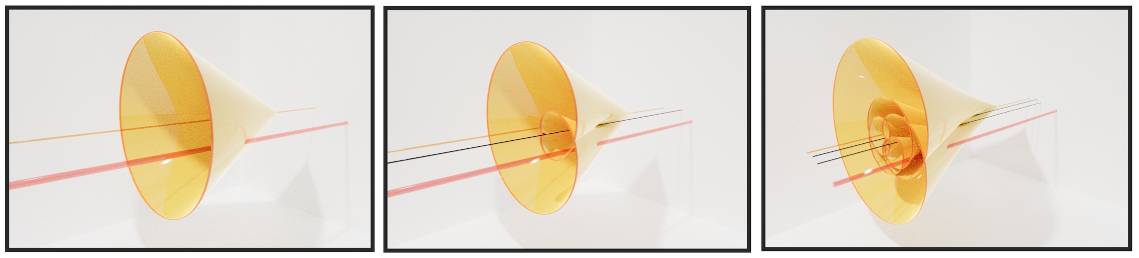
Accurately ray-tracing a scene that contains several black holes is, in principle, straightforward: follow every lightlike geodesic backward along the camera’s past light cone until it strikes an object (Figure 1). In practice however, the task explodes into solving nonlinear ODEs on a complicated spacetime (itself the solution of nonlinear PDE), an enterprise that is both fragile and computationally demanding.
In this note we exhibit a situation where these difficulties can be avoided, thanks to a beautiful exact solution to general relativity containing charged black holes in static equilibrium. Exploiting its symmetries with tricks of Lorentzian geometry, we reduce the null-geodesic equation to a three-dimensional system corresponding to light rays in flat space with variable optical media. This allows the exact rendering of black holes in a Euclidean rendering engine with advanced optics - no relativistic simulator required. As examples, all figures were produced with my custom renderer, by implementing variable indices of refraction.

A Standoff between Electromagnetism and Gravity
Einstein’s field equation is a system of 10 coupled, nonlinear partial differential equations governing the interplay between spacetime geometry and matter. Solutions describing single black holes have been known since the theory’s inception, but finding multiple black hole solutions is far more challenging as gravitational attraction leads to rapid orbits, energy loss via gravitational waves, and eventual mergers. The strong nonlinearities of Einstein’s equations typically make such spacetimes difficult even with advanced numerics.
Happily there is a beautiful exception to this general rule. In 1947, Mamjudar and Papapetrou [3] discovered a remarkably simple exact solution to the vacuum Einstein Maxwell equations: given a harmonic function on , the metric is a solution111Throughout, we write for the Euclidean line element . for the electrostatic potential . Later in 1972 Hartle and Hawking showed these solutions include descriptions of multiple charged black holes [1], henceforth MP Black Holes. Precisely, the potential represents a single extremally charged black hole (with unit mass and charge, in natural units), and linear combinations represent a collection of extremal black holes of mass=charge at coordinate positions 222The points actually represent the event horizons: following Hartle & Hawking, one must change coordinates and analytically continue to represent the black hole interiors. But for the tracing light to an external observer, these coordinates are sufficient.. This solution is remarkably simple: its static, so the presence of multiple black holes does not lead to gravitational waves or mergers. The secret lies in a precise balancing act, with gravitational attraction exactly canceled by electrostatic repulsion.
When Gravity Acts Like Glass
Starting from this exact solution, we apply results from Lorentzian geometry to simplify the calculations required for tracing light rays. Our key trick is that for computing null geodesics (paths which travel at the speed of light), its often possible to swap out the given spacetime with a simpler one. Formally:
Proposition: Null geodesics are invariant under a conformal rescaling of the metric.
We sketch the proof for the interested reader’s benefit: let be a null geodesic of , and a conformal rescaling. Note is still a null curve for as . Computing we see its not turning (acceleration is parallel to velocity), but is not constant speed. Changing speed via reparameterization for , we see (after some algebra) that , and so taking to solve the differential equation makes a null geodesic. But traces the same curve in spacetime as , QED.
Consequence: The trajectories of light around the extremal black holes described by are identical to the null geodesics of (the result of a conformal rescaling by ).
This new metric is much simpler: represents proper time for all stationary observers. Time’s uniform flow renders it inessential to the dynamics, and we lose no information projecting onto their spatial shadows.
Proposition: Null geodesics of on project to Riemannian geodesics of .
Consequence: Let . Then the light ray of the MP black hole metric originating at in direction hits the world-tube if and only if the geodesic of with initial data intersects .
Thus for static objects (whose worldlines are also unchanging in ), this reduces the entire relativistic raytracing problem to three dimensions. And a final beautiful insight remains hidden in the particular form of this three dimensional system. Re-interpreting the distance computed via arclength integral as time, we invoke Fermat’s principle to recognize these as light trajectories in classical physics.
Proposition: Geodesics of the Riemannian metric on are precisely the trajectories of light in classical physics passing through a medium with index of refraction in Euclidean space .
Putting everything together, we have proven the following rather remarkable correspondence:
Theorem: Raytracing static objects in the MP black hole system with metric is equivalent to tracing objects in flat space, immersed in a medium of refractive index .
Note this is a special property of MP black holes: applying the same tricks to the Schwarzschild metric projects light to the geodesics of on (in spherical coordinates), but this metric is not conformal to the flat metric , so these are not the light rays of a classical system.

Building a Renderer
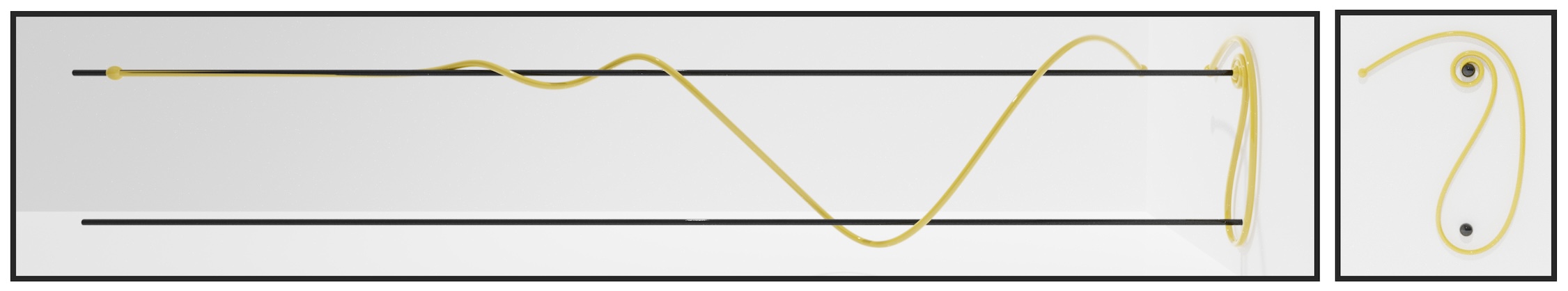
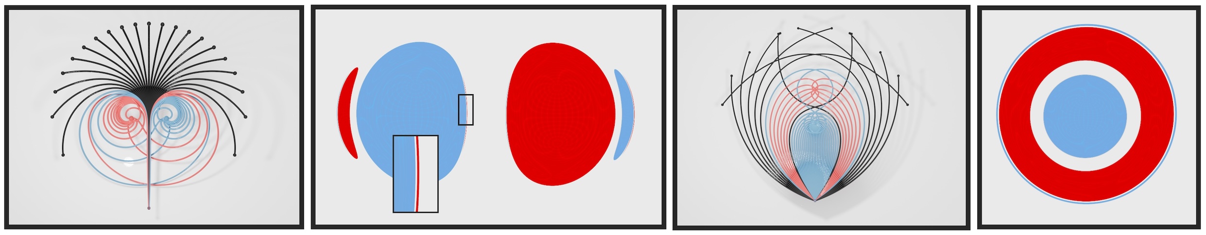
As a result, any renderer capable of supporting spatially varying refractive indices can accurately depict charged black holes, by filling a region with optical medium of index : see Fig. 4 for my own implementation. You can also fully convert a Euclidean renderer to a MP black hole renderer (as I did for Figs. 2 and 5). First replace affine rays with numerically integrated geodesics of the metric . Then replace the tracing / raymarching loop with a simple check for object intersections at each integration step. And that’s it! As is conformally flat, its inner product is a multiple of the standard inner product. So normals, reflections and refractions—anything using normalized dot products — carry over unchanged. For those wanting to modify a hobby renderer, we give the precise ODEs for the geodesic flow below.
Proposition: The trajectories of light in an optical medium with index of refraction solve the differential equation .
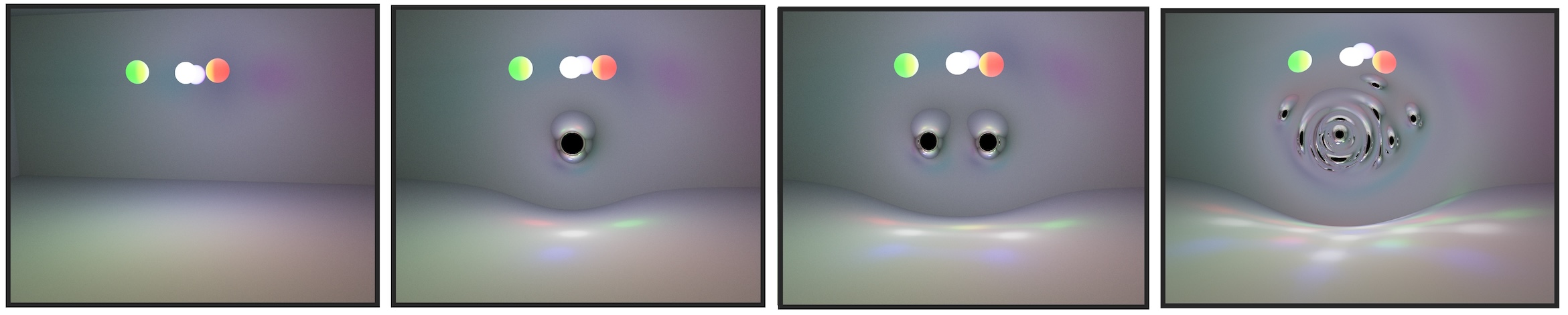
After this hard work we treat ourselves to an image of gravitational lensing: like more familiar caustics in path tracing, convergence requires many samples, but the result is stunning for multi-black hole spacetimes.
Black Hole Shadows
These techniques also allow real-time rendering of black hole shadows (or event horizons, as viewed by a distant observer). There is a collection of papers on the chaotic dynamics of light in these MP black hole spacetimes (see [2] for a readable introduction) whose results we can illustrate, by tracing light rays forward from the screen and coloring pixels according to which black hole they fall into. Figure 6 gives two perspectives on a binary system, and Figure 7 shows several levels of zoom on a six black hole system.

Summary & Acknowledgements
This work highlights a correspondence between light propagation in Majumdar-Papapetrou black hole spacetimes and classical optics in a variable refractive medium. By leveraging this analogy, we transform the challenge of relativistic ray tracing into a problem solvable with standard 3D graphics techniques, enabling efficient and accurate visualization of complex black hole configurations. I would like to thank Marcelo Seri for introducing me to the beautiful Majumdar Papapetrou solution, which started this project.
References
- [1] J. B. Hartle and S. W. Hawking. “Solutions of the Einstein-Maxwell equations with many black holes.” Commun. Math. Phys., vol. 26, 1972, pp. 87–101.
- [2] M. Kluitenberg, D. Roest, and M. Seri. “Chaotic light scattering around extremal black holes.” Bollettino dell’Unione Matematica Italiana, vol. 16, 2023, pp. 381–396.
- [3] S. D. Majumdar. “A class of exact solutions of Einstein’s field equations.” Physical Review, vol. 72, no. 5, 1947, pp. 390–398.