Axion Dark Matter Archaeology with Primordial Gravitational Waves

Abstract

We investigate the complementary information to be gained from inflationary gravitational wave (IGW) signals and searches for QCD axion dark matter. We focus on post-inflationary Peccei-Quinn (PQ) breaking axion models that are cosmologically safe. Recent work has shown that a greater number of such models exist. This is because the heavy quarks required for the colour anomaly can provoke a period of heavy quark domination (HQD), which, through decay, dilutes the axion abundance. In this work we show for the first time that the axion dark matter mass can be as low as $m_{a}\sim 10^{-8}\,{\rm eV}$ for models where the heavy quarks decay via dimension 6 terms. This is achieved by allowing the mass of the heavy quarks to differ from the axion decay constant, $m_{Q}\neq f_{a}$. Consequently, the observables that would distinguish between pre- and post-inflationary PQ breaking, $m_{a}$ and the additional relativistic degrees of freedom $\Delta N_{\rm eff}$, now become indiscernible. To solve this, we propose using blue-tilted IGWs to probe HQD. By leveraging the features of the GW signal, future interferometers can probe $m_{Q}$ and $f_{a}$ complementing the sensitivity of haloscope experiments, potentially pinning down all relevant parameter that describe the physics. Specifically, we find that BBO and ET GW detectors will both be able to optimistically probe $f_{a}\gtrsim 10^{14}\,{\rm GeV}$.

1 Introduction

The QCD axion provides a compelling an elegant explanation of both the strong CP problem and dark matter simultaneously. The axion itself is the proposed pseudo-Nambu-Goldstone boson of a new spontaneously broken $U(1)_{\rm PQ}$ symmetry [1, 2, 3, 4]. As a consequence the axion’s mass, $m_{a}$, can naturally be very light and can be related to the breaking scale $f_{a}$ via

$$m_{a}=5.7\times 10^{-5}\,{\rm eV}\left(\frac{10^{11}\,{\rm GeV}}{f_{a}}\right).$$ (1.1)

Such a light boson in an expanding Universe will undergo a non-thermal production mechanism known as vacuum misalignment [5, 6, 7] (see also reviews in Refs. [8, 9]). This mechanism produces a cold dark matter abundance of axions which can constitute all of the relic dark matter inferred from cosmology and astrophysics [10]. This implies a very high symmetry breaking scale, $f_{a}\sim 10^{11}-10^{12}\,{\rm GeV}$ with the corresponding axion mass, $m_{a}$ being $\mathcal{O}(10)\,\mu{\rm eV}$. Therefore, by searching for evidence of the axion, we will be indirectly probing physics at energy scales far beyond the reach of current particle physics colliders.

Fortunately, the solution to the CP problem necessitates some interactions between the axion and the Standard Model (SM), the strength of which is also suppressed by $f_{a}$. Despite this large suppression, axion emission from supernovae [11] as well as precision measurement of hadron decays at experiments like NA62 [12] and KOTO [13] provide lower bounds on $f_{a}$ [14, 15]. Furthermore, dedicated axion dark matter experiments such as ADMX [16, 17], CAPP [18], UF [19], TASEH [20], HAYSTAC [21] and QUAX [22, 23] have achieved excellent sensitivities, and future experiments like MADMAX [24, 25], ORGAN [26, 27], FLASH [28, 29], BabyIAXO-RADES [30], DMRadio [31] promise to survey large portions of the parameter range where QCD axion dark matter is predicted.

By probing energies far beyond the ${\rm TeV}$-scale we are indirectly exploring physics of the very early Universe, an epoch we know very little about [32]. Indeed we can only say with certainty that there was a period of cosmic inflation which ended and by the time of Big Bang Nucleosynthesis (BBN), $T\sim 3\,{\rm MeV}$, the Universe was dominated by SM radiation. This provides ambiguity about the dynamics of any high-scale extension to the SM such as the those responsible for the PQ mechanism. For example, the consequences of symmetry breaking above or below the temperature of reheating after inflation are different. If the $U(1)_{\rm PQ}$ symmetry is broken after inflation many axion models predict the formation of stable topological defects such as domain walls [33, 34], which require additional mechanisms to destroy [35, 36, 37]. Recently, it has been shown that a number of models that do not have a domain wall problem [38, 39] will generate a period of early heavy quark domination (HQD) [40, 41] akin to early matter domination (EMD). As a consequence the measurable parameters that would distinguish the pre and post-inflationary symmetry breaking scenarios are equivalent. The task is then to find additional probes on the time of $U(1)_{\rm PQ}$ breaking in relation to inflation. We show that inflationary first-order gravitational waves (GWs), in tandem with axion haloscope experiments will be able do this. We promote such tests of axion dark matter in complementary searches between laboratory and GW experiments.

In this work we focus on GWs that are generated from quantum tensor fluctuations of the metric during inflation [42, 43, 44, 45]. The spectrum of such GWs follow a simple power law during radiation domination acting as a tracer of cosmic expansion  [46, 47, 48, 49, 50, 51, 52, 53, 54, 55, 56, 57, 58]. Any departure from the standard thermal history, such as HQD provides distinctive GW spectral features  [59, 60, 61, 62, 63, 64, 65, 66]. Investigating such features reveals both the time at which early matter domination began and its duration. We will show that this allows us to get a handle on the mass of the particle responsible for HQD, and the rate of their decay. Only when combining this information with axion haloscope experiments can we determine the breaking scale $f_{a}$. We therefore show that complementarity between GW and axion experiments will be vital for reconstructing the relevant particle physics parameters.

This paper is organized as follows, in section 2 we describe effective axion model framework that we utilize in this article. We discuss how EMD is generated and show how such a scenario changes the expected value for $m_{a}$. We then discuss how this complicates phenomenological implications for pre and post-inflationary $U(1)_{\rm PQ}$ scenario. In section 3 we review the modelling of inflationary first-order GWs and how they can be used to detect a period of EMD before BBN. We also describe our limit setting methodology which we undertake for all relevant current and future GW detectors. In section 4 we present our results, combining axion haloscope and GW experiments, we discuss the current status and future potential. Finally we conclude in section 5.

2 Preferred Axion models with Heavy Quarks

The cornerstone of the Peccei-Quinn (PQ) solution [1, 2] to the strong CP (charge parity) problem is to propose a dimension-5 term, the colour anomaly, in addition to the CP violating term allowed by SM gauge invariance. These enter the Lagrangian as

$$\mathcal{L}_{\text{PQ}}\supset N\frac{a\left(t,x\right)}{f_{a}}\frac{g_{s}^{2}}{32\pi^{2}}\tilde{G}^{\mu\nu}_{b}G_{\mu\nu}+\theta\frac{g_{s}^{2}}{32\pi^{2}}\tilde{G}^{\mu\nu}_{b}G_{\mu\nu},$$ (2.1)

where $a$ is the axion field, $G$ and $\tilde{G}$ are the field strength tensors of the gluon field and its dual respectively. The coefficients $g_{s}$, $\theta$, $N$, and $f_{a}$ are the SM strong coupling constant, the QCD vacuum angle, a model-dependent anomaly coefficient, and the axion decay constant respectively. The first term, under the influence of the QCD potential is dynamically driven to cancel the second term, resulting in no detectable CP violation from strong interactions. How this dimension-5 operator is generated is a model building exercise. Typically there are two approaches: either with SM particles charged under the new $U(1)_{\rm PQ}$ (DSFZ-type [67, 68, 69]) or not (KSVZ-type [70, 71]). In both cases new particles are required, for KSVZ, the minimal requirement is to introduce two new fields: a new $SU(3)_{c}$ charged fermion, $Q$, a heavy quark; and a complex scalar field $\Phi$ which drives the PQ breaking. The PQ Lagrangian is given by

$$\mathcal{L}_{\rm PQ}=|\partial_{\mu}\Phi|^{2}+\overline{Q}i\not{D}Q-(y_{Q}\overline{Q}_{L}Q_{R}\Phi+{\rm H.c.})\,.$$ (2.2)

Where $y_{Q}$ is the BSM Yukawa coupling which generates Q mass when PQ symmetry is broken. The PQ charge of $\Phi$ is $1$ and the chiral left-handed $Q_{L}$ and right-handed $Q_{R}$ fields have different charges $\chi_{L}$ and $\chi_{R}$ respectively, but with $|\chi_{L}-\chi_{R}|=1$ such that the above Lagrangian is symmetric under $U(1)_{\rm PQ}$. In the broken phase, the Yukawa term reduces to a mass term with $m_{Q}=y_{Q}f_{a}/\sqrt{2}$. If the breaking scale is below the reheating temperature of the early Universe, $T_{\rm PQ}<T_{\rm RH}$, then the strongly charged $Q$ particles will initially be in thermal equilibrium with the SM plasma. After PQ breaking, the heavy quarks acquire a mass and will freeze-out. As pointed out in Refs. [38, 39], performing standard thermal production would generate a large relic abundance of heavy quarks, violating constraints from cosmology unless they decay quickly enough.

Furthermore, the misalignment mechanism generates a cold axion abundance [5, 6, 7, 72]:

$$\Omega_{a}h^{2}\approx 0.12\,\left(\frac{\theta_{\rm i}}{2.15}\right)^{2}\left(\frac{28~\mu{\rm eV}}{m_{a}}\right)^{7/6},$$ (2.3)

where $\theta_{i}$ is the initial angle of the field, $\theta=a/f_{a}$, which for the $U(1)_{\rm PQ}$ breaking after inflation is approximated to be $\theta_{i}\approx 2.15$. This number is obtained by accounting for multiple Hubble patches undergoing misalignment with an ensemble of $\theta_{i}$ values [73]. This then limits the axion mass to be $m_{a}\,\gtrsim 15\,\mu{\rm eV}$ in order to avoid axion overproduction.

Combining this with the need for fast $Q$ decays, authors of Refs. [38, 39] utilized an effective field theory approach as a guide on what axion models are compatible with standard cosmology, heavy quark decay terms are described by

$$\mathcal{L}_{Qq}=\mathcal{L}_{Qq}^{d\leq 4}+\mathcal{L}_{Qq}^{d>4}=\mathcal{L}_{Qq}^{d\leq 4}+\frac{1}{\Lambda^{(d-4)}}\mathcal{O}^{d>4}+{\rm h.c.}\,.$$ (2.4)

where $d$ is the mass dimension of the operators. Taking the cut-off scale as the Planck scale $\Lambda=m_{\rm Pl}=1.22\times 10^{19}\,{\rm GeV}$, it was found that the maximum dimension for decay while avoiding the overproduction of axions was $d=5$. However, recently Ref. [40] found that for decays $d\geq 5$, the thermally produced heavy quarks will provoke a period of heavy quark domination (HQD), altering the misalignment mechanism in such a way as to allow for smaller axion masses and larger dimension for $Q$ decay. A period of early matter domination altering the dynamics of the misalignment mechanism has been explored before [74, 75, 76, 77, 78, 79, 80, 81, 82, 83], typically by introducing additional matter content as new physics. Ref. [40] on the other hand pointed out that for KSVZ axion models, the additional matter content is already present. This result means that a greater number of axion models are viable, in Ref. [41] authors enumerate such models. Notably, they found that there are four $d=6$ and two $d=9$ SM charge assignment for the heavy quark that do not suffer from a domain wall problem, this extends the previously known two, KSVZ-I and KSVZ-II, to eight.

2.1 Condition for heavy quark domination

Here we describe in more detail the thermal freeze-out and later early matter domination of the heavy quarks. The $\bar{Q}+Q\to{\rm SM}+{\rm SM}$ annihilation cross-section is given by

$$\langle\sigma v\rangle_{\bar{Q}Q}=\frac{\pi\alpha_{s}^{2}}{16m_{Q}^{2}}\left(c_{f}n_{f}+c_{g}\right).$$ (2.5)

where $n_{f}$ is the number of quark flavors that $Q$ can annihilate into, and $\left(c_{f},c_{g}\right)=\left(2/9,\,220/27\right)$ for triplets and $\left(c_{f},c_{g}\right)=\left(2/3,\,27/4\right)$ for octets, in this paper we assume the former. Through the standard thermal freeze-out procedure one can determine the temperature of the SM plasma when $\rho_{Q}\approx\rho_{\rm SM}$ [40],

$$T_{\rm dom}\approx 10^{7}\left(\frac{m_{Q}}{10^{12}\,\text{GeV}}\right)^{2}\,\text{GeV}.$$ (2.6)

In order for heavy quarks to dominate the early Universe, their decay must occur after heavy quark-radiation equality. Since the plasma temperature is always decreasing, we require $T_{\rm decay}<T_{\rm dom}$. To estimate $T^{Q}_{\rm decay}$, we set $\Gamma_{Q}\equiv H_{\rm rad}\left(T=T^{Q}_{\rm decay}\right)$ where $H_{\rm rad}$ is the Hubble parameter in the radiation-dominated Universe,

$$T_{\rm decay}^{d}=\left(\Gamma^{d}_{Q}\right)^{\frac{1}{2}}\left(\frac{1}{g_{\star}(T_{\rm decay})}\right)^{\frac{1}{4}}\left(\frac{90\,m_{\rm Pl}^{2}}{8\pi^{3}}\right)^{\frac{1}{4}}.$$ (2.7)

Where $g_{\star}$ is the effective energy degrees of freedom. The decay widths of $Q$ for each dimension of decay is

$$\Gamma^{d=4}_{Q} =\frac{m_{Q}}{8\pi},\,\,\,\, \Gamma_{Q}^{d=5} =\frac{m_{Q}^{3}}{16\pi\Lambda^{2}},$$

$$\Gamma_{Q}^{d=6} =\frac{m_{Q}^{5}}{512\pi^{3}\Lambda^{4}},\,\,\,\, \Gamma_{Q}^{d=7} =\frac{m_{Q}^{7}}{49152\pi^{5}\Lambda^{6}},\,$$ (2.8)

where we neglect the details of higher dimension decays in this paper. Furthermore, the main focus in this article will be the dimension 6 and 7 dimensional decay terms. This is because $d\leq 5$ models will not produce periods of HQD that will alter the misalignment mechanism. Models with $d=5$ decays can lead to HQD, but these typically require $m_{Q}>f_{a}$ or predict overproduction of the axion due to a large $f_{a}$ and has no in-built mechanism to dilute it. Using Eq. (2.8) one can estimate when $T_{\rm dom}>T_{\rm decay}$. For $d=6$ and $d=7$, this is when

$$\Lambda\gtrsim(4\times 10^{28}\,{\rm GeV}^{2}\,\times m_{Q}M_{\rm Pl})^{1/4}\,\,\,\,{\rm and}\,\,\,\,\Lambda\gtrsim(4\times 10^{25}\,{\rm GeV}^{2}\,\times m_{Q}^{3}M_{\rm Pl})^{1/6},$$ (2.9)

respectively. Furthermore, with the calculation of $T_{\rm dec}$ we are able to assess whether a particular model and parameter point is in tension with BBN [84, 85, 86, 87]. Typically one estimates this by checking that $T_{\rm dec}\gtrsim 3\,{\rm MeV}$.

2.2 Axion misalignment with heavy quark domination

The details of the axion misalignment mechanism within non-standard cosmologies can be found in Refs. [74, 75, 76, 77, 78, 79, 80, 81, 88]. The insight of Ref. [40] was that axion models themselves typically contain all necessary ingredients for early matter domination.

The full dynamics are determined by the coupled Friedmann Boltzmann equations

$$\frac{3H^{2}M_{\rm Pl}^{2}}{8\pi} = \rho_{\mathrm{R}}^{\rm SM}+\rho_{Q}\,,$$ (2.10a)

$$\frac{\differential s_{\mathrm{R}}^{\rm SM}}{\differential t} = -3Hs_{\mathrm{R}}^{\rm SM}+\frac{{\rm BR}_{\rm SM}\Gamma_{Q}}{T}\rho_{Q}\,,$$ (2.10b)

$$\frac{\differential n_{Q}}{\differential t} = -3Hn_{Q}-\Gamma_{Q}n_{Q}-\langle\sigma\,v\rangle\left[n_{Q}^{2}-(n_{Q}^{\rm eq})^{2}\right]\,,$$ (2.10c)

where $\rho$, $n$ and $s$ are the energy, number, and entropy densities respectively, we also denote each component, SM radiation (R), heavy quark ($Q$), in the subscript. Note that we haven’t included the Boltzmann equation for the the thermally produced axion. As shown in Refs. [40, 89], if HQD occurs, the branching ratio to axions must be subdominant otherwise axion contributions to $\Delta N_{\rm eff}$ would be too large. Hence, in this work we only consider 100% decay into SM particles, which implies that if HQD occurs and ends after thermal axion decoupling, then $\Delta N_{\rm eff}$ will be much less than the expected value from the standard thermal axion, i.e. $\Delta N_{\rm eff}\ll 0.027$. This is despite the axion actually having been in thermal contact with the SM early on.

One can solve Eqs. (2.10) to validate the approximations made in Eq. (2.6) and Eq. (2.7), and to when generate the GW signals in section 3. We use the precise determination of $H$ as an input to solve the misalignment mechanism using the dedicated solver MiMeS [90]. Specifically, we solve the equation of motion for the axion field, $a$, which is expressed in terms of the axion angle, $\theta=a/f_{a}$

$$\left(\frac{\differential^{2}}{\differential t^{2}}+3H(t)\frac{\differential}{\differential t}\right)\theta(t)+\tilde{m}_{a}^{2}(t)\sin(\theta(t))=0\,,$$ (2.11)

where $\tilde{m}_{a}(t)$ is the thermal mass of the axion [91]. Generically, the axion abundance is diluted such that a greater $f_{a}$ is required to achieve the correct relic abundance for axion dark matter.

In order to make the connection with the experimental search for axion dark matter, we numerically solve Eqs. (2.10) and Eq. (2.11) to find the required $f_{a}$ such that $\Omega_{a}\,h^{2}=\Omega_{\rm DM}\,h^{2}$, where we take the relic abundance of dark matter determined in [92]. We do this for a range of $m_{Q}$ and $\Lambda$ values, and take $\theta_{i}=2.15$ in-line with calculations of post-inflationary PQ breaking [73]. Furthermore, we check that $\rho_{\rm R}>\rho_{Q}$ at the onset of BBN. In previous works $m_{Q}\sim f_{a}$ and $\Lambda\sim m_{\rm Pl}$ were taken, but these are simply the upper bounds on such parameters, we find that by insisting that the QCD axion has to account for all of the dark matter, these assumptions can be relaxed and we still have a sufficiently constrained scenario.

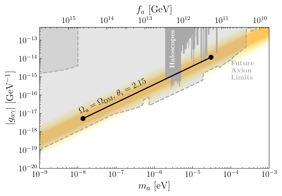
Figure 1: The range of axion mass $m_{a}$ which can reproduce the correct relic abundance allowing for any $m_{Q}\lesssim f_{a}$ and $\Lambda<m_{\rm Pl}$. This is for $d=6$ but we find the result for $d=7$ decays to be very similar. The axion limits and QCD axion band was plotted using Ref. [93].

Fig. 1 shows the range of $m_{a}$ values that can achieve the correct relic abundance, allowing $m_{Q}$ and $\Lambda$ to vary. We have presented the possible $m_{a}$ range in the $\left(m_{a},g_{a\gamma}\right)$-plane, where $g_{a\gamma}$ is the axion-photon coupling which depends on the anomaly coefficients, $N$, from Eq. (2.1) and $E$, the coefficient of the electromagnetic anomaly term,

$$g_{a\gamma}\equiv\frac{\alpha}{2\pi}\frac{1}{f_{a}}\left(\frac{E}{N}-1.92(4)\right).$$ (2.12)

$\alpha$ is the electromagnetic fine-structure constant. In this article, we remain agnostic about the specific axion model and therefore show a representative line for $E/N=0$. Furthermore, the yellow band shows a model independent band encompassing most QCD axion models. We note that by allowing $m_{Q}\lesssim f_{a}$ we have found a substantial quantitative difference from the results in Refs. [40, 41] where models with $d=6$ decay terms were found to only marginally change the expected $m_{a}$ value that reproduces the correct relic density, even when $\Lambda$ could vary. In Fig. 1 we see that $d=6$ decays can alter the cosmology such that the $f_{a}$ required for $\Omega_{a}\,h^{2}=\Omega_{\rm DM}\,h^{2}$ is orders of magnitude higher. What limits this value is the constraints from BBN. The left most point on the axion dark matter line corresponds to $f_{a}=4\times 10^{14}\,{\rm GeV}$, $m_{Q}=4\times 10^{11}\,{\rm GeV}$, and $\Lambda=4\times 10^{18}\,{\rm GeV}$. Calculating $T_{\rm dec}$ via Eq. (2.7) gives $5\,{\rm MeV}$, but due the more precise numerical evaluation from Eq. (2.10) gives $T_{\rm dec}=3\,{\rm MeV}$.

We show this slight difference in the way we calculate the constraint from BBN on the $\left(m_{Q},\Lambda\right)$-plane in Fig. 2. The black and white hatched region is bounded by a dotted and a solid line, which indicates the approximate bound (Eq. (2.7)) or full numerical one (Eqs. (2.10)) respectively. One can see the constraints coming from the more accurate numerical evaluation is more aggressive, henceforth the BBN bounds we will show correspond to this. All the points in Fig. 2 to the right of the hatched region can satisfy $\Omega_{a}=\Omega_{\rm DM}$ given the certain choice of $f_{a}$. Some of those $f_{a}$ values will coincide with the haloscope experiment constraints shown in Fig. 2 as a dark gray region. In particular, the two experiments that have reached sensitivities down to the KSVZ line in the relevant $f_{a}$ region is ADMX [16, 94] and CAPP [95, 96, 18, 97], they are the crimson red and orange in shaded regions in Fig. 2. Note that since these experiments are haloscope experiments, their sensitivity is intimately tied to the $\Omega_{a}=\Omega_{\rm DM}$ requirement we made. In the left panel of Fig. 2 we show the results for $d=6$ decay terms, and in the right panel we show the results for $d=7$ decay terms. This will be useful in assessing the potential for future GW experiments to probe the same parameter space. As we will show in section 3, the inflationary GW signal is sensitive $m_{Q}$ and $\Lambda$ and not $f_{a}$ directly.

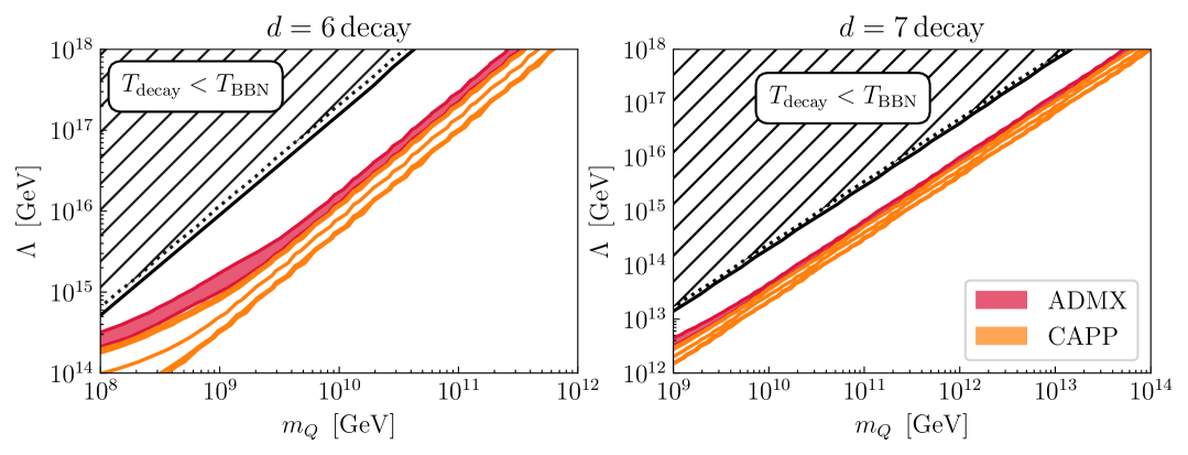
Figure 2: The current constraints on the $m_{Q}$ and $\Lambda$ parameter space from ADMX and CAPP experiments. The left panel is for $d=6$ decays and the right panel is for $d=7$ decays. The value of $f_{a}$ is not a priori set, instead we determine the required value such that $\Omega_{a}=\Omega_{\rm cdm}$. The hatched region is where $Q$ decay occurs too late and will be constrained by BBN, we have bounded it by the dotted and solid black lines which correspond to the more approximate Eq. (2.7) and precise numical evaluation via Eqs. (2.10) respectively.

Before we move on, we comment that we have not included any contribution to the axion abundance from topological defects such as cosmic strings or unstable domain walls [98, 99, 100]. We do this because the exact contribution is still under dispute in the literature and all calculations to date have been performed under standard cosmology [101, 102, 103, 104, 105, 106, 107]. Furthermore, since the vast majority of the axion abundance is produced around the QCD phase transition $T_{\rm QCD}$, similarly to the misalignment mechanism, the effect where HQD dilutes the axion abundance will also hold. Future work is warranted in this direction, but it is beyond the scope of this article.

2.3 Interpreting the cosmology of a low mass axion

In the previous subsection we have shown that axion models with post-inflationary PQ breaking can lead to axion dark matter with masses as low as $\sim 10^{-8}\,{\rm eV}$. The only requirements are that the new particles that generate the anomaly term in Eq. (2.2), are heavy ($m_{Q}\gtrsim 10^{7}\,{\rm GeV}$) and live long enough. For the effective parametrisation of Eq. (2.4), this translates to the requirement that the lowest dimension decay terms have to be $d\geq 6$. What’s more, recently Ref. [41] found that there exists four dimension 6 KSVZ-type charge configurations that do not have a domain wall problem, for lower dimensions, there are only two configurations. Additionally, it appears that these new models contain $Q$ decays to SM particles only, therefore $\Delta N_{\rm eff}\ll 0.027$ [89].

This poses an interesting problem for distinguishing between the pre- and post-inflationary PQ breaking scenarios because now both possibilities can easily produce the same values for $m_{a}$ and $\Delta N_{\rm eff}$. What’s more, the pre-inflationary $U(1)_{\rm PQ}$ breaking case typically requires a finely tuned initial angle $\theta_{i}\ll 1$ to produce axion dark matter with masses $m_{a}\lesssim 10^{-6}\,{\rm eV}$. In the context of post-inflationary breaking we presented above, fine-tuning comes in via small Yukawa couplings, $y_{q}\sim 10^{-3}$, well within the range observed in the SM, so shouldn’t cause much theoretical consternation.

As always, we would like to find experimental avenues to break the degeneracy between the pre and post-inflationary breaking scenario. What’s more, some kind of understanding of when $U(1)_{\rm PQ}$ breaking occurred relative to the reheating temperature would constitute a profound insight into the nature and scale of inflation. As we’ve seen in Eq. (2.6) and Eq. (2.8) the onset and end of HQD is sensitive to fundamental parameters of the underlying theory, so if we can probe these events experimentally in some way, we will be able to learn about the possible axion models. As we will see in the next section, inflationary gravitational waves may provide precisely this insight.

3 Primordial Gravitational Waves

An early matter domination epoch, occurring within post-reheating and pre-BBN era leaves distinct imprints on stochastic gravitational wave background. Here we will explore how the HQD influences the GW spectrum, examining the unique features it induces. GWs generated during inflation exhibit constant amplitudes outside the horizon and undergo damping upon re-entry. At the present epoch, the observed GW spectrum, $\Omega_{\text{GW}}(k)$, can be expressed in terms of wave-number ($k$) as

$$\Omega_{\text{GW}}(k)=\frac{1}{12}\left(\frac{k}{a_{0}H_{0}}\right)^{2}T_{T}^{2}(k)\;P_{T}^{\text{prim}}(k),$$ (3.1)

with $a_{0}(H_{0})$ being the Friedmann-Lemaitre-Robertson-Walker (FLRW) metric scale factor (Hubble parameter) at the present time [63]. $P_{T}^{\text{prim}}$ represents the primordial power spectrum from inflation which can be expressed as [108, 109, 110, 111, 112, 113, 114]

$$P_{T}^{\text{prim.}}(k)=A_{T}(k)\left(\frac{k}{k_{\ast}}\right)^{n_{T}}.$$ (3.2)

$A_{T}$ represents the amplitude of the tensor power spectra and determines the amplitude of the GW spectrum. It is evaluated at a particular pivot scale $k_{\ast}=0.05$ Mpc^-1, where the Planck collaboration reports its observational constraints [92]. Additionally, $n_{T}$ is the tensor spectral index, which governs the tilts of the GW spectrum. A positive $n_{T}$ corresponds to a blue-tilted spectrum, while a negative $n_{T}$ leads to red-tilted spectrum. Although standard single-field slow-roll inflation generally predicts a red-tilted $n_{T}$ [115], several alternative scenarios can produce a blue-tilted $n_{T}$ spectrum, for instances, string cosmology [116, 117], modified gravity [118], particle production during inflation [119, 120], G-inflation [121], Higgsed chromo-natural inflation [122], natural inflation on steep potentials [123], super-inflation modes [124], Einstein-Gauss-Bonnet inflation [125], spectator scalar field during the inflation [126], Axion gauge field inflation [127, 128], Higgsed gauge-flation [129]. Furthermore, recent NANOGrav results have been interpreted as a blue-tilted spectrum, showing a good fit [130, 131].

Blue-tilted spectra can overproduce gravitons, that will contribute to the additional effective number of relativistic degrees of freedom, $\Delta N_{\rm eff}$ [132]

$$\int^{\infty}_{f_{\rm min}}\frac{df}{f}\Omega_{\rm GW}(f)h^{2}\;\leq 5.6\times 10^{-6}\;\Delta N_{\rm eff},$$ (3.3)

where $f_{\rm min}$ is the lower limit of integration, which is $\simeq\;10^{-10}\,(\simeq\;10^{-18})$ Hz for BBN (CMB). Current observational constraints from Planck 2018 and BAO [92], along with BBN [133], place stringent upper bounds on $\Delta N_{\rm eff}$. Future CMB experiments, including CMB Bharat [134], CMB-S4 [135, 136], PICO [137], CMB-HD [138], COrE [139], the South Pole Telescope [140], and the Simons Observatory [141], are expected to further refine these constraints with improved sensitivity. Among current observations, Planck 2018+BAO provides one of the most stringent upper bounds on $\Delta N_{\rm eff}$, limiting it to $0.28$ [133]. Looking ahead, CMB-HD is projected to significantly improve this constraint, reaching a sensitivity of $0.027$ [138]. In this study, we incorporate both the current Planck 2018+BAO limit and the projected CMB-HD constraint to analyse their implications.

$T_{T}(k)$ in Eq. (3.1) is the transfer function describing the evolution of gravitational waves throughout different epochs, in the background of a FLRW Universe. In general, it can be expressed as [142, 143, 144, 50, 145, 146]:

$$T_{T}^{2}(k)\equiv\Omega_{m}^{2}\left(\frac{g_{*}(T_{\text{in}})}{g_{*}^{0}}\right)\left(\frac{g_{*S}^{0}}{g_{*S}(T_{\text{in}})}\right)^{\frac{4}{3}}\left(\frac{3j_{1}(z_{k})}{z_{k}}\right)^{2}F(k),$$ (3.4)

where $g_{\star\,S}$ is the total number of entropy degrees of freedom and $\Omega_{m}(=0.31)$ is the total matter density [92]. $j_{1}(z_{k})$ is the first order spherical Bessel function, with $z_{k}\equiv k\tau_{0}$, where $\tau_{0}=2/H_{0}$ [63, 92] being the conformal time today. Now, the imprints of any non-standard evolution during the pre-BBN epoch are encapsulated within $F(k)$. In the standard scenario (i.e. only radiation domination after inflationary reheating and before BBN), $F(k)$ has the following form:

$$F(k)\bigg{|}_{\text{standard}}\equiv T_{1}^{2}\left(\frac{k}{k_{\text{eq}}}\right)T_{2}^{2}\left(\frac{k}{k_{\text{RH}}}\right),$$ (3.5)

where $k_{\rm eq}$ and $k_{\rm RH}$ correspond to modes that reenter horizon at matter-radiation equality and the end of reheating respectively,

$$k_{\text{eq}} = 7.1\times 10^{-2}\Omega_{m}h^{2}\,{\rm Mpc}^{-1},$$ (3.6)

$$k_{\text{RH}} = 1.7\times 10^{14}\left(\frac{g_{*S}(T_{\rm RH})}{g_{*S}^{0}}\right)^{\frac{1}{6}}\left(\frac{T_{\rm RH}}{10^{7}\;\text{GeV}}\right)\,{\rm Mpc}^{-1}.$$ (3.7)

In the case of HQD, $F(k)$ becomes

$$F(k)\bigg{|}_{\text{HQD}}\equiv T_{1}^{2}\left(\frac{k}{k_{\text{eq}}}\right)T_{2}^{2}\left(\frac{k}{k_{\text{dec}}}\right)T_{3}^{2}\left(\frac{k}{k_{\text{dec, S}}}\right)T_{2}^{2}\left(\frac{k}{k_{\text{RH, S}}}\right),$$ (3.8)

where $k_{\text{dec}}$ corresponds to the wave-number at the end of HQD, estimated as

$$k_{\text{dec}} =1.7\times 10^{14}\left(\frac{g_{*S}(T_{\rm dec})}{g_{*S}^{0}}\right)^{\frac{1}{6}}\left(\frac{T_{\rm dec}}{10^{7}\;\text{GeV}}\right)\,{\rm Mpc}^{-1}.$$ (3.9)

The characteristic wave-numbers $k_{\text{dec, S}}$ and $k_{\text{RH, S}}$, in Eq. (3.8) can be expressed as

$$k_{\text{dec, S}} \equiv k_{\text{dec}}\Delta_{s}^{2/3},$$ (3.10)

$$k_{\text{RH, S}} \equiv k_{\text{RH}}\Delta_{s}^{-1/3},$$ (3.11)

where $\Delta_{s}$ is the entropy dilution factor which quantifies the the change of comoving entropy density due to the decay of the heavy quark. It is defined as the ratio of comoving entropy density after HQD to that before its onset, i.e., $\Delta_{s}\equiv S(T_{\rm dec})/S(T_{\rm dom})$. To accurately determine this dilution factor, we numerically solved the coupled Friedmann Boltzmann equations, given in Eqs. (2.10), ensuring a precise treatment of the entropy evolution throughout the process.

The fitting functions ($T_{1}^{2}(x),T_{2}^{2}(x)$ and $T_{3}^{2}(x)$) in Eq. (3.4) can be expressed as [146]

$$T_{1}^{2}(x) \equiv 1+1.57x+3.42x^{2},$$ (3.12)

$$T_{2}^{2}(x) \equiv (1-0.22x^{3/2}+0.65x^{2})^{-1},$$ (3.13)

$$T_{3}^{2}(x) \equiv 1+0.59x+0.65x^{2}.$$ (3.14)

Hence, using the above set of equations we can estimate the nature of GW spectra for the different axion parameters, leading to the HQD epoch.

3.1 GW Detection prospects with interferometers

The inflationary GW signals described in the previous subsection are yet to be detected. With the exceptional progress in GW interferometry, the prospects for observing them have significantly improved. The experimental landscape we consider can be categorized in the following way:

1. Terrestrial detectors: Laser Interferomenter Gravitational-wave Observatory (LIGO) [147, 148, 149, 150], Einstein Telescope (ET) [151, 152], Advanced LIGO (a-LIGO) [153, 154], LIGO-India [155, 156, 157, 158, 159], VIRGO [160, 161, 162, 163], advanced-VIRGO  [164, 165] [166], Cosmic Explorer (CE) [167]

2. Space based detectors: Deci-Hertz Interferometer Gravitational-wave Observatory (DECIGO) [168], Upgraded DECIGO (U-DECIGO) [169, 170, 171], Big-Bang Observer (BBO) [172, 173], Laser Interferometer Space Antenna (LISA) [174, 175], $\mu$-ARES [176].

3. Pulsar timing arrays: Square Kilometre Array (SKA) [177, 178, 179], European Pulsar Timing Array (EPTA) [180, 181, 182], North American Nanohertz Observatory for Gravitational Waves (NANOGrav) [183, 184, 185, 186, 187]

4. Cosmic microwave background radiation: Detecting BB-modes in CMB with current and future satellites. Current observational constraints from Planck 2018 [92]. Future CMB experiments include CMB Bharat [134], CMB-S4 [135, 136], PICO [137], CMB-HD [138], COrE [139], the South Pole Telescope [140], and the Simons Observatory [141].

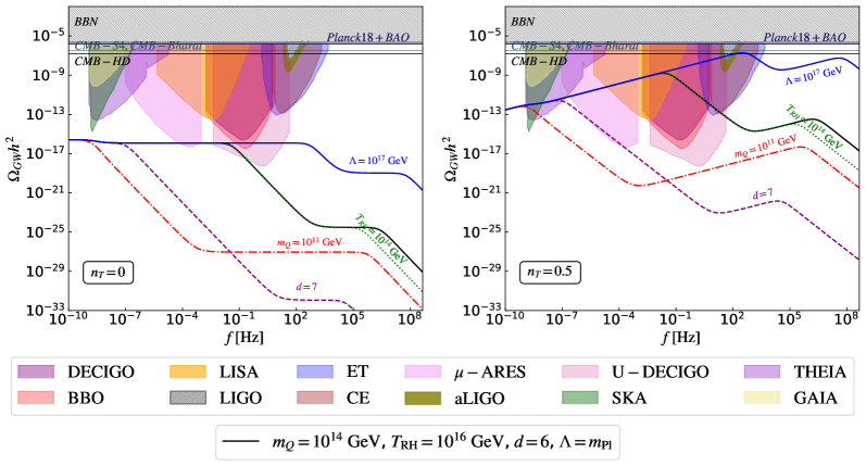
Figure 3: Illustration of GW spectrum for different values of $m_{Q}$, $d$ and $T_{\rm RH}$. In each of the GW spectrum (dashed, dot-dashed, dotted), variation with respect to parameters are quoted. Grey hatched regions are the excluded regions by the existing constraints (Plank-18+BAO, BBN and LIGO). Left panel is for $n_{T}=0$, whereas Right panel is for $n_{T}=0.5$. Here $m_{Q}$ and $T_{\rm RH}$ are in GeV. For both of the plots $r=0.036$ is fixed which corresponds to the Hubble scale of inflation $H_{\rm inf}\sim 10^{13}$ GeV.

In Fig. 3, we illustrate the behaviour the GW spectrum in presence of the HQD, as a function of frequency, assuming $r=0.036$ . The left panel of Fig. 3 corresponds to $n_{T}=0$, where the prospects of detecting the signal with current and future detectors remains low. However a blue-tilted ($n_{T}>0$) spectrum is able to enhance the detection prospects, as depicted in the right panel of Fig. 3.

Additionally, in Fig. 3, we show the power-law integrated (PLI) sensitivity curves [190] for various GW experiments, gray shaded regions are the existing bounds while rest are future sensitivty projections. These curves assume a GW spectrum varies with frequency as $\Omega_{\rm GW}\sim f^{b}$, with $b$ being the power-law exponent. The region enclosed by the PLI curve typically indicates the parameter space where a power-law signal can be detected with robust signal-to-noise ratio (SNR). Although this provides a useful benchmark, robust detection is possible only for PLI integrated curves. Therefore, we rely on a direct SNR computation to assess detectability for specific model parameters.

The PLI sensitivity curves regarding gravitational wave observatories are shown in Fig. 3. In particular, we show ground-based ET [151, 152], space-based LISA [174, 175] interferometer GW missions as well as the next generation space-based experiments like BBO [172, 173] and DECIGO [168]. We also show PTAs, including the futuristic ones like the SKA [177, 178, 179] telescope.

In both panels of Fig. 3, black solid line represents a benchmark parameter set with $m_{Q}=10^{14}$ GeV, $d=6$, $T_{\rm RH}=10^{16}$ GeV and $\Lambda=m_{\rm Pl}$. The other four curves (blue dashed, green dotted, red dot-dashed and purple short-long dashed) represent the variation of single parameters, annotated in the figure with corresponding colour, while keeping the others fixed. For instance, red dot-dashed line corresponds to $m_{Q}=10^{11}$ GeV while $d$, $T_{\rm RH}$ and $\Lambda$ remains unchanged from the black solid line. Both figures exhibit two distinct suppressions in the GW spectrum at different frequencies, where the lower one marks the periods of heavy quark decay and the higher one corresponds to inflationary reheating with $k_{\rm dec}<k_{\rm RH}$. The duration of HQD and the starting point of the suppression depend on both $T_{\rm dom}$ and $T_{\rm dec}$ where $T_{\rm dom}$ depends only on $m_{Q}$, while $T_{\rm dec}$ is affected by $m_{Q}$, $d$ and $\Lambda$. More quantitively, $f_{\rm dec}=k_{\text{dec}}/(2\pi)$, where $k_{\rm dec}$ is related to $T_{\rm dec}$ (Eq. (3.9)). At higher $k$ the GW spectrum is effected by entropy dilution until $f_{\rm dec,S}=k_{\text{dec, S}}/(2\pi)$ (Eq. (3.10)). During this period, as the Universe is dominated by matter, GW spectrum scales as $f^{-2}$. For instance, the black solid line in both figure exhibits a fall around $f=f_{\rm dec}\approx 3\times 10^{-5}\,{\rm Hz}$, which persists up to $f=f_{\rm dec,S}\approx 10$ Hz. The suppression of the GW spectrum at lower frequencies becomes more dominant as the duration of HQD increases which of course depends on $\Gamma_{Q}^{d}$. For a particular $m_{Q}$ and $d$, $\Gamma_{Q}^{d}$ decreases as $\Lambda$ increases (Eq. (2.8)) suppressing GW spectra, this can be seen in Fig. 3. By increasing $m_{Q}$ the decay rate increases as does $T_{\rm dom}$. However, the suppression becomes less for the higher values of $m_{Q}$ and $d$, as seen in Fig. 3 and understood from Eq. (2.8).

Here it is crucial to mention that PQ symmetry breaking and associated axion cosmology also leads to the formation of topological defects like global cosmic strings and domain walls which radiate GWs (see Refs.[106, 191]) and may also collapse into Primordial Black Holes [192, 193]. However, they are only relevant when PQ symmetry breaking scale $f_{a}$ is of the order of $10^{14}$ GeV or higher. This represents the upper bound of the parameter space we investigate in this article (see Fig. 11). Moreover given the period of early HQD domination such GW signals will get further suppressed leading to almost negligible signatures compared to GW from inflation that we study here, see Ref. [194, 195] for details. Nevertheless a detailed analysis of such GW analysis combined with IGW may be interesting but is beyond the scope of the present work.

3.2 Estimation of signal-to-noise ratio (SNR)

In any experimental setup, noise from several grounds affects the measured data which demands a precise characterization of the noise spectra. Thus, to quantify the prospects of signal detection in a given experiment, the SNR serves as a fundamental diagnostic tool. For any GW experiment, the SNR can be defined as [190, 196]

$${\rm SNR}\equiv\sqrt{\tau_{\rm obs}\int_{f_{\rm min}}^{f_{\rm max}}\text{d}f\left(\frac{\Omega_{\rm GW}(f,\{\theta\})h^{2}}{\Omega_{\rm GW}^{\rm noise}(f)h^{2}}\right)^{2}},$$ (3.15)

where $\Omega_{\rm GW}(f,\{\theta\})$ denotes the theoretical energy density spectrum of GW signal, characteristically parametrized by $\{\theta\}$ and $\tau_{\rm obs}$ represents the observation period of the detectors. The term $\Omega_{\rm GW}^{\rm noise}(f)$ characterizes the detector’s noise power spectral density, with $f_{\rm min}$ and $f_{\rm max}$ being the operating frequency range for GW detectors.

To ensure broad spectral coverage, we consider multiple GW detectors, including SKA, $\mu$-ARES, LISA, BBO, and ET, collectively spanning the frequency range $[10^{-9},10^{3}]$ Hz. The detailed analysis for noise characteristics of these detectors are discussed in Appendix A. For consistency in our analysis, we have adopted a uniform detection threshold of ${\rm SNR}=10$ across all GW experiments to evaluate their sensitivity to potential signals. The relevant detector specifications are summarized in Table-1.

Detectors	Frequency range	$\tau_{\rm obs}$
SKA	$\left[10^{-9}-4\times 10^{-7}\right]$ Hz	$15$ years
$\mu$-ARES	$\left[10^{-7}-1\right]$ Hz	$4$ years
LISA	$\left[10^{-4}-1\right]$ Hz	$4$ years
BBO	$\left[10^{-3}-7\right]$ Hz	$4$ years
ET	$\left[1-10^{3}\right]$ Hz	$5$ years

Table 1: Specification of the GW detectors in terms of operating frequency range and observational time period which is considered.

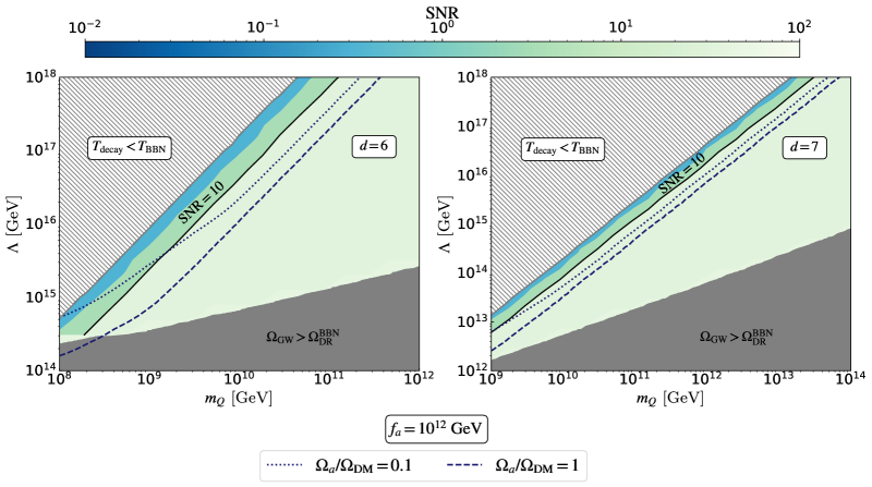
Figure 4: Illustration of SNR in the $m_{Q}-\Lambda$ plane for SKA across different dimensions. Black solid line represents ${\rm SNR}=10$, with the region below this line corresponding to ${\rm SNR}>10$, as indicated by the colour scale. The gray-shaded region denotes the parameter space excluded by BBN constraints due to the overproduction of gravitational waves. Both the dimensions are for $n_{T}=0.5$ and $r=0.036$.

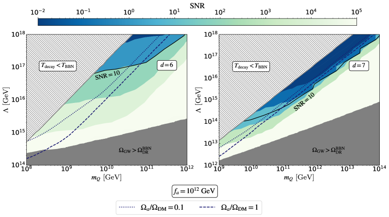
Figure 5: Descriptions of the figure is same as Fig. 4, but for $\mathbf{\mu}$-ARES.

In Figs. 4-8, we have illustrated the SNR in $m_{Q}-\Lambda$ plane, considering $d=6$ and $d=7$, for SKA, $\mu$-ARES, LISA, BBO and ET, respectively. The analysis is conducted for $n_{T}=0.5$ and $r=0.036$ to exhibit optimal sensitivity. The black and white hatched region come from BBN constraints as in section 2.2. In each figure, the black solid lines represents SNR $=10$, with the region below these lines corresponding SNR $>10$. Our findings reveal that for a given detector and specific ($m_{Q},\Lambda$) point, the SNR is generally higher for $d=6$, compared to $d=7$. This trend can be understood from the sensitivity plots which depicts that increasing the dimension strengthen the domination of early matter era, thereby reducing the detection prospect at the detectors (see, for instance, Fig. 3). Additionally, the plots indicate that SNR increases as $\Lambda$ decreases for fixed $m_{Q}$, consistently across both dimensions and all the detectors. However, the dependence on $m_{Q}$ at fixed $\Lambda$ exhibits opposite behaviour. This trend can be understood by remembering that duration of HQD which increases with increasing $\Lambda$ and decreasing $m_{Q}$. Consequently, achieving a reasonable SNR for each detector requires $\Lambda$ to be large when $m_{Q}$ is also large, a result that holds for both decay dimensions. The dark gray-shaded region in the figures corresponds to GW overproduction as determined by Eq. 3.3. Since $d=6$ results in less damping of the GW spectrum compared to $d=7$, the overproduction occurs for larger values of $\Lambda$ for $d=6$. Due to the same reason, SNR is higher for $d=6$ compared to $d=7$, for a particular $m_{Q}$ and $\Lambda$. Additionally, we observed the BBO, ET and $\mu$-ARES can probe larger $\Lambda$-values.

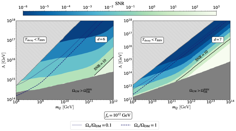
Figure 6: Descriptions of the figure is same as Fig. 4, but for LISA.

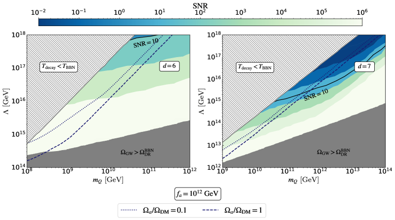
Figure 7: Descriptions of the figure is same as Fig. 4, but for BBO.

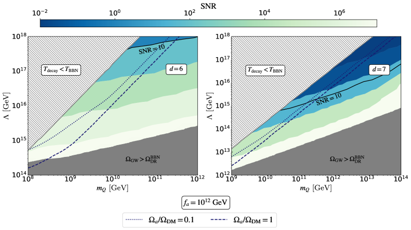
Figure 8: Descriptions of the figure is same as Fig. 4, but for ET.

Additionally in Figs. 4-8, we present the contours for the fraction of axion DM ($\Omega_{a}/\Omega_{\rm DM}$) by dark blue dotted ($10\%$) and dashed ($100\%$) lines. The contours correspond to $f_{a}=10^{12}$ GeV and are shown to indicate how a given $f_{a}$ interacts with our figures. This is important when assessing the complementary information from axion haloscopes and interferometry missions. For $d=7$ decay, GW missions are mostly sensitive for $m_{Q}$, while SKA exhibits promising detection potential to probe the axion DM across a large range of $m_{Q}$ for both dimensions. Thus, SKA, $\mu$-ARES, BBO and ET have the potential interesting regions of the post-inflationary axion scenario.

4 Axion Haloscopes and GW detectors

In the previous two sections we have shown how the effective axion model parameters $m_{Q}$, $\Lambda$, $f_{a}$ and the dimension of decay, $d$, can be inferred from axion haloscope and GW experiments separately. In this section we combine the information and explore the complementarity of the two.

4.1 Current experimental landscape

As shown in Fig. 2 and the surrounding discussion, the axion haloscope experiments CAPP and ADMX currently constrain small portions of the axion dark matter parameter space. Additionally, in section 3, we presented two existing experimental constraints that limit the parameter space for our axion models when assuming the optimistic inflationary GW background, $r=0.036$ and $n_{T}=0.5$. These are the results from Planck 2018 which limits the GW contribution to $N_{\rm eff}$ and LIGO which constrains $\Omega_{\rm GW}$ in the Hz frequency range. In Fig. 9 we present the additional GW bounds on the parameter space shown in Fig. 2. As exhibited in Figs. 4-8, GW probes are insensitive to the breaking scale $f_{a}$ as well as whether or not the misalignment mechanism produce all to dark matter. However, by fixing $\Omega_{a}=\Omega_{\rm DM}$ we can determine, for a given point on the $\left(m_{Q},\Lambda\right)$-plane, what value for $f_{a}$ is required. This in turn enables us to interpret whether a given axion haloscope experiment is sensitive to this point.

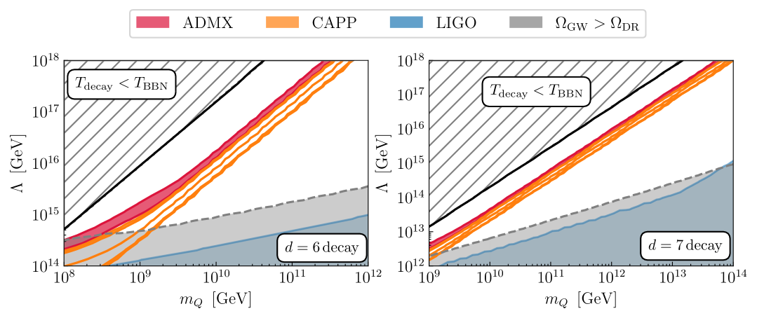
Figure 9: The same as Fig. 2 but with the limits from GWs assuming $n_{T}=0.5$ and $r=0.036$. We show the limits from LIGO and the indirect bound on $\Omega_{\rm GW}$ coming from $\Delta N_{\rm eff}$. We use the result from Planck 2018 and BAO [92].

By inspecting Fig. 9 we can see that, at least in the region of parameter space relevant for HQD, LIGO is less sensitive that constraints coming from Planck. We see in the right panel that LIGO becomes more constraining above $m_{Q}\sim 10^{14}\,{\rm GeV}$. The complementarity between experiments will become much more interesting in the near future because both axion haloscope experiments and GW detectors are set to improve substantially.

4.2 Future experimental prospects

The future GW experiments we focus on in this work are discussed in detail in section 3. The prospects for axion haloscope experiments are similarly impressive. In particular the projections of DMRadio [31], FLASH [29], BabyIAXO-RADES [30], and ADMX [94] are projected to probe substantial portions of the $m_{a}$ range that reproduce the correct relic abundance with post-inflationary PQ breaking. In Fig. 10 we only highlight DMRadio and ADMX (green shaded and red shaded regions respectively) for clarity, the sensitivities of FLASH and BabyIAXO-RADES lie in the boundary area of the two experiments shown. Overlaid we show dashed lines which present the sensitivity projections for ET (blue), LISA (magenta), $\mu$-ARES (red), SKA (green), BBO (indigo) as presented in section 3. We also show the projected sensitivities coming from improved measurements of the CMB, which will give a constraint on the additional relativistic degrees of freedom, $\Delta N_{\rm eff}$. The most sensitive of which is reported to be CMB-HD [138] (gray dashed line). We remind the reader that the SNR of each GW experiment below the SNR$=10$ line, therefore each experiment will be sensitive to parameters below the dashed lines.

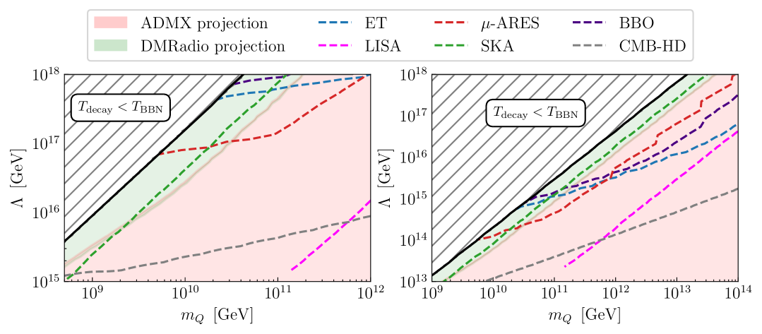
Figure 10: Future experimental landscape for axion dark matter and GW detectors. In the colored shaded regions we show the parameter regions where ADMX and DMradio a projected to be sensitive to. The dashed lines show the projected reach of future GW detectors assuming $n_{T}=0.5$ and $r=0.036$.

From Fig. 10 one can see that the DMRadio sensitivity region is closer to the $T_{\rm decay}<T_{\rm BBN}$ region, this is because DMRadio will be sensitive to lower values of $m_{a}$ (high $f_{a}$). Therefore, the misalignment production needs to be suppressed to a greater extent, which can be achieved by minimizing $T_{\rm decay}$. A later $T_{\rm decay}$ corresponds to a suppression of $\Omega_{\rm GW}$ at lower $k$ as seen in Fig. 3. The wave-number associated with $T_{\rm BBN}$ is actually lower than the SKA frequency band, therefore for such low $m_{a}$ regions that DMRadio will be sensitive to, SKA is not able to probe. Alternatively, BBO, ET and LISA will be able to probe the DMRadio regions to a greater extent. This is because shorter HQD periods allow for the blue-tilted GW spectra to reach high enough amplitudes in higher frequency bands.

We emphasise that we have chosen the parameters $n_{T}$ and $r$ in order to see the potential GW experiments have to probe high-scale axion models. Therefore the GW lines are not to be read as future constraints on the axion model, they are instead maximum sensitivity lines. In that spirit, we take all the values in the $\left(m_{Q},\Lambda\right)$-plane with ${\rm SNR}\geq 10$ for each experiment. From these points we determine the required $f_{a}$ to reproduce $\Omega_{a}=\Omega_{\rm DM}$. We take the maximum $f_{a}$ obtained and plot the result as a vertical line shown in Fig. 11. We show the $\left(m_{a},g_{a\gamma}\right)$-plane in order to make a stronger connection with axion experiments. We see that BBO, ET have the greatest potential, where the have maximum sensitivity to $f_{a}\sim 2\times 10^{14}\,{\rm GeV}$ and $\mu$-ARES is not far behind $f_{a}\sim 7\times 10^{13}\,{\rm GeV}$, whereas SKA has the potential to probe below $f_{a}\approx 2\times 10^{13}\,{\rm GeV}$ and $f_{a}\approx 2\times 10^{13}\,{\rm GeV}$ for $d=6$. For models where quark decay proceeds via a $d=7$ effective operator, the maximum $f_{a}$ degrades slightly for ET, BBO and $\mu-$ARES but improves slightly for SKA. In both case LISA is essentially only sensitive to scenarios where HQD doesn’t occur or when it doesn’t alter the misalignment mechanism, $T_{\rm decay}>T_{\rm osc}$.

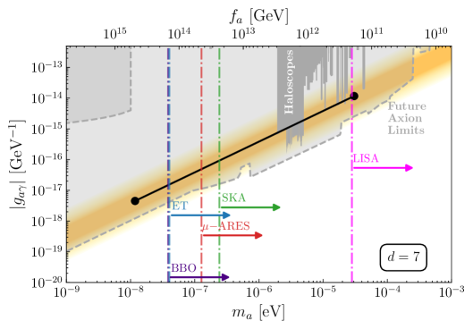
Figure 11: Similar to Fig. 1 but with the possible reaches of future GW detectors. Left panel is for $d=6$ and right panel is $d=7$.

5 Discussion and Conclusion

In this article we have explored the potential to use inflationary GWs to gain information about high-scale QCD axion models. Recent work has shown that many simple QCD axion models generate an early period of heavy quark domination, this has the consequence of increasing the number of viable post-inflationary axion models. Interestingly, the number of model-types which do not have a domain wall problem has now increased from 2 to 8. The non-standard cosmology however alters the misalignment mechanism requiring a larger $f_{a}$ (lower $m_{a}$) to reproduce the correct dark matter abundance.

We have presented an effective model framework to analyse the axion models, focusing on heavy quark decays that proceed through dimension 6 and 7 terms. By varying all relevant parameters, $f_{a},\,m_{Q},$ and $\Lambda$, we show that there is substantial freedom in the mass of the QCD axion dark matter, this has not been pointed out previously. As a consequence, we have found the post-inflationary PQ breaking scenario can easily reproduce similar results than those typically associated with pre-inflationary breaking, i.e. $m_{a}\lesssim 10^{-5}\,{\rm eV}$ and $\Delta N_{\rm eff}\ll 0.027$.

We propose using the stochastic GW background generated from inflation as a way to determine whether a period of HQD occurred. By using such GWs to trace the early epochs of the Universe, we can obtain information on the particle physics that leads to matter domination. To assess the maximum sensitivity these probes will have, we optimistically take a blue-titled GW power spectrum, $n_{T}=0.5$. Such spectra are well motivated by a range of alternatives to the standard single field, slow-roll inflation. A more comprehensive study would allow the parameters that control the GW power spectrum $A_{T}$ and $n_{T}$, to vary, however by setting optimistic but valid values for such parameters we effectively determine the possible reach of future interferometers.

We found that GWs are only sensitive to two parameters in our effective setup, $m_{Q}$ and $\Lambda$, as well as dimension of decay, $d$. In all cases large portions of the particle physics parameter space could be probed in future GW experiments, see Fig. 11. When fixing the QCD axion to be 100% of the dark matter observed we can then fix the decay constant $f_{a}$ allowing us to understand the complementarity between GW probes and axion haloscope experiments. We highlight this in Fig. 11 where we show BBO and ET exhibit the highest potential, capable of probing scenarios where $m_{a}\gtrsim 3\times 10^{-8}$ eV, and $\mu-$ARES can reach $m_{a}>10^{-7}$ eV, for dimension $6$ and $7$ decays. Notably, the difference between dimension $6$ and $7$ decay for probing axion mass is not significantly large.

If the characteristic features of the GW spectral shapes proposed in this study are observed, one may then perform parameter reconstructions for the effective models we investigate. With only the information of the GW spectrum, distinguishing between HQD and other forms of early matter domination may prove challenging. It is only with the additional confirmation from axion haloscope experiments will the HQD explanation look more likely than other forms of early matter domination. At this point, by measuring the strength of $g_{a\gamma}$ one may be able to infer the anomaly coefficients and therefore the corresponding axion models.

On the other hand, in the event of a positive detection of a light QCD axion, no $\Delta N_{\rm eff}$ and no of inflationary GWs, HQD would remain as plausible as pre-inflationary case. This is because our investigation has relied on the blue-tilt of the spectrum. It is true that a slightly red-tilted spectrum may still be detectable in future GW detectore. We believe that further investigations into experimental methods to probe the possibility that HQD occurred in the early Universe are warranted. GAN [26], RADES [197], and QUAX [198]. Experiments using a different technology but probing a similar mass range are MADMAX [199], BABYIAXO [30] and FLASH [29]. For lower axion masses in the $10^{-9}$ to $10^{-7}$ eV range, experiments such as SRF [200, 201], DMRadio [31], and ABRACADABRA [202] show particular promise.

In this paper we have highlighted that the precision era of gravitational wave cosmology holds significant potential for meaningfully probing fundamental physics. We have presented a proof-of-concept whereby the measurement of inflationary gravitational waves could break the experimental deadlock between pre- and post-inflationary PQ breaking scenarios for dark matter axion models.

Appendix A Appendix: Noise modelling for the GW detectors

As already mentioned in Sec. 3.2, estimate of noise spectra associated with the detectors, while assessing the signal. In our study, to asses the signal, we consider the instrumental noise for the aforementioned GW detectors. For LISA and BBO, noise spectra is estimated in terms of effective noise power spectral density ($S(f)$), which can be related with the noise spectra of the detectors as [203]:

$$\Omega_{\rm GW}^{\rm noise}(f)\;=\;\left(\frac{4\pi^{2}}{3H_{0}^{2}}\right)f^{3}S(f).$$ (A.1)

• LISA: Instrumental noise of LISA has two key sources: acceleration noise of test mass (acc) and optical metrology noise (omn) [203]. In terms of power spectral density, instrumental noise is expressed as [204]:

  $$S_{\rm acc}(f) =9\times 10^{-30}\frac{1}{(2\pi f/1{\rm Hz})^{4}}\left(1+\frac{10^{-4}}{f/1{\rm Hz}}\right)~{\rm m^{2}Hz^{-1}},$$ (A.2)

  $$S_{\rm oms}(f) =\left(1.5\times 10^{-11}{\rm m}\right)^{2}\left[1+\left(\frac{2{\rm mHz}}{f}\right)^{4}\right]\,{\rm Hz}^{-1}.$$ (A.3)

  Thus, we have for LISA

  $$S_{\rm LISA}(f) =\frac{10}{3L^{2}}\left(2S_{\rm acc}(f)\left(1+{\rm cos}^{2}\left(\frac{f}{c/(2\pi L)}\right)\right)+S_{\rm oms}(f)\right)\left[1+\frac{6}{10}\left(\frac{f}{c/(2\pi L)}\right)^{2}\right],$$ (A.4)

  where $L=2.5\times 10^{9}$ m is the arm-length of LISA. Thus, using Eq. (A.1), the GW energy density power spectrum can be calculated.

• BBO: For BBO, the non sky-averaged instrumental noise power spectral density is [168]

  $$S_{\rm BBO}(f) =\left[1.8\times 10^{-49}(f/1{\rm Hz})^{2}+2.9\times 10^{-49}+9.2\times 10^{-52}(f/1{\rm Hz})^{-4}\right]~{\rm Hz^{-1}}.$$ (A.5)

  Hence, using Eq. (A.1), $\Omega_{\rm GW}^{\rm noise}$ for BBO can be calculated.

For ET and SKA, we have followed Ref. [205] to generate the noise spectra. The characteristic strain of noise ($h_{c}^{\rm noise}$) for the instrumentation of $\mathbf{\mu}$-ARES is provided in Ref. [176]. The noise spectra can be calculated using $h_{c}$ as [132]

$$h_{c}^{\rm noise}(f)\simeq 1.26\times^{-18}\left(\frac{1\,{\rm Hz}}{f}\right)\sqrt{h^{2}\Omega^{\rm noise}_{\rm GW}(f)}.$$ (A.6)

References

- [1] R.D. Peccei and H.R. Quinn, CP Conservation in the Presence of Instantons, Phys. Rev. Lett. 38 (1977) 1440.
- [2] R.D. Peccei and H.R. Quinn, Some Aspects of Instantons, Nuovo Cim. A 41 (1977) 309.
- [3] S. Weinberg, A New Light Boson?, Phys. Rev. Lett. 40 (1978) 223.
- [4] F. Wilczek, Problem of Strong and Invariance in the Presence of Instantons, Phys. Rev. Lett. 40 (1978) 279.
- [5] J. Preskill, M.B. Wise and F. Wilczek, Cosmology of the Invisible Axion, Phys. Lett. B 120 (1983) 127.
- [6] M. Dine and W. Fischler, The Not So Harmless Axion, Phys. Lett. B 120 (1983) 137.
- [7] L.F. Abbott and P. Sikivie, A Cosmological Bound on the Invisible Axion, Phys. Lett. B 120 (1983) 133.
- [8] P. Sikivie, Axion Cosmology, Lect. Notes Phys. 741 (2008) 19 [astro-ph/0610440].
- [9] D.J.E. Marsh, Axion Cosmology, Phys. Rept. 643 (2016) 1 [1510.07633].
- [10] M. Cirelli, A. Strumia and J. Zupan, Dark Matter, 2406.01705.
- [11] P. Carenza, T. Fischer, M. Giannotti, G. Guo, G. Martínez-Pinedo and A. Mirizzi, Improved axion emissivity from a supernova via nucleon-nucleon bremsstrahlung, JCAP 10 (2019) 016 [1906.11844].
- [12] NA62 collaboration, The Beam and detector of the NA62 experiment at CERN, JINST 12 (2017) P05025 [1703.08501].
- [13] KOTO collaboration, The J-PARC KOTO experiment, PTEP 2012 (2012) 02B006.
- [14] J. Martin Camalich, M. Pospelov, P.N.H. Vuong, R. Ziegler and J. Zupan, Quark Flavor Phenomenology of the QCD Axion, Phys. Rev. D 102 (2020) 015023 [2002.04623].
- [15] G. Alonso-Álvarez, J.M. Cline and T. Xiao, The flavor of QCD axion dark matter, JHEP 07 (2023) 187 [2305.00018].
- [16] ADMX collaboration, A SQUID-based microwave cavity search for dark-matter axions, Phys. Rev. Lett. 104 (2010) 041301 [0910.5914].
- [17] ADMX collaboration, Extended Search for the Invisible Axion with the Axion Dark Matter Experiment, Phys. Rev. Lett. 124 (2020) 101303 [1910.08638].
- [18] Y. Kim et al., Experimental Search for Invisible Dark Matter Axions around 22 eV, Phys. Rev. Lett. 133 (2024) 051802 [2312.11003].
- [19] C. Hagmann et al., First results from a second generation galactic axion experiment, Nucl. Phys. B Proc. Suppl. 51 (1996) 209 [astro-ph/9607022].
- [20] TASEH collaboration, First Results from the Taiwan Axion Search Experiment with a Haloscope at 19.6 eV, Phys. Rev. Lett. 129 (2022) 111802 [2205.05574].
- [21] HAYSTAC collaboration, Results from phase 1 of the HAYSTAC microwave cavity axion experiment, Phys. Rev. D 97 (2018) 092001 [1803.03690].
- [22] QUAX collaboration, Search for galactic axions with a traveling wave parametric amplifier, Phys. Rev. D 108 (2023) 062005 [2304.07505].
- [23] QUAX collaboration, Search for axion dark matter with the QUAX–LNF tunable haloscope, Phys. Rev. D 110 (2024) 022008 [2402.19063].
- [24] P. Brun, A. Caldwell, L. Chevalier, G. Dvali, P. Freire, E. Garutti et al., A new experimental approach to probe QCD axion dark matter in the mass range above { 40} { }{eV}, European Physical Journal C 79 (2019) 186 [1901.07401].
- [25] J. Egge, D. Leppla-Weber, S. Knirck, B. Ary dos Santos Garcia, D. Bergermann, A. Caldwell et al., First search for dark photon dark matter with a MADMAX prototype, arXiv e-prints (2024) arXiv:2408.02368 [2408.02368].
- [26] B.T. McAllister, G. Flower, J. Kruger, E.N. Ivanov, M. Goryachev, J. Bourhill et al., The ORGAN Experiment: An axion haloscope above 15 GHz, Phys. Dark Univ. 18 (2017) 67 [1706.00209].
- [27] B.T. McAllister and M.E. Tobar, The organ experiment, in Microwave Cavities and Detectors for Axion Research, G. Carosi and G. Rybka, eds., (Cham), pp. 37–43, Springer International Publishing, 2020.
- [28] D. Alesini, D. Babusci, D. Di Gioacchino, C. Gatti, G. Lamanna and C. Ligi, The KLASH Proposal, 1707.06010.
- [29] D. Alesini et al., The future search for low-frequency axions and new physics with the FLASH resonant cavity experiment at Frascati National Laboratories, Phys. Dark Univ. 42 (2023) 101370 [2309.00351].
- [30] S. Ahyoune et al., A Proposal for a Low-Frequency Axion Search in the 1–2 eV Range and Below with the BabyIAXO Magnet, Annalen Phys. 535 (2023) 2300326 [2306.17243].
- [31] DMRadio collaboration, Projected sensitivity of DMRadio-m3: A search for the QCD axion below 1 eV, Phys. Rev. D 106 (2022) 103008 [2204.13781].
- [32] R. Allahverdi et al., The First Three Seconds: a Review of Possible Expansion Histories of the Early Universe, 2006.16182.
- [33] Y.B. Zeldovich, I.Y. Kobzarev and L.B. Okun, Cosmological Consequences of the Spontaneous Breakdown of Discrete Symmetry, Zh. Eksp. Teor. Fiz. 67 (1974) 3.
- [34] P. Sikivie, Of Axions, Domain Walls and the Early Universe, Phys. Rev. Lett. 48 (1982) 1156.
- [35] S.M. Barr and J.E. Kim, New Confining Force Solution of the QCD Axion Domain-Wall Problem, Phys. Rev. Lett. 113 (2014) 241301 [1407.4311].
- [36] M. Reig, On the high-scale instanton interference effect: axion models without domain wall problem, JHEP 08 (2019) 167 [1901.00203].
- [37] A. Caputo and M. Reig, Cosmic implications of a low-scale solution to the axion domain wall problem, Phys. Rev. D 100 (2019) 063530 [1905.13116].
- [38] L. Di Luzio, F. Mescia and E. Nardi, Redefining the Axion Window, Phys. Rev. Lett. 118 (2017) 031801 [1610.07593].
- [39] L. Di Luzio, F. Mescia and E. Nardi, Window for preferred axion models, Phys. Rev. D 96 (2017) 075003 [1705.05370].
- [40] A. Cheek, J.K. Osiński and L. Roszkowski, Extending preferred axion models via heavy-quark induced early matter domination, JCAP 03 (2024) 061 [2310.16087].
- [41] L. Di Luzio, S. Hoof, C. Marinissen and V. Plakkot, Catalogues of Cosmologically Self-Consistent Hadronic QCD Axion Models, 2412.17896.
- [42] L.P. Grishchuk, Amplification of gravitational waves in an istropic universe, Zh. Eksp. Teor. Fiz. 67 (1974) 825.
- [43] A.A. Starobinsky, Spectrum of relict gravitational radiation and the early state of the universe, JETP Lett. 30 (1979) 682.
- [44] V.A. Rubakov, M.V. Sazhin and A.V. Veryaskin, Graviton Creation in the Inflationary Universe and the Grand Unification Scale, Phys. Lett. B 115 (1982) 189.
- [45] M.C. Guzzetti, N. Bartolo, M. Liguori and S. Matarrese, Gravitational waves from inflation, Riv. Nuovo Cim. 39 (2016) 399 [1605.01615].
- [46] N. Seto and J. Yokoyama, Probing the equation of state of the early universe with a space laser interferometer, J. Phys. Soc. Jap. 72 (2003) 3082 [gr-qc/0305096].
- [47] L.A. Boyle and P.J. Steinhardt, Probing the early universe with inflationary gravitational waves, Phys. Rev. D 77 (2008) 063504 [astro-ph/0512014].
- [48] L.A. Boyle and A. Buonanno, Relating gravitational wave constraints from primordial nucleosynthesis, pulsar timing, laser interferometers, and the CMB: Implications for the early Universe, Phys. Rev. D 78 (2008) 043531 [0708.2279].
- [49] S. Kuroyanagi, T. Chiba and N. Sugiyama, Precision calculations of the gravitational wave background spectrum from inflation, Phys. Rev. D 79 (2009) 103501 [0804.3249].
- [50] K. Nakayama and J. Yokoyama, Gravitational Wave Background and Non-Gaussianity as a Probe of the Curvaton Scenario, JCAP 01 (2010) 010 [0910.0715].
- [51] S. Kuroyanagi, C. Ringeval and T. Takahashi, Early universe tomography with CMB and gravitational waves, Phys. Rev. D 87 (2013) 083502 [1301.1778].
- [52] R. Jinno, T. Moroi and K. Nakayama, Inflationary Gravitational Waves and the Evolution of the Early Universe, JCAP 01 (2014) 040 [1307.3010].
- [53] K. Saikawa and S. Shirai, Primordial gravitational waves, precisely: The role of thermodynamics in the Standard Model, JCAP 05 (2018) 035 [1803.01038].
- [54] C. Chen, K. Dimopoulos, C. Eröncel and A. Ghoshal, Enhanced primordial gravitational waves from a stiff postinflationary era due to an oscillating inflaton, Phys. Rev. D 110 (2024) 063554 [2405.01679].
- [55] A. Ghoshal, D. Paul and S. Pal, Primordial gravitational waves as probe of dark matter in interferometer missions: Fisher forecast and MCMC, JHEP 12 (2024) 150 [2405.06741].
- [56] M.R. Haque, D. Maity, T. Paul and L. Sriramkumar, Decoding the phases of early and late time reheating through imprints on primordial gravitational waves, Physical Review D 104 (2021) .
- [57] A. Chakraborty, M.R. Haque, D. Maity and R. Mondal, Inflaton phenomenology via reheating in light of primordial gravitational waves and the latest BICEP/Keck data, Phys. Rev. D 108 (2023) 023515 [2304.13637].
- [58] S. Maity and M.R. Haque, Probing the early universe with future GW observatories, 2407.18246.
- [59] M. Berbig and A. Ghoshal, Impact of high-scale Seesaw and Leptogenesis on inflationary tensor perturbations as detectable gravitational waves, JHEP 05 (2023) 172 [2301.05672].
- [60] Z.A. Borboruah, A. Ghoshal, L. Malhotra and U. Yajnik, Inflationary Gravitational Wave Spectral Shapes as test for Low-Scale Leptogenesis, 2405.06603.
- [61] Z.A. Borboruah, A. Ghoshal and S. Ipek, Probing flavor violation and baryogenesis via primordial gravitational waves, JHEP 07 (2024) 228 [2405.03241].
- [62] N. Bernal, A. Ghoshal, F. Hajkarim and G. Lambiase, Primordial Gravitational Wave Signals in Modified Cosmologies, JCAP 11 (2020) 051 [2008.04959].
- [63] S. Datta and R. Samanta, Gravitational waves-tomography of Low-Scale-Leptogenesis, JHEP 11 (2022) 159 [2208.09949].
- [64] S. Datta and R. Samanta, Fingerprints of GeV scale right-handed neutrinos on inflationary gravitational waves and PTA data, Phys. Rev. D 108 (2023) L091706 [2307.00646].
- [65] M. Chianese, S. Datta, R. Samanta and N. Saviano, Tomography of flavoured leptogenesis with primordial blue gravitational waves, JCAP 11 (2024) 051 [2405.00641].
- [66] Z.A. Borboruah, L. Malhotra, F.F. Deppisch and A. Ghoshal, Inflationary Gravitational Waves and Laboratory Searches as Complementary Probes of Right-handed Neutrinos, 2504.15374.
- [67] A.R. Zhitnitsky, On Possible Suppression of the Axion Hadron Interactions. (In Russian), Sov. J. Nucl. Phys. 31 (1980) 260.
- [68] M. Dine, W. Fischler and M. Srednicki, A Simple Solution to the Strong CP Problem with a Harmless Axion, Phys. Lett. B 104 (1981) 199.
- [69] J.E. Kim and G. Carosi, Axions and the Strong CP Problem, Rev. Mod. Phys. 82 (2010) 557 [0807.3125].
- [70] J.E. Kim, Weak Interaction Singlet and Strong CP Invariance, Phys. Rev. Lett. 43 (1979) 103.
- [71] M.A. Shifman, A.I. Vainshtein and V.I. Zakharov, Can Confinement Ensure Natural CP Invariance of Strong Interactions?, Nucl. Phys. B 166 (1980) 493.
- [72] L. Di Luzio, M. Giannotti, E. Nardi and L. Visinelli, The landscape of QCD axion models, Phys. Rept. 870 (2020) 1 [2003.01100].
- [73] G. Grilli di Cortona, E. Hardy, J. Pardo Vega and G. Villadoro, The QCD axion, precisely, JHEP 01 (2016) 034 [1511.02867].
- [74] P.J. Steinhardt and M.S. Turner, Saving the Invisible Axion, Phys. Lett. B 129 (1983) 51.
- [75] G. Lazarides, R.K. Schaefer, D. Seckel and Q. Shafi, Dilution of Cosmological Axions by Entropy Production, Nucl. Phys. B 346 (1990) 193.
- [76] M. Kawasaki, T. Moroi and T. Yanagida, Can decaying particles raise the upper bound on the Peccei-Quinn scale?, Phys. Lett. B 383 (1996) 313 [hep-ph/9510461].
- [77] L. Visinelli and P. Gondolo, Axion cold dark matter in non-standard cosmologies, Phys. Rev. D 81 (2010) 063508 [0912.0015].
- [78] A.E. Nelson and H. Xiao, Axion Cosmology with Early Matter Domination, Phys. Rev. D 98 (2018) 063516 [1807.07176].
- [79] N. Ramberg and L. Visinelli, Probing the Early Universe with Axion Physics and Gravitational Waves, Phys. Rev. D 99 (2019) 123513 [1904.05707].
- [80] P. Arias, N. Bernal, D. Karamitros, C. Maldonado, L. Roszkowski and M. Venegas, New opportunities for axion dark matter searches in nonstandard cosmological models, JCAP 11 (2021) 003 [2107.13588].
- [81] Y. Xu, Constraining axion and ALP dark matter from misalignment during reheating, Phys. Rev. D 108 (2023) 083536 [2308.15322].
- [82] P. Arias, N. Bernal, J.K. Osiński and L. Roszkowski, Dark matter axions in the early universe with a period of increasing temperature, JCAP 05 (2023) 028 [2207.07677].
- [83] P. Arias, N. Bernal, J.K. Osiński, L. Roszkowski and M. Venegas, Revisiting signatures of thermal axions in nonstandard cosmologies, Phys. Rev. D 109 (2024) 123529 [2308.01352].
- [84] M. Kawasaki, K. Kohri and T. Moroi, Big-Bang nucleosynthesis and hadronic decay of long-lived massive particles, Phys. Rev. D 71 (2005) 083502 [astro-ph/0408426].
- [85] K. Jedamzik, Big bang nucleosynthesis constraints on hadronically and electromagnetically decaying relic neutral particles, Phys. Rev. D 74 (2006) 103509 [hep-ph/0604251].
- [86] K. Jedamzik, Bounds on long-lived charged massive particles from Big Bang nucleosynthesis, JCAP 03 (2008) 008 [0710.5153].
- [87] M. Kawasaki, K. Kohri, T. Moroi and Y. Takaesu, Revisiting Big-Bang Nucleosynthesis Constraints on Long-Lived Decaying Particles, Phys. Rev. D 97 (2018) 023502 [1709.01211].
- [88] C. Chen, S. Jyoti Das, K. Dimopoulos and A. Ghoshal, Flipped Rotating Axion Non-minimally Coupled to Gravity: Baryogenesis and Dark Matter, 2502.08720.
- [89] A. Cheek and U. Min, Using N eff to constrain preferred axion model dark matter, JCAP 03 (2025) 014 [2411.17320].
- [90] D. Karamitros, MiMeS: Misalignment mechanism solver, Comput. Phys. Commun. 275 (2022) 108311 [2110.12253].
- [91] S. Borsanyi et al., Calculation of the axion mass based on high-temperature lattice quantum chromodynamics, Nature 539 (2016) 69 [1606.07494].
- [92] Planck collaboration, Planck 2018 results. VI. Cosmological parameters, Astron. Astrophys. 641 (2020) A6 [1807.06209].
- [93] C. O’Hare, “cajohare/axionlimits: Axionlimits.” https://cajohare.github.io/AxionLimits/, July, 2020. 10.5281/zenodo.3932430.
- [94] I. Stern, ADMX Status, PoS ICHEP2016 (2016) 198 [1612.08296].
- [95] CAPP collaboration, First Results from an Axion Haloscope at CAPP around 10.7 eV, Phys. Rev. Lett. 126 (2021) 191802 [2012.10764].
- [96] B. Yang, H. Yoon, M. Ahn, Y. Lee and J. Yoo, Extended Axion Dark Matter Search Using the CAPP18T Haloscope, Phys. Rev. Lett. 131 (2023) 081801 [2308.09077].
- [97] CAPP collaboration, Extensive Search for Axion Dark Matter over 1 GHz with CAPP’S Main Axion Experiment, Phys. Rev. X 14 (2024) 031023 [2402.12892].
- [98] T.W.B. Kibble, Topology of Cosmic Domains and Strings, J. Phys. A 9 (1976) 1387.
- [99] T.W.B. Kibble, G. Lazarides and Q. Shafi, Walls Bounded by Strings, Phys. Rev. D 26 (1982) 435.
- [100] A. Vilenkin and A.E. Everett, Cosmic Strings and Domain Walls in Models with Goldstone and PseudoGoldstone Bosons, Phys. Rev. Lett. 48 (1982) 1867.
- [101] C. Hagmann, S. Chang and P. Sikivie, Axion radiation from strings, Phys. Rev. D 63 (2001) 125018 [hep-ph/0012361].
- [102] O. Wantz and E.P.S. Shellard, Axion Cosmology Revisited, Phys. Rev. D 82 (2010) 123508 [0910.1066].
- [103] T. Hiramatsu, M. Kawasaki, T. Sekiguchi, M. Yamaguchi and J. Yokoyama, Improved estimation of radiated axions from cosmological axionic strings, Phys. Rev. D 83 (2011) 123531 [1012.5502].
- [104] M. Kawasaki, K. Saikawa and T. Sekiguchi, Axion dark matter from topological defects, Phys. Rev. D 91 (2015) 065014 [1412.0789].
- [105] M. Buschmann, J.W. Foster, A. Hook, A. Peterson, D.E. Willcox, W. Zhang et al., Dark matter from axion strings with adaptive mesh refinement, Nature Commun. 13 (2022) 1049 [2108.05368].
- [106] M. Gorghetto, E. Hardy and H. Nicolaescu, Observing invisible axions with gravitational waves, JCAP 06 (2021) 034 [2101.11007].
- [107] H. Kim, J. Park and M. Son, Axion dark matter from cosmic string network, JHEP 07 (2024) 150 [2402.00741].
- [108] P.D. Meerburg, R. Hložek, B. Hadzhiyska and J. Meyers, Multiwavelength constraints on the inflationary consistency relation, Phys. Rev. D 91 (2015) 103505 [1502.00302].
- [109] A.R. Liddle and D.H. Lyth, Inflation and mixed dark matter models, Mon. Not. Roy. Astron. Soc. 265 (1993) 379 [astro-ph/9304017].
- [110] LIGO Scientific, Virgo collaboration, Upper Limits on the Stochastic Gravitational-Wave Background from Advanced LIGO’s First Observing Run, Phys. Rev. Lett. 118 (2017) 121101 [1612.02029].
- [111] LIGO Scientific collaboration, Searching for a Stochastic Background of Gravitational Waves with LIGO, Astrophys. J. 659 (2007) 918 [astro-ph/0608606].
- [112] G. Cabass, L. Pagano, L. Salvati, M. Gerbino, E. Giusarma and A. Melchiorri, Updated Constraints and Forecasts on Primordial Tensor Modes, Phys. Rev. D 93 (2016) 063508 [1511.05146].
- [113] B. Allen and J.D. Romano, Detecting a stochastic background of gravitational radiation: Signal processing strategies and sensitivities, Phys. Rev. D 59 (1999) 102001 [gr-qc/9710117].
- [114] LIGO Scientific, VIRGO collaboration, Upper limits on a stochastic gravitational-wave background using LIGO and Virgo interferometers at 600-1000 Hz, Phys. Rev. D 85 (2012) 122001 [1112.5004].
- [115] A.R. Liddle and D.H. Lyth, The Cold dark matter density perturbation, Phys. Rept. 231 (1993) 1 [astro-ph/9303019].
- [116] R.H. Brandenberger, A. Nayeri, S.P. Patil and C. Vafa, Tensor Modes from a Primordial Hagedorn Phase of String Cosmology, Phys. Rev. Lett. 98 (2007) 231302 [hep-th/0604126].
- [117] G. Calcagni, S. Kuroyanagi, J. Ohashi and S. Tsujikawa, Strong Planck constraints on braneworld and non-commutative inflation, JCAP 03 (2014) 052 [1310.5186].
- [118] T. Fujita, S. Kuroyanagi, S. Mizuno and S. Mukohyama, Blue-tilted Primordial Gravitational Waves from Massive Gravity, Phys. Lett. B 789 (2019) 215 [1808.02381].
- [119] J.L. Cook and L. Sorbo, Particle production during inflation and gravitational waves detectable by ground-based interferometers, Phys. Rev. D 85 (2012) 023534 [1109.0022].
- [120] S. Mukohyama, R. Namba, M. Peloso and G. Shiu, Blue Tensor Spectrum from Particle Production during Inflation, JCAP 08 (2014) 036 [1405.0346].
- [121] T. Kobayashi, M. Yamaguchi and J. Yokoyama, G-inflation: Inflation driven by the Galileon field, Phys. Rev. Lett. 105 (2010) 231302 [1008.0603].
- [122] P. Adshead, E. Martinec, E.I. Sfakianakis and M. Wyman, Higgsed Chromo-Natural Inflation, JHEP 12 (2016) 137 [1609.04025].
- [123] M.M. Anber and L. Sorbo, Naturally inflating on steep potentials through electromagnetic dissipation, Phys. Rev. D 81 (2010) 043534 [0908.4089].
- [124] M. Baldi, F. Finelli and S. Matarrese, Inflation with violation of the null energy condition, Phys. Rev. D 72 (2005) 083504 [astro-ph/0505552].
- [125] V.K. Oikonomou, A refined Einstein–Gauss–Bonnet inflationary theoretical framework, Class. Quant. Grav. 38 (2021) 195025 [2108.10460].
- [126] M. Biagetti, M. Fasiello and A. Riotto, Enhancing Inflationary Tensor Modes through Spectator Fields, Phys. Rev. D 88 (2013) 103518 [1305.7241].
- [127] R.R. Caldwell and C. Devulder, Axion Gauge Field Inflation and Gravitational Leptogenesis: A Lower Bound on B Modes from the Matter-Antimatter Asymmetry of the Universe, Phys. Rev. D 97 (2018) 023532 [1706.03765].
- [128] E. Dimastrogiovanni, M. Fasiello, R.J. Hardwick, H. Assadullahi, K. Koyama and D. Wands, Non-Gaussianity from Axion-Gauge Fields Interactions during Inflation, JCAP 11 (2018) 029 [1806.05474].
- [129] P. Adshead and E.I. Sfakianakis, Higgsed Gauge-flation, JHEP 08 (2017) 130 [1705.03024].
- [130] S. Kuroyanagi, T. Takahashi and S. Yokoyama, Blue-tilted inflationary tensor spectrum and reheating in the light of NANOGrav results, JCAP 01 (2021) 071 [2011.03323].
- [131] NANOGrav collaboration, The NANOGrav 15 yr Data Set: Search for Signals from New Physics, Astrophys. J. Lett. 951 (2023) L11 [2306.16219].
- [132] M. Maggiore, Gravitational wave experiments and early universe cosmology, Phys. Rept. 331 (2000) 283 [gr-qc/9909001].
- [133] R.H. Cyburt, B.D. Fields, K.A. Olive and T.-H. Yeh, Big Bang Nucleosynthesis: 2015, Rev. Mod. Phys. 88 (2016) 015004 [1505.01076].
- [134] CMB Bharat Collaboration collaboration, CMB Bharat, .
- [135] K. Abazajian et al., CMB-S4 Science Case, Reference Design, and Project Plan, 1907.04473.
- [136] Topical Conveners: K.N. Abazajian, J.E. Carlstrom, A.T. Lee collaboration, Neutrino Physics from the Cosmic Microwave Background and Large Scale Structure, Astropart. Phys. 63 (2015) 66 [1309.5383].
- [137] NASA PICO collaboration, PICO: Probe of Inflation and Cosmic Origins, 1902.10541.
- [138] CMB-HD collaboration, Snowmass2021 CMB-HD White Paper, 2203.05728.
- [139] CORE collaboration, Exploring cosmic origins with CORE: Survey requirements and mission design, JCAP 04 (2018) 014 [1706.04516].
- [140] SPT-3G collaboration, SPT-3G: A Next-Generation Cosmic Microwave Background Polarization Experiment on the South Pole Telescope, Proc. SPIE Int. Soc. Opt. Eng. 9153 (2014) 91531P [1407.2973].
- [141] Simons Observatory collaboration, The Simons Observatory: Science goals and forecasts, JCAP 02 (2019) 056 [1808.07445].
- [142] M.S. Turner, M.J. White and J.E. Lidsey, Tensor perturbations in inflationary models as a probe of cosmology, Phys. Rev. D 48 (1993) 4613 [astro-ph/9306029].
- [143] S. Chongchitnan and G. Efstathiou, Prospects for direct detection of primordial gravitational waves, Phys. Rev. D 73 (2006) 083511 [astro-ph/0602594].
- [144] K. Nakayama, S. Saito, Y. Suwa and J. Yokoyama, Probing reheating temperature of the universe with gravitational wave background, JCAP 06 (2008) 020 [0804.1827].
- [145] S. Kuroyanagi, K. Nakayama and S. Saito, Prospects for determination of thermal history after inflation with future gravitational wave detectors, Phys. Rev. D 84 (2011) 123513 [1110.4169].
- [146] S. Kuroyanagi, T. Takahashi and S. Yokoyama, Blue-tilted Tensor Spectrum and Thermal History of the Universe, JCAP 02 (2015) 003 [1407.4785].
- [147] LIGO Scientific, Virgo collaboration, Observation of Gravitational Waves from a Binary Black Hole Merger, Phys. Rev. Lett. 116 (2016) 061102 [1602.03837].
- [148] LIGO Scientific, Virgo collaboration, GW151226: Observation of Gravitational Waves from a 22-Solar-Mass Binary Black Hole Coalescence, Phys. Rev. Lett. 116 (2016) 241103 [1606.04855].
- [149] LIGO Scientific, VIRGO collaboration, GW170104: Observation of a 50-Solar-Mass Binary Black Hole Coalescence at Redshift 0.2, Phys. Rev. Lett. 118 (2017) 221101 [1706.01812].
- [150] LIGO Scientific, Virgo collaboration, GW170608: Observation of a 19-solar-mass Binary Black Hole Coalescence, Astrophys. J. Lett. 851 (2017) L35 [1711.05578].
- [151] F.A.e.a. M. Punturo, M. Abernathy, The einstein telescope: a third-generation gravitational wave observatory, Classical and Quantum Gravity 27 (2010) 194002.
- [152] S. Hild et al., Sensitivity Studies for Third-Generation Gravitational Wave Observatories, Class. Quant. Grav. 28 (2011) 094013 [1012.0908].
- [153] LIGO Scientific collaboration, Advanced LIGO, Class. Quant. Grav. 32 (2015) 074001 [1411.4547].
- [154] LIGO Scientific, Virgo collaboration, Open data from the first and second observing runs of Advanced LIGO and Advanced Virgo, SoftwareX 13 (2021) 100658 [1912.11716].
- [155] B. Iyer et al., Ligo-india technical report, Tech. Rep. M1100296-v2, LIGO (2011).
- [156] T. Souradeep, S. Raja, Z. Khan, C. Unnikrishnan and B. Iyer, Ligo-india - a unique adventure in indian science, Current Science 113 (2017) 672.
- [157] C.S. Unnikrishnan, IndIGO and LIGO-India: Scope and plans for gravitational wave research and precision metrology in India, Int. J. Mod. Phys. D 22 (2013) 1341010 [1510.06059].
- [158] B.S. Sathyaprakash et al., Scientific benefits of moving one of ligo hanford detectors to india, Tech. Rep. T1200219-v1, LIGO (2012).
- [159] C.S. Unnikrishnan, LIGO-India: A decadal assessment on its scope, relevance, progress and future, Int. J. Mod. Phys. D 33 (2024) 2450025 [2301.07522].
- [160] LIGO Scientific, VIRGO collaboration, All-sky search for gravitational-wave bursts in the first joint LIGO-GEO-Virgo run, Phys. Rev. D 81 (2010) 102001 [1002.1036].
- [161] T. Accadia and et al, Virgo: a laser interferometer to detect gravitational waves, Journal of Instrumentation 7 (2012) 3012.
- [162] LIGO Scientific, Virgo collaboration, GW170814: A Three-Detector Observation of Gravitational Waves from a Binary Black Hole Coalescence, Phys. Rev. Lett. 119 (2017) 141101 [1709.09660].
- [163] LIGO Scientific, Virgo collaboration, GW170817: Observation of Gravitational Waves from a Binary Neutron Star Inspiral, Phys. Rev. Lett. 119 (2017) 161101 [1710.05832].
- [164] Virgo Collaboration collaboration, Increasing the astrophysical reach of the advanced virgo detector via the application of squeezed vacuum states of light, Phys. Rev. Lett. 123 (2019) 231108.
- [165] VIRGO collaboration, Advanced Virgo: a second-generation interferometric gravitational wave detector, Class. Quant. Grav. 32 (2015) 024001 [1408.3978].
- [166] KAGRA collaboration, KAGRA: 2.5 Generation Interferometric Gravitational Wave Detector, Nature Astron. 3 (2019) 35 [1811.08079].
- [167] D. Reitze et al., Cosmic Explorer: The U.S. Contribution to Gravitational-Wave Astronomy beyond LIGO, Bull. Am. Astron. Soc. 51 (2019) 035 [1907.04833].
- [168] K. Yagi, N. Tanahashi and T. Tanaka, Probing the size of extra dimension with gravitational wave astronomy, Phys. Rev. D 83 (2011) 084036 [1101.4997].
- [169] N. Seto, S. Kawamura and T. Nakamura, Possibility of direct measurement of the acceleration of the universe using 0.1-Hz band laser interferometer gravitational wave antenna in space, Phys. Rev. Lett. 87 (2001) 221103 [astro-ph/0108011].
- [170] S. Kawamura, T. Nakamura and M.A. et al., The japanese space gravitational wave antenna—decigo, Classical and Quantum Gravity 23 (2006) S125.
- [171] K. Yagi and N. Seto, Detector configuration of DECIGO/BBO and identification of cosmological neutron-star binaries, Phys. Rev. D 83 (2011) 044011 [1101.3940].
- [172] V. Corbin and N.J. Cornish, Detecting the cosmic gravitational wave background with the big bang observer, Class. Quant. Grav. 23 (2006) 2435 [gr-qc/0512039].
- [173] G.M. Harry, P. Fritschel, D.A. Shaddock, W. Folkner and E.S. Phinney, Laser interferometry for the big bang observer, Classical and Quantum Gravity 23 (2006) 4887.
- [174] P. Amaro-Seoane, H. Audley and S.B. et al., Laser interferometer space antenna, 2017.
- [175] J. Baker et al., The Laser Interferometer Space Antenna: Unveiling the Millihertz Gravitational Wave Sky, 1907.06482.
- [176] A. Sesana et al., Unveiling the gravitational universe at -Hz frequencies, Exper. Astron. 51 (2021) 1333 [1908.11391].
- [177] C.L. Carilli and S. Rawlings, Science with the Square Kilometer Array: Motivation, key science projects, standards and assumptions, New Astron. Rev. 48 (2004) 979 [astro-ph/0409274].
- [178] G. Janssen et al., Gravitational wave astronomy with the SKA, PoS AASKA14 (2015) 037 [1501.00127].
- [179] A. Weltman et al., Fundamental physics with the Square Kilometre Array, Publ. Astron. Soc. Austral. 37 (2020) e002 [1810.02680].
- [180] EPTA collaboration, The European Pulsar Timing Array and the Large European Array for Pulsars, Class. Quant. Grav. 30 (2013) 224009.
- [181] EPTA collaboration, European Pulsar Timing Array Limits On An Isotropic Stochastic Gravitational-Wave Background, Mon. Not. Roy. Astron. Soc. 453 (2015) 2576 [1504.03692].
- [182] EPTA collaboration, European Pulsar Timing Array Limits on Continuous Gravitational Waves from Individual Supermassive Black Hole Binaries, Mon. Not. Roy. Astron. Soc. 455 (2016) 1665 [1509.02165].
- [183] M.A. McLaughlin, The North American Nanohertz Observatory for Gravitational Waves, Class. Quant. Grav. 30 (2013) 224008 [1310.0758].
- [184] NANOGRAV collaboration, The NANOGrav 11-year Data Set: Pulsar-timing Constraints On The Stochastic Gravitational-wave Background, Astrophys. J. 859 (2018) 47 [1801.02617].
- [185] K. Aggarwal et al., The NANOGrav 11-Year Data Set: Limits on Gravitational Waves from Individual Supermassive Black Hole Binaries, Astrophys. J. 880 (2019) 2 [1812.11585].
- [186] A. Brazier et al., The NANOGrav Program for Gravitational Waves and Fundamental Physics, 1908.05356.
- [187] NANOGrav collaboration, The NANOGrav 12.5 yr Data Set: Search for an Isotropic Stochastic Gravitational-wave Background, Astrophys. J. Lett. 905 (2020) L34 [2009.04496].
- [188] BICEP, Keck collaboration, Improved Constraints on Primordial Gravitational Waves using Planck, WMAP, and BICEP/Keck Observations through the 2018 Observing Season, Phys. Rev. Lett. 127 (2021) 151301 [2110.00483].
- [189] BICEP2, Planck collaboration, Joint Analysis of BICEP2/ and Data, Phys. Rev. Lett. 114 (2015) 101301 [1502.00612].
- [190] E. Thrane and J.D. Romano, Sensitivity curves for searches for gravitational-wave backgrounds, Phys. Rev. D 88 (2013) 124032 [1310.5300].
- [191] B. Fu, A. Ghoshal and S.F. King, Cosmic string gravitational waves from global symmetry breaking as a probe of the type I seesaw scale, JHEP 11 (2023) 071 [2306.07334].
- [192] F. Ferrer, E. Masso, G. Panico, O. Pujolas and F. Rompineve, Primordial Black Holes from the QCD axion, Phys. Rev. Lett. 122 (2019) 101301 [1807.01707].
- [193] A. Conaci, L. Delle Rose, P.S.B. Dev and A. Ghoshal, Slaying axion-like particles via gravitational waves and primordial black holes from supercooled phase transition, JHEP 12 (2024) 196 [2401.09411].
- [194] A. Ghoshal, Y. Gouttenoire, L. Heurtier and P. Simakachorn, Primordial black hole archaeology with gravitational waves from cosmic strings, JHEP 08 (2023) 196 [2304.04793].
- [195] S. Datta, A. Ghosal, A. Ghoshal and G. White, Complementarity between Cosmic String Gravitational Waves and long lived particle searches in laboratory, 2501.03326.
- [196] C. Caprini et al., Science with the space-based interferometer eLISA. II: Gravitational waves from cosmological phase transitions, JCAP 04 (2016) 001 [1512.06239].
- [197] A.A. Melcón et al., Axion Searches with Microwave Filters: the RADES project, JCAP 05 (2018) 040 [1803.01243].
- [198] D. Alesini et al., Search for invisible axion dark matter of mass meV with the QUAX– experiment, Phys. Rev. D 103 (2021) 102004 [2012.09498].
- [199] MADMAX collaboration, A new experimental approach to probe QCD axion dark matter in the mass range above 40 eV, Eur. Phys. J. C 79 (2019) 186 [1901.07401].
- [200] A. Berlin, R.T. D’Agnolo, S.A.R. Ellis and K. Zhou, Heterodyne broadband detection of axion dark matter, Phys. Rev. D 104 (2021) L111701 [2007.15656].
- [201] SHANHE collaboration, First Scan Search for Dark Photon Dark Matter with a Tunable Superconducting Radio-Frequency Cavity, Phys. Rev. Lett. 133 (2024) 021005 [2305.09711].
- [202] C.P. Salemi et al., Search for Low-Mass Axion Dark Matter with ABRACADABRA-10 cm, Phys. Rev. Lett. 127 (2021) 081801 [2102.06722].
- [203] C. Gowling and M. Hindmarsh, Observational prospects for phase transitions at LISA: Fisher matrix analysis, JCAP 10 (2021) 039 [2106.05984].
- [204] M. Breitbach, J. Kopp, E. Madge, T. Opferkuch and P. Schwaller, Dark, Cold, and Noisy: Constraining Secluded Hidden Sectors with Gravitational Waves, JCAP 07 (2019) 007 [1811.11175].
- [205] K. Schmitz, New Sensitivity Curves for Gravitational-Wave Signals from Cosmological Phase Transitions, JHEP 01 (2021) 097 [2002.04615].