Active Sampling for MRI-based Sequential Decision Making

Abstract

Despite the superior diagnostic capability of Magnetic Resonance Imaging (MRI), its use as a Point-of-Care (PoC) device remains limited by high cost and complexity. To enable such a future by reducing the magnetic field strength, one key approach will be to improve sampling strategies. Previous work has shown that it is possible to make diagnostic decisions directly from $k$-space with fewer samples. Such work shows that single diagnostic decisions can be made, but if we aspire to see MRI as a true PoC, multiple and sequential decisions are necessary while minimizing the number of samples acquired. We present a novel multi-objective reinforcement learning framework enabling comprehensive, sequential, diagnostic evaluation from undersampled $k$-space data. Our approach during inference actively adapts to sequential decisions to optimally sample. To achieve this, we introduce a training methodology that identifies the samples that contribute the best to each diagnostic objective using a step-wise weighting reward function. We evaluate our approach in two sequential knee pathology assessment tasks: ACL sprain detection and cartilage thickness loss assessment. Our framework achieves diagnostic performance competitive with various policy-based benchmarks on disease detection, severity quantification, and overall sequential diagnosis, while substantially saving $k$-space samples. Our approach paves the way for the future of MRI as a comprehensive and affordable PoC device. Our code is publicly available at https://github.com/vios-s/MRI_Sequential_Active_Sampling.

Computer aided diagnosis, Magnetic resonance imaging, Point of care, Reinforcement learning.

1 Introduction

Despite the proliferation of MRI, its utility as a Point-Of-Care (PoC) diagnostic tool remains limited due to prolonged acquisition times, complex instrumentation, and high cost [1]. A promising solution has emerged through the development of low-field MRI systems [2]. These systems can be deployed at accident sites, in ambulatory settings, or in other areas where immediate decisions are necessary to provide the best treatment options. Thus, such PoC settings are not to replace the utility of MRI as a clinical generic diagnostic tool, but as a bespoke affordable and portable device. However, a reduced magnetic field strength [3] does degrade imaging quality. Therefore, improvements in how and where we sample are considered key for unlocking the future of MRI as PoC.

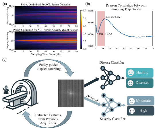
Figure 1: Illustration of our proposed sequential diagnostic framework for active MR acquisition and its motivating evidence: in preliminary experiments, we found similarities between the sampling trajectories of disease detection and severity quantification. We trained policies [4] optimized independently for each task and obtained sampling trajectories shown in (a), and then measured their similarity in (b). We observe an increasing Pearson correlation between sampling steps $4$ and $14$, indicating that in this range $k$-space samples contribute simultaneously to both tasks. These observations motivate our approach (c) to learn a sampling policy that jointly optimizes two tasks, taking into account their sequential nature. During inference, our approach identifies which samples to take using k-space features, considering that one task (severity) will be following the confirmation of the disease.

Recent advances in machine learning methods have allowed a reduction in $k$-space samples and retaining diagnostic utility [5]. A line of work has focused on optimizing sampling trajectories for image reconstruction [6, 7]. More recently, exciting approaches have emerged that aim to drastically reduce sampling by removing redundant information. These methods bypass image reconstruction entirely and make direct inferences from undersampled $k$-space [8, 9].

Decisions even in a PoC setting will be complex and reflect a multilayered decision making process. Hence, high-level decisions (e.g., disease presence) should be made first, followed by additional decisions (e.g., disease severity) to determine subsequent actions (e.g., treatment options). A fundamental research question emerges: Are there correlations in $k$-space patterns between such sequential decisions and can these be exploited for further sampling reductions? If such correlations exist, sampling strategies should be optimized to exploit them. Otherwise, independently optimizing sampling strategies for each diagnostic task leads to sampling inefficiency. Our preliminary experiments (Figure 1) reveal compelling correlation patterns between sampling trajectories.

Leveraging this observation, we develop an AI agent to satisfy both objectives within the same policy, maintaining computational efficiency while structuring binary diagnostics as a structured sequential decision process for comprehensive clinical assessment. To the best of our knowledge, such active sampling strategies for sequential diagnostic tasks have not been previously explored. We reformulate the diagnostic process as a multi-objective reinforcement learning (MORL) sampling optimization problem, sequentially inferring the presence of the disease and its severity in one scanning session.

As illustrated in Figure 1, the core components of our framework include: an RL-based policy network for $k$-space sampling guidance, and dual diagnostic streams for disease detection and severity quantification. The policy network guides data acquisition by leveraging features extracted from accumulated $k$-space measurements, continuously optimizing the sampling trajectory. The diagnostic streams process the undersampled $k$-space hierarchically: the disease classifier performs binary classification to identify diseased subjects, which is followed by severity quantification for positive cases.

Overall, our contributions are summarized as follows:

1. Our research pioneers sequential, dynamic diagnosis from $k$-space data with active sampling, enabling sequential decisions in a single scanning session.

2. A MORL-based policy network employs policy gradient methods with greedy action selection for efficient $k$-space exploration. It optimizes a step-wise weighting reward function to balance disease detection and severity quantification, maximizing diagnostic information gain.

3. Extensive experiments on ACL sprain detection and cartilage thickness loss assessment demonstrate that our method outperforms baselines and benchmarks in diagnostic accuracy, and significantly reduces $k$-space data acquisition time, advancing PoC MRI applications.

2 Related Works

We first review ML-based $k$-space sampling optimization techniques that accelerate acquisition. We then examine direct diagnostic inference approaches from $k$-space, highlighting the research gap in sequential decision making. Finally, we discuss RL-based multi-objective optimization in medical imaging, demonstrating how our sequential sampling framework builds upon these foundations to enable comprehensive diagnosis directly from undersampled $k$-space.

2.1 ML-based $k$-space Sampling Optimization

Accelerating MRI acquisition remains a significant research focus through improved $k$-space undersampling strategies. While the Cartesian grid trajectory predominates in clinical practice due to its robustness [10], conventional undersampling approaches —including equispaced, random, and variable density sampling— prioritize frequency domain characteristics rather than task-specific requirements, potentially compromising clinical accuracy in accelerated acquisitions [11].

Recent works have advanced learning-based sampling methods that optimize diagnostic performance at the population level. These approaches formulate sampling mask optimization either as a probability density function for Cartesian grid selection [6, 12] or as learnable non-Cartesian coordinates[13] in non-uniform Fast Fourier Transform (NUFFT) [14, 15], enabling end-to-end optimization of sampling trajectories and reconstruction performance. While subsequent innovations incorporate generative models [16] and model pruning [17], these methods produce fixed sampling patterns that do not adapt to patient-specific characteristics.

Instead, active sampling strategies adapt to individual patients through sequential $k$-space measurements. Reinforcement learning (RL) has emerged as a powerful framework for this sampling optimization, framing $k$-space sampling as a Markov Decision Process where policies learn to select measurements based on accumulated information. Notable approaches include policy gradient methods with greedy actions [18] and Q-learning [19] for reconstruction optimization. While initial work focused on reconstruction quality, recent studies demonstrate the potential for direct diagnostic inference from undersampled data [20], indicating a paradigm shift from traditional reconstruction-based analysis to efficient, direct $k$-space diagnostic assessment.

2.2 Direct Diagnostic Inference from $k$-space

A new line of work has shown the potential of ‘image-less’ diagnostic processes through direct inference from $k$-space data. This approach reduces the need for reconstruction, saving samples by avoiding redundant and uninformative pixels (voxels). Studies show successful disease classification [4, 8, 9] and segmentation [20] using undersampled $k$-space measurements, without reconstruction. Direct inference with population-level undersampling optimization achieves comparable performance to fully-sampled image analysis, while integration with RL-based active sampling enables patient-level mask optimization and improved classification performance [4, 9]. However, existing approaches primarily optimize sampling for a single objective during a scanning session, leaving multi-objective sampling optimization unexplored. As such any additional redundancy between the sampling patterns for different tasks (and hence different objectives) is unutilized.

2.3 RL-based Multi-objective Optimization in Medical Imaging

Multi-objective optimization in clinical evaluation systems presents a fundamental challenge in medical imaging. While multi-task learning frameworks have been explored extensively [21, 22], the joint optimization of sampling strategies for multiple diagnostic targets remains underexplored. Recent advances in MORL show promising methodological innovations across medical applications [23]. In chest X-ray generation [24], policy-based RL simultaneously optimizes posture alignment, diagnostic conditions, and multimodal consistency through cumulative reward maximization. Similarly, anatomical landmark detection [25] leverages multi-agent frameworks with specialized joint detection while preserving anatomical constraints. Further innovations include consequence-oriented reward functions for simultaneous vertebral detection and segmentation [26], incorporating exponentially weighted attention metrics for balanced task performance.

While various frameworks demonstrate efficacy through weighted rewards [26, 27] and collaborative strategies [25, 28], their application to $k$-space sampling optimization remains unexplored, presenting opportunities for frameworks that simultaneously optimize multiple diagnostic goals.

3 Methodology

3.1 Preliminaries

Instead of directly imaging human anatomy, MRI captures the electromagnetic activity in the body after exposure to magnetic fields and radio-frequency pulses, measured in $k$-space (i.e., the frequency domain). For a single coil measurement, the $k$-space data can be represented as a 2-dimensional complex-valued matrix $\mathbf{x}\in\mathbb{C}^{r\times c}$, where $r$ is the number of rows and $c$ is the number of columns, respectively. The spatial image $\mathbf{I}$ is obtained by applying the inverse Fourier Transform to $\mathbf{x}$, denoted as $\mathbf{I}=\mathcal{F}^{-1}(\mathbf{x})$. The undersampled $k$-space, represented as $\mathbf{x}_{s}$, is modeled by $\mathbf{x}_{s}=U_{L}\circ\mathbf{x}$ where $U_{L}$ can be viewed as a binary mask $U\in\{0,1\}^{r\times c}$ with $L$ measurements sampled in $k$-space. We exclusively consider a Cartesian mask for MRI undersampling. Thus, the undersampled image is denoted as $\mathbf{I}_{s}=\mathcal{F}^{-1}(\mathbf{x}_{s})$.

For clinical diagnosis, radiologists and other clinical experts interpret medical imaging data to first identify the presence of disease ($g_{d}$) and then its severity ($g_{s}$), providing a comprehensive diagnosis. These labels are derived by analyzing the collected $k$-space data after appropriate processing.

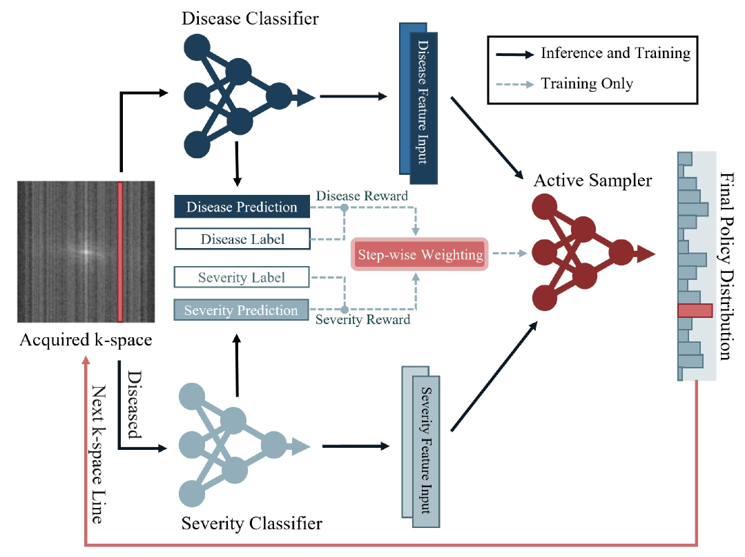
Figure 2: Illustration of the proposed sequential diagnostic active sampling. Initially, a randomly sampled $k$-space subset is fed into two pre-trained disease and severity classifiers. The active sampler takes as input the features extracted by the classifiers and decides the next $k$-space sampling location. After exhausting the sampling budget or meeting a user-defined criterion, the disease classifier confirms the presence of disease and subsequently the severity classifier is queried to estimate the severity level. During training, the active sampler is optimized with a novel step-wise weighting mechanism that combines the disease and severity rewards and enables a smooth transition.

3.2 Framework Workflow

As shown in Figure 2, our framework aims to reduce acquisition time by selectively and progressively sampling the $k$-space, considering sequential diagnostic tasks.

The process begins with a small subset of randomly sampled $k$-space with $L$ measurements, denoted as $\mathbf{x}_{s_{0}}=U_{L}\circ\mathbf{x}$, which is passed to task-specific classifiers. The pre-trained disease and severity classification networks $f_{d}$ and $f_{s}$, generate the initial disease and severity prediction $y_{d_{0}}$ and $y_{s_{0}}$. The high-level feature maps $m_{0}$, from both classifiers are extracted and then fed into the Active Sampler $S$, where the policy network, parameterized by $\phi$, generates a sampling policy $\pi_{\phi}(m_{0})$ to guide the selective sampling of diagnostically significant lines in $k$-space. These sampled lines are subsequently added to $U_{L}$. The updated $k$-space subset at step $t\in[0,T]$ is denoted as $\mathbf{x}_{s_{t}}=U_{t}\circ\mathbf{x}$ and fed back into the classification network. The iterative process continues until the sampling budget $T$ is exhausted or some user-defined reliability criterion (e.g., confidence score) is satisfied. During the training stage, we separately calculate the disease reward $r_{d}=r(y_{d},g_{d})$ and severity reward $r_{s}=r(y_{s},g_{s})$ using classifier predictions and the ground truth labels. An obvious and naive approach would be to directly use the rewards to supervise the active sampler; however, this will not learn the sequential aspect of the two objectives. Instead, we propose here to use a step-wise weighting procedure to shift the emphasis of sampling strategy from one objective to the other as sampling steps progress. In addition, to further enforce the sequential nature (i.e., disease prediction should precede severity), if the disease prediction is ‘No findings’ for a subject, the severity reward will not be applied for supervision.

3.3 Undersampled k-Space Classification Networks

To perform direct prediction with undersampled $k$-space data, we pre-train a disease classifier $f_{d}$ with undersampled data and ground truth label $g_{d}$. For the severity classifier $f_{s}$, we fine-tune the disease classifier with only diseased data and the associated severity labels $g_{s}$. For severity quantification, fine-tuning prevents potential overfitting caused by data scarcity and reuses the knowledge learned by the disease classifier. These pre-trained classifiers act as the reward model in the training process of the active sampler. They also function as a feature extractor, providing complex and informative feature maps $m_{t}$ per sampling step as part of the internal state.

3.4 Multi-objective k-Space Active Sampler

3.4.1 Problem Formulation

Building on prior works in RL-based $k$-space active sampling strategies [4, 18, 19], the sequential selection of $k$-space is formalized as a Partially Observable Markov Decision Process (POMDP) [29].

The latent state $z_{t}$ at acquisition step $t$ is defined as $z_{t}=(\mathbf{x},g_{d},g_{s},h_{t})$, where $\mathbf{x}$ represents the underlying MRI $k$-space, $g_{d}$ and $g_{s}$ denote the disease condition and severity levels, and $h_{t}$ encapsulates the history of actions and observations up to time $t$ as $h_{t}=(a_{0},o_{0},...,a_{t-1},o_{t-1})$. Each action $a_{t}$ corresponds to the selection of a specific $k$-space line for measurement, while $o_{t}$ represents the corresponding measurement obtained from that location. The inclusion of $\mathbf{x}$ in the latent state represents the ground truth data from which $k$-space measurements are derived, fundamentally linking the observation model to the true anatomical structure. The agent maintains an internal state composed of high-level features $m_{t}$ that combine disease and severity features from the corresponding classifiers, and predictions $y_{t}$ including disease prediction $y_{d_{t}}$ and severity prediction $y_{s_{t}}$, which summarize the history $h_{t}$. The agent outputs a policy $\pi(a_{t}|m_{t})$ over possible $k$-space line selections with only high-level feature representation as input. The reward function $r(z_{t},a_{t})$ reflects improvements in both disease classification and severity quantification accuracy, weighting their respective contributions through a step-wise mechanism, as discussed below.

3.4.2 Policy Gradient-based Sampler with Greedy Action

In our framework, the POMDP problem is solved via Policy Gradient with greedy action. Specifically, we maximize the expected return $J(\phi)$ of a policy $\pi_{\phi}$ parameterized by $\phi$. At each step, the overall classification improvement is calculated as $r(y_{t+1},y_{t})=\eta(y_{t},g)-\eta(y_{t+1},g)$, where $r$ represents the reward computed with criterion $\eta$ (cross entropy) between predictions $y$ and ground truth labels $g=(g_{d},g_{s})$.

During training, we accelerate the learning process by sampling $q$ lines with the highest policy probabilities in parallel. The greedy selection method facilitates efficient action space exploration. Technically, we average their accumulated action rewards as feedback for model optimization [30] and randomly select one of the $q$ samples as the executed action of the policy. As no greedy action is applied during inference, the trained policy samples one line at each step. We sample $q$ lines at each step to calculate the following estimator:

where $r_{i,t}$ is the reward of sample $i$ at step $t$. This equation estimates the gradient $\nabla_{\phi}J(\phi)$ to update the policy $\pi_{\phi}$.

3.4.3 Step-wise Reward Weighting with Lexicographic Ordering

As mentioned in Sec. 2.3, a crucial challenge in multi-objective $k$-space sampling is to jointly optimize multiple objectives without compromising performance. One naive solution is to respectively compute the rewards for the two tasks (here disease detection and severity quantification) and use the total reward as feedback for policy update. However, this ignores the natural order of these two tasks: one first detects disease presence and only if disease is present, the degree of severity is quantified, which aligns with the standard interpretation workflow of radiologists [31]. Following such diagnostic order, we expect the sampling framework to primarily promote disease detection performance in the early stage and focus on severity quantification in the later stage. Consequently, to accomplish these tasks with MORL, we formulate the process as a lexicographic ordering problem [32], where the order of the two objectives is fixed and the weight is dynamically adjusted by cosine interpolation [33] during the sampling process to ensure a smooth transition. Thus, the weighted sum reward with cosine interpolation is defined in Eq. 2a, with step-wise weights calculated via Eq. 2b and Eq. 2c:

$$r(t)=w_{disease}(t)*r_{d}(t)+w_{severity}(t)*r_{s}(t)$$ (2a)

$$w_{severity}(t)=\frac{1}{2}(1-\cos(\pi\cdot\frac{t+1}{T}+\pi\beta))$$ (2b)

$$w_{disease}(t)=1-w_{severity}(t),$$ (2c)

where $r_{d}$ and $r_{s}$ denote disease detection and severity quantification rewards, $t$ is the current step, $T$ is the total acquisition steps, and $\beta$ denotes a weight parameter which adjusts the equal weighting point. Here we set $\beta$ to be 0. The transition of the two objectives is also illustrated in Figure 3. It is shown that by step-wise weighting, the reward function emphasizes the feedback of the disease detection task in the early stage and smoothly transitions to the quantification of severity.

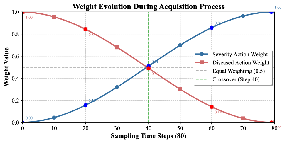
Figure 3: Step-wise weighting evolution for multi-objective diagnosis following lexicographic ordering. The step-wise weight dynamically determines the preference of the reward feedback in disease detection and severity quantification objectives, which ensures a smooth transition.

Table 1: Objectives, Diagnostic Support, and Inference Data of Implemented Methods. The objective of Policy Recon is image reconstruction

	Diagnostic Objectives			Diagnostic Strengths		Data Used for Inference
Method	Disease Detection	Severity Quantification	Overall Diagnosis	Sampling Optimization	Sequential Diagnosis	Undersampled $k$-space	Full $k$-space
Fully Sampled	$\circ$	$\circ$	$\circ$				$\checkmark$
Undersampled	$\circ$	$\circ$				$\checkmark$
Policy Recon [18]	-	-	-	$\checkmark$		$\checkmark$
Policy Classifier [4]	$\circ$	$\circ$		$\checkmark$		$\checkmark$
Simulated Policy			$\circ$	$\checkmark$		$\checkmark$
Varying Parameter Policy	$\bullet$	$\bullet$		$\checkmark$		$\checkmark$
Weighted Policy (Ours)	$\bullet$	$\bullet$	$\bullet$	$\checkmark$	$\checkmark$	$\checkmark$
$\circ$ : Objective optimized independently (one objective per strategy) $\bullet$ : Multiple objectives optimized simultaneously within a single strategy

4 Experimental Setup

4.1 Dataset and Pre-processing

Dataset: Experiments are conducted with the single-coil $k$-space data and slice-level labels from the publicly available fastMRI dataset [34] and fastMRI+ dataset [35]. We use $1,172$ annotated volumes from the fastMRI Knee dataset to validate the performance of our framework in two types of pathology diagnosis and severity quantification: ACL Sprain (High Grade/Low-Moderate Grade) and Cartilage Thickness Loss (Full/Partial). We follow the data split provided by the dataset, resulting in the distribution of Table 2.

Table 2: Train-Val-Test Split for ACL Sprain and Cartilage Thickness Loss datasets

Pathology	ACL Sprain			Cartilage Thickness Loss
Severity Degree	No Finding	Low-Mod Grade	High Grade	No Finding	Partial	Full
Train	$30915$	$617$	$503$	$29768$	$1850$	$417$
Validation	$5180$	$56$	$58$	$4907$	$325$	$62$
Test	$1734$	$42$	$65$	$1732$	$79$	$30$
Total	$37829$	$715$	$626$	$36407$	$2254$	$509$

Data Pre-processing: Since the $k$-space data have varying sizes, we first apply inverse Fourier transform to obtain the fully sampled $k$-space data to get the ground truth image and crop it to size $(320\times 320)$ for computational efficiency. After applying Fourier transform to the ground truth image, we obtain the ground truth $k$-space data. There is a severe class imbalance between the two diagnostic tasks. To address it during training, we use weighted cross-entropy loss based on the label distribution to avoid overfitting to the majority class and poor generalization on the minority class. When training the policy network, we undersample the data for computational savings, as suggested in [18, 4].

4.2 Baselines and Benchmarks

We design benchmark methods and baselines based on different diagnostic strengths, data access, and objectives as shown in Table 1, to fairly evaluate our approach.

4.2.1 Fully Sampled Classifier (Oracle)

This serves as an oracle benchmark for classifier performance with fully sampled $k$-space data as input, and hence no sampling optimization occurs. We trained the disease classifier with the ground truth images which are derived from fully sampled $k$-space data and supervised by the disease level label. The severity classifier is fine-tuned from the well-trained disease classifier with only diseased subjects and their severity label. The sequential diagnosis results are inferred by connecting disease and severity classifiers together. We refer to it as Fully Sampled.

4.2.2 Undersampled Classifier

The classifier serves as a baseline for single binary tasks, such as disease diagnosis and severity quantification, with the inverse Fourier transform applied to the randomly undersampled $k$-space data and no sampling optimization. It adopts the same backbone as the Oracle and is trained with undersampled images with various sample rates ($5\%$ to $30\%$) and center fraction ($0\%$ to $5\%$), supervised as before. We refer to it as Undersampled.

4.2.3 Single-task Oriented Methods

The methods introduced here are designed for single-task evaluation, targeting binary diagnosis of disease detection or severity quantification.

Policy Classifier [4]: This diagnosis-oriented policy benchmark optimizes patient-level sampling in $k$-space for direct inference, setting the upper bound for disease detection and severity quantification. For disease detection, we use a backbone similar to Undersampled as a pre-trained classifier. For severity quantification, the classifier is fine-tuned from the disease detection model. Sampling policy rewards are computed via weighted cross-entropy predictions, with feature maps from the pre-trained classifier as input to the policy network. Training starts with a $5\%$ initial sample rate, progressively sampling $80$ lines to reach a $30\%$ budget.

Policy (via) Reconstruction [18]: This model optimizes patient-level sampling with image reconstruction error as rewards, providing a comparison when reconstruction is involved in diagnosis. We pre-train a U-Net [36] with a $16$-channel first feature map and $4$ pooling cascades, totaling $837\mathrm{K}$ parameters. The model is trained across sampling rates ($5\%$–$30\%$) with a $5\%$ center fraction, supervised using $\ell_{1}$ loss. The active sampler, built on the reconstruction model, uses reconstructed images as input and optimizes sampling with SSIM [37] as the reward. This cascaded design totals $26.7\mathrm{M}$ parameters. Its diagnostic evaluation adopts the Oracle classifiers, which are trained to make predictions from fully sampled images, leading to the Policy-based Reconstruction Network (Policy Recon).

4.2.4 Multi-task oriented Methods for Comprehensive Diagnosis

These diagnosis-oriented methods are designed for multi-task evaluation, aiming to provide a comprehensive diagnosis of the presence and severity of disease. These methods do not consider the order of objectives and enforce sequential steps.

Simulated Policy Classifier: This benchmark evaluates a single-objective reinforcement learning (RL) policy network tailored for comprehensive diagnosis. It adopts a similar architecture to our framework, e.g., extracting the high-level features from the pre-trained disease and severity classifiers, while using a different rewarding mechanism. Instead of relying on step-wise weighting to adjust the diagnostic rewards, this policy is optimized via a reward function that unifies the diagnostic outcomes as the F1-score of a three-class classification task, where the final diagnosis is categorized as: (0) no findings, (1) diseased with low severity, and (2) diseased with high severity. This formulation simulates the situation where the model simultaneously infers both the presence and severity of disease, without enforcing sequential steps. We refer to this approach as Simulated Policy.

Varying Parameter Policy Classifier: To benchmark diagnosis using multi-objective reinforcement learning (MORL) without specifying the optimization order of objectives, we introduce a method based on the varying parameter approach [38]. This method employs two separate policy networks—one for disease detection and another for severity quantification—designing sampling trajectories independently before averaging their outputs to guide $k$-space selection. Each policy is trained with its individual reward, but during joint training, the severity policy considers rewards only from diseased subjects, ignoring others. This approach is termed Varying Parameter Policy.

4.2.5 Weighted Sequential Policy Classifier (Ours)

Our proposed method, introduced in Section 3 is a MORL-based policy network coupled with a step-wise weighting mechanism. The pre-trained disease classifier shares the same backbone as Undersampled and only has access to undersampled $k$-space data. The severity classifier is fine-tuned from the well-trained disease classifier. Both classifiers are utilized to provide step-wise weighting rewards and high-level feature representations to the policy network as illustrated in Figure 2. During joint training, only when the input subject is diseased does the severity reward from the classifier get used. Our method is referred to as Weighted Policy.

4.3 Evaluation Metrics

To assess diagnostic performance, we evaluate our method from three perspectives: disease detection, severity quantification, and overall sequential diagnosis, using Area Under the Receiver Operating Characteristic curve and Balanced Accuracy as primary metrics. For disease detection, we assess the model’s ability to distinguish pathological cases from no findings. Severity quantification focuses on positive cases, evaluating accuracy in classifying disease progression (Low-Moderate vs. High Grade for ACL Sprain; Partial vs. Full for Cartilage Thickness Loss). Sequential diagnosis treats the process as trajectory prediction, requiring correct classification at both stages—detecting disease and assessing severity—for a prediction to be valid, aligning with real-world clinical needs.

4.4 Implementation Details

All classification networks employed share the same ResNet-50 [39] backbone with $25.6\mathrm{M}$ parameters. To avoid overfitting caused by class imbalance, a dropout layer is added at the end, and weighted cross-entropy is used as the supervised learning loss [40]. For methods involving a policy with greedy actions, we use the policy gradient network ($11\mathrm{M}$ parameters) [4, 18] with parallel acquisition $q=8$. For all methods, we employ the Adam optimizer [41] with a learning rate of $10^{-4}$ and a step-based scheduler with a decay gamma of $0.1$ for all model training. All disease classification and reconstruction models are trained for $50$ epochs, and the severity classification model is fine-tuned for $20$ epochs. For the policy model, we train it for $30$ epochs. Our experimental setup uses the PyTorch framework, and all computations are performed on an NVIDIA A100 Tensor Core GPU.

Table 3: Average balanced accuracy (%) and Area Under Curve (%) results and the standard deviations of different diagnostic policies across varying sampling rates for ACL Sprain Diagnosis. Dashes (—) indicate scenarios where the method is not applicable. Bold numbers denote the best performance

Balanced Accuracy $\uparrow$
Diagnosis Task	Disease					Severity Degree					Sequential Diagnosis
Fully Sampled (Oracle)			$\textbf{84.27}_{0.0}$					$\textbf{69.20}_{1.5}$					$\textbf{65.94}_{0.1}$
Sampling Rate	5%	10%	15%	20%	30%	5%	10%	15%	20%	30%	5%	10%	15%	20%	30%
Undersampled	$72.90_{2.9}$	$75.68_{2.5}$	$76.14_{1.9}$	$76.58_{1.8}$	$79.64_{0.8}$	$\textbf{60.62}_{1.7}$	$61.20_{3.0}$	$62.90_{3.1}$	$64.58_{4.0}$	$68.42_{2.5}$	—	—	—	—	—
Policy Classifier [4]	$72.90_{2.9}$	$81.32_{1.7}$	$81.78_{1.4}$	$81.84_{0.7}$	$82.94_{0.8}$	$\textbf{60.62}_{1.7}$	$71.94_{2.7}$	$74.08_{2.3}$	$\textbf{74.64}_{1.9}$	$\textbf{78.58}_{2.6}$	—	—	—	—	—
Policy Recon [18]	$62.54_{0.1}$	$69.60_{0.4}$	$78.60_{0.4}$	$79.14_{0.2}$	$81.92_{0.5}$	$37.70_{0.0}$	$30.32_{1.9}$	$43.08_{2.7}$	$49.14_{0.1}$	$54.64_{2.1}$	$41.90_{0.0}$	$39.68_{0.7}$	$52.44_{1.7}$	$55.22_{0.1}$	$60.40_{1.1}$
Weighted Policy (Ours)	$\textbf{73.26}_{2.8}$	$\textbf{84.20}_{1.3}$	$\textbf{84.76}_{1.0}$	$\textbf{84.34}_{0.7}$	$\textbf{83.54}_{0.4}$	$58.94_{4.1}$	$\textbf{76.86}_{2.8}$	$\textbf{74.10}_{3.1}$	$73.88_{1.9}$	$75.36_{2.8}$	$\textbf{53.58}_{3.1}$	$\textbf{73.42}_{2.0}$	$\textbf{72.36}_{1.9}$	$\textbf{71.72}_{1.7}$	$\textbf{71.68}_{1.6}$
Area Under Curve $\uparrow$
Diagnosis Task	Disease					Severity Degree					Sequential Diagnosis
Fully Sampled (Oracle)			$\textbf{90.23}_{0.0}$					$\textbf{71.03}_{1.2}$					$\textbf{80.76}_{0.1}$
Sampling Rate	5%	10%	15%	20%	30%	5%	10%	15%	20%	30%	5%	10%	15%	20%	30%
Undersampled	$\textbf{84.10}_{1.8}$	$85.58_{1.3}$	$86.50_{1.2}$	$87.28_{1.3}$	$88.40_{0.7}$	$\textbf{69.20}_{4.6}$	$70.34_{5.5}$	$73.38_{4.5}$	$75.36_{4.2}$	$79.70_{4.7}$	—	—	—	—	—
Policy Classifier [4]	$\textbf{84.10}_{1.8}$	$88.72_{0.5}$	$88.64_{0.5}$	$88.54_{0.4}$	$88.98_{0.4}$	$\textbf{69.20}_{4.6}$	$83.78_{1.7}$	$84.80_{1.3}$	$85.10_{1.4}$	$87.16_{1.5}$	—	—	—	—	—
Policy Recon [18]	$78.16_{0.1}$	$84.02_{0.1}$	$87.98_{0.0}$	$88.44_{0.1}$	$89.30_{0.1}$	$35.80_{0.0}$	$25.40_{0.5}$	$42.10_{0.9}$	$46.66_{0.4}$	$57.86_{0.9}$	$56.98_{0.0}$	$54.72_{0.3}$	$65.02_{0.4}$	$67.56_{0.2}$	$73.58_{0.4}$
Weighted Policy (Ours)	$83.24_{1.5}$	$\textbf{89.32}_{0.4}$	$\textbf{89.54}_{0.2}$	$\textbf{89.50}_{0.1}$	$\textbf{89.36}_{\textbf{0.3}}$	$67.22_{5.5}$	$\textbf{88.14}_{1.2}$	$\textbf{86.76}_{1.4}$	$\textbf{86.08}_{1.0}$	$\textbf{87.44}_{1.1}$	$\textbf{75.22}_{3.0}$	$\textbf{88.72}_{0.6}$	$\textbf{88.14}_{0.8}$	$\textbf{87.78}_{0.5}$	$\textbf{88.40}_{0.7}$

Table 4: Same as in Table 3 but for Cartilage Thickness Loss

Balanced Accuracy $\uparrow$
Diagnosis Task	Disease					Severity Degree					Sequential Diagnosis
Fully Sampled (Oracle)			$\textbf{75.05}_{0.1}$					$\textbf{60.90}_{2.7}$					$\textbf{54.84}_{0.0}$
Sampling Rate	5%	10%	15%	20%	30%	5%	10%	15%	20%	30%	5%	10%	15%	20%	30%
Undersampled	$71.12_{3.0}$	$73.22_{1.2}$	$74.32_{0.9}$	$74.62_{1.4}$	$75.22_{1.4}$	$54.90_{2.3}$	$59.42_{3.0}$	$59.02_{3.0}$	$60.32_{3.3}$	$61.38_{2.8}$	—	—	—	—	—
Policy Classifier [4]	$71.12_{3.0}$	$\textbf{73.72}_{2.5}$	$\textbf{75.14}_{1.1}$	$\textbf{75.30}_{1.3}$	$\textbf{75.98}_{1.2}$	$54.90_{2.3}$	$58.58_{4.0}$	$\textbf{60.30}_{1.4}$	$\textbf{63.10}_{3.9}$	$\textbf{63.84}_{5.0}$	—	—	—	—	—
Policy Recon [18]	$64.34_{0.1}$	$65.86_{0.9}$	$72.18_{0.3}$	$71.20_{0.3}$	$75.92_{0.4}$	$56.58_{0.0}$	$56.68_{1.0}$	$54.50_{0.9}$	$55.18_{0.0}$	$56.60_{0.9}$	$45.22_{0.0}$	$44.72_{1.3}$	$50.18_{0.7}$	$50.16_{0.1}$	$54.46_{0.7}$
Weighted Policy (Ours)	$\textbf{72.76}_{1.5}$	$72.96_{1.0}$	$74.02_{0.9}$	$73.86_{1.1}$	$73.84_{1.5}$	$\textbf{58.92}_{5.7}$	$\textbf{60.62}_{3.9}$	$58.98_{2.8}$	$60.88_{2.5}$	$62.32_{3.0}$	$\textbf{54.40}_{2.8}$	$\textbf{54.88}_{2.1}$	$\textbf{53.90}_{2.2}$	$\textbf{54.80}_{0.9}$	$\textbf{55.48}_{0.6}$
Area Under Curve $\uparrow$
Diagnosis Task	Disease					Severity Degree					Sequential Diagnosis
Fully Sampled (Oracle)			$\textbf{88.23}_{0.0}$					$\textbf{73.58}_{4.2}$					$\textbf{80.88}_{0.5}$
Sampling Rate	5%	10%	15%	20%	30%	5%	10%	15%	20%	30%	5%	10%	15%	20%	30%
Undersampled	$84.58_{1.0}$	$86.02_{0.7}$	$87.38_{0.3}$	$87.86_{0.7}$	$88.08_{0.6}$	$61.90_{5.0}$	$66.40_{7.4}$	$68.76_{5.3}$	$71.80_{5.4}$	$76.82_{4.5}$	—	—	—	—	—
Policy Classifier [4]	$84.58_{1.0}$	$86.74_{0.4}$	$87.32_{0.4}$	$87.82_{0.4}$	$87.96_{0.4}$	$61.90_{5.0}$	$\textbf{81.12}_{2.0}$	$\textbf{83.10}_{1.6}$	$83.24_{1.3}$	$85.26_{1.4}$	—	—	—	—	—
Policy Recon [18]	$83.72_{0.0}$	$85.30_{0.1}$	$86.18_{0.1}$	$86.42_{0.0}$	$87.38_{0.1}$	$\textbf{71.44}_{0.1}$	$68.32_{0.9}$	$71.30_{0.6}$	$70.52_{0.6}$	$75.00_{0.9}$	$\textbf{77.58}_{0.0}$	$76.84_{0.4}$	$78.74_{0.3}$	$78.48_{0.3}$	$81.22_{0.4}$
Weighted Policy (Ours)	$\textbf{85.24}_{0.8}$	$\textbf{87.34}_{0.3}$	$\textbf{89.06}_{0.4}$	$\textbf{88.98}_{0.3}$	$\textbf{89.02}_{0.3}$	$65.70_{6.1}$	$75.04_{1.2}$	$80.94_{1.6}$	$\textbf{83.60}_{1.0}$	$\textbf{85.58}_{1.5}$	$75.44_{3.2}$	$\textbf{81.20}_{0.6}$	$\textbf{84.98}_{0.8}$	$\textbf{86.28}_{0.6}$	$\textbf{87.26}_{0.8}$

5 Experimental Results and Analysis

We divide this section into several parts, each addressing key questions/hypotheses. First, we aim to show that our approach maintains diagnostic performance when compared to other non-sequential and single objective policies. We then proceed to address our main hypothesis that adopting sequential decisions leads to $k$-space savings. Finally, we show that the natural ordering of the objectives results in even more savings.

5.1 Comparison to Non-sequential and Single Objective Policies

In this section, we first answer a critical question: Will our method compromise performance when enforcing multiple objectives in a single scan? We compare the diagnostic accuracy of our sequential diagnosis method with baselines and benchmarks designed for a single binary diagnosis task, namely the Undersampled, Policy Recon, and Policy Classifier, at various sample rates for inferring the conditions of ACL Sprain and Cartilage Thickness Loss. Undersampled randomly samples $k$-space lines progressively. Policy Recon, Policy Classifier, and Weighted Policy start with a randomly initialized mask at a sample rate of $5\%$ and perform sampling decision-making respectively using their policies (see Section 4.2). We also include Fully sampled as a diagnostic oracle, which does not have a sampling budget. The results are shown in Table 3 and Table 4.

Our Weighted Policy, consistently demonstrates strong performance in all metrics across different sampling rates and both tasks (ACL Sprain and Thickness Loss). Focusing first on Table 3, we observe that: (i) Weighted Policy matches the performance of Fully Sampled, showing that careful selection of $k$-space lines avoids taking redundant and irrelevant information. (ii) The advantage of policy-based optimization in our method is clearly demonstrated as we can match the performance of Fully Sampled with roughly $10\%$ $k$-space data across all subtasks. (iii) As expected, Policy Recon, which optimizes reconstruction performance, underperforms our approach which optimizes for each task at hand. (iv) More importantly, our Weighted Policy, which jointly optimizes disease detection and severity quantification, outperforms the Policy Classifier in most cases even when used for a single subtask with fewer samples. In fact, with $10\%$ sampling in disease detection ($84.20\%$ vs. $81.32\%$) and $20\%$ $k$-space sampling for severity quantification ($74.10\%$ vs. $74.08\%$), this finding is extremely important, as it answers the initially posed question. It demonstrates that a policy optimized for multiple objectives does not compromise diagnostic performance compared to policies optimized for a single objective.

Similar observations hold for Cartilage Thickness Loss in Table 4, evidently illustrating the applicability of our methods in two settings and hence the strength of our findings.

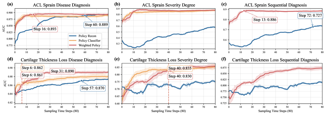
Figure 4: Performance comparison of our proposed Weighted Policy and two single-task oriented policies. The horizontal axis indicates the cumulative lines acquired when sampling. The $80$-step active sampling procedure starts from $16$ randomly sampled $k$-space lines.

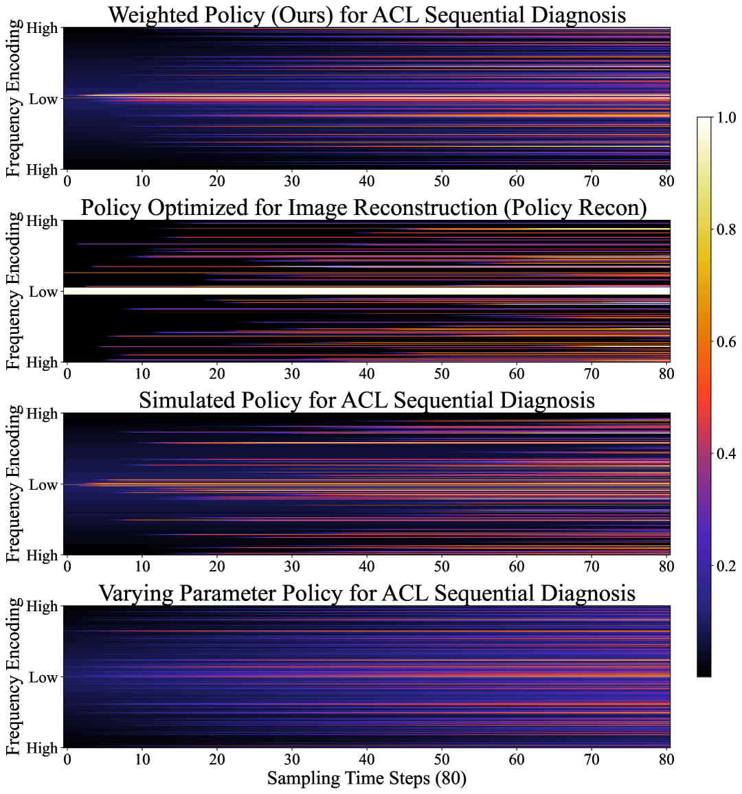
Figure 5: Average $k$-space sampling behaviors across all subjects of our proposed Weighted Policy and benchmarks. A High value in the plot represents a high probability to be sampled. The horizontal axis indicates the cumulative lines acquired when sampling.

5.2 k-space Savings

We now proceed to answer our main hypothesis: Joint optimization of a policy for two objectives ultimately leads to sampling efficiency and savings.

In Figure 4, we illustrate the diagnostic performance of policies that progressively make decisions on which line to acquire, line-by-line, and visualize their sampling trajectories. We present the performance of our method and compare with Policy Recon and Policy Classifier to showcase the difference between sampling patterns of single-task methods versus ours.

We find that the performance curve plateaus during the sampling process, indicating that the policies might have collected the majority of diagnostically significant $k$-space lines that contribute to diagnostic performance enhancement.

For disease detection, as shown in Figure 4 (a) and (d), compared to Policy Recon which optimizes sampling trajectories for reconstruction, our method plateaus earlier at step $16$ for ACL Sprain, whereas Policy Recon plateaus much later (at step $60$ for ACL Sprain leading to considerate $k$-space savings. The advantage of a diagnosis-oriented policy is further highlighted in severity quantification (Figure 4 (b)), where our method successfully identifies $k$-space lines that can significantly improve inference. In contrast, although it can achieve continuous improvements in reconstruction performance, Policy Recon struggles to effectively locate diagnostically relevant $k$-space lines and produce comparable outcomes in both severity and sequential diagnosis classification. Consequently, when evaluating sequential diagnosis in ACL Sprain (Figure 4 (c)), our method reaches a plateau at step $13$ with a high balanced accuracy of $0.886$, while Policy Recon arrives at step $72$ with a balanced accuracy of $0.727$. Similar observations hold for Cartilage Thickness Loss (Figure 4 (d) to (f)).

In Figure 4, compared to the policies of Policy Classifier that optimize sampling trajectories independently for separate tasks (disease detection or severity quantification), our method provides competitive results and achieves considerate acquisition savings. For ACL Sprain, our policy quickly matches the performance of Policy Classifiers, and exceeds them afterward. Similarly, as shown in plots (d) and (e), Weighted Policy samples $6$ lines in disease detection and $40$ lines in severity quantification for Cartilage Thickness Loss to achieve the performance of the corresponding Policy Classifier. Notably, our policy achieves this sequentially whereas the other policies require different sessions for two tasks. Hence, our method can significantly reduce the quantity of necessary $k$-space lines and thereby shorten the acquisition time.

Next, we want to compare the sampling behaviors of different policies averaged across the subject population. As shown in Figure 5, referring to the top two plots, there are evident differences between the trajectories of Policy Recon and Weighted Policy. Policy Recon tends to consistently sample low-frequency central $k$-space lines, whereas our method shows a broader diversity (across the frequency spectrum), illustrating its adaptation at the patient level.

5.3 Sequential Diagnosis in One Scanning Session

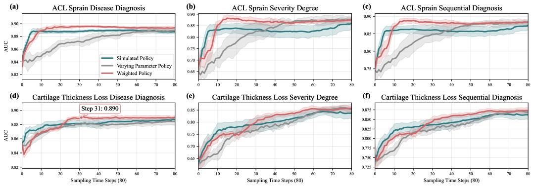
Figure 6: Performance comparison of our proposed Weighted Policy and two multi-task oriented policies. The horizontal axis indicates the cumulative lines acquired when sampling. The $80$-step active sampling procedure starts from $16$ randomly sampled $k$-space lines.

We base our work on a key question: Is it necessary to adopt a sequential process, detecting disease first and then assessing severity? This question is crucial because our proposed sequential diagnosis workflow employs the lexicographic ordering in step-wise weighting module, attempting to mirror the clinical workflow of radiologists. To address this key question, we train two policies with different ways to optimize for multiple objectives in parallel and independently. The first, termed Simulated Policy, uses the same architecture as ours but employs a single-objective RL algorithm rewarded by the performance of a three-way diagnosis (no finding, low, or high severity) without specifying the lexicographic ordering among diagnostic objectives. The second, the Varying Parameter Policy, is instead a MORL-based method, which uses separate policy networks to optimize detection and quantification in parallel as independent objectives, and the final sampling policy is the average of the result of the two policy networks.

Referring to Figure 6 and first focusing on comparisons with the Simulated Policy, we see that the Simulated Policy plateaus earlier at a lower performance compared to our method. This is because the Simulated Policy is rewarded based on overall sequential diagnosis improvements, forcing the policy to find $k$-space lines that contribute to a three-way objective, therefore lacking reward information for each independent objective. Our method explicitly calculates the separate rewards of the two objectives, which simplifies the sequential diagnosis task and reduces the complexity of the sampling strategy optimization.

We compare with Varying Parameter Policy, a MORL-based trained policy, whose key differences are: (i) it employs individual policies to process rewards from the independent objectives in parallel; and most importantly, (ii) it does not utilize the lexicographic ordering between objectives. Thus, we expect to observe worse performance for this ‘simpler’ policy. Looking again at Figure 6, and now comparing the ‘grey’ (Varying Parameter Policy) and ‘red’ (Weighted Policy) lines, our method outperforms the other policy and plateaus earlier at a higher accuracy level, particularly in the overall sequential diagnosis (Figure 6 (c) and (f)), hence achieving $k$-space sampling savings and in turn less scanning time. This highlights the benefits of lexicographic ordering in multi-objective optimization and step-wise weighting. Our policy thus learns the inherent shared diagnostic features between disease detection and severity quantification, and is encouraged to seek mutually beneficial lines during sampling. Consequently, in Figure 6 Cartilage Thickness Loss, after sampling what is needed to decide in the presence of disease (shown as plateauing at step $31$ subplot (d), the optimization prioritizes sampling of k-space lines that contribute to severity as observed by an increase in performance in the subplot (e) without compromising disease diagnosis performance (the plateau).

We can observe such transitions also at the level of sampling trajectories in Figure 5 as well. Looking at the bottom two plots and comparing them with the topmost, until sampling step $16$, our proposed policy samples more low-frequency lines (containing structural information) that can contribute to both objectives and patient-level disease-related information (shown as purple in the plot). Then, the policy smoothly shifts to sampling diagnostic features located in high-frequency zone, which may contribute to severity quantification for ACL Sprain. While Varying Parameter Policy tends to find patient-level features from the start, it can miss the mutual diagnostically significant lines between disease detection and severity quantification. The probability trajectories of the Simulated Policy show several frequency locations with high sampling probability, illustrating a tendency to generate similar sampling trajectories for all subjects, thereby lacking exploration of patient-level diagnostic information.

6 Discussions and Conclusion

6.1 Clinical Relevance

Our framework enables the efficient acquisition of diagnostically relevant $k$-space data while sequentially performing disease detection and severity quantification in a single scanning session. This approach enables comprehensive assessment during the scanning process, potentially eliminating the need for follow-up examinations. The sequential diagnosis paradigm completes multi-objective diagnostic tasks within a single scanning session without requiring full $k$-space acquisition, thereby significantly reducing MRI acquisition time.

The acquisition acceleration of the proposed pipeline via patient-level active sampling could substantially enhance the clinical utility of low-field MRI, making them more viable for PoC applications [1]. We envision practical implementations in preliminary screening scenarios where rapid assessments are crucial to guide resource allocation decisions [42], which is particularly valuable in settings with limited healthcare infrastructure or in emergency medicine contexts [43] where time-critical diagnostic information is essential.

6.2 Limitations

Our method has been implemented as a proof-of-concept on the fastMRI knee dataset, focusing on specific pathologies where data are publicly available. Future work could explore other applications such as stroke [44] or acute brain trauma diagnosis [43], where rapid assessment from limited data is crucial. Although such datasets are not publicly available, we hope our open-source code will encourage researchers with access to evaluate our method in these critical settings.

Our current implementation relies on pre-trained classifiers, which may propagate inherent biases and exhibit vulnerability to domain shifts when applied to new data distributions [45]. An important direction for future research is to explore end-to-end joint optimization of classification and policy networks, potentially through meta-learning approaches that could adapt to new diagnostic tasks with minimal fine-tuning.

6.3 Conclusion

We propose a novel MORL framework for sequential diagnostic assessment directly from undersampled $k$-space data. By structuring clinical diagnosis as a sequential decision process with lexicographic ordering, our method achieves diagnostic performance on par with fully sampled references while significantly reducing acquisition time. Empirical results on two datasets show that our diagnosis-oriented sampling strategy surpasses reconstruction-based methods in both diagnostic accuracy and efficiency. Compared to single-objective diagnostic samplers, our approach achieves substantial $k$-space savings within a single scan without compromising performance. Our step-wise weighting mechanism effectively prioritizes disease detection early in the acquisition before transitioning to severity assessment, thereby aligning with clinical workflows. Furthermore, the convergence of sampling trajectories across tasks supports the existence of shared informative $k$-space regions, enabling efficient, comprehensive assessment in a single session. This work advances direct $k$-space inference, paving the way for clinically viable, PoC MRI diagnostics with reduced acquisition demands.

References

- [1] S. Geethanath and J. T. Vaughan Jr, “Accessible magnetic resonance imaging: a review,” Journal of Magnetic Resonance Imaging, vol. 49, no. 7, pp. e65–e77, 2019.
- [2] Y. Anzai and L. Moy, “Point-of-care low-field-strength mri is moving beyond the hype,” pp. 672–673, 2022.
- [3] M. Hori, A. Hagiwara, M. Goto, A. Wada, and S. Aoki, “Low-field magnetic resonance imaging: its history and renaissance,” Investigative radiology, vol. 56, no. 11, pp. 669–679, 2021.
- [4] Y. Du, R. Dharmakumar, and S. A. Tsaftaris, “The MRI scanner as a diagnostic: image-less active sampling,” in International Conference on Medical Image Computing and Computer-Assisted Intervention. Springer, 2024, pp. 467–476.
- [5] D. J. Lin, P. M. Johnson, F. Knoll, and Y. W. Lui, “Artificial intelligence for mr image reconstruction: an overview for clinicians,” Journal of Magnetic Resonance Imaging, vol. 53, no. 4, pp. 1015–1028, 2021.
- [6] C. D. Bahadir, A. Q. Wang, A. V. Dalca, and M. R. Sabuncu, “Deep-learning-based optimization of the under-sampling pattern in mri,” IEEE Transactions on Computational Imaging, vol. 6, pp. 1139–1152, 2020.
- [7] Z. Zhang, A. Romero, M. J. Muckley, P. Vincent, L. Yang, and M. Drozdzal, “Reducing uncertainty in undersampled mri reconstruction with active acquisition,” in Proceedings of the IEEE/CVF conference on computer vision and pattern recognition, 2019, pp. 2049–2058.
- [8] R. Singhal, M. Sudarshan, A. Mahishi, S. Kaushik, L. Ginocchio, A. Tong, H. Chandarana, D. K. Sodickson, R. Ranganath, and S. Chopra, “On the feasibility of machine learning augmented magnetic resonance for point-of-care identification of disease,” arXiv preprint arXiv:2301.11962, 2023.
- [9] C.-Y. Yen, R. Singhal, U. Sharma, R. Ranganath, S. Chopra, and L. Pinto, “Adaptive sampling of k-space in magnetic resonance for rapid pathology prediction,” arXiv preprint arXiv:2406.04318, 2024.
- [10] G. Zeng, Y. Guo, J. Zhan, Z. Wang, Z. Lai, X. Du, X. Qu, and D. Guo, “A review on deep learning mri reconstruction without fully sampled k-space,” BMC Medical Imaging, vol. 21, no. 1, p. 195, 2021.
- [11] G. Yiasemis, C. I. Sánchez, J.-J. Sonke, and J. Teuwen, “On retrospective k-space subsampling schemes for deep mri reconstruction,” Magnetic Resonance Imaging, vol. 107, pp. 33–46, 2024.
- [12] J. Wang, Q. Yang, Q. Yang, L. Xu, C. Cai, and S. Cai, “Joint optimization of cartesian sampling patterns and reconstruction for single-contrast and multi-contrast fast magnetic resonance imaging,” Computer Methods and Programs in Biomedicine, vol. 226, p. 107150, 2022.
- [13] J. Zhang, H. Zhang, A. Wang, Q. Zhang, M. Sabuncu, P. Spincemaille, T. D. Nguyen, and Y. Wang, “Extending loupe for k-space under-sampling pattern optimization in multi-coil mri,” in Machine Learning for Medical Image Reconstruction: Third International Workshop, MLMIR 2020, Held in Conjunction with MICCAI 2020, Lima, Peru, October 8, 2020, Proceedings 3. Springer, 2020, pp. 91–101.
- [14] G. Wang, T. Luo, J.-F. Nielsen, D. C. Noll, and J. A. Fessler, “B-spline parameterized joint optimization of reconstruction and k-space trajectories (bjork) for accelerated 2d mri,” IEEE Transactions on Medical Imaging, vol. 41, no. 9, pp. 2318–2330, 2022.
- [15] G. Wang and J. A. Fessler, “Efficient approximation of jacobian matrices involving a non-uniform fast fourier transform (nufft),” IEEE transactions on computational imaging, vol. 9, pp. 43–54, 2023.
- [16] S. Ravula, B. Levac, A. Jalal, J. I. Tamir, and A. G. Dimakis, “Optimizing sampling patterns for compressed sensing mri with diffusion generative models,” arXiv preprint arXiv:2306.03284, 2023.
- [17] K. Xuan, S. Sun, Z. Xue, Q. Wang, and S. Liao, “Learning mri k-space subsampling pattern using progressive weight pruning,” in Medical Image Computing and Computer Assisted Intervention–MICCAI 2020: 23rd International Conference, Lima, Peru, October 4–8, 2020, Proceedings, Part II 23. Springer, 2020, pp. 178–187.
- [18] T. Bakker, H. van Hoof, and M. Welling, “Experimental design for MRI by greedy policy search,” Advances in Neural Information Processing Systems, vol. 33, pp. 18 954–18 966, 2020.
- [19] L. Pineda, S. Basu, A. Romero, R. Calandra, and M. Drozdzal, “Active mr k-space sampling with reinforcement learning,” in International Conference on Medical Image Computing and Computer-Assisted Intervention. Springer, 2020, pp. 23–33.
- [20] J. Schlemper, O. Oktay, W. Bai, D. C. Castro, J. Duan, C. Qin, J. V. Hajnal, and D. Rueckert, “Cardiac mr segmentation from undersampled k-space using deep latent representation learning,” in Medical Image Computing and Computer Assisted Intervention–MICCAI 2018: 21st International Conference, Granada, Spain, September 16-20, 2018, Proceedings, Part I. Springer, 2018, pp. 259–267.
- [21] Y. Zhao, X. Wang, T. Che, G. Bao, and S. Li, “Multi-task deep learning for medical image computing and analysis: A review,” Computers in Biology and Medicine, vol. 153, p. 106496, 2023.
- [22] H. Huang, G. Yang, W. Zhang, X. Xu, W. Yang, W. Jiang, and X. Lai, “A deep multi-task learning framework for brain tumor segmentation,” Frontiers in oncology, vol. 11, p. 690244, 2021.
- [23] C. Yu, J. Liu, S. Nemati, and G. Yin, “Reinforcement learning in healthcare: A survey,” ACM Computing Surveys (CSUR), vol. 55, no. 1, pp. 1–36, 2021.
- [24] W. Han, C. Kim, D. Ju, Y. Shim, and S. J. Hwang, “Advancing text-driven chest x-ray generation with policy-based reinforcement learning,” in International Conference on Medical Image Computing and Computer-Assisted Intervention. Springer, 2024, pp. 56–66.
- [25] A. Vlontzos, A. Alansary, K. Kamnitsas, D. Rueckert, and B. Kainz, “Multiple landmark detection using multi-agent reinforcement learning,” in Medical Image Computing and Computer Assisted Intervention–MICCAI 2019: 22nd International Conference, Shenzhen, China, October 13–17, 2019, Proceedings, Part IV 22. Springer, 2019, pp. 262–270.
- [26] D. Zhang, B. Chen, and S. Li, “Sequential conditional reinforcement learning for simultaneous vertebral body detection and segmentation with modeling the spine anatomy,” Medical image analysis, vol. 67, p. 101861, 2021.
- [27] S. N. Khatami and C. Gopalappa, “A reinforcement learning model to inform optimal decision paths for hiv elimination,” Mathematical biosciences and engineering: MBE, vol. 18, no. 6, p. 7666, 2021.
- [28] X. Liao, W. Li, Q. Xu, X. Wang, B. Jin, X. Zhang, Y. Wang, and Y. Zhang, “Iteratively-refined interactive 3d medical image segmentation with multi-agent reinforcement learning,” in Proceedings of the IEEE/CVF conference on computer vision and pattern recognition, 2020, pp. 9394–9402.
- [29] E. J. Sondik, The optimal control of partially observable Markov processes. Stanford University, 1971.
- [30] W. Kool, H. van Hoof, and M. Welling, “Buy 4 REINFORCE samples, get a baseline for free!” 2019. [Online]. Available: https://openreview.net/forum?id=r1lgTGL5DE
- [31] R. C. of Radiologists, “Standards for interpretation and reporting of imaging investigations,” 2018.
- [32] J. Skalse, L. Hammond, C. Griffin, and A. Abate, “Lexicographic multi-objective reinforcement learning,” arXiv preprint arXiv:2212.13769, 2022.
- [33] E. Maeland, “On the comparison of interpolation methods,” IEEE Transactions on Medical Imaging, vol. 7, no. 3, pp. 213–217, 1988.
- [34] J. Zbontar, F. Knoll, A. Sriram, T. Murrell, Z. Huang, M. J. Muckley, A. Defazio, R. Stern, P. Johnson, M. Bruno et al., “fastmri: An open dataset and benchmarks for accelerated mri,” arXiv preprint arXiv:1811.08839, 2018.
- [35] R. Zhao, B. Yaman, Y. Zhang, R. Stewart, A. Dixon, F. Knoll, Z. Huang, Y. W. Lui, M. S. Hansen, and M. P. Lungren, “fastmri+, clinical pathology annotations for knee and brain fully sampled magnetic resonance imaging data,” Scientific Data, vol. 9, no. 1, p. 152, 2022.
- [36] O. Ronneberger, P. Fischer, and T. Brox, “U-net: Convolutional networks for biomedical image segmentation,” in Medical image computing and computer-assisted intervention–MICCAI 2015: 18th international conference, Munich, Germany, October 5-9, 2015, proceedings, part III 18. Springer, 2015, pp. 234–241.
- [37] Z. Wang, A. C. Bovik, H. R. Sheikh, and E. P. Simoncelli, “Image quality assessment: from error visibility to structural similarity,” IEEE transactions on image processing, vol. 13, no. 4, pp. 600–612, 2004.
- [38] C. Liu, X. Xu, and D. Hu, “Multiobjective reinforcement learning: A comprehensive overview,” IEEE Transactions on Systems, Man, and Cybernetics: Systems, vol. 45, no. 3, pp. 385–398, 2014.
- [39] K. He, X. Zhang, S. Ren, and J. Sun, “Deep residual learning for image recognition,” in Proceedings of the IEEE conference on computer vision and pattern recognition, 2016, pp. 770–778.
- [40] A. Mao, M. Mohri, and Y. Zhong, “Cross-entropy loss functions: Theoretical analysis and applications,” in Proceedings of the 40th International Conference on Machine Learning, ser. Proceedings of Machine Learning Research, vol. 202. PMLR, 2023, pp. 23 803–23 828.
- [41] D. P. Kingma and J. Ba, “Adam: A method for stochastic optimization,” arXiv preprint arXiv:1412.6980, 2014.
- [42] A. P. Brady, J. A. Bello, L. E. Derchi, M. Fuchsjäger, S. Goergen, G. P. Krestin, E. J. Lee, D. C. Levin, J. Pressacco, V. M. Rao et al., “Radiology in the era of value-based healthcare: a multi-society expert statement from the acr, car, esr, is3r, ranzcr, and rsna,” Canadian Association of Radiologists Journal, vol. 72, no. 2, pp. 208–214, 2021.
- [43] M. H. Mazurek, B. A. Cahn, M. M. Yuen, A. M. Prabhat, I. R. Chavva, J. T. Shah, A. L. Crawford, E. B. Welch, J. Rothberg, L. Sacolick et al., “Portable, bedside, low-field magnetic resonance imaging for evaluation of intracerebral hemorrhage,” Nature communications, vol. 12, no. 1, p. 5119, 2021.
- [44] K. C. Ho, F. Scalzo, K. V. Sarma, W. Speier, S. El-Saden, and C. Arnold, “Predicting ischemic stroke tissue fate using a deep convolutional neural network on source magnetic resonance perfusion images,” Journal of Medical Imaging, vol. 6, no. 2, pp. 026 001–026 001, 2019.
- [45] C. Wachinger, A. Rieckmann, S. Pölsterl, A. D. N. Initiative et al., “Detect and correct bias in multi-site neuroimaging datasets,” Medical Image Analysis, vol. 67, p. 101879, 2021.