Decentralized Nonconvex Optimization under Heavy-Tailed Noise: Normalization and Optimal Convergence

Abstract

Heavy-tailed noise in nonconvex stochastic optimization has garnered increasing research interest, as empirical studies, including those on training attention models, suggest it is a more realistic gradient noise condition. This paper studies first-order nonconvex stochastic optimization under heavy-tailed gradient noise in a decentralized setup, where each node can only communicate with its direct neighbors in a predefined graph. Specifically, we consider a class of heavy-tailed gradient noise that is zero-mean and has only $p$-th moment for $p\in(1,2]$. We propose GT-NSGDm, Gradient Tracking based Normalized Stochastic Gradient Descent with momentum, that utilizes normalization, in conjunction with gradient tracking and momentum, to cope with heavy-tailed noise on distributed nodes. We show that, when the communication graph admits primitive and doubly stochastic weights, GT-NSGDm guarantees, for the first time in the literature, that the expected gradient norm converges at an optimal non-asymptotic rate $O\big{(}1/T^{(p-1)/(3p-2)}\big{)}$, which matches the lower bound in the centralized setup. When tail index $p$ is unknown, GT-NSGDm attains a non-asymptotic rate $O\big{(}1/T^{(p-1)/(2p)}\big{)}$ that is, for $p<2$, topology independent and has a speedup factor $n^{1-1/p}$ in terms of the number of nodes $n$. Finally, experiments on nonconvex linear regression with tokenized synthetic data and decentralized training of language models on a real-world corpus demonstrate that GT-NSGDm is more robust and efficient than baselines.

1 Introduction

In this paper, we address the problem of nonconvex stochastic optimization under heavy-tailed gradient noise in the decentralized setup. Consider a graph with $n$ nodes connected by a predefined topology $\mathcal{G}:=(\mathcal{V},\mathcal{E})$, where $\mathcal{V}:=\{1,\ldots,n\}$ is the set of node indices, and $\mathcal{E}$ is the collection of directed pairs $(i,r)$, $i,r\in\mathcal{V}$ such that node $i$ can send information to the neighboring node $r$. Each node $i\in\mathcal{V}$ holds a local nonconvex differentiable cost function $f_{i}:\mathbb{R}^{d}\rightarrow\mathbb{R}$, and can access its stochastic gradient, subject to zero mean noise with a bounded $p$-th moment for some $p\in(1,2]$. Cooperatively, these nodes aim to solve $\min_{\bm{x}\in\mathbb{R}^{d}}f(\bm{x}):=(1/n)\sum_{i=1}^{n}f_{i}(\bm{x})$, through local computation and peer-to-peer communication only with their immediate neighbors,

Decentralized optimization in the above formulation has been studied for decades [1], and has recently attracted growing research interest due to its advantages in scalability and privacy preservation across a wide range of distributed machine learning, signal processing, and control tasks over networks [2, 3, 4]. For instance, in privacy-sensitive applications such as those in the medical domain [5], training data are often distributed across $n$ nodes due to privacy constraints. In such cases, each $f_{i}$ represents an empirical risk function, e.g., a neural network, defined over the local dataset on node $i$, and all nodes collaboratively train a global predictive model via peer-to-peer communication without sharing raw data. Moreover, decentralized optimization is also employed in data centers to reduce communication bottlenecks associated with the central node in traditional centralized training paradigms [6].

In decentralized optimization, first-order methods are widely favored for their simplicity and scalability[7]. However, computing the exact gradient of each local objective function $f_{i}$ at every iteration can be computationally expensive, particularly in large-scale settings where each node holds a substantial volume of local data. To alleviate this computational burden, decentralized stochastic gradient methods, which approximate exact gradients, have been extensively studied. Most existing approaches, including decentralized stochastic (sub)gradient descent [8, 9, 10], variance reduction techniques [11], and gradient tracking-based schemes [12, 13], typically assume that stochastic gradient noise has a finite variance. Nevertheless, recent empirical and theoretical evidence indicates that, when optimizing certain neural network architectures, especially attention-based models such as Transformers [14], the gradient noise often follows a heavy-tailed distribution with significantly large or even infinite variance [16, 17, 18, 19, 20, 21]. The presence of heavy-tailed gradient noise poses substantial challenges for existing methods. Empirically, some stochastic gradient descent (SGD) based methods can suffer from instability and even dramatic drop of training accuracies [17, 22, 23], particularly in distributed large-cohort training. Theoretically, unbounded variance renders many established analyses invalid, and in centralized settings it necessitates the use of nonlinear adaptive techniques such as clipping, sign, and normalization [17, 24, 25, 26, 27, 28] to combat the strong noise. However, incorporating such adaptive strategies in decentralized algorithms introduces inherent nonlinearity into the algorithmic dynamics associated with the average-sum structured function $f$, making the design and analysis of decentralized algorithms under heavy-tailed noise significantly more challenging.

Decentralized optimization under heavy-tailed gradient noise remains underexplored. To the best of our knowledge, only recent studies [29, 30] have attempted to address this problem under restrictive assumptions. Specifically, [29] considers zero-mean gradient noise with bounded $p$-th central moment ($p\in(1,2]$) similar to our setting but assumes a compact domain, effectively implying bounded gradients. Their proposed decentralized gradient descent method with $\ell_{2}$ gradient clipping achieves almost sure convergence for strongly convex local functions. However, the restrictive compact domain assumption in [29] limits its practical applicability, and the convergence rate is not explicitly provided. Another work, [30], also assumes strongly convex local objectives and develops a decentralized gradient method with smoothed clipping and error feedback under gradient noise that is zero-mean, symmetric, and has bounded first absolute moment, showing an in-expectation convergence rate of $1/t^{\delta}$ for some $\delta\in(0,2/5)$. Although the noise assumption in [30] is weaker than ours (as it requires only a first-moment bound), the additional assumptions of noise symmetry and the dependence of the rate exponent $\delta$ on both the problem dimension and condition number restrict its general applicability. Moreover, both works [29, 30] assume strong convexity, whereas many practical optimization problems involving heavy-tailed noise, particularly in modern machine learning, are inherently nonconvex. Further, the convergence rates in [29, 30] are either unclear or sub-optimal, even compared to the optimal iteration complexity bound $O\big{(}1/T^{(p-1)/(3p-2)}\big{)}$ for general nonconvex functions. In this work, we relax these restrictive assumptions and address the following question:

Can we design a decentralized algorithm for nonconvex optimization under general zero-mean gradient noise with only a finite $p$-th moment for $p\in(1,2]$ with optimal iteration complexity?

1.1 Contributions

We provide a positive answer to the above question through the following key contributions.

• We develop a decentralized method, called GT-NSGDm, using normalization, coupled with momentum variance reduction, to combat heavy-tailed noise, and using gradient tracking to handle cross-node heterogeneity. To further shed light on the design of GT-NSGDm, we provide a negative result for a vanilla variant of normalized decentralized SGD that employs no gradient tracking nor momentum.

• For general nonconvex and smooth local functions $f_{i}$’s that are bounded from below, we show that GT-NSGDm converges in expectation at a rate $O\big{(}1/T^{(p-1)/(3p-2)}\big{)}$, which matches the lower bound in centralized setting and is order-optimal. Our convergence rate significantly improves upon related works [29, 30], which assume strong convexity and either do not provide a convergence rate or lack an explicit rate exponent.

• When the tail index $p$ is unknown, GT-NSGDm achieves a rate of $O(1/T^{(p-1)/(2p)})$, matching the best-known rate in the centralized setting without requiring knowledge of $p$. Notably, for $p\in(1,2)$ and sufficiently large $T$, this rate is independent of the network topology and exhibits a speedup in the number of nodes, with a factor of $n^{1-1/p}$.

• We test our theoretical findings in nonconvex linear regression models on a synthetic dataset that is built to simulate language tokens under controlled heavy-tailed noise injections. We also test GT-NSGDm on distributed training of decoder-only Transformer models on Multi30k datasets [31]. Experiments on multiple variants of network topologies show that GT-NSGDm is more robust to injected and empirical heavy-tailed noise and converges faster.

1.2 Related Work

Heavy-tailed gradient noise. Recent empirical studies suggest that the distribution of gradient noise in training various deep learning models resembles heavy-tailed distributions, such as Lévy’s $\alpha$-stable distribution [16, 17, 32, 33]. For instance, the work [17] demonstrates that the empirical distribution of gradient norm samples during BERT pre-training closely aligns with an $\alpha$-stable distribution, rather than a Gaussian one (see their Figure 1). The presence of heavy-tailed gradient noise is also supported by theoretical insights [16, 34, 19, 32]. In particular, [16] leverages generalized central limit theorems to show that the gradient noise in SGD can converge to an $\alpha$-stable random variable.

Adaptive methods. Under heavy-tailed noise, vanilla SGD based methods are shown to suffer from slower convergence or even model collapses in centralized settings [17] as well as distributed settings with a central server [23, 35], and adaptive methods such as clipping and normalization are introduced to stabilize training dynamics. In centralized settings, the work [17] provides lower bounds for both nonconvex and strongly convex smooth functions, showing that SGD with gradient clipping achieves in-expectation upper bounds matching lower bounds. In [24, 36, 37, 38], the authors show that when equipped with gradient clipping, SGD, accelerated methods, AdaGrad [39], and Adam [40] can achieve (near-)optimal high-probability convergence under various function assumptions. Besides, the work [25] shows that signSGD is also robust to heavy-tailed noise through the lens of stochastic differential equations. Further, SGD with gradient normalization, which advantageously requires less hyper-parameter tuning than clipping, is shown to achieve optimal in-expectation convergence [26, 27, 41]. Our method incorporates the same normalization and variance reduction approach as [27]. Notably, in another line of works [42, 28, 43], the authors conduct a unified convergence analyses for generic nonlinear methods including clipping, sign, and normalization under symmetric noise with positive probability mass around zero without assuming any noise moment bound or only assuming first absolute noise moment bound. In distributed settings with a server, the work [44] proposes an algorithm that incorporates an error feedback mechanism, wherein clipping is applied to the discrepancy between a local gradient estimator and a stochastic gradient, and establishes optimal high-probability bounds. Moreover, the work [45] shows that distributed signSGD converges to an asymptotic neighborhood depending on the ‘fatness’ of noise tail. When multiple local updates are permitted between communication rounds, the authors of [23] show that clipping per local step achieves order-optimal in-expectation convergence, albeit under a restrictive bounded gradient assumption. More recently, the work [35] introduces the TailOPT framework, which adaptively leverages gradient geometry by applying clipping operators during local updates on distributed nodes and utilizing adaptive optimizers for global updates at the server, achieving in-expectation sublinear convergence rates that are independent of the moment parameter $p$.

Nonlinearities in decentralized optimization. Extending existing methods that are robust to heavy-tailed noise, whether developed for centralized settings or distributed settings with a server, to decentralized environments is highly nontrivial, primarily due to the nonlinearities introduced to peer-to-peer communication. This difficulty is reflected in that existing decentralized methods incorporating nonlinear adaptive techniques for other purposes often impose restrictive conditions [46, 47]. For example, to achieve differential privacy through gradient clipping, the work [47] establishes convergence in decentralized setups under the assumption of either bounded gradient or a stringent similarity condition, namely $\|\nabla f_{i}(\bm{x})-\nabla f(\bm{x})\|\leq(1/12)\|\nabla f(\bm{x})\|$ for all $i\in[n]$ and all $\bm{x}$. Similarly, to attain adversarial robustness against gradient attacks, the authors of [46] employ gradient clipping with momentum, assuming that all local functions are convex, share a common minimizer, and that $\sum_{i=1}^{n}f_{i}$ is strongly convex. In this work, we significantly relax these conditions and demonstrate the effective use of nonlinearity (specifically, normalization) in decentralized optimization, thereby motivating broader applications of nonlinear techniques in this setting.

1.3 Paper Outline and Notation

We introduce the problem setup and develop our proposed algorithm GT-NSGDm in Sections 2 and 3, respectively. Then, we present our convergence results in Section 4 and discuss their implications. Section 5 presents our numerical studies, while Section 6 concludes the paper.

We denote by $\mathbb{N}_{+}$, $\mathbb{R}$, $\mathbb{R}_{+}$ and $\mathbb{R}^{d}$, respectively, the set of positive natural numbers, real numbers, nonegative real numbers, and the $d$-dimensional Euclidean space. We use lowercase normal letters for scalars, lowercase boldface letters for vectors, and uppercase boldface letters for matrices. Further, we denote by $\mathbf{1}_{k}$ and $\mathbf{0}_{k}$ the all-ones and all-zeros vectors of size $k$, respectively, and by $\bm{I}_{k}$ the $k\times k$ identity matrix. We let $\|\bm{x}\|$ denote the $\ell_{2}$ norm of $\bm{x}$, and $\|\bm{A}\|_{2}$ denote the operator norm of $\bm{A}$. For functions $p(t)$ and $q(t)$ in $t$, we write $p(t)=O(q(t))$ if $\limsup_{t\to\infty}p(t)/q(t)<\infty$. Finally, we use $\mathbb{E}$ to denote expectation over over random quantities.

2 Problem Formulation

We consider a graph with $n$ nodes, where each node holds a local and private function $f_{i}:\mathbb{R}^{d}\rightarrow\mathbb{R}$, and the nodes collectively minimize the unconstrained global objective $f(\bm{x}):=(1/n)\sum_{i=1}^{n}f_{i}(\bm{x})$ through peer-to-peer communication. We now present the assumptions on the problem model.

Assumption 1 (Finite lower bound).

There exists some $f_{*}:=\inf_{\bm{x}\in\mathbb{R}^{d}}f(\bm{x})>-\infty$.

Assumption 2 ($L$-smoothness).

The local function $f_{i}$ at each node $i\in[n]$ is differentiable and $L$-smooth, i.e., $\forall\bm{x},\bm{y}\in\mathbb{R}^{d},\|\nabla f_{i}(\bm{x})-\nabla f_{i}(\bm{y})\|\leq L\|\bm{x}-\bm{y}\|$.

The above assumptions are standard in decentralized optimization, encompassing both empirical risk minimization and online optimization settings. Examples of local functions satisfying these assumptions include regularized linear regression, logistic regression, and neural networks [2, 48].

We next introduce the heavy-tailed noise model. For each node $i\in\mathcal{V}$, at $t$-th iteration with query $\bm{x}_{i}^{t}$, the stochastic first-order oracle returns the gradient estimator $\bm{g}_{i}(\bm{x}_{i}^{t},\bm{\xi}_{i}^{t})$, where $\bm{\xi}_{i}^{t}$ denotes the random sample. Let $\Omega,\emptyset$ denote the universe, empty set, respectively. We use the following natural filtration, i.e., an increasing family of sub-$\sigma$-algebras, to denote the past history up to iteration $t$:

$$\mathcal{F}_{-1}:=\{\Omega,\emptyset\},\quad\mathcal{F}_{t}:=\sigma\big{(}\big{\{}\bm{\xi}_{i}^{0},\ldots,\bm{\xi}_{i}^{t-1}:i\in[n]\big{\}}\big{)},\forall t\geq 0.$$

We then assume this stochastic first-order oracle have the following properties.

Assumption 3 (Heavy-tailed noise).

For any $\mathcal{F}_{t}$-measurable random vectors $\bm{x}\in\mathbb{R}^{d}$, we have the following: $\forall i\in[n],\forall t\geq 0$,

• $\mathbb{E}[\bm{g}_{i}(\bm{x},\bm{\xi}_{i}^{t})\mid\mathcal{F}_{t}]=\nabla f_{i}(\bm{x})$;

• There exist $p\in(1,2]$, some constant $\sigma\geq 0$ such that $\mathbb{E}\big{[}\|\bm{g}_{i}(\bm{x},\bm{\xi}_{i}^{t})-\nabla f_{i}(\bm{x})\|^{p}\mid\mathcal{F}_{t}\big{]}\leq\sigma^{p}$;

• The family $\{\bm{\xi}_{i}^{t}:\forall t\geq 0,i\in[n]\}$ of random samples is independent.

Remark 1 (Heavy-tailed distributions).

Assumption 3 covers a broad class of heavy-tailed distributions, including Lévy’s $\alpha$-stable distributions, Student’s $t$-distributions, and Pareto distributions. Note that we do not assume noise symmetry as in [30], and when $p=2$, Assumption 3 reduces to the standard bounded variance condition commonly assumed in the literature [49].

(a) Epoch 0

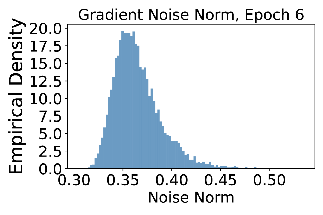
(b) Epoch 6

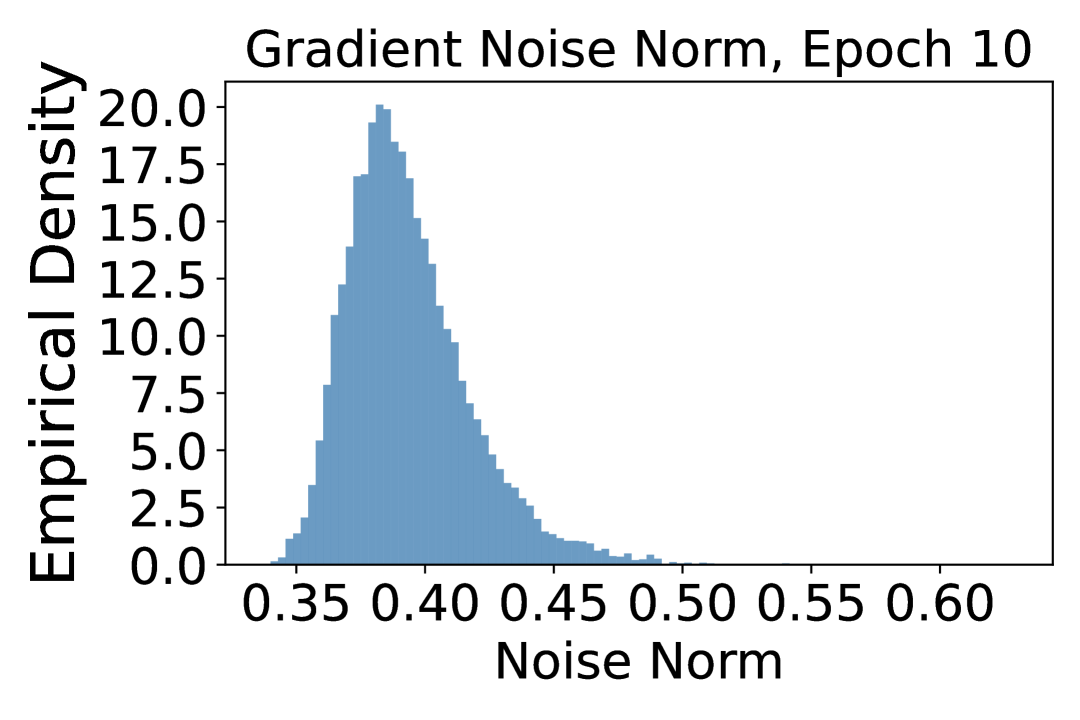
(c) Epoch 10

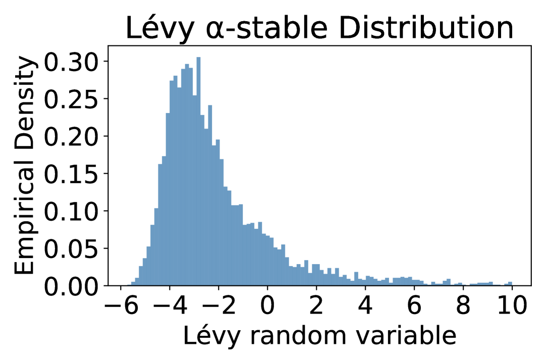
(d) $\alpha$-stable distribution

Figure 1: Comparisons of the empirical density of gradient noise norm in different epochs of training a Transformer model with a synthetic Lévy $\alpha$-stable distribution.

Remark 2 (Empirical evidence).

Similar to [17, 23], we investigate the empirical distribution of the gradient noise norm $\|\bm{g}(\bm{x},\bm{\xi})-\nabla f(\bm{x})\|$ in a centralized setting by training a GPT model [50] with 3M parameters on the Multi30k dataset [31], where $\bm{g}(\bm{x})$ denotes the mini-batch stochastic gradient and $\nabla f(\bm{x})$ denotes the full-batch gradient. We train the model for 12 epochs using SGD and plot the empirical density of the noise norm at the beginning of epochs 0, 6, and 10. As shown in Figure 1, as training progresses, the tail of the empirical gradient noise norm distribution becomes heavier (and longer) and increasingly resembles that of a synthetic $\alpha$-stable distribution.

For peer-to-peer communication in decentralized settings, we need to specify a mixing matrix $\bm{W}$ on graph $\mathcal{G}=(\mathcal{V},\mathcal{E})$.

Assumption 4 (Weight matrix).

The nonnegative weight matrix $\bm{W}$, whose $(i,r)$-th component of $\bm{W}$, denoted as $w_{ir}$, is positive if and only if $(i,r)\in E$ or $i=r$, has the following properties:

• $\bm{W}$ is primitive;

• $\bm{W}$ is doubly stochastic, i.e., $\mathbf{1}_{n}\bm{W}=\mathbf{1}_{n}$ and $\bm{W}\mathbf{1}_{n}=\mathbf{1}_{n}$.

Assumption 4 is standard in the decentralized optimization literature [51], and it guarantees that there exits some nonnegative $\lambda$, i.e., spectral gap, such that

$$\|\bm{W}-\mathbf{1}_{n}\mathbf{1}^{\top}/n\|_{2}:=\lambda<1.$$

The assumed weight matrix $\bm{W}$ can be constructed on undirected and connected graphs [52], and also on some directed and strongly connected graphs that are weight-balanced [53]. For instance, the family of directed exponential graphs, is weight-balanced and serves as an important topology configuration in decentralized training [54].

3 Algorithm Development: GT-NSGDm

We now describe the proposed Algorithm GT-NSGDm and discuss the intuition of its construction. We use $\bm{x}_{i}^{t}$ to denote the estimate of a stationary point for the global cost function $f$ at node $i$ and $t$-th iteration, and recall that $\bm{g}_{i}(\bm{x}_{i}^{t},\bm{\xi}_{i}^{t})$ denotes the corresponding stochastic gradient returned from local first-order oracle. Motivated by the error-feedback approach in [30], which serves as a momentum-type of variance reduction after applying a nonlinear operator to handle heavy-tailed noise, we also employ local momentum variance reduction

$$\bm{v}_{i}^{t}=\beta\bm{v}_{i}^{t-1}+(1-\beta)\bm{g}_{i}(\bm{x}_{i}^{t},\bm{\xi}_{i}^{t}),$$ (1)

where $\beta\in[0,1)$ serves as the momentum coefficient. Then, we use gradient tracking [12] to handle heterogeneous local functions $\{f_{i}\}_{i=1}^{n}$. Specifically, we use an estimator $\bm{y}_{i}^{t}$ to track global gradient

$$\bm{y}_{i}^{t}=\sum_{r=1}^{n}w_{ir}\big{(}\bm{y}_{r}^{t-1}+\bm{v}_{r}^{t}-\bm{v}_{r}^{t-1}\big{)}.$$ (2)

It is known that gradient tracking [12] helps eliminate the dependence on heterogeneity among local functions $\{f_{i}\}_{i=1}^{n}$, such as the requirement of bounded gradient similarity. Furthermore, similar to the approach in [27], which uses normalization to address heavy-tailed noise in centralized settings, we avoid applying normalization in the recursive updates of the local gradient estimator $\bm{v}_{i}^{t}$ in (1) and the global gradient tracker $\bm{y}_{i}^{t}$. Instead, normalization is applied only during the update of $\bm{x}_{i}^{t}$, with step size $\alpha$, and nonnegative mixing weights $\{w_{ir}\}$ that $w_{ir}>0$ only when $(i,r)\in\mathcal{E}$ or $i=r$,

$$\bm{x}_{i}^{t+1}=\sum_{r=1}^{n}w_{ir}\Big{(}\bm{x}_{r}^{t}-\alpha\frac{\bm{y}_{r}^{t}}{\|\bm{y}_{r}^{t}\|}\Big{)}.$$ (3)

We combine the local updates (1)(2)(3) on node $i\in\mathcal{V}$ and call it GT-NSGDm, Gradient Tracking based Normalized Stochastic Gradient Descent with momentum. When taking $\beta=0$, this simplifies to momentum-free gradient tracking with normalization in step 3. However, our analysis shows that GT-NSGDm performs optimal for some $\beta\in(0,1)$, making GT-NSGDm a non-trivial and optimal algorithmic design for the considered problem class. We provide a tabular description for GT-NSGDm in Algorithm 1, where all $\{\bm{x}_{i}^{0}\}$ are initialized from the same point $\bar{\bm{x}}^{0}$ for simplicity.

Algorithm 1 GT-NSGDm at each node $i$

0: $\bm{x}_{i}^{-1}=\bm{x}_{i}^{0}=\overline{\bm{x}}^{0},\bm{v}_{i}^{-1}=\bm{y}_{i}^{-1}=\mathbf{0}_{d},\alpha,\beta,\{w_{ir}\},T$.

1: for $t=0$ to $T-1$ do

2:  Sample $\bm{\xi}_{i}^{t}$; (random sample for stochastic gradient)

3:  $\bm{v}_{i}^{t}\leftarrow\beta\bm{v}_{i}^{t-1}+(1-\beta)\bm{g}_{i}(\bm{x}_{i}^{t},\bm{\xi}_{i}^{t})$; (local gradient estimator)

4:  $\bm{y}_{i}^{t}\leftarrow\sum_{r=1}^{n}w_{ir}(\bm{y}_{r}^{t-1}+\bm{v}_{r}^{t}-\bm{v}_{r}^{t-1})$; (local gradient tracker)

5:  $\bm{x}_{i}^{t+1}\leftarrow\sum_{r=1}^{n}w_{ir}\big{(}\bm{x}_{r}^{t}-\alpha\frac{\bm{y}_{r}^{t}}{\|\bm{y}_{r}^{t}\|}\big{)}$; (peer-to-peer communication)

6: end for

Remark 3 (Why vanilla gradient normalization fails?).

Although vanilla normalization is successfully used in centralized settings to robustify SGD against heavy-tailed noise [26], its direct extension to the decentralized settings fails. Suppose we run a vanilla decentralized normalized (noiseless) gradient descent, i.e., in parallel $\forall i\in\mathcal{V}$,

$$\bm{x}_{i}^{t+1}=\sum_{i=1}^{n}w_{ir}\big{(}\bm{x}_{r}^{t}-\alpha\frac{\nabla f_{r}(\bm{x}_{r}^{t})}{\|\nabla f_{r}(\bm{x}_{r}^{t})\|}\big{)}.$$ (4)

Then, the global average $\bar{\bm{x}}^{t}$ would update in the negative direction of the sum of normalized local gradients: $\bar{\bm{x}}^{t+1}=\bar{\bm{x}}^{t}-\frac{\alpha}{n}\sum_{r=1}^{n}\frac{\nabla f_{r}(\bm{x}_{r}^{t})}{\|\nabla f_{r}(\bm{x}_{r}^{t})\|}.$ Let for some $t,\forall r\in\mathcal{V},\bm{x}_{r}^{t}=\bm{x}_{*}=\mathop{\mathrm{arg\,min}}\sum_{r=1}^{n}f_{i}(\bm{x})$, i.e., all nodes hold the optimal global solution that $\sum_{r=1}^{n}\nabla f_{r}(\bm{x}_{*})=\mathbf{0}$. Since $\|\nabla f_{r}(\bm{x}_{*})\|$ can be different quantities for $r=1,\ldots,n$, due to function heterogeneity, then $\bar{\bm{x}}^{t+1}$ will move away from $\bm{x}_{*}$. Therefore, vanilla gradient normalization adds some intrinsic errors from heterogeneous local normalizations. By incorporating gradient tracking, we expect that $\bm{y}_{r}^{t}$ would converge to its global average $\bar{\bm{y}}^{t}$, and $\bar{\bm{y}}^{t}$ would converge to $(1/n)\sum_{i=r}^{n}\nabla f_{i}(\bm{x}_{r}^{t})$. In this way, $\bm{x}_{r}^{t}$ would move along the direction of the normalized sum of local gradients, and thus emulating the centralized setting.

In the following claim, we further demonstrate that vanilla gradient normalization can cause the iterates $\bm{x}_{i}^{t}$ to remain arbitrarily far from the optimal solution (see Appendix A for a proof).

Claim 1.

Consider algorithm 4. For any even $n$, for any $B\geq 1$, there exist $\{f_{i}\}_{i=1}^{n}$ satisfying Assumptions 1-2, a gradient oracle satisfying Assumption 3, a mixing matrix satisfying Assumption 4, and an initialization $\bm{x}_{0}$, such that the associated parameters $f_{*}$, $L$, $\sigma$, $\bm{W}$, $\bm{x}_{0}$, are independent of $B$. Then, $\forall T\geq 1,\forall\alpha>0$, it holds that $\frac{1}{nT}\sum_{t=0}^{T-1}\sum_{i=1}^{n}\mathbb{E}\big{[}\|\nabla f(\bm{x}_{i}^{t})\|\big{]}\geq B$.

We break the limitations of vanilla gradient normalization in Claim 1 by incorporating gradient tracking and momentum-based variance reduction. This enables the successful use of normalization to suppress heavy-tailed noise while maintaining optimal convergence despite the added nonlinearity.

4 Main Results

We present the main convergence results of GT-NSGDm  and discuss their implications. The detailed analyses are deferred to the Appendix B. We first consider the case where the tail index $p$ is known.

Theorem 1.

Let Assumptions 1, 2, 3, 4 hold. Denote $f(\bar{\bm{x}}^{0})-f_{*}=\Delta_{0},[\nabla f_{1}(\bar{\bm{x}}^{0}),\ldots,\nabla f_{n}(\bar{\bm{x}}^{0})]^{\top}=\nabla F(\mathbf{1}_{n}\otimes\bar{\bm{x}}^{0})$. Take

$$\alpha=\min\Big{(}1,\ \max\Big{(}\sqrt{\frac{\Delta_{0}(1-\beta)(1-\lambda)}{4LT}},\sqrt{\frac{\Delta_{0}(1-\lambda)}{(1+2.5L)T}},\sqrt{\frac{(1-\lambda)^{2}\Delta_{0}}{2n^{\frac{1}{2}}LT}}\Big{)}\Big{)},$$ (5)

and $1-\beta=1/T^{\frac{p}{3p-2}}$. Assume $\beta\geq 1/10$, then the sequence generated from GT-NSGDm satisfies that

$$\frac{1}{nT}\sum_{t=0}^{T-1}\sum_{i=1}^{n}\mathbb{E}\big{[}\|\nabla f(\bm{x}_{i}^{t})\|]=O\Big{(}\frac{\sigma}{n^{1-\frac{1}{p}}T^{\frac{p-1}{3p-2}}}+\frac{1}{T^{\frac{p-1}{3p-2}}}\sqrt{\frac{L\Delta_{0}}{1-\lambda}}+\frac{\|\nabla f(\bar{\bm{x}}^{0})\|}{T^{\frac{2p-2}{3p-2}}}+\sqrt{\frac{(1+2.5L)\Delta_{0}}{(1-\lambda)T}}$$

$$+\sqrt{\frac{n^{\frac{1}{2}}L\Delta_{0}}{(1-\lambda)^{2}T}}+\frac{\sigma n^{\frac{1}{2}}}{(1-\lambda)^{\frac{1}{p}}T^{\frac{p}{3p-2}}}+\frac{\|\nabla F(\mathbf{1}_{n}\otimes\bar{\bm{x}}^{0})\|}{(1-\lambda)n^{\frac{1}{2}}T^{\frac{p}{3p-2}}}+\frac{\sigma}{1-\lambda}\frac{n^{\frac{1}{2}}}{T^{\frac{2p-1}{3p-2}}}+\frac{\Delta_{0}}{T}\Big{)}.$$

Remark 4 (Order-optimal rate).

Theorem 1 establishes a non-asymptotic upper bound on the mean $\ell_{2}$ norm stationary gap of GT-NSGDm over any finite time horizon $T$. The $O(\cdot)$ here only absorbs universal constants and preserves all problem parameters. It achieves the optimal $O\big{(}1/T^{\frac{p-1}{3p-2}}\big{)}$ convergence rate in terms of $T$ as it matches the lower bound proved in [17]. This optimal guarantee is achieved in decentralized settings for the first time.

Remark 5 (Speedup in $n$).

We discuss the asymptotic speedup in number of nodes $n$. For sufficiently large $T$ (or sufficiently small target optimality gap), the upper bound in Theorem 1 is dominated by the leading terms

$$(1/T^{\frac{p-1}{3p-2}})\Big{(}\frac{\sigma}{n^{1-1/p}}+\sqrt{\frac{L\Delta_{0}}{1-\lambda}}\Big{)}.$$

In the high-noise regime $\sigma\gg n^{1-\frac{1}{p}}\sqrt{\frac{L\Delta_{0}}{1-\lambda}}$, the upper bound has a speedup factor $n^{1-\frac{1}{p}}$. In practice, the noise scale (measured by $\sigma$) in training attention models or in other high-dimensional problems can be very large, and the speedup in $n$ contributes as a noise reduction.

When the tail index $p$ is unknown in advance, we establish the following convergence rate.

Theorem 2.

Let Assumptions 1, 2, 3, 4 hold and take $\alpha$ as in (5). Take $1-\beta=1/\sqrt{T}$ and assume $\beta\geq 1/10$. Then GT-NSGDm guarantees that

$$\frac{1}{nT}\sum_{t=0}^{T-1}\sum_{i=1}^{n}\mathbb{E}\big{[}\|\nabla f(\bm{x}_{i}^{t})\|]$$

$$\leq\ O\Big{(}\frac{\sigma}{n^{1-\frac{1}{p}}}\cdot\frac{1}{T^{\frac{p-1}{2p}}}+\frac{1}{T^{\frac{1}{4}}}\sqrt{\frac{L\Delta_{0}}{1-\lambda}}+\frac{\|\nabla f(\bar{\bm{x}}^{0})\|}{\sqrt{T}}+\sqrt{\frac{(1+2.5L)\Delta_{0}}{(1-\lambda)T}}+\frac{\sigma n^{\frac{1}{2}}}{(1-\lambda)^{\frac{1}{p}}}\frac{1}{\sqrt{T}}+$$

$$\frac{\|\nabla F(\mathbf{1}_{n}\otimes\bar{\bm{x}}^{0})\|}{(1-\lambda)n^{\frac{1}{2}}}\cdot\frac{1}{\sqrt{T}}+\sqrt{\frac{n^{\frac{1}{2}}L\Delta_{0}}{(1-\lambda)^{2}T}}+\frac{\sigma n^{\frac{1}{2}}}{1-\lambda}\cdot\frac{1}{T^{\frac{2p-1}{2p}}}+\frac{\Delta_{0}}{T}\Big{)}.$$

Theorem 2 establishes an upper bound of $O(1/T^{\frac{p-1}{2p}})$ when the tail index $p$ is unknown, matching the best-known rate in the centralized setting where algorithm parameters do not rely on $p$ [27]. While the convergence rate in [30] is also independent of the knowledge of $p$, it is only for strongly convex functions and its exact rate exponent remains unspecified.

Remark 6 (Speedup in $n$ and topology independent rate).

Consider $p\in(1,2)$, i.e., the heavy-tailed case with unbounded variance this paper focuses on. When $T$ is sufficiently large (as required to achieve sufficiently small target optimality gap), the upper bound in Theorem 2 is dominated by $\frac{\sigma}{n^{1-1/p}}\cdot\frac{1}{T^{(p-1)/2p}}$. Significantly, this upper bound is independent of network topology $(\lambda)$ and exhibits a speedup factor $n^{1-1/p}$ in all regimes.

5 Experiments

We assess the performance of GT-NSGDm through numerical experiments. We first conduct empirical studies on synthetic datasets that mimic language modeling under controlled heavy-tailed noise injection, following a similar setup in [35]. We also present experimental studies on decentralized training of a small decoder-only Transformer (GPT) model with 3M parameters on the Multi30k dataset.

Baseline methods. We compare GT-NSGDm with several decentralized baseline methods: DSGD [55], DSGD-Clip [29], GT-DSGD [7], and SClip-EF-Network [30]. Among these, DSGD and GT-DSGD serve as baselines for decentralized optimization under regular stochastic noise with bounded variance. DSGD-Clip with decaying stepsize and increasing $\ell_{2}$ clipping levels, is shown to converge for strongly convex functions assuming compact domain in [56]. SClip-EF-Network achieves convergence under symmetric noise with bounded $\mathbb{E}\big{[}\|\bm{\xi}_{i}^{t}\|^{p}\mid\mathcal{F}_{t-1}\big{]}$ for $p=1$. All baseline methods are initialized from the same point. A detailed summary of these baselines is provided in Table 1 in Appendix C.1. In our experiments, all algorithms are tuned from grid search.

Network Topology. We consider the three different graph topologies: undirected ring graphs, directed exponential graphs, and complete graphs (See [6, 2, 54] for details on graph configurations). For each topology, we compute the mixing matrix using Metropolis weights [57]. In our synthetic experiments, we set the number of nodes to $n=20$, resulting in $\lambda=0.904$, $0.714$, and $0$ for the ring, exponential, and complete graphs, respectively. For decentralized training of Transformer models, we use $n=8$, with corresponding $\lambda=0.804$, $0.6$, and $0$.

5.1 Robust linear regression on synthetic tokenized data

We consider a nonconvex regularized linear regression model, on a synthetic dataset that mimics language tokens. In language modeling, token frequencies often exhibit a heavy-tailed distribution: a few tokens appear very frequently, while the vast majority are rare but contribute essential contextual meaning. We construct the following synthetic dataset $\bm{X}$ of 1k samples of dimension $d=20$. The first two features are to simulate frequent tokens, and are sampled from Bernoulli distributions Bern(0.9) and Bern(0.5), respectively. The remaining 8 features represent rare tokens and are each sample from Bern(0.1). The optimal weight vector $\bm{w}_{*}$ is sampled from a Gaussian distribution, and true label vector is $\bm{y}=\bm{X}\bm{w}_{*}$. The synthetic dataset $(\bm{X},\bm{y})$ is evenly distributed over $n=20$ nodes, where each node $i$ holds a sub-dataset $(\bm{X}_{i},\bm{y}_{i})$, estimate $\bm{w}_{i}$, and a linear regression model with nonconvex robust Tukey’s biweight loss function [58] to estimate the ground truth parameter $\bm{w}_{*}$. We inject three different zero-mean noises, Gaussian noise ($\mathcal{N}(\mathbf{0},3\bm{I}_{d})$), Student’s $t$ noise (degrees of freedom $1.5$, scale $1.0$), and Lévy $\alpha$-stable noise (stability parameter $1.5$, skewness parameter $0.5$, scale $1.0$, non-symmetric, multiplied by $0.1$) into computed exact gradient, and use corrupted stochastic gradients for algorithm updates. See Appendix C.2 for additional details.

In Figure 2, we evaluate the performance of GT-NSGDm against baseline methods on a ring graph under various types of injected gradient noise. The results show that while DSGD and GT-DSGD converge under Gaussian noise (which has bounded variance), they become unstable when exposed to heavy-tailed noise. Although DSGD-Clip remains stable across all noise types, it fails to converge to the optimum. In contrast, both GT-NSGDm and SClip-EF-Network exhibit robust convergence behavior and achieve near-optimal performance consistently across all noise scenarios. Although SClip-EF-Network outperforms GT-NSGDm by a small margin in this low-dimensional synthetic problem, GT-NSGDm outperforms it significantly in Transformers training over a real-world corpus.

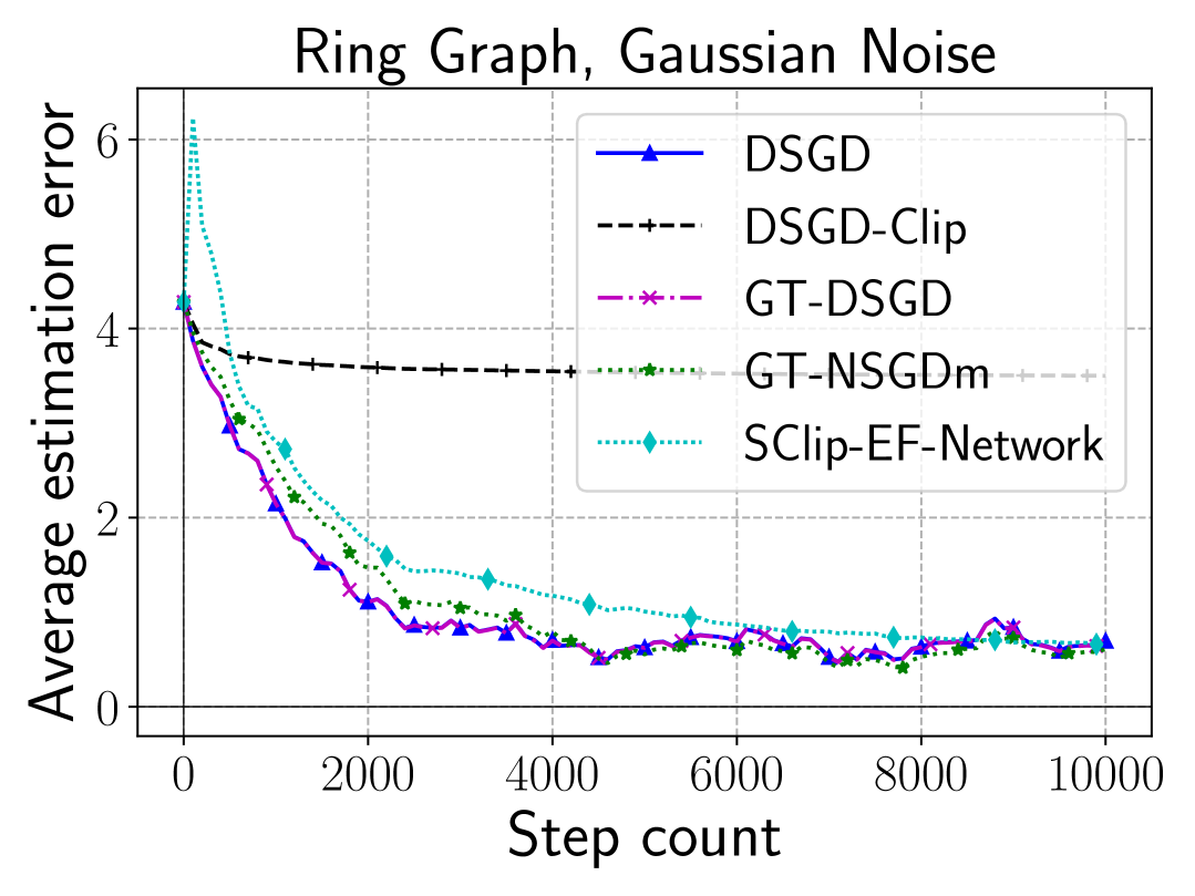
(a) Gaussian Noise

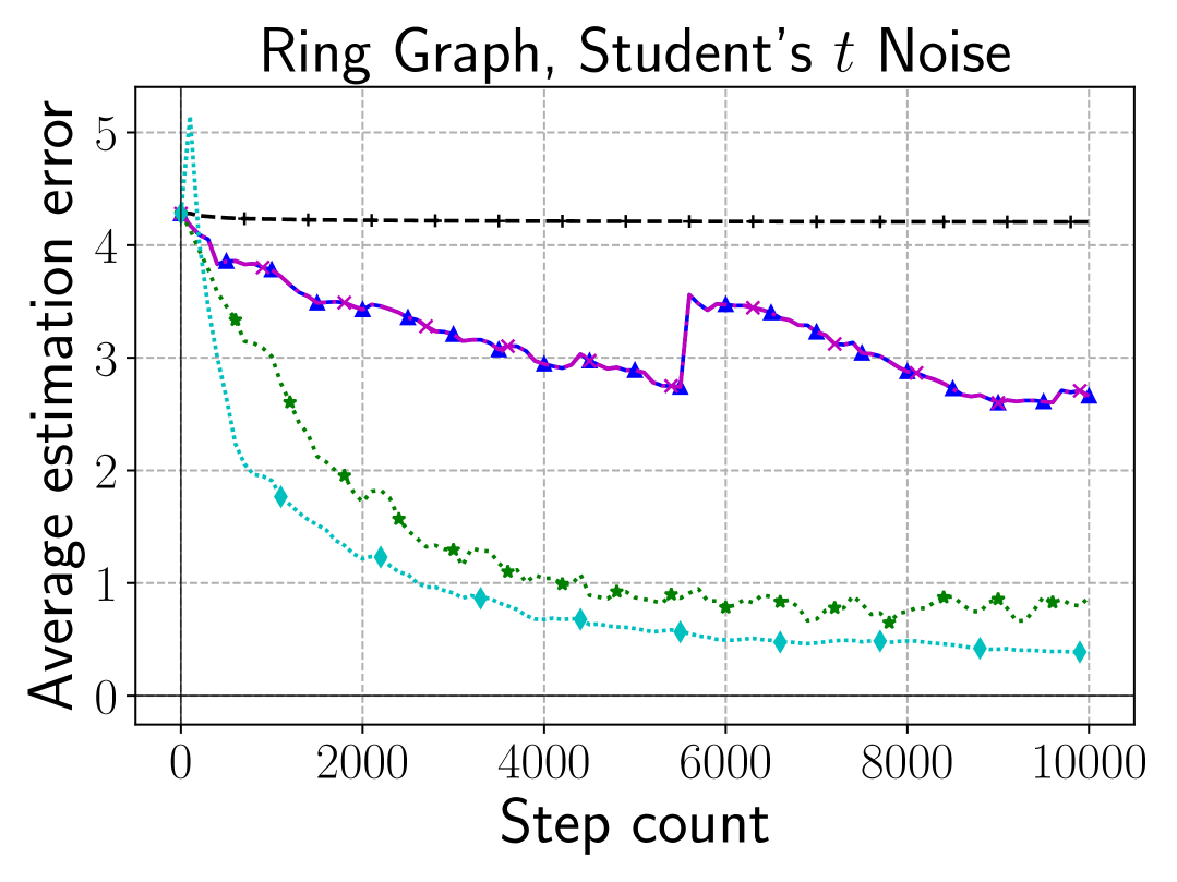
(b) Student’s $t$ noise

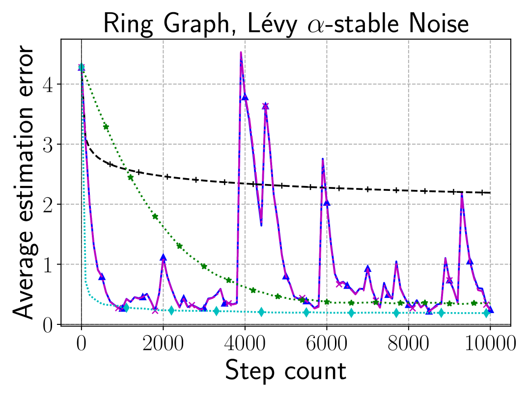
(c) Lévy $\alpha$-stable noise

Figure 2: Comparison of performance on a ring graph under various types of injected stochastic gradient noise, measured by the average estimation error $(1/n)\sum_{i=1}^{n}\|\bm{w}_{i}^{t}-\bm{w}_{*}\|$ over step count $t$.

In Figure 3, we study GT-NSGDm’s empirical dependence on problem parameters including connectivity ($\lambda$), noise level ($\sigma$), and the number of nodes ($n$). We vary each parameter while keeping the others fixed. In Figure 3(a), we inject the aforementioned Lévy $\alpha$-stable noise and test the performance of GT-NSGDm on ring, directed exponential, undirected exponential, and complete graphs with $\lambda=0.904,0.714,0.6,0$, respectively. It is shown that GT-NSGDm achieves comparable final errors under weak connectivity (i.e., large $\lambda$) comparing to complete graphs, demonstrating its favorable dependence on network connectivity under heavy-tailed noise. In Figure 3(b), we evaluate GT-NSGDm’s performance under different noise levels on a directed exponential graph. Under Gaussian noise with scale 1 (unit variance), GT-NSGDm reaches the best optimality; the final error increases as $\sigma$ grows, as observed under both Gaussian and Lévy $\alpha$-stable noise. In Figure 3(c), we inject Lévy $\alpha$-stable noise and use complete graphs ($\lambda=0$ for all $n$) with varying number of nodes. we observe that as $n$ increases from 2 to 40, convergence speed improves. The corresponding final errors, i.e., $[0.4,0.35,0.29,0.20,0.21]$, demonstrate a clear speedup trend over a certain range of $n$, supporting the theoretical speedup discussions in Remarks 5 and 6.

(a) Dependence on $\lambda$

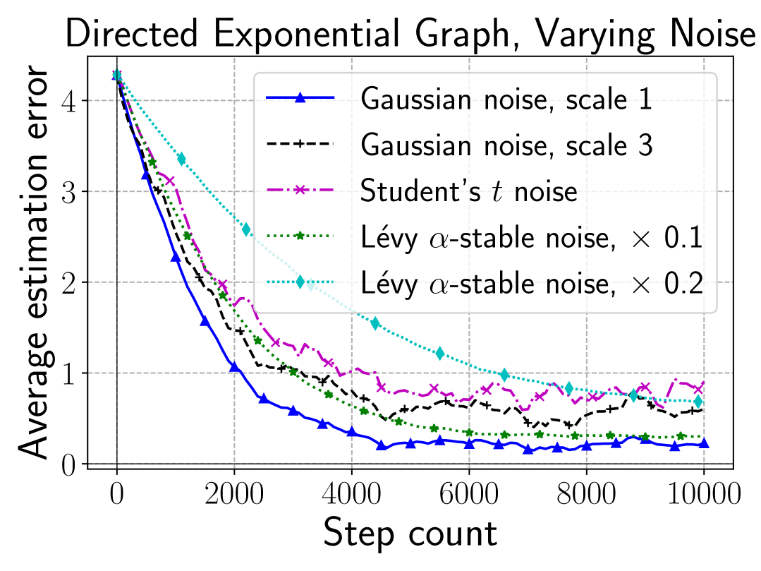
(b) Dependence on $\sigma$

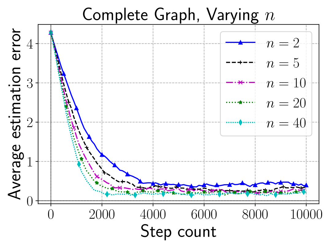
(c) Dependence on $n$

Figure 3: Empirical studies on GT-NSGDm’s dependence on problem parameters $\lambda,\sigma,n$.

5.2 Decentralized training of Transformers

We further evaluate GT-NSGDm on real-world language modeling tasks. Specifically, we consider a GPT model [50] with approximately 3 million parameters and perform an auto-regressive language modeling task on the Multi30k dataset (29,000 sentences and 4.4 million tokens in the training split). We assess algorithm performance using validation logarithmic perplexity. On a graph of 8 nodes (with the three topologies), we evenly distribute the training corpus across the nodes and initialize an identical GPT model on each. We run GT-NSGDm and baseline methods for 12 epochs with a batch size of 64. See Appendix C.3 for additional details on model and hyperparameter search.

In Figure 4, we plot the average validation loss and its standard deviation over five independent runs for each algorithm across three different topologies. The results show that, in this high-dimensional real-world task, GT-NSGDm is the only algorithm that consistently converges to near-zero loss with low variance, achieving average final loss levels of 0.258, 0.261, and 0.282 on ring, directed exponential, and complete graphs, respectively. Other baseline methods, while stable, plateau at loss levels between 5 and 6. This sharp contrast underscores that GT-NSGDm is not only theoretically sound but also robust in real-world tasks.

(a) Ring Graph

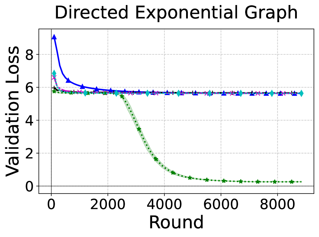
(b) Directed Exponential Graph

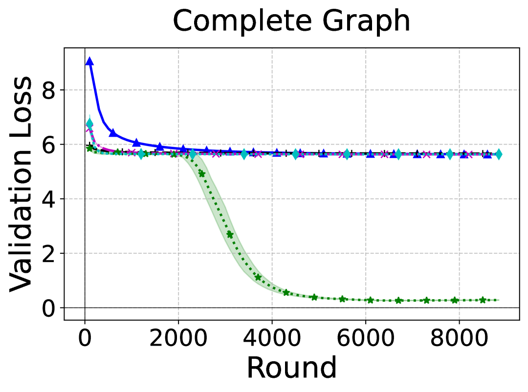
(c) Complete Graph

Figure 4: Comparison of graph-wide average validation losses in decentralized training of Transformer models, over ring, directed exponential, and complete graphs.

6 Conclusion and Future Work

In this paper, we have proposed GT-NSGDm for solving decentralized nonconvex smooth optimization to address heavy-tailed noise. The key idea is to leverage normalization, together with momentum variance reduction, to combat heavy-tailed noise, and use gradient tracking to handle cross-node heterogeneity and the nonlinearity brought by normalization. Theoretical analyses establish that GT-NSGDm attains optimal convergence rate when the tail index $p$ is known, and a rate that matches the best centralized one when $p$ is unknown. Extensive experiments on nonconvex linear regression and decentralized Transformer training show that GT-NSGDm is robust and efficient under heavy-tailed noise across various topologies, and achieves a speedup in $n$. Future directions include extending the current analysis to other nonlinearities, such as sign and clipping [17], and generalizing GT-NSGDm to handle objective functions under relaxed smoothness conditions [27].

Appendix

Appendix A Proof of Claim 1

Proof.

Consider $n$ scalar functions that for each $i\in\mathcal{V}$, $f_{i}(x)=(1/2)(x-a_{i})^{2}$ for some $a_{i}$, and complete graph with $\bm{W}=(1/n)\mathbf{1}_{n}\mathbf{1}_{n}^{\top}$. Let $a_{i}=a,\forall i=1,\ldots,n/2$, and $a_{i}=b,\forall i=n/2+1,\ldots,n$, and $b-a>2B+1$. Let $x_{i}^{0}=a+0.5,\forall i\in\mathcal{V}$. Then, $\forall i\in\mathcal{V}$, vanilla normalization reduces to

$$x_{i}^{1} =\frac{1}{n}\sum_{r=1}^{n}\Big{(}x_{r}^{0}-\alpha\text{sign}(x_{r}^{0}-a_{r})\Big{)}$$

$$=x_{r}^{0}-\frac{\alpha}{n}\sum_{r=1}^{n}\text{sign}(x_{r}^{0}-a_{r})$$

$$=x_{r}^{0}-\frac{\alpha}{n}\sum_{r=1}^{n/2}\text{sign}(0.5)-\frac{\alpha}{n}\sum_{r=n/2+1}^{n}\text{sign}(0.5-(b-a))$$

$$=x_{r}^{0}.$$

Therefore, $x_{r}^{t}=a+0.5,\forall r\in\mathcal{V},\forall t\geq 0$. Since the optimal solution to the original problem is $\frac{a+b}{2}$, the optimality gap is $\frac{b-a}{2}-0.5\geq B$. ∎

Remark 7.

Note that the proof above can be further extended to the case where the gradient oracle admits almost surely bounded gradient noise. We can use the noise bound to adapt the choices of $a,b,\varepsilon$ such that all signs still get canceled.

Appendix B Proofs of Theorems

B.1 Preliminaries

We define some stacked long vectors,

$$F(\bm{x}^{t}) :=[f_{1}(\bm{x}_{1}^{t}),\ldots,f_{n}(\bm{x}_{n}^{t})]^{\top},$$

$$\nabla F(\bm{x}^{t}) :=[\nabla f_{1}(\bm{x}_{1}^{t})^{\top},\ldots,\nabla f_{n}(\bm{x}_{n}^{t})^{\top}]^{\top},$$

$$\bm{g}(\bm{x}^{t},\bm{\xi}^{t}) :=[\bm{g}_{1}(\bm{x}_{1}^{t},\bm{\xi}_{1}^{t})^{\top},\ldots,\bm{g}_{n}(\bm{x}_{n}^{t},\bm{\xi}_{n}^{t})^{\top}]^{\top}$$

$$\bm{v}^{t} :=[(\bm{v}_{1}^{t})^{\top},\ldots,(\bm{v}_{n}^{t})^{\top}]^{\top},$$

$$\mathcal{N}(\bm{y}^{t}) :=\Big{[}\frac{(\bm{y}_{1}^{t})^{\top}}{\|\bm{y}_{1}^{t}\|},\ldots,\frac{(\bm{y}_{n}^{t})^{\top}}{\|\bm{y}_{n}^{t}\|}\Big{]}^{\top},$$

$$\bm{x}^{t} :=[(\bm{x}_{1}^{t})^{\top},\ldots,(\bm{x}_{n}^{t})^{\top}]^{\top}.$$

Then, Algorithm 1 can be rewritten in the compact long-vector form:

$$\bm{v}^{t} =\beta\bm{v}^{t-1}+(1-\beta)\bm{g}(\bm{x}^{t},\bm{\xi}^{t});$$ (6)

$$\bm{y}^{t} =\big{(}\bm{W}\otimes\bm{I}_{d}\big{)}(\bm{y}^{t-1}+\bm{v}^{t}-\bm{v}^{t-1}),$$ (7)

$$\bm{x}^{t+1} =\big{(}\bm{W}\otimes\bm{I}_{d}\big{)}(\bm{x}^{t}-\alpha\mathcal{N}(\bm{y}^{t})).$$ (8)

We define the following averages over network:

$$\bar{\bm{v}}^{t}=\frac{1}{n}\sum_{i=1}^{n}\bm{v}_{i}^{t},\quad\bar{\bm{y}}^{t}=\frac{1}{n}\sum_{i=1}^{n}\bm{y}_{i}^{t},\quad\tilde{\bm{y}}^{t}=\frac{1}{n}\sum_{i=1}^{n}\frac{\bm{y}_{i}^{t}}{\|\bm{y}_{i}^{t}\|},\quad\bar{\bm{x}}^{t}=\frac{1}{n}\sum_{i=1}^{n}\bm{x}_{i}^{t},\quad\overline{\nabla}F(\bm{x}^{t})=\frac{1}{n}\sum_{i=1}^{n}\nabla f_{i}(\bm{x}_{i}^{t}).$$ (9)

From the doubly stochasticity of $\bm{W}$, the global average updates as

$$\bar{\bm{x}}^{t+1}=\bar{\bm{x}}^{t}-\frac{\alpha}{n}\sum_{r=1}^{n}\frac{\bm{y}_{r}^{t}}{\|\bm{y}_{r}^{t}\|}=\bar{\bm{x}}^{t}-\alpha\tilde{\bm{y}}^{t}.$$ (10)

B.2 Intermediate Lemmas

We first present some standard useful relations to be used in our analyses.

Lemma 1.

The following relations hold:

1. $\bar{\bm{y}}^{t}=\bar{\bm{v}}^{t}$;

2. $\bm{W}-\mathbf{1}_{n}\mathbf{1}_{n}^{\top}/n=(\bm{W}-\mathbf{1}_{n}\mathbf{1}_{n}^{\top}/n)(\bm{I}_{n}-\mathbf{1}_{n}\mathbf{1}_{n}^{\top}/n)=(\bm{I}_{n}-\mathbf{1}_{n}\mathbf{1}_{n}^{\top}/n)(\bm{W}-\mathbf{1}_{n}\mathbf{1}_{n}^{\top}/n)$;

3. $\bm{W}^{k}-\mathbf{1}_{n}\mathbf{1}_{n}^{\top}/n=(\bm{W}-\mathbf{1}_{n}\mathbf{1}_{n}^{\top}/n)^{k},\forall k\in\mathbb{N}_{+}$;

4. $(1/\sqrt{n})\sum_{i=1}^{n}\|\bm{a}_{i}\|\leq\|\bm{a}\|\leq\sum_{i=1}^{n}\|\bm{a}_{i}\|$, $\forall\bm{a}=[\bm{a}_{1}^{\top},\ldots,\bm{a}_{n}^{\top}]^{\top}\in\mathbb{R}^{nd}$,

5. $\sum_{i=1}^{m}a_{i}^{p}\leq\big{(}\sum_{i=1}^{m}a_{i}\big{)}^{p}\leq m^{p-1}\sum_{i=1}^{m}a_{i}^{p},\forall m\in\mathbb{N}_{+},\forall a_{i}\in\mathbb{R}_{+}$.

We then present a standard decent lemma for $L$-smooth functions .

Lemma 2 (Decent lemma for $L$-smooth functions).

Let Assumption 2 hold. For any $\bm{x},\bm{y}\in\mathbb{R}^{d}$, there holds

$$f(\bm{y})\leq f(\bm{x})+\nabla f(\bm{x})^{\top}(\bm{y}-\bm{x})+\frac{L}{2}\|\bm{x}-\bm{y}\|^{2}.$$

We next present the main descent lemma on the network average.

Lemma 3 (Decent lemma for network average).

Let Assumption 2 hold. Let $\bm{\epsilon}^{t}=\bar{\bm{y}}^{t}-\nabla f(\bar{\bm{x}}^{t})$. We have

$$\sum_{t=0}^{T-1}\alpha\|\nabla f(\bar{\bm{x}}^{t})\|\leq f(\bar{\bm{x}}^{0})-f_{*}+\sum_{t=0}^{T-1}2\alpha\|\bm{\epsilon}^{t}\|+\sum_{t=0}^{T-1}\frac{\alpha}{n}\sum_{i=1}^{n}\|\bar{\bm{y}}^{t}-\bm{y}_{i}^{t}\|+\sum_{t=0}^{T-1}\frac{L}{2}\alpha^{2}.$$

Proof.

Since $\|\bar{\bm{x}}^{t+1}-\bar{\bm{x}}^{t}\|=\alpha\|\tilde{\bm{y}}^{t}\|=\alpha$, applying Lemma 2 on $\bar{\bm{x}}^{t+1},\bar{\bm{x}}^{t}$ gives that

$$f(\bar{\bm{x}}^{t+1}) \leq f(\bar{\bm{x}}^{t})+\nabla f(\bar{\bm{x}}^{t})^{\top}(\bar{\bm{x}}^{t+1}-\bar{\bm{x}}^{t})+\frac{L}{2}\|\bar{\bm{x}}^{t+1}-\bar{\bm{x}}^{t}\|^{2}$$

$$\overset{(i)}{\leq}f(\bar{\bm{x}}^{t})-\alpha(\bar{\bm{y}}^{t}-\bm{\epsilon}^{t})^{\top}\tilde{\bm{y}}^{t}+\frac{L}{2}\alpha^{2}$$

$$\overset{(ii)}{\leq}f(\bar{\bm{x}}^{t})-\alpha(\bar{\bm{y}}^{t})^{\top}\tilde{\bm{y}}^{t}+\alpha\|\bm{\epsilon}^{t}\|+\frac{L}{2}\alpha^{2},$$ (11)

where we used the definitions (9)(10) in $(i)$, and used Cauchy-Schwartz inequality followed by $\|\tilde{\bm{y}}^{t}\|\leq 1$ in $(ii).$ Next,

$$-(\bar{\bm{y}}^{t})^{\top}\tilde{\bm{y}}^{t} =-(\bar{\bm{y}}^{t})^{\top}\Big{[}\frac{\bar{\bm{y}}^{t}}{\|\bar{\bm{y}}^{t}\|}+\frac{1}{n}\sum_{i=1}^{n}\bm{y}_{i}^{t}\big{(}\frac{1}{\|\bm{y}_{i}^{t}\|}-\frac{1}{\|\bar{\bm{y}}^{t}\|}\big{)}\Big{]}$$

$$\leq-\|\bar{\bm{y}}^{t}\|+\|\frac{1}{n}\sum_{i=1}^{n}\bm{y}_{i}^{t}\big{(}\frac{\|\bar{\bm{y}}^{t}\|}{\|\bm{y}_{i}^{t}\|}-1\big{)}\|$$

$$\overset{(i)}{\leq}-\|\nabla f(\bar{\bm{x}}^{t})\|+\|\bm{\epsilon}^{t}\|+\frac{1}{n}\sum_{i=1}^{n}\big{|}\|\bar{\bm{y}}^{t}\|-\|\bm{y}_{i}^{t}\|\big{|}$$

$$\overset{(ii)}{\leq}-\|\nabla f(\bar{\bm{x}}^{t})\|+\|\bm{\epsilon}^{t}\|+\frac{1}{n}\sum_{i=1}^{n}\|\bar{\bm{y}}^{t}-\bm{y}_{i}^{t}\|,$$ (12)

where we used $\|\bar{\bm{y}}^{t}\|=\|\nabla f(\bar{\bm{x}}^{t})+\bm{\epsilon}^{t}\|\geq\|\nabla f(\bar{\bm{x}}^{t})\|-\|\bm{\epsilon}^{t}\|$, and Cauchy-Schwartz inequality in $(i)$, and $|\|\bm{a}\|-\|\bm{b}\||\leq\|\bm{a}-\bm{b}\|$ for any $\bm{a},\bm{b}\in\mathbb{R}^{d}$ in $(ii)$. Plugging in (12) into (11), and summing over $t=0,\ldots,T-1$, we have

$$f(\bar{\bm{x}}^{T})\leq f(\bar{\bm{x}}^{0})-\sum_{t=0}^{T-1}\alpha\|\nabla f(\bar{\bm{x}}^{t})\|+\sum_{t=0}^{T-1}2\alpha\|\bm{\epsilon}^{t}\|+\sum_{t=0}^{T-1}\frac{\alpha}{n}\sum_{i=1}^{n}\|\bar{\bm{y}}^{t}-\bm{y}_{i}^{t}\|+\sum_{t=0}^{T-1}\frac{L}{2}\alpha^{2}.$$

Using $f(\bar{\bm{x}}^{T})\geq f_{*}$ and rearranging terms above give the desired result. ∎

With Lemma 3, it remains to bound the gradient estimation error $\|\bm{\epsilon}^{t}\|$ and the consensus error $\bm{y}_{i}^{t}-\bar{\bm{y}}^{t}$. Let us decompose the gradient estimation error as follows:

$$\bm{\epsilon}^{t}=\bar{\bm{y}}^{t}-\nabla f(\bar{\bm{x}}^{t})=\bar{\bm{v}}^{t}-\nabla f(\bar{\bm{x}}^{t})=\underbrace{\bar{\bm{v}}^{t}-\overline{\nabla}F(\bm{x}^{t})}_{:=\bm{\epsilon}_{1}^{t}\in\mathbb{R}^{d}}+\underbrace{\overline{\nabla}F(\bm{x}^{t})-\nabla f(\bar{\bm{x}}^{t})}_{:=\bm{\epsilon}_{2}^{t}\in\mathbb{R}^{d}}.$$ (13)

It is clear that $\bm{\epsilon}_{1}^{t}$ is the gradient estimation error, and $\bm{\epsilon}_{2}^{t}$, exploiting the smoothness property in 2, can be bounded by the consensus error $\bm{x}_{i}^{t}-\bar{\bm{x}}^{t}$. Since the consensus error is also used in bounding $\bm{\epsilon}_{1}^{t}$, we need to first bound the consensus errors $\bm{x}_{i}^{t}-\bar{\bm{x}}^{t}$ and $\bm{y}_{i}^{t}-\bar{\bm{y}}^{t}$.

Lemma 4 (Consensus errors of $\{\bm{x}_{i}^{t}\}$).

We have for all $t=0,\ldots,T$,

$$\frac{1}{n}\sum_{i=1}^{n}\|\bm{x}_{i}^{t}-\bar{\bm{x}}^{t}\| \leq\frac{\alpha\lambda}{1-\lambda}.$$ (14)

Proof.

Using the relation 4 in Lemma 1 we have

$$\frac{1}{n}\sum_{i=1}^{n}\|\bm{x}_{i}^{t}-\bar{\bm{x}}^{t}\|\leq\frac{1}{\sqrt{n}}\|\bm{x}^{t}-\mathbf{1}_{n}\otimes\bar{\bm{x}}^{t}\|.$$ (15)

From the compact form update in (8), we have

$$\bm{x}^{t}=\big{(}\bm{W}\otimes\bm{I}_{d}\big{)}\bm{x}^{0}-\alpha\sum_{k=0}^{t-1}(\bm{W}\otimes\bm{I}_{d})^{t-k}\mathcal{N}(\bm{y}^{k}).$$

It follows that

$$\|\bm{x}^{t}-\mathbf{1}_{n}\otimes\bar{\bm{x}}^{t}\|$$

$$=\ \|\big{(}\bm{I}_{nd}-\frac{1}{n}\mathbf{1}_{n}\mathbf{1}_{n}^{\top}\otimes\bm{I}_{d}\big{)}\bm{x}^{t}\|$$

$$\overset{(i)}{=}\ \alpha\|\sum_{k=0}^{t-1}\big{(}\bm{I}_{nd}-\frac{1}{n}\mathbf{1}_{n}\mathbf{1}_{n}^{\top}\otimes\bm{I}_{d}\big{)}\big{(}\bm{W}\otimes\bm{I}_{d}\big{)}^{t-k}\mathcal{N}(\bm{y}^{k})\|$$

$$\leq\ \alpha\|\sum_{k=0}^{t-1}\|\bm{W}^{t-k}-\frac{1}{n}\mathbf{1}_{n}\mathbf{1}_{n}^{\top}\|_{2}\|\mathcal{N}(\bm{y}^{k})\|$$

$$\overset{(ii)}{\leq}\ \alpha\|\sum_{k=0}^{t-1}\|\bm{W}-\frac{1}{n}\mathbf{1}_{n}\mathbf{1}_{n}^{\top}\|_{2}^{t-k}\|\mathcal{N}(\bm{y}^{k})\|$$

$$\leq\ \alpha\sqrt{n}\sum_{k=0}^{t-1}\lambda^{t-k}$$ (16)

$$\overset{(iii)}{\leq}\ \frac{\alpha\sqrt{n}\lambda}{1-\lambda}.$$ (17)

where we used the double stochasticity of $\bm{W}$ and $\bm{x}_{i}^{0}=\bar{\bm{x}}^{0},\forall i\in[n]$ in $(i)$, the relation 3 in Lemma 1 in $(ii)$, and Assumption 4 in $(iii)$. Substituting (17) into (15) gives the desired bound in (14). ∎

Before proceeding to bound consensus errors for $\{\bm{y}_{i}^{t}\}$, we present the following bound on vector-valued martingale difference sequence from [27].

Lemma 5.

Given a sequence of random vectors $\bm{d}_{t}\in\mathbb{R}^{d}$, $\forall t$ such that $\mathbb{E}[\bm{d}_{t}\mid\mathcal{F}_{t-1}]=\mathbf{0}$ where $\mathcal{F}_{t}=\sigma(\bm{d}_{1},\ldots,\bm{d}_{t})$ is the natural filtration, then for any $p\in[1,2]$, there is

$$\mathbb{E}\Big{[}\|\sum_{t=1}^{T}\bm{d}_{t}\|\Big{]}\leq 2\sqrt{2}\mathbb{E}\Big{[}\Big{(}\sum_{t=1}^{T}\|\bm{d}_{t}\|^{p}\Big{)}^{\frac{1}{p}}\Big{]},\forall T\geq 0.$$

Lemma 6 (Consensus errors for $\{\bm{y}_{i}^{t}\}$).

We have for all $t=0,\ldots,T$,

$$\frac{1}{n}\mathbb{E}\big{[}\sum_{i=1}^{n}\|\bm{y}_{i}^{t}-\bar{\bm{y}}^{t}\|\big{]}$$

$$\leq\ 2\sqrt{2}n^{\frac{1}{2}}\big{(}\frac{1}{\beta}-1\big{)}\Big{(}\sum_{k=0}^{t}\lambda^{(t-k+1)p}\Big{)}^{\frac{1}{p}}\sigma+\frac{1}{\sqrt{n}}\big{(}\frac{1}{\beta}-1\big{)}\sum_{k=0}^{t}\lambda^{t-k+1}\mathbb{E}\big{[}\|\nabla F(\bm{x}^{k})-\bm{v}^{k}\|\big{]}.$$

Proof.

Similar to (15), we have

$$\frac{1}{n}\sum_{i=1}^{n}\|\bm{y}_{i}^{t}-\bar{\bm{y}}^{t}\|\leq\frac{1}{\sqrt{n}}\|\bm{y}^{t}-\mathbf{1}_{n}\otimes\bar{\bm{y}}^{t}\|.$$ (18)

Following from (7),

$$\bm{y}^{t}-\mathbf{1}_{n}\otimes\bar{\bm{y}}^{t}$$ (19)

$$\overset{\eqref{eq:compact-update-y}}{=}\ \big{(}\bm{I}_{nd}-\frac{1}{n}\mathbf{1}_{n}\mathbf{1}_{n}^{\top}\otimes\bm{I}_{d}\big{)}\big{(}\bm{W}\otimes\bm{I}_{d}\big{)}(\bm{y}^{t-1}+\bm{v}^{t}-\bm{v}^{t-1})$$

$$=\ \big{(}\bm{W}\otimes\bm{I}_{d}-\frac{1}{n}\mathbf{1}_{n}\mathbf{1}_{n}^{\top}\otimes\bm{I}_{d}\big{)}\bm{y}^{t-1}+\big{(}\bm{W}\otimes\bm{I}_{d}-\frac{1}{n}\mathbf{1}_{n}\mathbf{1}_{n}^{\top}\otimes\bm{I}_{d}\big{)}(\bm{v}^{t}-\bm{v}^{t-1})$$

$$\overset{(i)}{=}\ \big{(}\bm{W}\otimes\bm{I}_{d}-\frac{1}{n}\mathbf{1}_{n}\mathbf{1}_{n}^{\top}\otimes\bm{I}_{d}\big{)}\big{(}\bm{I}_{nd}-\frac{1}{n}\mathbf{1}_{n}\mathbf{1}_{n}^{\top}\otimes\bm{I}_{d}\big{)}\bm{y}^{t-1}+\big{(}\bm{W}\otimes\bm{I}_{d}-\frac{1}{n}\mathbf{1}_{n}\mathbf{1}_{n}^{\top}\otimes\bm{I}_{d}\big{)}(\bm{v}^{t}-\bm{v}^{t-1})$$

$$\overset{(ii)}{=}\ \sum_{k=0}^{t}\big{(}\bm{W}\otimes\bm{I}_{d}-\frac{1}{n}\mathbf{1}_{n}\mathbf{1}_{n}^{\top}\otimes\bm{I}_{d}\big{)}^{t-k+1}(\bm{v}^{t}-\bm{v}^{t-1}),$$ (20)

where we used relation 3 in Lemma 1 in $(i)$ and used $\bm{y}_{i}^{0}=\mathbf{0}_{d},\forall i\in[n]$ in $(ii)$. From the update in (6), we have

$$\bm{v}^{t}-\bm{v}^{t-1}=(\beta-1)\bm{v}^{t-1}+(1-\beta)\bm{g}(\bm{x}^{t},\bm{\xi}^{t})=(1-\beta)(\bm{v}^{t}-\bm{v}^{t-1})+(1-\beta)(\bm{g}(\bm{x}^{t},\bm{\xi}^{t})-\bm{v}^{t}).$$

Then, there holds,

$$\bm{v}^{t}-\bm{v}^{t-1}=(\frac{1}{\beta}-1)(\bm{g}(\bm{x}^{t},\bm{\xi}^{t})-\bm{v}^{t})=(\frac{1}{\beta}-1)(\bm{g}(\bm{x}^{t},\bm{\xi}^{t})-\nabla F(\bm{x}^{k})+\nabla F(\bm{x}^{k})-\bm{v}^{t}).$$ (21)

Putting the relation above into (20) and applying (20) recursively, from $\bm{y}_{i}^{0}=\bar{\bm{y}}^{0}$, we have

$$\begin{split}\|\bm{y}^{t}-\mathbf{1}_{n}\otimes\bar{\bm{y}}^{t}\|&\leq(\frac{1}{\beta}-1)\|\sum_{k=0}^{t}\big{(}\bm{W}\otimes\bm{I}_{d}-\frac{1}{n}\mathbf{1}_{n}\mathbf{1}_{n}^{\top}\otimes\bm{I}_{d}\big{)}^{t-k+1}\big{(}\bm{g}(\bm{x}^{k},\bm{\xi}^{k})-\nabla F(\bm{x}^{k})\big{)}\|\\ &\quad+(\frac{1}{\beta}-1)\|\sum_{k=0}^{t}\big{(}\bm{W}\otimes\bm{I}_{d}-\frac{1}{n}\mathbf{1}_{n}\mathbf{1}_{n}^{\top}\otimes\bm{I}_{d}\big{)}^{t-k+1}\big{(}\nabla F(\bm{x}^{k})-\bm{v}^{k}\big{)}\|\end{split}$$ (22)

We note that the first half of the right hand side above can be addressed by Lemma 5.

$$\mathbb{E}\Big{[}\|\sum_{k=0}^{t}\big{(}\bm{W}\otimes\bm{I}_{d}-\frac{1}{n}\mathbf{1}_{n}\mathbf{1}_{n}^{\top}\otimes\bm{I}_{d}\big{)}^{t-k+1}\big{(}\bm{g}(\bm{x}^{k},\bm{\xi}^{k})-\nabla F(\bm{x}^{k})\big{)}\|\mid\mathcal{F}_{t-1}\Big{]}$$

$$\leq\ 2\sqrt{2}\mathbb{E}\Big{[}\Big{(}\sum_{k=0}^{t}\lambda^{(t-k+1)p}\|\bm{g}(\bm{x}^{k},\bm{\xi}^{k})-\nabla F(\bm{x}^{k})\|^{p}\Big{)}^{\frac{1}{p}}\mid\mathcal{F}_{t-1}\Big{]}$$

$$\leq\ 2\sqrt{2}\mathbb{E}\Big{[}\Big{(}\sum_{k=0}^{t}\lambda^{(t-k+1)p}\big{(}\sum_{i=1}^{n}\|\bm{g}_{i}(\bm{x}_{i}^{k},\bm{\xi}_{i}^{k})-\nabla f_{i}(\bm{x}_{i}^{k})\|\big{)}^{p}\Big{)}^{\frac{1}{p}}\mid\mathcal{F}_{t-1}\Big{]}$$

$$\overset{(i)}{\leq}\ 2\sqrt{2}\mathbb{E}\Big{[}\Big{(}\sum_{k=0}^{t}\sum_{i=1}^{n}\lambda^{(t-k+1)p}n^{p-1}\|\bm{g}_{i}(\bm{x}_{i}^{k},\bm{\xi}_{i}^{k})-\nabla f_{i}(\bm{x}_{i}^{k})\|^{p}\Big{)}^{\frac{1}{p}}\mid\mathcal{F}_{t-1}\Big{]}$$

$$\overset{(ii)}{\leq}\ 2\sqrt{2}\Big{(}\mathbb{E}\big{[}\sum_{i=1}^{n}\lambda^{p}n^{p-1}\|\bm{g}_{i}(\bm{x}_{i}^{t},\bm{\xi}_{i}^{k})-\nabla f_{i}(\bm{x}_{i}^{t})\|^{p}\mid\mathcal{F}_{t-1}\big{]}$$

$$\quad+\sum_{k=0}^{t-1}\sum_{i=1}^{n}\lambda^{(t-k+1)p}n^{p-1}\|\bm{g}_{i}(\bm{x}_{i}^{k},\bm{\xi}_{i}^{k})-\nabla f_{i}(\bm{x}^{k})\|^{p}\Big{)}^{\frac{1}{p}}$$

$$\overset{(iii)}{\leq}\ 2\sqrt{2}\Big{(}\lambda^{p}n^{p}\sigma^{p}+\sum_{k=0}^{t-1}\sum_{i=1}^{n}\lambda^{(t-k+1)p}n^{p-1}\|\bm{g}_{i}(\bm{x}_{i}^{k},\bm{\xi}_{i}^{k})-\nabla f_{i}(\bm{x}_{i}^{k})\|^{p}\Big{)}^{\frac{1}{p}},$$

where we used relation $5$ from Lemma 1 in $(i)$, Jensen’s inequality in $(ii)$, and Assumption 3 in $(iii)$. Applying the above arguments recursively from $\mathcal{F}_{t-2}$ to $\mathcal{F}_{0}$, we have

$$\mathbb{E}\Big{[}\|\sum_{k=0}^{t}\big{(}\bm{W}\otimes\bm{I}_{d}-\frac{1}{n}\mathbf{1}_{n}\mathbf{1}_{n}^{\top}\otimes\bm{I}_{d}\big{)}^{t-k+1}\big{(}\bm{g}(\bm{x}^{k},\bm{\xi}^{k})-\nabla F(\bm{x}^{k})\big{)}\|\Big{]}\leq 2\sqrt{2}\Big{(}\sum_{k=0}^{t}\lambda^{(t-k+1)p}\Big{)}^{\frac{1}{p}}n\sigma.$$

Therefore, using the relation above, and (18), (22), we reach the desired relation. ∎

We then bound average gradient estimation errors $\bm{\epsilon}_{1}^{t}=\bar{\bm{v}}^{t}-\overline{\nabla}F(\bm{x}^{t})$.

Lemma 7 (Average gradient estimation errors).

For all $t=0,\ldots,T$, we have

$$\mathbb{E}\big{[}\|\bar{\bm{v}}^{t}-\overline{\nabla}F(\bm{x}^{t})\|\big{]}\leq\beta^{t+1}\|\nabla f(\bar{\bm{x}}^{0})\|+\frac{2\sqrt{2}}{n^{1-\frac{1}{p}}}\Big{(}\sum_{k=0}^{t}\beta^{(t-k)p}(1-\beta)^{p}\Big{)}^{\frac{1}{p}}\sigma+\sum_{k=0}^{t}\beta^{t-k+1}\Big{(}\frac{2\alpha\lambda}{1-\lambda}+\alpha\Big{)}L.$$

Proof.

Following from the step 4 in Algorithm 1, $\forall i\in[n]$,

$$\bm{v}_{i}^{t}-\nabla f_{i}(\bm{x}_{i}^{t}) =\beta(\bm{v}_{i}^{t-1}-\nabla f_{i}(\bm{x}_{i}^{t-1}))+(1-\beta)(\bm{g}_{i}(\bm{x}_{i}^{t},\bm{\xi}_{i}^{t})-\nabla f_{i}(\bm{x}_{i}^{t}))+\beta(\nabla f_{i}(\bm{x}_{i}^{t-1})-\nabla f_{i}(\bm{x}_{i}^{t})).$$ (23)

Averaging the above relation over $i=1,\ldots,n$ leads to that:

$$\bm{\epsilon}_{1}^{t} =\bar{\bm{v}}^{t}-\overline{\nabla}F(\bm{x}^{t})$$

$$=\beta(\bar{\bm{v}}^{t-1}-\overline{\nabla}F(\bm{x}^{t-1}))+(1-\beta)\cdot\underbrace{\frac{1}{n}(\bm{g}_{i}(\bm{x}_{i}^{t},\bm{\xi}_{i}^{t})-\nabla f_{i}(\bm{x}_{i}^{t}))}_{:=\bm{s}^{t}\in\mathbb{R}^{d}}+\beta\cdot\underbrace{\frac{1}{n}\sum_{i=1}^{n}(\nabla f_{i}(\bm{x}_{i}^{t-1})-\nabla f_{i}(\bm{x}_{i}^{t}))}_{:=\bm{z}^{t}\in\mathbb{R}^{d}}$$

$$=\beta^{t+1}\bm{\epsilon}_{1}^{-1}+\sum_{k=0}^{t}\beta^{t-k}(1-\beta)\bm{s}^{k}+\sum_{k=0}^{t}\beta^{t-k+1}\bm{z}^{k}.$$

Taking Euclidean norms on both sides gives that

$$\|\bm{\epsilon}_{1}^{t}\|\leq\beta^{t+1}\|\bm{\epsilon}_{1}^{-1}\|+\|\sum_{k=0}^{t}\beta^{t-k}(1-\beta)\bm{s}^{k}\|+\|\sum_{k=0}^{t}\beta^{t-k+1}\bm{z}^{k}\|.$$ (24)

We now bound the terms on the right hand side of (24) one by one. First,

$$\|\bm{\epsilon}_{1}^{-1}\|=\|\bar{\bm{v}}^{-1}-\frac{1}{n}\sum_{i=1}^{n}\nabla f_{i}(\bar{\bm{x}}^{0})\|=\|\nabla f(\bar{\bm{x}}^{0})\|.$$ (25)

Second, notice that $\{\beta^{t-k}(1-\beta)(\bm{g}_{i}(\bm{x}_{i}^{k},\bm{\xi}_{i}^{k})-\nabla f_{i}(\bm{x}_{i}^{k}))\}$ is a martingale difference sequence that falls into the pursuit of Lemma 5, and thus we obtain

$$\begin{split}&\mathbb{E}\Big{[}\|\sum_{k=0}^{t}\beta^{t-k}(1-\beta)\bm{s}^{k}\|\mid\mathcal{F}_{t-1}\Big{]}\\ =\ &\frac{1}{n}\mathbb{E}\Big{[}\|\sum_{k=0}^{t}\sum_{i=1}^{n}\beta^{t-k}(1-\beta)(\bm{g}_{i}(\bm{x}_{i}^{k},\bm{\xi}_{i}^{k})-\nabla f_{i}(\bm{x}_{i}^{k}))\|\mid\mathcal{F}_{t-1}\Big{]}\\ \leq\ &\frac{2\sqrt{2}}{n}\mathbb{E}\Big{[}\Big{(}\sum_{k=0}^{t}\sum_{i=1}^{n}\|\beta^{t-k}(1-\beta)(\bm{g}_{i}(\bm{x}_{i}^{k},\bm{\xi}_{i}^{k})-\nabla f_{i}(\bm{x}_{i}^{k}))\|^{p}\Big{)}^{\frac{1}{p}}\mid\mathcal{F}_{t-1}\Big{]}\\ \overset{(i)}{\leq}\ &\frac{2\sqrt{2}}{n}\Big{(}\mathbb{E}\Big{[}\sum_{k=0}^{t}\sum_{i=1}^{n}\|\beta^{t-k}(1-\beta)(\bm{g}_{i}(\bm{x}_{i}^{k},\bm{\xi}_{i}^{k})-\nabla f_{i}(\bm{x}_{i}^{k}))\|^{p}\mid\mathcal{F}_{t-1}\Big{]}\Big{)}^{\frac{1}{p}}\\ \leq\ &\frac{2\sqrt{2}}{n}\Big{(}\mathbb{E}\Big{[}\sum_{i=1}^{n}(1-\beta)^{p}\|(\bm{g}_{i}(\bm{x}_{i}^{t},\bm{\xi}_{i}^{t})-\nabla f_{i}(\bm{x}_{i}^{t}))\|^{p}\mid\mathcal{F}_{t-1}\Big{]}\\ &\quad+\sum_{k=0}^{t-1}\sum_{i=1}^{n}\|\beta^{t-k}(1-\beta)(\bm{g}_{i}(\bm{x}_{i}^{k},\bm{\xi}_{i}^{k})-\nabla f_{i}(\bm{x}_{i}^{k}))\|^{p}\Big{)}^{\frac{1}{p}}\\ \overset{(ii)}{\leq}\ &\frac{2\sqrt{2}}{n}\Big{(}n(1-\beta)^{p}\sigma^{p}+\sum_{k=0}^{t-1}\sum_{i=1}^{n}\|\beta^{t-k}(1-\beta)(\bm{g}(\bm{x}_{i}^{k},\bm{\xi}_{i}^{k})-\nabla f_{i}(\bm{x}_{i}^{k}))\|^{p}\Big{)}^{\frac{1}{p}},\end{split}$$

where we used Jensen’s inequality in $(i)$ and Assumption 3 in $(ii)$. Recursively applying the preceding arguments from $\mathcal{F}_{t-2}$ to $\mathcal{F}_{0}$, we have

$$\begin{split}&\mathbb{E}\Big{[}\|\sum_{k=0}^{t}\beta^{t-k}(1-\beta)\bm{s}^{k}\|\Big{]}\leq\frac{2\sqrt{2}}{n^{1-\frac{1}{p}}}\Big{(}\sum_{k=0}^{t}\beta^{(t-k)p}(1-\beta)^{p}\Big{)}^{\frac{1}{p}}\sigma.\end{split}$$ (26)

Third,

$$\begin{split}&\|\sum_{k=0}^{t}\beta^{t-k+1}\bm{z}^{k}\|\\ \leq\ &\sum_{k=0}^{t}\beta^{t-k+1}\|\frac{1}{n}\sum_{i=1}^{n}(\nabla f_{i}(\bm{x}_{i}^{k-1})-\nabla f_{i}(\bm{x}_{i}^{k}))\|\\ \leq\ &\sum_{k=0}^{t}\beta^{t-k+1}\Big{(}\frac{1}{n}\sum_{i=1}^{n}\|\nabla f_{i}(\bm{x}_{i}^{k-1})-\nabla f_{i}(\bar{\bm{x}}^{k-1})\|+\frac{1}{n}\sum_{i=1}^{n}\|\nabla f_{i}(\bar{\bm{x}}^{k-1})-\nabla f_{i}(\bar{\bm{x}}^{k})\|\\ &\qquad+\frac{1}{n}\sum_{i=1}^{n}\|\nabla f_{i}(\bar{\bm{x}}^{k}-\nabla f_{i}(\bm{x}_{i}^{k})\|\Big{)}\\ \overset{(i)}{\leq}\ &\sum_{k=0}^{t}\beta^{t-k+1}\Big{(}L\cdot\frac{1}{n}\sum_{i=1}^{n}\|\bm{x}_{i}^{k-1}-\bar{\bm{x}}^{k-1}\|+L\cdot\frac{1}{n}\sum_{i=1}^{n}\|\bar{\bm{x}}^{k-1}-\bar{\bm{x}}^{k}\|+L\cdot\frac{1}{n}\sum_{i=1}^{n}\|\bar{\bm{x}}^{k}-\bm{x}_{i}^{k}\|\Big{)}\\ \overset{(ii)}{\leq}\ &\sum_{k=0}^{t}\beta^{t-k+1}\Big{(}\frac{2\alpha\lambda}{1-\lambda}+\alpha\Big{)}L.\end{split}$$ (27)

where in $(i)$ we used Assumption 2 and in $(ii)$ we used (14) in Lemma 4. Putting relations (25)(26)(27) together leads to the final bound for this lemma. ∎

We next bound the stacked gradient estimation errors.

Lemma 8 (Stacked gradient estimation errors).

For all $t=0,\ldots,T$, we have

$$\mathbb{E}\big{[}\|\bm{v}^{t}-\nabla F(\bm{x}^{t})\|\big{]}\leq\beta^{t+1}\|\nabla F(\mathbf{1}_{n}\otimes\bar{\bm{x}}^{0})\|+2\sqrt{2}\Big{(}\sum_{k=0}^{t}\beta^{(t-k)p}(1-\beta)^{p}\Big{)}^{\frac{1}{p}}n\sigma+n\sum_{k=0}^{t}\beta^{t-k+1}\Big{(}\frac{2\alpha\lambda}{1-\lambda}+\alpha\Big{)}L.$$

Proof.

Define $\tilde{\bm{\epsilon}}_{1}^{t}:=\bm{v}^{t}-\nabla F(\bm{x}^{t})\in\mathbb{R}^{nd}$. Similar to (23), we have

$$\bm{v}^{t}-\nabla F(\bm{x}^{t}) =\beta(\bm{v}^{t-1}-\nabla F(\bm{x}^{t-1})+(1-\beta)\underbrace{(\bm{g}(\bm{x}^{t},\bm{\xi}^{t})-\nabla F(\bm{x}^{t}))}_{:=\tilde{\bm{s}}^{t}\in\mathbb{R}^{nd}}+\beta\underbrace{(\nabla F(\bm{x}^{t-1})-\nabla F(\bm{x}^{t}))}_{:=\tilde{\bm{z}}^{t}\in\mathbb{R}^{nd}}$$

$$=\beta^{t+1}\tilde{\bm{\epsilon}}_{1}^{-1}+\sum_{k=0}^{t}\beta^{t-k}(1-\beta)\tilde{\bm{s}}^{k}+\sum_{k=0}^{t}\beta^{t-k+1}\tilde{\bm{z}}^{k}.$$

Taking Euclidean norms on both sides gives that

$$\|\tilde{\bm{\epsilon}}_{1}^{t}\|\leq\beta^{t+1}\|\tilde{\bm{\epsilon}}_{1}^{-1}\|+\|\sum_{k=0}^{t}\beta^{t-k}(1-\beta)\tilde{\bm{s}}^{k}\|+\|\sum_{k=0}^{t}\beta^{t-k+1}\tilde{\bm{z}}^{k}\|.$$

Similar to the analysis in Lemma 7, we bound the right hand side above term by term. First,

$$\|\tilde{\bm{\epsilon}}_{1}^{-1}\|=\|\nabla F(\mathbf{1}_{n}\otimes\bar{\bm{x}}^{0})\|.$$

Second, notice also that $\{\beta^{t-k}(1-\beta)\tilde{\bm{s}}^{k}\}$ is a martingale difference sequence and can be dealt with using Lemma 5. We have

$$\mathbb{E}\big{[}\|\sum_{k=0}^{t}\beta^{t-k}(1-\beta)\tilde{\bm{s}}^{k}\|\mid\mathcal{F}_{t-1}]$$

$$=\ \mathbb{E}\big{[}\|\sum_{k=0}^{t}\beta^{t-k}(1-\beta)(\bm{g}(\bm{x}^{t},\bm{\xi}^{t,b})-\nabla F(\bm{x}^{t}))\|\mid\mathcal{F}_{t-1}\big{]}$$

$$\leq\ 2\sqrt{2}\mathbb{E}\big{[}\big{(}\sum_{k=0}^{t}\beta^{(t-k)p}(1-\beta)^{p}\|\bm{g}(\bm{x}^{t},\bm{\xi}^{t})-\nabla F(\bm{x}^{t})\|^{p}\big{)}^{\frac{1}{p}}\mid\mathcal{F}_{t-1}\big{]}$$

$$\overset{(i)}{\leq}\ 2\sqrt{2}\Big{(}\mathbb{E}\big{[}\sum_{k=0}^{t}\beta^{(t-k)p}(1-\beta)^{p}\|\bm{g}(\bm{x}^{t},\bm{\xi}^{t})-\nabla F(\bm{x}^{t})\|^{p}\big{]}\mid\mathcal{F}_{t-1}\Big{)}^{\frac{1}{p}}$$

$$\overset{(ii)}{\leq}\ 2\sqrt{2}\Big{(}\mathbb{E}\big{[}\sum_{k=0}^{t}\beta^{(t-k)p}(1-\beta)^{p}\big{(}\sum_{i=1}^{n}\|\bm{g}_{i}(\bm{x}_{i}^{t},\bm{\xi}_{i}^{t})-\nabla f_{i}(\bm{x}_{i}^{t})\|\big{)}^{p}\big{]}\mid\mathcal{F}_{t-1}\Big{)}^{\frac{1}{p}}$$

$$\overset{(iii)}{\leq}\ 2\sqrt{2}\Big{(}\mathbb{E}\big{[}\sum_{k=0}^{t}\sum_{i=1}^{n}\beta^{(t-k)p}(1-\beta)^{p}n^{p-1}\|\bm{g}_{i}(\bm{x}_{i}^{t},\bm{\xi}_{i}^{t})-\nabla f_{i}(\bm{x}_{i}^{t})\|^{p}\big{]}\mid\mathcal{F}_{t-1}\Big{)}^{\frac{1}{p}}$$

$$=\ 2\sqrt{2}\Big{(}\mathbb{E}\big{[}\sum_{i=1}^{n}(1-\beta)^{p}n^{p-1}\|\nabla\bm{g}_{i}(\bm{x}_{i}^{t},\bm{\xi}_{i}^{t})-\nabla f_{i}(\bm{x}_{i}^{t})\|^{p}\mid\mathcal{F}_{t-1}\big{]}$$

$$\quad+\sum_{k=0}^{t-1}\sum_{i=1}^{n}\beta^{(t-k)p}(1-\beta)^{p}n^{p-1}\|\bm{g}_{i}(\bm{x}_{i}^{t},\bm{\xi}_{i}^{t})-\nabla f_{i}(\bm{x}_{i}^{t})\|^{p}\Big{)}^{\frac{1}{p}}$$

$$\leq\ 2\sqrt{2}\Big{(}(1-\beta)^{p}n^{p}\sigma^{p}+\sum_{k=0}^{t-1}\sum_{i=1}^{n}\beta^{(t-k)p}(1-\beta)^{p}n^{p-1}\|\bm{g}_{i}(\bm{x}_{i}^{t},\bm{\xi}_{i}^{t})-\nabla f_{i}(\bm{x}_{i}^{t})\|^{p}\Big{)}^{\frac{1}{p}},$$

where in $(i)$ we used Jensen’s inequality, and in $(ii),(iii)$ we used relations $4$,and $5$ in Lemma 1, respectively. Applying the above arguments from $\mathcal{F}_{t-2}$ to $\mathcal{F}_{0}$, we obtain

$$\mathbb{E}\big{[}\|\sum_{k=0}^{t}\beta^{t-k}(1-\beta)\tilde{\bm{s}}^{k}\|\big{]}\leq 2\sqrt{2}\Big{(}\sum_{k=0}^{t}\beta^{(t-k)p}(1-\beta)^{p}\Big{)}^{\frac{1}{p}}n\sigma.$$

Third,

$$\|\sum_{k=0}^{t}\beta^{t-k+1}\tilde{\bm{z}}^{k}\|$$

$$\leq\ \sum_{k=0}^{t}\beta^{t-k+1}\|\nabla F(\bm{x}^{k-1})-\nabla F(\bm{x}^{k})\|$$

$$\leq\ \sum_{k=0}^{t}\sum_{i=1}^{n}\beta^{t-k+1}\|\nabla f_{i}(\bm{x}_{i}^{k-1})-\nabla f_{i}(\bm{x}_{i}^{k})\|$$

$$\leq\ \sum_{k=0}^{t}\sum_{i=1}^{n}\beta^{t-k+1}\Big{(}\|\nabla f_{i}(\bm{x}_{i}^{k-1}-\nabla f_{i}(\bar{\bm{x}}^{k-1})\|+\|\nabla f_{i}(\bar{\bm{x}}^{k-1})-\nabla f_{i}(\bar{\bm{x}}^{k})\|+\|\nabla f_{i}(\bm{x}_{i}^{k})-f_{i}(\bar{\bm{x}}^{k})\|\Big{)}$$

$$\overset{(i)}{\leq}\ n\sum_{k=0}^{t}\beta^{t-k+1}\Big{(}\frac{2\alpha\lambda}{1-\lambda}+\alpha\Big{)}L.$$

where $(i)$ follows from similar arguments in (26). ∎

Now we are ready to proof our main theorems.

Proof of Theorem 1.

We observe that

$$\frac{1}{n}\sum_{t=0}^{T-1}\sum_{i=1}^{n}\mathbb{E}\big{[}\|\nabla f(\bm{x}_{i}^{t})\|]\leq\frac{1}{n}\sum_{t=0}^{T-1}\sum_{i=1}^{n}\mathbb{E}\big{[}\|\nabla f(\bm{x}_{i}^{t})-\nabla f(\bar{\bm{x}}^{t})\|+\|\nabla f(\bar{\bm{x}}^{t})\|\big{]}\overset{\eqref{eq:cns-err}}{\leq}T\cdot\frac{\alpha\lambda}{1-\lambda}+\sum_{t=0}^{T-1}\mathbb{E}\big{[}\|\nabla f(\bar{\bm{x}}^{t})\|\big{]}.$$ (28)

From Lemmas 3, (13), and Lemma 6,

$$\sum_{t=0}^{T-1}\alpha\|\nabla f(\bar{\bm{x}}^{t})\|$$

$$\leq\ f(\bar{\bm{x}}^{0})-f_{*}+\sum_{t=0}^{T-1}2\alpha\big{(}\|\bm{\epsilon}_{1}^{t}\|+\|\overline{\nabla}F(\bm{x}^{t})-\nabla f(\bar{\bm{x}}^{t})\|\big{)}+\sum_{t=0}^{T-1}\frac{\alpha}{n}\sum_{i=1}^{n}\|\bar{\bm{y}}^{t}-\bm{y}_{i}^{t}\|+\sum_{t=0}^{T-1}\frac{L}{2}\alpha^{2}$$

$$\leq\ f(\bar{\bm{x}}^{0})-f_{*}$$

$$\quad+\sum_{t=0}^{T-1}2\alpha\Big{[}\beta^{t+1}\|\nabla f(\bar{\bm{x}}^{0})\|+\frac{2\sqrt{2}}{n^{1-\frac{1}{p}}}\Big{(}\sum_{k=0}^{t}\beta^{(t-k)p}(1-\beta)^{p}\Big{)}^{\frac{1}{p}}\sigma+\sum_{k=0}^{t}\beta^{t-k+1}\Big{(}\frac{2\alpha\lambda}{1-\lambda}+\alpha\Big{)}L+\frac{\alpha\lambda L}{1-\lambda}\Big{]}$$

$$\quad+\sum_{t=0}^{T-1}\alpha\Big{[}2\sqrt{2}n^{\frac{1}{2}}\big{(}\frac{1}{\beta}-1\big{)}\Big{(}\sum_{k=0}^{t}\lambda^{(t-k+1)p}\Big{)}^{\frac{1}{p}}\sigma+\frac{1}{\sqrt{n}}\big{(}\frac{1}{\beta}-1\big{)}\sum_{k=0}^{t}\lambda^{t-k+1}\mathbb{E}\big{[}\|\nabla F(\bm{x}^{k})-\bm{v}^{k}\|\big{]}\Big{]}$$

$$\quad+\frac{1}{2}\alpha^{2}LT$$

$$\overset{(i)}{\leq}\ f(\bar{\bm{x}}^{0})-f_{*}+2\|\nabla f(\bar{\bm{x}}^{0})\|\cdot\frac{\alpha}{1-\beta}+\frac{4\sqrt{2}\sigma}{n^{1-\frac{1}{p}}}\cdot\alpha(1-\beta)^{1-\frac{1}{p}}T+\frac{4L}{1-\lambda}\cdot\frac{\alpha^{2}T}{1-\beta}+\frac{2L}{1-\lambda}\cdot\alpha^{2}T$$

$$\quad+\frac{2\sqrt{2}\sigma n^{\frac{1}{2}}}{(1-\lambda)^{\frac{1}{p}}}\cdot\big{(}\frac{1}{\beta}-1\big{)}\alpha T+\frac{1}{2}L\cdot\alpha^{2}T$$

$$\quad+\frac{1}{\sqrt{n}}\big{(}\frac{1}{\beta}-1\big{)}\alpha\sum_{t=0}^{T-1}\sum_{k=0}^{t}\lambda^{t-k+1}\Big{(}\beta^{t+1}\|\nabla F(\mathbf{1}_{n}\otimes\bar{\bm{x}}^{0})\|+2\sqrt{2}n\sigma(1-\beta)^{1-\frac{1}{p}}+\frac{2nL}{1-\lambda}\cdot\frac{\alpha\beta}{1-\beta}\Big{)}$$

where in $(i)$ we used $\beta\leq 1,\lambda<1$ and Lemma 8. Denote $f(\bar{\bm{x}}^{0})-f_{*}=\Delta_{0}$. Dividing $\alpha T$ from the above relation on both sides, and putting it into (28), then rearranging terms leads to

$$\begin{split}&\frac{1}{nT}\sum_{t=0}^{T-1}\sum_{i=1}^{n}\mathbb{E}\big{[}\|\nabla f(\bm{x}_{i}^{t})\|]\\ \leq\ &\frac{\Delta_{0}}{\alpha T}+\frac{2\|\nabla f(\bar{\bm{x}}^{0})\|}{(1-\beta)T}+4\sqrt{2}\sigma\cdot\frac{(1-\beta)^{1-\frac{1}{p}}}{n^{1-\frac{1}{p}}}+\frac{4L}{1-\lambda}\cdot\frac{\alpha}{1-\beta}+\Big{(}\frac{1+2L}{1-\lambda}+\frac{L}{2}\Big{)}\alpha\\ &\quad+\frac{2\sqrt{2}\sigma}{(1-\lambda)^{\frac{1}{p}}}\cdot n^{\frac{1}{2}}\big{(}\frac{1}{\beta}-1\big{)}+\frac{\|\nabla F(\mathbf{1}_{n}\otimes\bar{\bm{x}}^{0})\|}{1-\lambda}\cdot\frac{\frac{1}{\beta}-1}{n^{\frac{1}{2}}}+\frac{2\sqrt{2}\sigma}{1-\lambda}\cdot n^{\frac{1}{2}}\big{(}\frac{1}{\beta}-1\big{)}(1-\beta)^{1-\frac{1}{p}}\\ &\quad+\frac{2L}{(1-\lambda)^{2}}\cdot n^{\frac{1}{2}}\alpha\\ \overset{(i)}{\leq}\ &\frac{\Delta_{0}}{\alpha T}+\frac{2\|\nabla f(\bar{\bm{x}}^{0})\|}{(1-\beta)T}+4\sqrt{2}\sigma\cdot\frac{(1-\beta)^{1-\frac{1}{p}}}{n^{1-\frac{1}{p}}}+\frac{4L}{1-\lambda}\cdot\frac{\alpha}{1-\beta}+\frac{1+2.5L}{1-\lambda}\alpha\\ &\quad+\frac{20\sqrt{2}\sigma}{(1-\lambda)^{\frac{1}{p}}}\cdot n^{\frac{1}{2}}(1-\beta)+\frac{10\|\nabla F(\mathbf{1}_{n}\otimes\bar{\bm{x}}^{0})\|}{1-\lambda}\cdot\frac{1-\beta}{n^{\frac{1}{2}}}+\frac{20\sqrt{2}\sigma}{1-\lambda}\cdot n^{\frac{1}{2}}(1-\beta)^{2-\frac{1}{p}}+\frac{2L}{(1-\lambda)^{2}}\cdot n^{\frac{1}{2}}\alpha\\ \overset{(ii)}{\leq}\ &O\Big{(}\frac{\Delta_{0}}{T}+\frac{2\|\nabla f(\bar{\bm{x}}^{0})\|}{(1-\beta)T}+4\sqrt{2}\sigma\cdot\frac{(1-\beta)^{1-\frac{1}{p}}}{n^{1-\frac{1}{p}}}+\sqrt{\frac{L\Delta_{0}}{(1-\lambda)(1-\beta)T}}+\sqrt{\frac{(1+2.5L)\Delta_{0}}{(1-\lambda)T}}\\ &\quad+\frac{20\sqrt{2}\sigma}{(1-\lambda)^{\frac{1}{p}}}\cdot n^{\frac{1}{2}}(1-\beta)+\frac{10\|\nabla F(\mathbf{1}_{n}\otimes\bar{\bm{x}}^{0})\|}{1-\lambda}\cdot\frac{1-\beta}{n^{\frac{1}{2}}}+\frac{\sigma}{1-\lambda}\cdot n^{\frac{1}{2}}(1-\beta)^{2-\frac{1}{p}}+\sqrt{\frac{n^{\frac{1}{2}}L\Delta_{0}}{(1-\lambda)^{2}T}}\Big{)}\\ \overset{(iii)}{\leq}\ &O\Big{(}\frac{\Delta_{0}}{T}+\frac{\|\nabla f(\bar{\bm{x}}^{0})\|}{T^{\frac{2p-2}{3p-2}}}+\frac{\sigma}{n^{1-\frac{1}{p}}T^{\frac{p-1}{3p-2}}}+\sqrt{\frac{L\Delta_{0}}{(1-\lambda)T^{\frac{2p-2}{3p-2}}}}+\sqrt{\frac{(1+2.5L)\Delta_{0}}{(1-\lambda)T}}\\ &\quad+\frac{\sigma n^{\frac{1}{2}}}{(1-\lambda)^{\frac{1}{p}}T^{\frac{p}{3p-2}}}+\frac{\|\nabla F(\mathbf{1}_{n}\otimes\bar{\bm{x}}^{0})\|}{(1-\lambda)n^{\frac{1}{2}}T^{\frac{p}{3p-2}}}+\frac{\sigma}{1-\lambda}\frac{n^{\frac{1}{2}}}{T^{\frac{2p-1}{3p-2}}}+\sqrt{\frac{n^{\frac{1}{2}}L\Delta_{0}}{(1-\lambda)^{2}T}}\Big{)}\\ \end{split}$$ (29)

where in $(i)$ we take $\beta\geq 1/10$, in $(ii)$ we used

$$\alpha=\min\Big{(}1,\ \max\Big{(}\sqrt{\frac{\Delta_{0}(1-\beta)(1-\lambda)}{4LT}},\sqrt{\frac{\Delta_{0}(1-\lambda)}{(1+2.5L)T}},\sqrt{\frac{(1-\lambda)^{2}\Delta_{0}}{2n^{\frac{1}{2}}LT}}\Big{)}\Big{)},$$ (30)

and in $(iii)$ we used $1-\beta=\frac{1}{T^{\frac{p}{3p-2}}}$. ∎

Proof of Theorem 2.

Note that (29)(ii) still holds under the same choice of $\alpha$ in (30) and $\beta\geq 1/10$. Continuing with $1-\beta=1/\sqrt{T}$, we have

$$\frac{1}{nT}\sum_{t=0}^{T-1}\sum_{i=1}^{n}\mathbb{E}\big{[}\|\nabla f(\bm{x}_{i}^{t})\|]$$

$$\leq\ O\Big{(}\frac{\Delta_{0}}{T}+\frac{\|\nabla f(\bar{\bm{x}}^{0})\|}{\sqrt{T}}+\frac{\sigma}{n^{1-\frac{1}{p}}}\cdot\frac{1}{T^{\frac{p-1}{2p}}}+\frac{1}{T^{\frac{1}{4}}}\sqrt{\frac{L\Delta_{0}}{1-\lambda}}+\sqrt{\frac{(1+2.5L)\Delta_{0}}{(1-\lambda)T}}+\frac{\sigma n^{\frac{1}{2}}}{(1-\lambda)^{\frac{1}{p}}}\frac{1}{\sqrt{T}}+$$

$$\frac{\|\nabla F(\mathbf{1}_{n}\otimes\bar{\bm{x}}^{0})\|}{(1-\lambda)n^{\frac{1}{2}}}\cdot\frac{1}{\sqrt{T}}+\frac{\sigma n^{\frac{1}{2}}}{1-\lambda}\cdot\frac{1}{T^{\frac{2p-1}{2p}}}+\sqrt{\frac{n^{\frac{1}{2}}L\Delta_{0}}{(1-\lambda)^{2}T}}\Big{)}.$$

Rearranging above terms lead to the desired upper bound. ∎

Appendix C Additional Experiment Details

C.1 Baseline descriptions

Please see Table 1 for detailed descriptions of baselines.

Table 1: Summary of Baseline Methods

Method	Parallel update on node $i$	Hyper-parameters
DSGD	$\bm{x}_{i}^{t+1}=\sum_{r=1}^{n}w_{ir}\big{(}\bm{x}_{r}^{t}-\alpha g_{r}(\bm{x}_{r}^{t},\bm{\xi}_{r}^{t})\big{)}$	$\alpha$: constant stepsize
DSGD-Clip	$\bm{x}_{i}^{t+1}=\sum_{r=1}^{n}w_{ir}\bm{x}_{r}^{t}-\alpha_{t}\operatorname{\textsf{clip}}(g_{i}(\bm{x}_{i}^{t},\bm{\xi}_{i}^{t}),\tau_{t})$	$\alpha,\tau$: stepsize $\alpha_{t}=\alpha/(t+1)$, and $\ell_{2}$ clipping levels $\tau_{t}=\tau(t+1)^{2/5}$
GT-DSGD	$\begin{array}[]{l}\bm{y}_{i}^{t+1}=\sum_{r=1}^{n}w_{ir}\big{(}\bm{y}_{r}^{t}+g_{r}(\bm{x}_{r}^{t},\bm{\xi}_{r}^{t})-g_{r}(\bm{x}_{r}^{t-1},\bm{\xi}_{r}^{t-1})\big{)}\\ \bm{x}_{i}^{t+1}=\sum_{r=1}^{n}w_{ir}\big{(}\bm{x}_{i}^{t}-\alpha\bm{y}_{r}^{t+1}\big{)}\end{array}$	$\alpha$: constant stepsize
SClip-EF-Network	$\begin{array}[]{l}\bm{m}_{i}^{t+1}=\beta_{t}\bm{m}_{i}^{t}+(1-\beta_{t})\bm{\Psi}_{t}(g_{i}(\bm{x}_{i}^{t},\bm{\xi}_{i}^{t})-\bm{m}_{i}^{t})\\ \bm{x}_{i}^{t+1}=\sum_{r=1}^{n}w_{ir}\big{(}\bm{x}_{r}^{t}-\alpha_{t}\bm{m}_{r}^{t+1}\big{)}\end{array}$	$c_{\varphi},\tau,\alpha,\beta$: Component-wise smooth clipping operator: $\bm{\Psi}_{t}(y)=\frac{c_{\varphi}}{\sqrt{t+1}}\frac{y}{\sqrt{y^{2}+\tau(t+1)^{3/5}}}$, stepsize $\alpha_{t}=\alpha/(t+1)^{1/5}$, momentum stepsize $\beta_{t}=\beta/\sqrt{t+1}$.

C.2 Additional details for synthetic experiments

Loss function. Let $(\bm{X}_{i,k},\bm{y}_{i,k})$ denote the $k$-th sample of sub-dataset $(\bm{X}_{i},\bm{y}_{i})$ on node $i$. The loss function of the considered nonconvex linear regression model on this sample is $\ell(\bm{y}_{i,k}-\bm{X}_{i,k}\bm{w}_{i}^{t})$, where the

$$\ell(r)=\begin{cases}\frac{c^{2}}{6}\left(1-\left[1-\left(\frac{r}{c}\right)^{2}\right]^{3}\right)&\text{ if }|r|\leq c,\\ \frac{c^{2}}{6}&\text{ otherwise }\end{cases},$$

and we use the suggested value $c=4.6851$ in the robust statistics literature.

Hyperparameter tuning. Please see Table 2 for hyperparameter searching ranges for this experiment.

Table 2: Hyperparameter grid search in synthetic experiments

Method	Hyperparameter search set
DSGD	$\alpha\in\{10^{-5},5*10^{-5},10^{-4},5*10^{-4},10^{-3},5*10^{-3},10^{-2},5*10^{-2},10^{-1},0.5,1,5,10\}$
DSGD-Clip	$\alpha\in\{10^{-5},5*10^{-5},10^{-4},5*10^{-4},10^{-3},5*10^{-3},10^{-2},5*10^{-2},10^{-1},0.5,1,5,10\},\tau\in\{10^{-3},5*10^{-3},10^{-2},5*10^{-2},10^{-1},0.5,1,5,10,50,10^{2}\}$
GT-DSGD	$\alpha\in\{10^{-5},5*10^{-5},10^{-4},5*10^{-4},10^{-3},5*10^{-3},10^{-2},5*10^{-2},10^{-1},0.5,1,5,10\}$
GT-NSGDm	$\alpha\in\{10^{-5},5*10^{-5},10^{-4},5*10^{-4},10^{-3},5*10^{-3},10^{-2},5*10^{-2},10^{-1},0.5,1,5,10\},\beta\in\{0.01,0.1,0.2,0.3,0.4,0.5,0.6,0.7,0.8,0.9,0.99\}$
SClip-EF-Network	$\alpha\in\{10^{-3},10^{-2},0.1,1,10,30\},\beta\in\{10^{-2},0.1,0.5,0.8,0.99\},c_{\varphi}\in\{1,5,10,20,30,50\},\tau\in\{0.1,1,10,50,100\}$

Hardware. We ran this experiment on Mac OS X 15.3, CPU M4 10 Cores, RAM 16GB.

C.3 Additional details for decentralized training of Transformers

Transformer architecture. We consider the following decoder-only Transformer model (GPT): vocabulary size is 10208, context length is 64, embedding size is 128, number of attention heads is 4, number of attention layers is 2, the linear projection dimension within attention block is 512, and LayerNorm is applied after the 2nd attention block. The total number of parameter of this model is 3018240.

Training losses. In Figure 5, we also plot the training losses of all algorithms in our decentralized training experiment. Consistent with the validation losses, GT-NSGDm is the only algorithm that achieves convergence to the optimum, with final average losses of 0.100, 0.096, and 0.091 on ring, directed exponential, and complete graphs, respectively.

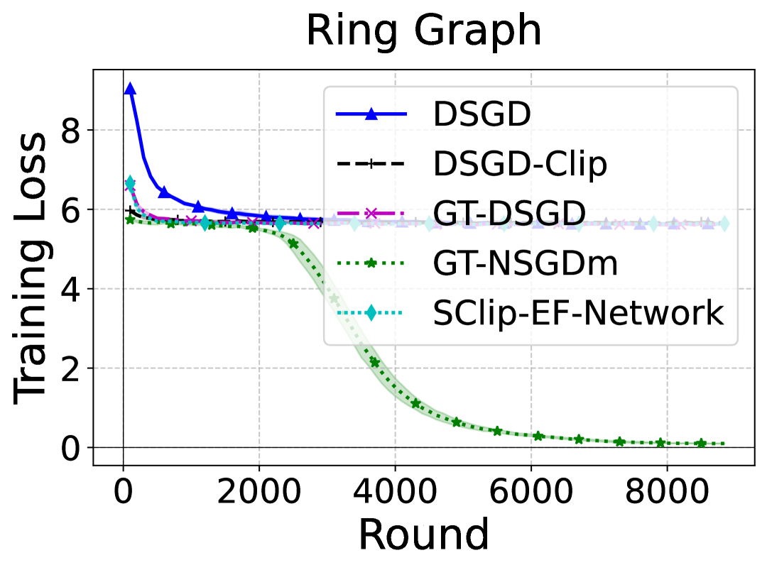
(a) Ring Graph

(b) Directed Exponential Graph

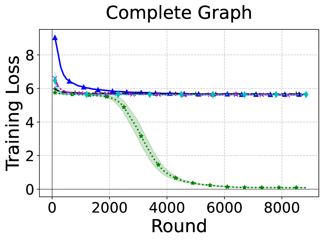
(c) Complete Graph

Figure 5: Comparison of graph-wide average training losses in decentralized training of Transformer models, over ring, directed exponential, and complete graphs.

Hyperparameter tuning. See Table 3 for our grid search range for algorithm hyperparameters.

Table 3: Hyperparameter grid search in decentralized training of Transformers

Method	Hyperparameter search set
DSGD	$\alpha\in\{10^{-4},5*10^{-4},10^{-3},5*10^{-3},10^{-2},5*10^{-2},10^{-1},0.5,1\}$
DSGD-Clip	$\alpha\in\{10^{-4},10^{-3},10^{-2},10^{-1},1,10,10^{2}\},\tau\in\{10^{-3},10^{-2},10^{-1},1,10,10^{2}\}$
GT-DSGD	$\alpha\in\{10^{-4},5*10^{-4},10^{-3},5*10^{-3},10^{-2},5*10^{-2},10^{-1},0.5,1\}$
GT-NSGDm	$\alpha\in\{10^{-4},10^{-3},10^{-2},10^{-1},1,10\},\beta\in\{0.01,0.2,0.4,0.6,0.8,0.99\}$
SClip-EF-Network	$\alpha\in\{10^{-4},10^{-3},10^{-2},10^{-1},10^{0},10^{1},10^{2}\},\beta\in\{0.01,0.4,0.8,0.99\},c_{\varphi}\in\{0.1,1,10,10^{2}\},\tau\in\{0.01,0.1,1,10\}$

Hardware. We simulate the distributed training on one NVIDA H100 GPU, using PyTorch 3.2 with CUDA 12. The total hyperparameter search and training procedure took around 100 GPU hours.

References

- [1] J. Tsitsiklis, D. Bertsekas, and M. Athans, “Distributed asynchronous deterministic and stochastic gradient optimization algorithms,” IEEE transactions on automatic control, vol. 31, no. 9, pp. 803–812, 1986.
- [2] A. Nedić, A. Olshevsky, and M. G. Rabbat, “Network topology and communication-computation tradeoffs in decentralized optimization,” Proceedings of the IEEE, vol. 106, no. 5, pp. 953–976, 2018.
- [3] T. Li, A. K. Sahu, A. Talwalkar, and V. Smith, “Federated learning: Challenges, methods, and future directions,” IEEE signal processing magazine, vol. 37, no. 3, pp. 50–60, 2020.
- [4] P. Kairouz, H. B. McMahan, B. Avent, A. Bellet, M. Bennis, A. N. Bhagoji, K. Bonawitz, Z. Charles, G. Cormode, R. Cummings, et al., “Advances and open problems in federated learning,” Foundations and Trends® in Machine Learning, vol. 14, no. 1–2, pp. 1–210, 2021.
- [5] T. S. Brisimi, R. Chen, T. Mela, A. Olshevsky, I. C. Paschalidis, and W. Shi, “Federated learning of predictive models from federated electronic health records,” International journal of medical informatics, vol. 112, pp. 59–67, 2018.
- [6] X. Lian, C. Zhang, H. Zhang, C.-J. Hsieh, W. Zhang, and J. Liu, “Can decentralized algorithms outperform centralized algorithms? a case study for decentralized parallel stochastic gradient descent,” Advances in neural information processing systems, vol. 30, 2017.
- [7] R. Xin, S. Pu, A. Nedić, and U. A. Khan, “A general framework for decentralized optimization with first-order methods,” Proceedings of the IEEE, vol. 108, no. 11, pp. 1869–1889, 2020.
- [8] S. Sundhar Ram, A. Nedić, and V. V. Veeravalli, “Distributed stochastic subgradient projection algorithms for convex optimization,” Journal of optimization theory and applications, vol. 147, pp. 516–545, 2010.
- [9] A. Koloskova, N. Loizou, S. Boreiri, M. Jaggi, and S. Stich, “A unified theory of decentralized sgd with changing topology and local updates,” in International Conference on Machine Learning, pp. 5381–5393, PMLR, 2020.
- [10] J. Wang and G. Joshi, “Cooperative sgd: A unified framework for the design and analysis of local-update sgd algorithms,” Journal of Machine Learning Research, vol. 22, no. 213, pp. 1–50, 2021.
- [11] K. Yuan, B. Ying, J. Liu, and A. H. Sayed, “Variance-reduced stochastic learning by networked agents under random reshuffling,” IEEE Transactions on Signal Processing, vol. 67, no. 2, pp. 351–366, 2018.
- [12] P. Di Lorenzo and G. Scutari, “Next: In-network nonconvex optimization,” IEEE Transactions on Signal and Information Processing over Networks, vol. 2, no. 2, pp. 120–136, 2016.
- [13] S. Pu and A. Nedić, “Distributed stochastic gradient tracking methods,” Mathematical Programming, vol. 187, no. 1, pp. 409–457, 2021.
- [14] A. Vaswani, N. Shazeer, N. Parmar, J. Uszkoreit, L. Jones, A. N. Gomez, Ł. Kaiser, and I. Polosukhin, “Attention is all you need,” Advances in neural information processing systems, vol. 30, 2017.
- [15] J. Nair, A. Wierman, and B. Zwart, The fundamentals of heavy tails: Properties, emergence, and estimation, vol. 53. Cambridge University Press, 2022.
- [16] U. Simsekli, L. Sagun, and M. Gurbuzbalaban, “A tail-index analysis of stochastic gradient noise in deep neural networks,” in International Conference on Machine Learning, pp. 5827–5837, PMLR, 2019.
- [17] J. Zhang, S. P. Karimireddy, A. Veit, S. Kim, S. Reddi, S. Kumar, and S. Sra, “Why are adaptive methods good for attention models?,” Advances in Neural Information Processing Systems, vol. 33, pp. 15383–15393, 2020.
- [18] E. Gorbunov, M. Danilova, and A. Gasnikov, “Stochastic optimization with heavy-tailed noise via accelerated gradient clipping,” Advances in Neural Information Processing Systems, vol. 33, pp. 15042–15053, 2020.
- [19] M. Gurbuzbalaban, U. Simsekli, and L. Zhu, “The heavy-tail phenomenon in sgd,” in International Conference on Machine Learning, pp. 3964–3975, PMLR, 2021.
- [20] K. Ahn, X. Cheng, M. Song, C. Yun, A. Jadbabaie, and S. Sra, “Linear attention is (maybe) all you need (to understand transformer optimization),” in The Twelfth International Conference on Learning Representations, 2024.
- [21] F. Kunstner, A. Milligan, R. Yadav, M. Schmidt, and A. Bietti, “Heavy-tailed class imbalance and why adam outperforms gradient descent on language models,” Advances in Neural Information Processing Systems, vol. 37, pp. 30106–30148, 2024.
- [22] Z. Charles, Z. Garrett, Z. Huo, S. Shmulyian, and V. Smith, “On large-cohort training for federated learning,” Advances in neural information processing systems, vol. 34, pp. 20461–20475, 2021.
- [23] H. Yang, P. Qiu, and J. Liu, “Taming fat-tailed (“heavier-tailed” with potentially infinite variance) noise in federated learning,” Advances in Neural Information Processing Systems, vol. 35, pp. 17017–17029, 2022.
- [24] A. Sadiev, M. Danilova, E. Gorbunov, S. Horváth, G. Gidel, P. Dvurechensky, A. Gasnikov, and P. Richtárik, “High-probability bounds for stochastic optimization and variational inequalities: the case of unbounded variance,” in International Conference on Machine Learning, pp. 29563–29648, PMLR, 2023.
- [25] E. M. Compagnoni, T. Liu, R. Islamov, F. N. Proske, A. Orvieto, and A. Lucchi, “Adaptive methods through the lens of SDEs: Theoretical insights on the role of noise,” in The Thirteenth International Conference on Learning Representations, 2025.
- [26] F. Hübler, I. Fatkhullin, and N. He, “From gradient clipping to normalization for heavy tailed sgd,” arXiv preprint arXiv:2410.13849, 2024.
- [27] Z. Liu and Z. Zhou, “Nonconvex stochastic optimization under heavy-tailed noises: Optimal convergence without gradient clipping,” in The Thirteenth International Conference on Learning Representations, 2025.
- [28] A. Armacki, S. Yu, P. Sharma, G. Joshi, D. Bajovic, D. Jakovetic, and S. Kar, “High-probability convergence bounds for online nonlinear stochastic gradient descent under heavy-tailed noise,” in The 28th International Conference on Artificial Intelligence and Statistics, 2025.
- [29] C. Sun and B. Chen, “Distributed stochastic strongly convex optimization under heavy-tailed noises,” in 2024 IEEE International Conference on Cybernetics and Intelligent Systems (CIS) and IEEE International Conference on Robotics, Automation and Mechatronics (RAM), pp. 150–155, IEEE, 2024.
- [30] S. Yu, D. Jakovetic, and S. Kar, “Smoothed gradient clipping and error feedback for decentralized optimization under symmetric heavy-tailed noise,” arXiv preprint arXiv:2310.16920, 2023.
- [31] D. Elliott, S. Frank, K. Sima’an, and L. Specia, “Multi30k: Multilingual english-german image descriptions,” arXiv preprint arXiv:1605.00459, 2016.
- [32] M. Barsbey, M. Sefidgaran, M. A. Erdogdu, G. Richard, and U. Simsekli, “Heavy tails in sgd and compressibility of overparametrized neural networks,” Advances in neural information processing systems, vol. 34, pp. 29364–29378, 2021.
- [33] B. Battash, L. Wolf, and O. Lindenbaum, “Revisiting the noise model of stochastic gradient descent,” in International Conference on Artificial Intelligence and Statistics, pp. 4780–4788, PMLR, 2024.
- [34] S. Peluchetti, S. Favaro, and S. Fortini, “Stable behaviour of infinitely wide deep neural networks,” in International Conference on Artificial Intelligence and Statistics, pp. 1137–1146, PMLR, 2020.
- [35] S. H. Lee, M. Zaheer, and T. Li, “Efficient distributed optimization under heavy-tailed noise,” arXiv preprint arXiv:2502.04164, 2025.
- [36] Z. Liu, J. Zhang, and Z. Zhou, “Breaking the lower bound with (little) structure: Acceleration in non-convex stochastic optimization with heavy-tailed noise,” in The Thirty Sixth Annual Conference on Learning Theory, pp. 2266–2290, PMLR, 2023.
- [37] T. D. Nguyen, T. H. Nguyen, A. Ene, and H. Nguyen, “Improved convergence in high probability of clipped gradient methods with heavy tailed noise,” Advances in Neural Information Processing Systems, vol. 36, pp. 24191–24222, 2023.
- [38] S. Chezhegov, Y. Klyukin, A. Semenov, A. Beznosikov, A. Gasnikov, S. Horváth, M. Takáč, and E. Gorbunov, “Gradient clipping improves adagrad when the noise is heavy-tailed,” arXiv preprint arXiv:2406.04443, 2024.
- [39] J. Duchi, E. Hazan, and Y. Singer, “Adaptive subgradient methods for online learning and stochastic optimization.,” Journal of machine learning research, vol. 12, no. 7, 2011.
- [40] D. P. Kingma and J. Ba, “Adam: A method for stochastic optimization,” arXiv preprint arXiv:1412.6980, 2014.
- [41] T. Sun, X. Liu, and K. Yuan, “Gradient normalization provably benefits nonconvex sgd under heavy-tailed noise,” arXiv preprint arXiv:2410.16561, 2024.
- [42] D. Jakovetić, D. Bajović, A. K. Sahu, S. Kar, N. Milosević, and D. Stamenković, “Nonlinear gradient mappings and stochastic optimization: A general framework with applications to heavy-tail noise,” SIAM Journal on Optimization, vol. 33, no. 2, pp. 394–423, 2023.
- [43] A. Armacki, S. Yu, D. Bajovic, D. Jakovetic, and S. Kar, “Large deviations and improved mean-squared error rates of nonlinear sgd: Heavy-tailed noise and power of symmetry,” arXiv preprint arXiv:2410.15637, 2024.
- [44] E. Gorbunov, A. Sadiev, M. Danilova, S. Horváth, G. Gidel, P. Dvurechensky, A. Gasnikov, and P. Richtárik, “High-probability convergence for composite and distributed stochastic minimization and variational inequalities with heavy-tailed noise,” 2024.
- [45] E. M. Compagnoni, R. Islamov, F. N. Proske, and A. Lucchi, “Unbiased and sign compression in distributed learning: Comparing noise resilience via SDEs,” in The 28th International Conference on Artificial Intelligence and Statistics, 2025.
- [46] S. Yu and S. Kar, “Secure distributed optimization under gradient attacks,” IEEE Transactions on Signal Processing, 2023.
- [47] B. Li and Y. Chi, “Convergence and privacy of decentralized nonconvex optimization with gradient clipping and communication compression,” IEEE Journal of Selected Topics in Signal Processing, 2025.
- [48] T. Yang, X. Yi, J. Wu, Y. Yuan, D. Wu, Z. Meng, Y. Hong, H. Wang, Z. Lin, and K. H. Johansson, “A survey of distributed optimization,” Annual Reviews in Control, vol. 47, pp. 278–305, 2019.
- [49] L. Bottou, F. E. Curtis, and J. Nocedal, “Optimization methods for large-scale machine learning,” SIAM review, vol. 60, no. 2, pp. 223–311, 2018.
- [50] A. Radford, K. Narasimhan, T. Salimans, I. Sutskever, et al., “Improving language understanding by generative pre-training,” 2018.
- [51] R. Xin, U. A. Khan, and S. Kar, “Variance-reduced decentralized stochastic optimization with accelerated convergence,” IEEE Transactions on Signal Processing, vol. 68, pp. 6255–6271, 2020.
- [52] A. Olshevsky, “Linear time average consensus on fixed graphs and implications for decentralized optimization and multi-agent control,” arXiv preprint arXiv:1411.4186, 2014.
- [53] B. Gharesifard and J. Cortés, “Distributed strategies for generating weight-balanced and doubly stochastic digraphs,” European Journal of Control, vol. 18, no. 6, pp. 539–557, 2012.
- [54] M. Assran, N. Loizou, N. Ballas, and M. Rabbat, “Stochastic gradient push for distributed deep learning,” in International Conference on Machine Learning, pp. 344–353, PMLR, 2019.
- [55] A. Nedic and A. Ozdaglar, “Distributed subgradient methods for multi-agent optimization,” IEEE Transactions on Automatic Control, vol. 54, no. 1, pp. 48–61, 2009.
- [56] C. Sun, “Distributed stochastic optimization under heavy-tailed noises,” arXiv preprint arXiv:2312.15847, 2023.
- [57] L. Xiao, S. Boyd, and S. Lall, “A scheme for robust distributed sensor fusion based on average consensus,” in IPSN 2005. Fourth International Symposium on Information Processing in Sensor Networks, 2005., pp. 63–70, IEEE, 2005.
- [58] A. E. Beaton and J. W. Tukey, “The fitting of power series, meaning polynomials, illustrated on band-spectroscopic data,” Technometrics, vol. 16, no. 2, pp. 147–185, 1974.