Critical habitat size of organisms diffusing with stochastic resetting
Abstract
The persistence of populations depends on the minimum habitat area required for survival, known as the critical patch size. While most studies assume purely diffusive movement, additional movement components can significantly alter habitat requirements. Here, we investigate how critical patch sizes are affected by stochastic resetting, where each organism intermittently returns to a common fixed location, modeling behaviors such as homing, refuge-seeking, or movement toward essential resources. We analytically derive the total population growth over time and the critical patch size. Our results are validated by agent-based simulations, showing excellent agreement. Our findings demonstrate that stochastic resetting can either increase or decrease the critical patch size, depending on the reset rate, reset position, and external environmental hostility. These results highlight how intermittent relocation shapes ecological thresholds and may provide insights for ecological modeling and conservation planning, particularly in fragmented landscapes such as in deforested regions.
I Introduction
The critical patch size problem involves determining the minimum area required for a population of moving organisms to survive in a habitat surrounded by a hostile or unfavorable environment [1, 2, 3, 4]. As such, it is a fundamental concept in spatial population dynamics, crucial to understanding species persistence in fragmented landscapes [5] and to developing strategies to mitigate its impacts [6, 7, 8]. The critical size arises from the competition between population growth in the viable region and dispersal in the hostile environment [9]. In its simplest form, the mathematical formulation of the problem amounts to considering population growth and diffusive spread across a boundary into an absorbing region [10]. Its solution corresponds to finding the maximal eigenvalue of the Laplacian operator with Dirichlet boundary conditions. From this perspective, this question is crucial not only in population dynamics but also in both theoretical and applied contexts across a wide range of disciplines.
The critical size problem has been examined under various conditions, including inhomogeneous environments [11, 12, 13], environmental conditions stochasticity [14, 15], periodic oscillations [16, 17], and the presence of movement bias [18], among others [19]. These studies provide valuable information on how different environmental factors influence population persistence. In fact, in real-world ecosystems, individuals often experience disruptions, such as environmental fluctuations or other forms of stochasticity, which can significantly impact their survival prospects. An important form of sudden disruption is the sporadic return of an organism to a preferred location or state in the system. One example are scenarios with predator-prey encounters [20], which can be modeled by stochastic resetting [21, 22] of the individual’s position. This reset can also be associated with occasional recolonization or migration and with behaviors such as central-place foraging [23]. The reset location can also represent resources such as a watering hole or a salt-lick.
Understanding how such resetting processes influence critical habitat sizes can provide insights into population persistence under uncertain conditions. In particular, stochastic resetting of position can allow an individual to overcome temporary resource scarcity or adverse conditions, potentially reducing the amount of space required for population survival. The existence of such a preferred location to which individuals return aligns well with field observations which show that individuals often have a tendency to concentrate around certain habitat regions [24]. In this study, we investigate the impact of stochastic resetting of position, taking as control parameters both the rate and position to which the individuals reset, on the critical habitat size of populations diffusing in one dimension.
By examining the interplay between resetting dynamics and habitat properties, we aim to gain understanding about ecological resilience and population sustainability in more realistic scenarios. At the same time, by incorporating the stochastic reset mechanism, we aim to contribute to a broader framework in which the Laplacian problem is applicable, extending its relevance to more complex, real-world scenarios.
The model is defined in Section II. In Section III, we examine the scenario under extreme external conditions, where the population decays at an infinite extinction rate , which can be effectively modeled by setting absorbing boundary conditions. We also consider the general case with arbitrary , presented in Section IV. In both scenarios, we explore how varying the reset rate and reset position influences the habitat size at which the population transitions to extinction, providing insight into the role of reset dynamics in population viability. Final remarks and conclusions are presented in Section V.
II Model
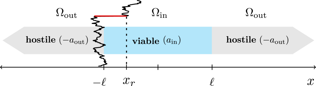
In one dimension, we define a good-quality region—referred to as patch or habitat—as the interval . In the habitat, the population grows at a rate . This region is surrounded by a hostile environment (the complement set of , denoted by ), where the growth rate is negative, , as depicted in Fig. 1. Organisms move via normal diffusion plus sporadic random relocation from a pre-defined region to a fixed position either inside or outside the habitat. For the region from where reset occurs, two cases will be considered. The first will be the entire space and the second just the outside region . Moreover, we assume that the resets take place at random intervals, following a Poisson process with rate , and each reset brings the walker to the fixed location .
Using a discrete, agent-based description, we have that the movement of an organism follows a Brownian motion supplemented with stochastic resetting, which can be mathematically described as follows:
| (3) |
where is the diffusivity, assumed to be the same everywhere, and is a Gaussian noise with zero mean and unit variance. For population growth, we employ the reactions
| if | |||||
| (4) |
where is a new individual and denotes death. Furthermore, we consider that at all walkers start at a position .
Alternatively, the dynamics can be described in the continuum limit in terms of the density of organisms per unit length, , which represents the number of individuals per unit length at position and time , given an initial position . Following the lines of Ref. [21, 25], is governed by the reaction-diffusion equation given by
| if | |||||
| (5) |
where , and (or 0) if contains (or not). In addition, we rescaled the variables and parameters as follows: , , (), and . Note that in Eq. (5), the term with the Dirac delta vanishes in one of the equations since belongs to one of the two regions only.
In the equation for , the first term represents diffusion, the second term accounts for the growth at unit rate within the viable region together with the reduction due to organisms being relocated, while the last term gives the contribution from resets at position , which is nonzero only if . In the equation for , the first term again represents diffusion, the second reflects the decay due to the negative rate along with the removal of organisms via resetting, and the third term is the contribution from resets at , which is nonzero only if .
Notice that we define the problem as linear from the outset, disregarding carrying capacity terms; however, our approach can be extended to more general scenarios (such as those involving logistic growth). Since we are primarily concerned with the critical condition near which the population density is very low, the carrying capacity will have no effect.
III Totally hostile environment
We first assume that, outside the good-quality patch, i.e., for , one has that , which means that organisms that leave the patch are instantly killed. Thus, only the first of the two equations in Eq. (5) matters, i.e., the one for , with . The external region is mimicked by absorbing boundary conditions at . Let us write the backward master equation associated to this process [26, 25]:
| (6) |
where we denote . Then, integrating over , we obtain the following differential equation for the total number of organisms ,
| (7) |
The detailed steps for solving these equations are provided in the Appendixes. For sufficiently large times, we obtain
| (8) |
where is a constant that depends on all the parameters of the model, and is the dominant growth rate of a spectrum, which depends on , and (see Appendix A for details on the calculations).
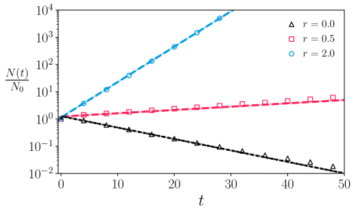
In Fig. 2, we plot the evolution of for different values of the reset rate . Symbols correspond to numerical simulations of the stochastic process defined by Eqs. (3), while the dashed lines are given by the theoretical prediction provided by Eq. (8), in good agreement with the simulations. In the case of Fig. 2 ( and , which, in the absence of resetting, is slightly subcritical), we observe that the population decays, and the same happens for low reset rates. Conversely, for reset rates above a critical threshold (), the population exhibits growth.
III.1 Critical size
At the critical condition that separates the regimes of persistence and decline of the population, a stationary state corresponding to emerges. The critical size can be directly obtained by solving the stationary form of Eq. (7) (see Appendix B), leading to
| (9) |
where (and throughout the rest of the paper) the functions are defined for complex argument. The special (resonant) case , for which the reset rate equals the growth rate, can be obtained by taking the limit , which yields . Setting , we recover the well-known result in the absence of resetting: .
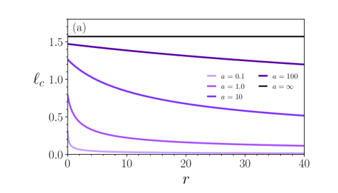
Regarding the effect of the rate on the critical size for fixed reset position , we present in Fig. 3(a) a plot of vs. for different values of . Essentially, three different behaviors can be observed.
In particular, when , Eq. (9) becomes
| (10) |
which decays with as shown in Fig. 3(a). In the limit , one has . The same occurs for other reset positions provided that the slope , i.e., for . This range defines a core region around the center () where any resetting favors survival in a smaller habitat than in the reset-free case.
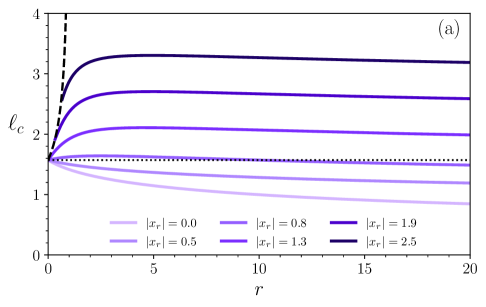
For sufficiently far from the center, stochastic reset cannot reduce the critical size regardless of the value of . In fact, first increases with reaching a maximum and then decays to , which is equal to , according to Eq. (9). Therefore, for , habitat reduction cannot occur.
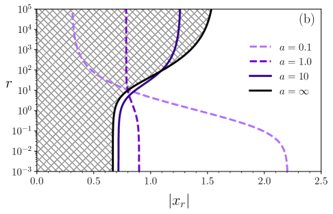
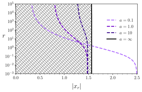
In the intermediate region , although first increases with , then, after reaching a maximum, it decays below the reset-free value . This occurs provided that the reset rate is sufficiently high, namely, above the threshold rate , at which . This corresponds to the point where each curve in Fig. 3(a) intersects the dashed horizontal line. The threshold is plotted vs. in Fig. 3(b) (solid black line for ). It indicates that, to prevent extinction, large rates are required when is located outside a core region around the habitat center. The double-hashed region is where the reset mechanism, characterized by and , allows a reduction in habitat size.
Let us remark that a nonmonotonic behavior, as observed in Fig. 3 for sufficiently far from the boundaries, resembles that seen in scenarios where an elastic force guides organisms towards a specific area known as home range [18]. In that case, increasing the stiffness plays a similar role to increasing the reset rate in our problem. For weak forces, this effect can increase or decrease the critical patch size. However, when the force amplitude is sufficiently strong, organisms tend to concentrate in the return position.
Finally, let us remark that, when the reset position is outside the patch, , then, according to Eq. (5), the effect of resetting is to effectively reduce the reproduction rate from . This still allows survival for at a larger critical size given by the reset-free expression with :
| (11) |
of course, independent of the reset position, since is in the absorbing region. This condition can occur only for . In fact, setting , the non-null solution is , plotted in Fig. 3(a) as a dashed curve.
In summary:
(i) For , the critical size is reduced by resetting at any rate (that is, ).
(ii) For , the critical size can be reduced for rates .
(iii) For , the critical size cannot be reduced for any .
III.2 Stationary spatial distribution at criticality
For a sufficiently long time, when the dominant mode has settled (which can occur very quickly, as observed in Fig. 2), we can approximate , which substituted into Eq. (5) gives
| (12) |
where was defined in Eq. (29). The solution of Eq. (12) is the Green function associated to the 1D Helmholtz equation, that is,
| (13) |
where (see Appendix A). The initial assumption implies that the spatial profile tends to a shape that remains unchanged except for the exponential pre-factor.
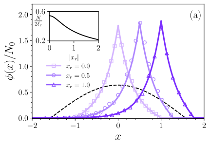
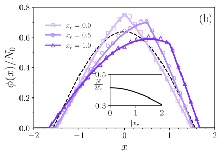
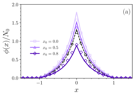
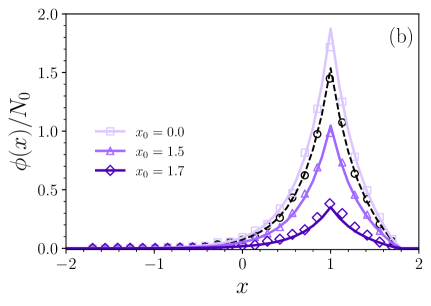
At criticality, where and , coincides with the stationary solution. These theoretical stationary profiles are shown in Fig. 4 (lines), for (a) and (b), and different values of , in good agreement with the agent-based simulations. Note again that, for reset positions near the center (small ), the reset mechanism reduces the critical habitat size. However, this effect is not observed for positions closer to the borders. Furthermore, the stationary value of the total population density, , decreases with increasing , as illustrated in the insets.
III.3 Role of the initial distribution
Recall that the initial condition considered is a Dirac delta function at an arbitrary point in the high quality region, but Eq. (9) for the critical patch size remains independent of this initial concentration point.
Fig. 5(a) shows the steady states resulting from initial conditions concentrated at different initial points , for the reset position and . Note that the shape is invariant but its height decreases when the reset position is shifted towards the borders, as expected due to larger diffusive losses during the transient. The case of uniform initial distribution is also plotted for comparison, yielding also the same stationary profile except for a multiplicative factor. Also in this case the critical habitat size is unchanged. In fact, since any general initial distribution can be represented as a continuous superposition of Dirac delta functions, and the evolution equation is linearized, then, in particular, the critical size is unaffected by the choice of initial distribution, as illustrated by the stationary spatial profile that emerges from the uniform distribution. Fig. 5(b) illustrates the effect of the initial condition for an off-center resetting position (), displaying qualitatively similar effects to those in case (a).
IV Partially hostile environment
We now consider scenarios in which the region outside the patch of size is not completely degraded, but instead has finite extinction rate , while stochastic returns can occur from a given region to a position within or outside the patch. We analyze two main relevant cases, for which we find the critical habitat size. One of them is when , that is, organisms both inside and outside the habitat can be reset, what we call “total relocation”. Another is when , that is, only the organisms in the external region can be reset, what we name “partial relocation”.
IV.1 Total relocation
Organisms inside and outside the patch can be selected for sudden relocation. Then, Eqs. (5) become
| (14) |
If , that is, if organisms are relocated to the patch, we obtain (following the approach described in Appendix C),
| (15) |
where
with and .
If , that is, if organisms are relocated to a point outside the patch, then a transcendental equation for the critical size is obtained, namely,
| (16) |
where .
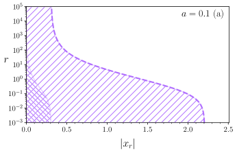
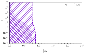
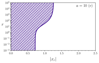
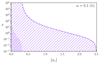
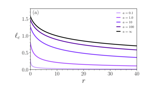
Figure 6(a) shows the critical half-width as a function of , for the special case and different values of . In the absence of resetting, less hostile environments (i.e., lower decay rate ) lead, of course, to a reduced critical size. When reset is introduced and , then the increase in the reset rate monotonically reduces , as expected since more frequently organisms are conducted to the most favorable point. This effect is more pronounced for smaller values of . In particular, when approaches zero, the critical size tends to zero as well. In the opposite limit , we recover the curve for shown in Fig. 3(a).
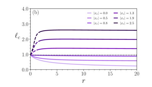

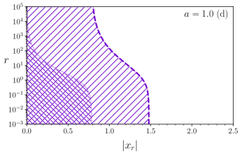
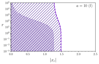
For other values of , the curves vs. can exhibit several different nonmonotonic behaviors, as shown in Figs. 6(b)-(c). For (b), the picture is qualitatively similar to that observed for the totally hostile environment in Fig. 3, with the three types of regime described at the end of Sect. III.1. We remark that the dashed line for was obtained by numerically solving Eq. (16), which recapitulates Eq. (11) when . In this limit, the full portrait provided by Fig. 3(a) is recovered.
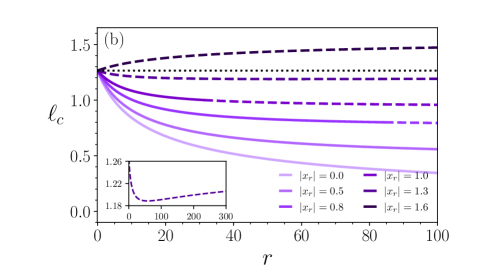
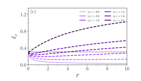
However, when the environment is weakly hostile (i.e., is small), the picture departs from that of the totally hostile environment, as illustrated in Fig. 6(c), for . Typically, for small enough , there is an optimal (finite) reset rate, which produces a minimal critical size (hence smaller than the reset-free one) for resetting positions outside the habitat (dashed lines), as illustrated for in Fig. 6(c). This effect can be qualitatively understood as follows. For a highly hostile environment (large ), resetting becomes detrimental when the reset position is located far from the patch center, even if it is still within the patch. In such cases, survival requires an increase in habitat size. Differently, in a weakly hostile environment (small ), there can be a positive balance of individuals that benefit from being reset to a position close to the patch, even if outside the patch, so that they do not spend too much time well within the outside region. In such case, the reset dynamics can lead to a reduction in the minimal habitat size. This balance involves the timescales of the reset, growth and diffusive processes. However, if the reset position is too distant or the reset rate becomes too high, this balance is reversed, and a minimum habitat size emerges at that tipping point.
The results are summarized in the diagram of Fig. 3(b), where we present, for each value of , the line that delimits the region in the plane of parameters –, for which resetting reduces , depicted by a dashed line when or by a solid line when . Moreover, for , we distinguish the regions where the reduction occurs, depending on whether lies inside (double-hashed) or outside (hashed) the patch. The line that delimits the two regions is obtained by setting in Eq. (15), or alternatively in Eq. (16), yielding
IV.2 Partial relocation
In this case, only organisms localized in the external region are repositioned. In such a case , and the stationary form of Eqs. (5) become
| (18) |
Following the same approach as in Sec IV.1, if , that is, if organisms are relocated to the patch, then the critical size is given by
| (19) |
where .
If relocations are from outside the patch, i.e., , then the critical half-width is obtained by numerically solving the equation
| (20) |
where .
Figure 7(a) shows the critical half-width as a function of , for and different values of . The picture is qualitatively similar to that observed in Fig. 6(a). However, in this case the reset mechanism is less effective in reducing the critical size, as can be seen by the slower decay and lower ratio for the same value of . In the limit , becomes independent of , in contrast to the case of total relocation. Note that only individuals in the hostile region are “rescued” in the present case.
When changing , new nonmonotonic behaviors of vs. emerge, as shown in Fig. 6(b). Even when the reset position is outside the patch (dashed lines), resetting can be beneficial. Furthermore, for certain values of (outside the patch), there is an optimal rate for which is minimal (as illustrated in the inset for ), smaller than in the reset-free case. The appearance of this optimal value can be understood by similar arguments to those used in relation to the optimal values in Fig. 6. The full portrait is schematized in Fig. 8, where we plot, for each value of in the legend, the curve that defines the region where reset reduces the critical size (to the left of the curve).
The line that delimits the two regions is obtained by setting in Eq. (19), or alternatively in Eq. (20), yielding
| (21) |
V Conclusions and final remarks
We studied the effects of stochastic resetting in the critical patch size problem. Organisms can be subject to stochastic spatial repositioning into or to the outside of a viable patch. We first focused on the specific scenario of an extremely hostile environment beyond the boundaries of a good-quality region. We obtained a robust analytical approximation to describe the dynamics of the total population over time, providing insight into the long-term behavior of the population in such extreme environments. Furthermore, we analytically derived an explicit expression for the critical patch size, , as a function of the parameters of the population dynamics and stochastic resetting.
Next, we extended our study to address a more general scenario, where the environment outside the habitat is not entirely lethal but is characterized by a finite mortality rate. This scenario is particularly relevant for real-world ecosystems, where habitats often exist in a complex mosaic of varying environmental conditions. We elaborated the cases where organisms can be relocated from the outside or from anywhere, into the patch or outside it. In some cases, we arrive at a closed form expression for the critical habitat size, while in other ones we obtained a transcendental equation from which can be numerically extracted.
In some cases, we observe that the critical size can decrease with resetting, the more the higher are the reset rates. In other cases, depending on , there may also be a pessimal scenario in which there is a reset rate that makes the critical size reach its maximum value. These regimes were clearly delineated using our analytical results. Similar results are obtained for the partially hostile environment, when is large. However, for small , a minimal emerges at a finite optimal rate when organisms relocate to the outer region.
These results deepen our understanding of how environmental structure and stochastic sporadic events jointly influence population persistence in fragmented or degraded landscapes. One key consequence of our findings is the identification of non-monotonic dependencies between resetting rate and critical habitat size, revealing that movement strategies based on intermittent relocation can either facilitate survival or exacerbate extinction risks, depending on both the reset location and the environmental hostility. This challenges the classical intuition that more frequent returns to a safe location always enhance survival, highlighting instead the subtle interplay between movement dynamics and spatial context. As future perspectives, a whole research line becomes possible, such as considering scenarios with heterogeneous environments[12, 29], density-dependent processes [11, 30], non-instantaneous resetting [31, 32, 33] or considering a distribution of reset positions.
Acknowledgments
We all acknowledge partial financial support by the Coordenação de Aperfeiçoamento de Pessoal de Nível Superior - Brazil (CAPES) - Finance Code 001. C.A. also acknowledges the partial financial support (311435/ 2020-3) of Conselho Nacional de Desenvolvimento Científico e Tecnológico (CNPq), Brazil, and (CNE E-26/204.130/2024) Fundação de Amparo à Pesquisa do Estado do Rio de Janeiro (FAPERJ), Brazil. P.d.C. was supported by Scholarships No. 2021/10139-2 and No. 2022/13872-5 and ICTP-SAIFR Grant No. 2021/14335-0, all granted by São Paulo Research Foundation (FAPESP), Brazil.
References
- MacArthur and Wilson [2001] R. H. MacArthur and E. O. Wilson, The theory of island biogeography, Vol. 1 (Princeton university press, 2001).
- Tilman [1994] D. Tilman, Competition and biodiversity in spatially structured habitats, Ecology 75, 2 (1994).
- Hanski [1999] I. Hanski, Metapopulation ecology (Oxford University Press, 1999).
- Fahrig [2003] L. Fahrig, Effects of habitat fragmentation on biodiversity, Annual review of ecology, evolution, and systematics 34, 487 (2003).
- Franklin et al. [2002] A. B. Franklin, B. R. Noon, and T. L. George, What is habitat fragmentation?, Studies in avian biology 25, 20 (2002).
- Pimm and Jenkins [2019] S. L. Pimm and C. N. Jenkins, Connecting habitats to prevent species extinctions, American Scientist 107, 162 (2019).
- Ibagon et al. [2022] I. Ibagon, A. Furlan, and R. Dickman, Reducing species extinction by connecting fragmented habitats: Insights from the contact process, Physica A: Statistical Mechanics and its Applications 603, 127614 (2022).
- Cantrell and Cosner [1999] R. Cantrell and C. Cosner, Diffusion models for population dynamics incorporating individual behavior at boundaries: applications to refuge design, Theoretical population biology 55, 189 (1999).
- Cantrell and Cosner [2001] R. Cantrell and C. Cosner, Spatial heterogeneity and critical patch size: area effects via diffusion in closed environments, Journal of Theoretical Biology 209, 161 (2001).
- Kierstead and Slobodkin [1953] H. Kierstead and L. Slobodkin, The size of water masses containing plankton blooms, Journal of Marine Research (1953).
- Colombo and Anteneodo [2018] E. Colombo and C. Anteneodo, Nonlinear population dynamics in a bounded habitat, Journal of Theoretical Biology 446, 11 (2018).
- dos Santos et al. [2020] M. A. F. dos Santos, V. Dornelas, E. H. Colombo, and C. Anteneodo, Critical patch size reduction by heterogeneous diffusion, Phys. Rev. E 102, 042139 (2020).
- Lin et al. [2004] A. L. Lin, B. A. Mann, G. Torres-Oviedo, B. Lincoln, J. Käs, and H. L. Swinney, Localization and extinction of bacterial populations under inhomogeneous growth conditions, Biophysical Journal 87, 75 (2004).
- Méndez et al. [2010] V. Méndez, I. Llopis, D. Campos, and W. Horsthemke, Extinction conditions for isolated populations affected by environmental stochasticity, Theoretical Population Biology 77, 250 (2010).
- Berti et al. [2015] S. Berti, M. Cencini, D. Vergni, and A. Vulpiani, Extinction dynamics of a discrete population in an oasis, Phys. Rev. E 92, 012722 (2015).
- Ballard et al. [2004] M. Ballard, V. M. Kenkre, and M. N. Kuperman, Periodically varying externally imposed environmental effects on population dynamics, Phys. Rev. E 70, 031912 (2004).
- Colombo and Anteneodo [2016] E. H. Colombo and C. Anteneodo, Population dynamics in an intermittent refuge, Phys. Rev. E 94, 042413 (2016).
- Dornelas et al. [2024] V. Dornelas, P. de Castro, J. M. Calabrese, W. F. Fagan, and R. Martinez-Garcia, Movement bias in asymmetric landscapes and its impact on population distribution and critical habitat size, Proceedings of the Royal Society A 480, 10.1098/rspa.2024.0185 (2024).
- Neicu et al. [2000] T. Neicu, A. Pradhan, D. A. Larochelle, and A. Kudrolli, Extinction transition in bacterial colonies under forced convection, Phys. Rev. E 62, 1059 (2000).
- Mercado-Vásquez and Boyer [2018] G. Mercado-Vásquez and D. Boyer, Lotka–volterra systems with stochastic resetting, Journal of Physics A: Mathematical and Theoretical 51, 405601 (2018).
- Evans and Majumdar [2011a] M. R. Evans and S. N. Majumdar, Diffusion with stochastic resetting, Phys. Rev. Lett. 106, 160601 (2011a).
- Evans et al. [2020] M. R. Evans, S. N. Majumdar, and G. Schehr, Stochastic resetting and applications, Journal of Physics A: Mathematical and Theoretical 53, 193001 (2020).
- Bell [1990] W. J. Bell, Central place foraging, in Searching Behaviour: The behavioural ecology of finding resources (Springer Netherlands, Dordrecht, 1990) pp. 171–187.
- Van Moorter et al. [2016] B. Van Moorter, C. M. Rolandsen, M. Basille, and J.-M. Gaillard, Movement is the glue connecting home ranges and habitat selection, Journal of Animal Ecology 85, 21 (2016).
- Evans and Majumdar [2011b] M. R. Evans and S. N. Majumdar, Diffusion with optimal resetting, Journal of Physics A: Mathematical and Theoretical 44, 435001 (2011b).
- Gardiner et al. [1985] C. W. Gardiner et al., Handbook of stochastic methods, Vol. 3 (springer Berlin, 1985).
- [27] Obtained numerically by de Hoog method [34].
- Skellam [1991] J. Skellam, Random dispersal in theoretical populations, Bulletin of Mathematical Biology 53, 135 (1991).
- Menon and Anteneodo [2024] L. Menon and C. Anteneodo, Random search with resetting in heterogeneous environments, Phys. Rev. E 110, 054111 (2024).
- Piva and Anteneodo [2025] G. Piva and C. Anteneodo, Influence of density-dependent diffusion on pattern formation in a refuge, Physica A: Statistical Mechanics and its Applications 658, 130305 (2025).
- Bodrova and Sokolov [2020] A. S. Bodrova and I. M. Sokolov, Resetting processes with noninstantaneous return, Physical Review E 101, 052130 (2020).
- Mercado-Vásquez et al. [2020] G. Mercado-Vásquez, D. Boyer, S. N. Majumdar, and G. Schehr, Intermittent resetting potentials, Journal of Statistical Mechanics: Theory and Experiment 2020, 113203 (2020).
- Gupta et al. [2021] D. Gupta, A. Pal, and A. Kundu, Resetting with stochastic return through linear confining potential, Journal of Statistical Mechanics: Theory and Experiment 2021, 043202 (2021).
- De Hoog et al. [1982] F. R. De Hoog, J. H. Knight, and A. Stokes, An improved method for numerical inversion of laplace transforms, SIAM Journal on scientific and Statistical Computing 3, 357 (1982).
- Butkov [1973] E. Butkov, Mathematical physics (Addison-Wesley Publ., Reading, Mass, 1973).
- Ludwig et al. [1979] D. Ludwig, D. Aronson, and H. Weinberger, Spatial patterning of the spruce budworm, Journal of Mathematical Biology 8, 217 (1979).
Appendix A Solving Eq. (7)
We proceed to solve Eq. (7) by Laplace transforming in time, which yields
| (22) |
where is the initial population. The general solution of Eq. (22) is
| (23) | |||||
where functions are defined for complex argument.
Since vanishes for the initial conditions , then, and
| (24) |
Furthermore, Eq. (23) must be solved self-consistently, by setting , which yields
| (25) |
with .
Finally, Laplace transform inversion can be obtained by the Mellin integral
| (26) |
where is a suitable real constant [35]. The integrand in Eq. (26) exhibits a singularity structure characterized by poles determined as the solutions of
| (27) |
which are real valued and can be obtained numerically. In the absence of reset (), Eq. (27) yields , with , and Eq. (26) recovers the known result [28, 36], namely .
For large , the dominant contribution to inversion will be determined by the largest pole . By applying Cauchy’s residue theorem for this pole, we obtain
| (28) |
where is given by
| (29) |
where and is the initial total population.
Appendix B Solving the stationary form of Eq. (7)
An alternative approach to deriving consists in solving the stationary form of Eq. (7), namely,
| (30) |
with the boundary conditions .
For , we obtain
| (31) |
By setting , for consistency, we directly obtain, in an alternative way, Eq. (9).
Appendix C Stationary solution for a partially hostile environment
In all cases, to address the stationary problem, we begin by setting Eqs. (5) equal to zero. Owing to their linear structure, the solutions in each region take the form of real exponential functions in the outer domains, and a combination of sine and cosine functions (either with real or imaginary arguments, depending on the parameters) within the patch.
The solutions must verify continuity at and at . Additionally, the flux must be continuous at , which imposes . At , the presence of a Dirac delta introduces a discontinuity in the derivative, leading to a jump condition . These six conditions lead to a homogeneous system of equations for the coefficients. To obtain nontrivial solutions, the determinant of the resulting coefficient matrix must vanish. This condition determines the value of .
The procedure is illustrated for the case of Eq. (18). When , the stationary solution is
| (34) |
with . The continuity and boundary conditions explicitly are
where
Using Eq. (34), these conditions can be written in matrix form as , where
| (35) |
Since the system is homogeneous, a nontrivial solution, requires , which leads to the equation
| (36) |
from which can be extracted, yielding Eq. (19).
For the case , the solution of Eq. (18) has the form
| (37) |
Applying the corresponding continuity and boundary conditions to produce the matrix (not shown), the condition of null determinant leads to the transcendental Eq. (20), which was solved numerically.
We proceed analogously in the cases where repositions can occur from any place. The main difference is that the argument for the and functions is (which for leads to hyperbolic functions), and that the jump in the derivative due to the Dirac delta is proportional to the total , instead of . Then, for , the matrix singularity condition leads to
| (38) |
which can be solved for to obtain the closed form Eq. (15), while for , the matrix singularity condition yields the transcendental Eq. (16).
Appendix D Phase diagrams