Stay Positive: Neural Refinement of Sample Weights

Abstract

Monte Carlo simulations are an essential tool for data analysis in particle physics. Simulated events are typically produced alongside weights that redistribute the cross section across the phase space. Latent degrees of freedom introduce a distribution of weights at a given point in the phase space, which can include negative values. Several post-hoc reweighting methods have been developed to eliminate the negative weights. All of these methods share the common strategy of approximating the average weight as a function of phase space. We introduce an alternative approach with a potentially simpler learning task. Instead of reweighting to the average, we refine the initial weights with a scaling transformation, utilizing a phase space-dependent factor. Since this new refinement method does not need to model the full weight distribution, it can be more accurate. High-dimensional and unbinned phase space is processed using neural networks for the refinement. Using both realistic and synthetic examples, we show that the new neural refinement method is able to match or exceed the accuracy of similar weight transformations.

I Introduction

Statistical analysis in particle physics usually involves the comparison of simulated and recorded data. The simulated data are generated with Monte Carlo methods, and the events are often weighted due to the complex nature of the underlying physics. The weights themselves are not physical and only the sum of all weights at a given phase-space point corresponds to an observable. The spread of weights reduces the statistical power of a synthetic dataset. Sometimes, weights can be negative. As cross sections are non-negative, the existence of negative weights implies a spread in weights and thus a dilution in statistical power. Negative weights may also lead to other complications in downstream analyses. There are multiple origins of negative weights, including higher-order perturbative corrections and background subtraction.

A number of methods have been proposed to reduce the contribution from negative weights. For example, multiple algorithm-specific modifications to higher-order calculations have been studied for reducing negative weight contributions [1, 2, 3]. A complementary approach are algorithm-agnostic techniques that reduce negative weights post-hoc [4, 5, 6, 7, 8]. These tools can also have desirable statistical properties like uncertainty conservation [5]. All of these methods have a similar strategy - the weight $w_{i}$ for event $i$ is replaced by the average weight for the corresponding point in phase space $x_{i}$. A key challenge with these approaches is that this reassignment of weights can be highly non-trivial, especially if the conditional probability density $p(w|x)$ has a large variance.

We make a simple, but powerful observation that instead of reweighting events by replacing $w_{i}$ with the average, we can refine the $w_{i}$ of each event to remove negative weights. An extreme example, which we will discuss in more detail below, is the case where there is a non-trivial $p(w|x)$, yet all weights are non-negative. Reweighting methods still act non-trivially on such events, while our new strategy can leave them unchanged. This weight refining has a number of practical advantages over reweighting that we will highlight with numerical examples. We use neural networks in all our examples since they scale well to many dimensions, but the refinement strategy can be adapted to any local estimation of weights. Our approach is also compatible with the resampling protocol of Ref. [5] for matching uncertainties; however, we omit its implementation here to facilitate a direct comparison of different methods.

This paper is organized as follows. Section II introduces the formal properties of reweighting and refinement. Numerical examples are provided in section III and the paper ends with conclusions and and outlook in section IV.

II Neural Refinement

First, we briefly review neural reweighting before introducing weight refinement. The goal of reweighting is to replace weights $w_{i}$ by $\int\text{d}x\,p(z|x)w(z,x)$, where the latent variable $z$ is the source of randomness for the weights at a fixed phase space point $x$. In other words, reweighting replaces individual weights by the average weight for a given phase space point $x=x_{i}$. This can be accomplished with the following loss functional:

$$\mathcal{L}[g]= -\int\text{d}x\text{d}z\,p(x,z)w(x,z)\log(g(x))$$

$$\hskip 5.69054pt-\int\text{d}x\,p(x)\log(1-g(x))\,,$$ (1)

where we are working in the continuum limit where a sum over events is replaced with an integral weighted by the probability density as this simplifies the functional analysis. Equation 1 is the standard binary cross entropy, but with the same events in both terms. The only difference between the first and second term is that the second term has the weights. The functional optimum of eq. 1 is

$$w_{i}^{\prime}\equiv\frac{g_{\text{reweight}}^{*}(x_{i})}{1-g_{\text{reweight}}^{*}(x_{i})}=\int\text{d}z\,p(z|x_{i})w(z,x_{i})\,.$$ (2)

In practice, $g$ is parameterized as a neural network and optimized using gradient-based algorithms. The main feature of eq. 2 that we seek to address is that the weights $w_{i}$ and $w_{i}^{\prime}$ are often quite different, even when all of the weights are non-negative. Instead of collapsing all weights to a single value, we investigate a different scheme in which the positive and negative weights are separately shifted in such a way that nothing happens in the case where all weights are non-negative.

The new method refines the original sample weights through a scaling transformation, utilizing a phase space-dependent factor, called the refinement factor. The samples which originally had a positive (negative) weight are denoted as positive (negative) samples. The absolute values of the weights of negative samples are denoted as pseudo-positive weights. The negative samples which are assigned their pseudo-positive weight are denoted pseudo-positive samples. The refinement factor is derived from the likelihood ratio between the distribution of pseudo-positive samples and the distribution of positive samples.

Each phase space bin has its own refinement factor and the refined weights are calculated as follows: For positive samples, the refined weight is given by the refinement factor multiplied with the original weight. For negative samples, the refined weight is given by the refinement factor multiplied with the pseudo-positive weight.

The likelihood ratio between positive and pseudo-positive samples, and thus the refinement factor, is learned in a phase-space-dependent way. By utilizing a neural network to model the likelihood ratio, as with neural reweighting, this method is completely unbinned and capable of handling high-dimensional and even variable-dimensional data. The refinement factor is evaluated and applied on an event-by-event basis.

The loss functional for the new refining method in the continuum limit is as follows:

$$\mathcal{L}[g]= -\int\text{d}x\text{d}z\,p(x,z)\frac{w(x,z)+|w(x,z)|}{2}\log(g(x))$$

$$+\int\text{d}x\text{d}z\,p(x,z)\frac{w(x,z)-|w(x,z)|}{2}\log(1-g(x))\,,$$ (3)

where the first term corresponds to events with a positive weight ($w_{+}$) and the second term corresponds to events with a negative weight ($w_{-}$). The function $g^{*}_{\text{refine}}$ that optimizes eq. 3 results in

$$\frac{g^{*}_{\text{refine}}(x)}{1-g^{*}_{\text{refine}}(x)}=\frac{\int\text{d}z\,p(z|x)(w-|w|)}{\int\text{d}z\,p(z|x)(w+|w|)}\equiv r(x)\,.$$ (4)

Then, we apply the following transformation:

$$w_{i}\mapsto\tilde{w}_{i}\equiv|w_{i}|\,\frac{1+r(x_{i})}{1-r(x_{i})}\,.$$ (5)

Like reweighting, refinement also reproduces the average weight:

$$\int\text{d}z \,p(z|x)\tilde{w}(z,x)=\frac{1+r(x)}{1-r(x)}\int\text{d}z\,p(z|x)|w(z,x)|$$

$$=\frac{1+w_{-}/w_{+}}{1-w_{-}/w_{+}}\int\text{d}z\,p(z|x)|w(z,x)|$$

$$=\frac{w_{+}+w_{-}}{w_{+}-w_{-}}\int\text{d}z\,p(z|x)|w(z,x)|$$

$$=\frac{\int\text{d}z\,p(z|x)w(z,x)}{\int\text{d}z\,p(z|x)|w(z,x)|}\int\text{d}z\,p(z|x)|w(z,x)|$$

$$=\int\text{d}z\,p(z|x)w(z,x)$$ (6)

A critical difference with respect to reweighting is that $\tilde{w}_{i}=w_{i}$ when all weights are non-negative. The finite-sample loss functional for training the refiner network is eq. 3 with sums instead of integrals:

$$\mathcal{L}[g]= -\sum_{i=1}^{N}\frac{w_{i}+|w_{i}|}{2}\log(g(x_{i}))$$

$$\hskip 5.69054pt-\sum_{i=1}^{N}\frac{w_{i}-|w_{i}|}{2}\log(1-g(x_{i}))\,.$$ (7)

Figure 1 provides a graphical illustration of the refinement method and displays the relationships between the distributions of samples with different weights. The figure shows the distributions of positive and negative samples ($w_{+}+w_{-}$), positive samples ($w_{+}$), negative samples ($w_{-}$), pseudo-positive samples ($|w_{-}|$), and the combined distribution of positive and pseudo-positive samples ($w_{+}+|w_{-}|$). The refinement process is visually represented as a scaling transformation from the distribution of positive and pseudo-positive samples to the distribution of positive and negative samples. The refinement factor, depicted as arrows, can be computed from the likelihood ratio between the distributions of pseudo-positive and positive samples, as given by eq. 4.

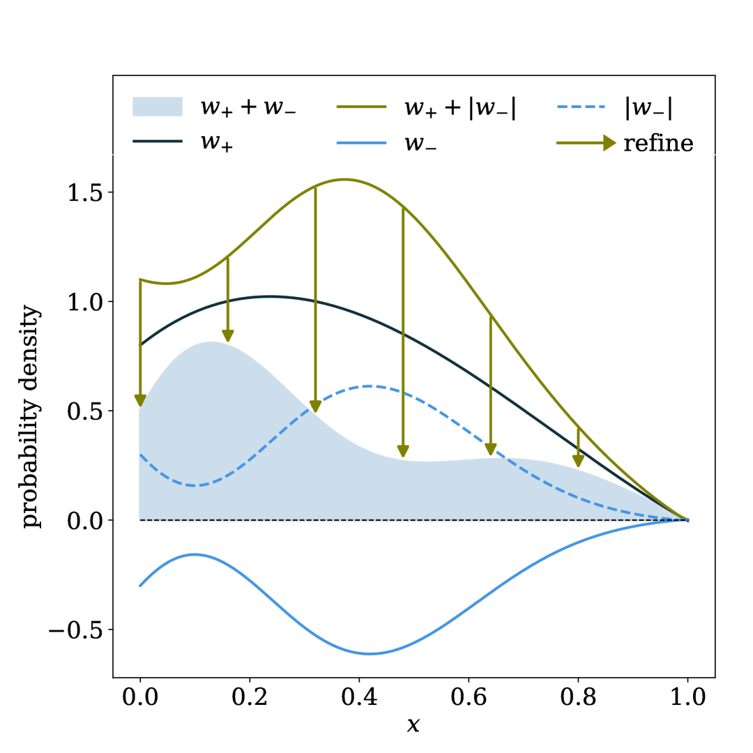
Figure 1: Graphical illustration of the refinement method and the distribution of samples with different weights.

After the refinement, the local resampling strategy introduced in Ref. [9] can be used to restore statistical properties and uncertainties of the samples.

The refinement method offers several potential benefits over reweighting, including:

• Simplified task: The network is only required to learn the refinement between the distributions of pseudo-positive and positive weights. This means that the network does not need to learn the complete normalization and shape of the distribution of positive and negative weights, which can be a more complex task.

• Preservation of weight spectrum: As the refinement factor is a multiplicative factor within a particular phase space bin, the refinement method preserves the relative spectrum of weights among the positive and pseudo-positive weights, respectively, in each phase space bin.

• Improved extrapolation: The refinement method can exhibit better extrapolation to regions where the distribution of weights is non-trivial, but the ratio between pseudo-positive and positive weights is well-behaved and learnable by a neural network.

• Robustness to negative density: The refinement method is resilient to the occurrence of samples from a phase space with a negative density, whereas similar approaches are not and show diverging behavior in these cases. While a negative density is unphysical per se, it can occur in several cases as described below.

Each of these benefits is individually demonstrated in the case studies presented in the next section, providing a comprehensive evaluation of the advantages of the refinement method.

III Case Studies

Several case studies are performed to showcase the working principle of the weight refinement and to illustrate the successful application of the method. As a benchmark, we compare with reweighting, implementing the neural resampling method [9].

In each case study, 80% of the samples are used for training and 20% of the samples are used for testing. The figures involving the evaluation of trained networks show the distributions of samples used for testing only.

All neural networks feature a feed-forward architecture, consisting of two hidden layers with 128 nodes each, and utilize the ReLU activation function. If not noted differently, the networks are trained for 10 epochs with a batch size of 1024 samples using the Adam optimizer with a learning rate decaying exponentially from $10^{-3}$ to $10^{-6}$ during the complete training process. As the reweighter method uses each sample twice in each epoch, once with its original weight and once with a nominal weight, the neural network for the reweighter method is effectively trained on twice the number of samples per epoch [9]. The hyperparameters were not extensively optimized, but small changes in the setup did not result in qualitative changes in performance.

All neural networks used in the case studies were implemented and trained using the TensorFlow [10] and Keras [11] deep learning frameworks.

III.1 Top Quark Pair Production

The first case study shows the performance of the refiner and the reweighter method on a realistic physics dataset with top quark pair production at next-to-leading order (NLO) in quantum chromodynamics (QCD). It is based on a total number of 2M events which were generated as described in Ref. [9] and briefly summarized in the following. Fixed-order matrix elements are generated using MG5_aMC@NLO 5.2.7.2 [12] interfaced with the NNPDF 2.3 NLO parton density function set [13]. These calculations use MadLoop 2.7.2 [14, 12], Ninja 1.2.0 [15, 16], CutTools 1.9.3 [17], and OneLoop 3.6  [18, 19]. Both top quarks decay leptonically via $t\bar{t}\rightarrow b\bar{b}\mu^{+}\mu^{-}\nu\bar{\nu}$. The default FKS subtraction scheme [20, 21], is used to match the resulting samples with the Pythia 8.230 [22, 23] parton shower, with its default settings. The output of Pythia is recorded in the HepMC 2.06.09 [24] format and then processed with Delphes 3.4.2 [25]. The reconstructed particles are then clustered into $R=0.4$ anti-$k_{t}$ jets [26] with FastJet [27]. Jets are $b$-tagged using the flavor tagging module in Delphes.

The dataset consists of events with two charged leptons, two neutrinos, two $b$-jets, and a variable number of additional jets, up to a maximum of 15 objects/event. Each object is characterized by a $p_{T}$, $\eta$, $\phi$, mass, and identification (integer encoding type). Due to the variable number of jets per event, the weight transformation task on this dataset is inherently variable-dimensional. For this example, we simplify the problem by zero padding and then using a fully connected neural network. Architectures naturally able to ingest variable-length inputs may be more efficient, although that was not a challenge in this study. To assess the performance of the methods, 10 independent neural networks with different random initializations are trained for both the reweighting and refinement tasks.

To illustrate the impact of negative weight mitigation in the $t\bar{t}$ example, we examine the charged particle $p_{T}$ spectrum in Figure 2 (the results are similar for other observables). In this example, about 20% of events have negative weights. Figure 2b demonstrates that both reweigthing and refining are able to match the original spectrum with negative weights (labeled ‘Data’). The error bands in the ratio show that both methods are robust to the network initialization, with a spread that is typically smaller than the statistical uncertainty. There is an interplay between this spread and the hyperparameter optimization and it would be interesting to explore this in further detail in the future.

The resulting distribution of weights are presented in Figure 2c. As desired, the reweighted/refined weights are non-negative and have nearly the same distribution since they have the same target. This top quark example shows that on a relevant particle physics problem with a relatively simple weight distribution, both reweighting and refining work well. The next sections focus on synthetic examples that clearly highlight potential advantages of refining over reweighting. While the trends are exaggerated, the accuracy requirements at current and future experiments may be sensitive to scaled down versions of these setups.

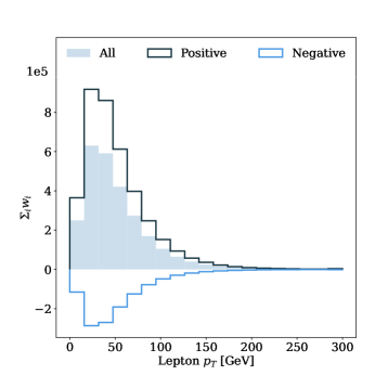
(a)

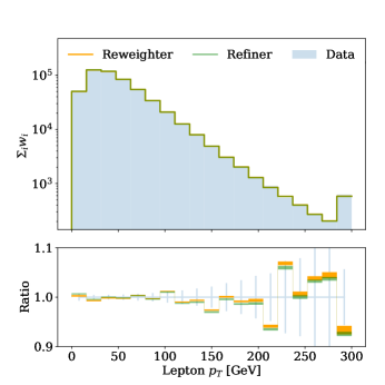
(b)

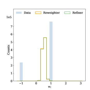
(c)

Figure 2: Top quark pair production. Left: a histogram of the positively charged lepton transverse momentum broken down into positive and negative events. Middle: the reweighted/refined spectrum compared to the initial data (with negative weights). Right: the distribution of event weights before and after reweighting/refining. The error bands in the middle plot represent the spread across the 10 networks and the vertical error bars represent the statistical uncertainty.

III.2 Synthetic Shape Example

This case study compares the performance of the refiner and the reweighter method on a case in which the sample weights follow a non-trivial shape. For illustration, we consider a case where 10M samples are uniformly distributed. Their weights follow a non-differentiable, positive distribution defined by a piecewise function comprising a rectangle, triangle, and inverted quadratic spline as shown in Figure 3a. Since all samples have positive weights, the distribution of positively weighted samples is identical to the overall sample distribution and no weight transformation is required. The refiner approach can exploit this, allowing the network to simply learn the identity function. In contrast, the reweighter approach attempts to infer the entire weight distribution, necessitating the network to learn the non-trivial shape.

Figure 3b and fig. 3c display the distributions of samples and weights before and after the weight transformations, respectively. As anticipated, the refiner approach yields highly accurate sample and weight distributions, since it only requires learning the identity function. In contrast, the sample and weight distributions of the reweighter approach exhibit various artifacts and mismodellings, resulting from the complex, non-trivial distribution of weights, which poses significant challenges for neural network modeling. This study highlights the fact that the weight refinement can be less challenging and more accurate than corresponding methods, depending on the shape of the weights.

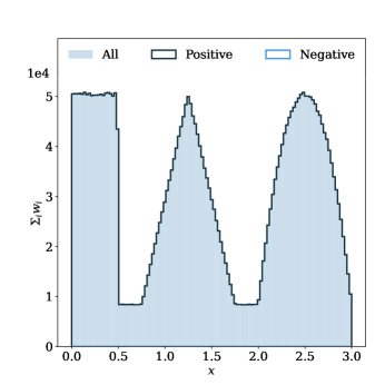
(a)

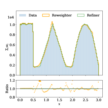
(b)

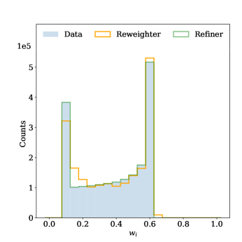
(c)

Figure 3: Non-trivial, non-negative weight distribution. Left: a histogram of the synthetic observable broken down into positive and negative events. Middle: the reweighted/refined spectrum compared to the initial data (with negative weights). Right: the distribution of event weights before and after reweighting/refining. The error bars in the middle plot represent statistical uncertainties.

III.3 Synthetic Spectrum Example

This case study shows the performance of the refiner and the reweighter method on a case in which the weights have a stochastic spread in each particular phase space bin. For illustration, the samples follow a distribution that can be described by two separate Gaussian functions. Additionally, the sample weights within each phase space bin are also distributed according to two Gaussian functions.

In particular, the data consist of 7.5M samples following a Gaussian distribution centered at 0 with a width of 1 with weights following a Gaussian distribution centered at 1 with a spread of 0.2 and 2.5M samples following a Gaussian distribution centered at 0 with a width of 0.5 with weights following a Gaussian distribution centered at -1 with a spread of 0.2. Figure 4a displays the distribution of samples with their original weights prior to the weight transformations and the light-colored points in Figure 4c show the corresponding weight distributions.

Figure 4b demonstrates that both transformations work and can restore the original distribution within the statistical uncertainties. However, Figure 4c shows that the reweighter approach predicts one weight for each phase space bin, while the refiner approach predicts a whole spectrum of weights in each phase space bin. Doing this, the refiner approach preserves the relative spectrum of weights among the positive and pseudo-positive weights, respectively, in each phase space bin. While not necessarily an advantage, it could be useful if downstream analysis makes use of the latent degrees of freedom that produce the stochastic weight distribution.

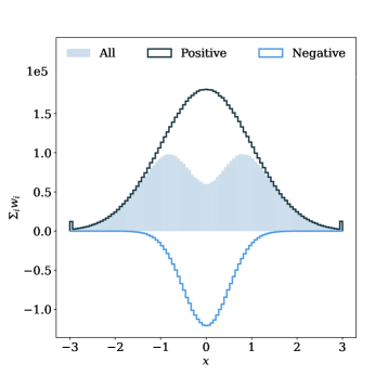
(a)

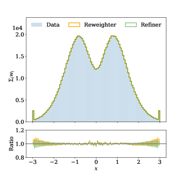
(b)

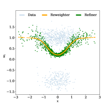
(c)

Figure 4: Gaussian observable with Gaussian weights, including negative weights. Left: a histogram of the synthetic observable broken down into positive and negative events. Middle: the reweighted/refined spectrum compared to the initial data (with negative weights). Right: the distribution of event weights before and after reweighting/refining. The error bars in the middle plot represent statistical uncertainties.

III.4 Synthetic Extrapolation Example

This case study demonstrates the extrapolation capabilities of the reweighter and refiner methods to extend beyond the region where the majority of samples are concentrated and the weight distribution can be readily learned. For illustration, we use the same dataset as in the previous section, but with no spread in weights for the positive and negative weight samples. This allows us to focus on the tails of the distribution to explore the extrapolation properties.

In particular, the data consist of 7.5M samples following a Gaussian distribution centered at 0 with a width of 1 with weights set to 1 and 2.5M samples following a Gaussian distribution centered at 0 with a width of 0.5 with weights set to -1. Figure 5a displays the distribution of samples with their original weights prior to the weight transformations.

Figure 5b displays the sample distributions before and after weight transformations. Both transformations are effective in restoring the original distribution within statistical uncertainties. However, a systematic up-fluctuation is evident on the sides of the distribution for the reweighter approach. This corresponds to a weight function in fig. 5b that increases in both directions away from zero, when it should instead be a constant. This case study demonstrates that the refiner approach can have better extrapolation capabilities than corresponding methods, depending on the shape of the weights.

(a)

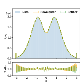
(b)

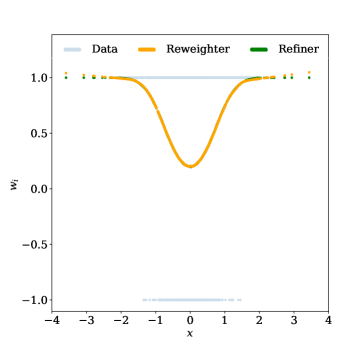
(c)

Figure 5: Gaussian observable with non-random weights, including negative weights. Left: a histogram of the synthetic observable broken down into positive and negative events. Middle: the reweighted/refined spectrum compared to the initial data (with negative weights). Right: the distribution of event weights before and after reweighting/refining. The error bars in the middle plot represent statistical uncertainties.

III.5 Synthetic Negative Density Example

This case study compares the performance of the reweighter and the refiner method on a case in which some part of the phase space has a negative density. While this is not possible for physical cross sections, scenarios with negative sample density can arise in various situations. For instance, limited statistics can lead to negative densities in certain regions of phase space, even if the underlying distribution is non-negative. Additionally, certain analysis techniques may involve non-physical processes with negative cross sections, such as events representing interference terms. Furthermore, the breakdown of perturbation theory near soft/collinear singularities can result in negative cross sections. While issues related to perturbation theory breakdown can be addressed through methods like matching to a parton shower, the refinement approach does not necessarily require such mitigation, as it can handle regions with negative weights without modification.

It is not possible to render all weights non-negative in a phase space region with an overall negative underlying density. However, it should still be possible to apply a weight transformation method to the overall phase space, allowing for a graceful transformation of weights in the remaining phase space. As demonstrated below, the refiner method exhibits this desirable property, in contrast to the reweighter approach.

For illustration, we generate 7.5M samples following a Gaussian distribution centered at 0 with a width of 1 with weights set to 1 and 2M samples following a Gaussian distribution centered at 0 with a width of 0.2 with weights set to -1. Figure 6a displays the distribution of samples with their original weights prior to the weight transformations. It can be seen that the density of the weighted samples is negative in the range from $-0.14$ to $0.14$.

Figure 6b shows the sample distributions before and after the weight transformations. To illustrate the divergent behavior of the reweighter approach, its neural network is deliberately trained using the Adam optimizer with a fixed learning rate of $2\times 10^{-5}$, not hiding its divergent behavior with a decaying learning rate. The refiner approach is able to accurately model the entire distribution, including the region of phase space with negative sample density. In contrast, the reweighter approach, by design, is constrained to produce non-negative weights and therefore fails to capture the distribution in the region of negative density.

Although one might argue that the reweighter’s inability to model negative densities is a desirable feature, the method ultimately fails to adequately capture the remaining part of the phase space. This is because, in the presence of a phase space with negative density, the reweighter becomes overly focused on this region, causing the training loss to diverge negatively, as illustrated in fig. 6c. Even a small fraction of negative phase space can be sufficient to compromise the entire reweighter method. If the network is able to identify this problematic region, the training process will diverge, rendering the reweighter approach unusable. In contrast, the refiner is able to assign negative weights to samples in these regions of phase space and still work properly everywhere else.

This case study demonstrates the resilience of the refiner method in handling phase space regions with negative density, compared to the corresponding reweighter method which does not have this feature.

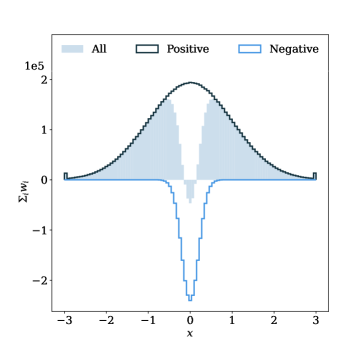
(a)

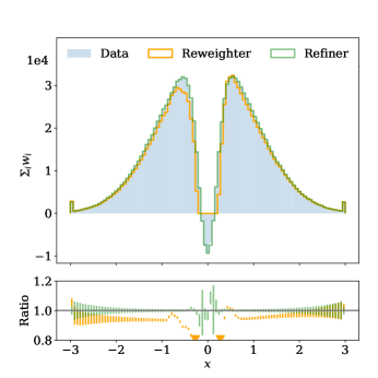
(b)

(c)

Figure 6: Gaussian observable with regions of negative cross section. Left: a histogram of the synthetic observable broken down into positive and negative events. Middle: the reweighted/refined spectrum compared to the initial data (with negative weights). Right: the distribution of event weights before and after reweighting/refining. The error bars in the middle plot represent statistical uncertainties.

IV Conclusion and Outlook

This paper introduces a novel method for transforming sample weights in a weighted dataset, with the goal of rendering them all positive. Our approach scales the original weights of each sample using a phase space dependent refinement factor, offering a simpler learning task compared to previous methods that model the full weight distribution. The paper introduces the method and demonstrates its advantages and comparable or superior performance on multiple physical and synthetic datasets. These advantages include a simplified learning task, preservation of the spectrum of positive and negative weights in each phase space bin, improved extrapolation, and robustness to phase space regions with negative density. While the improvements on current datasets are modest, they might be particularly relevant in the context of increasingly stringent demands on accuracy and precision of simulations in future experiments.

Even though we have focused on cross sections, the refining methodology may be useful more generally when datasets have negative weights. Beyond the task of transforming sample weights, this work also illustrates the importance of considering alternative strategies for likelihood-free inference even when all strategies have the same formal, asymptotic behavior.

Code Availability

The code for this project is available at: https://github.com/Nollde/weight_refiner. The top quark datasets used in this study are available upon request to the authors.

References

- [1] K. Danziger, S. Höche, and F. Siegert, Reducing negative weights in Monte Carlo event generation with Sherpa, arXiv:2110.15211.
- [2] S. Alioli, P. Nason, C. Oleari, and E. Re, A general framework for implementing NLO calculations in shower Monte Carlo programs: the POWHEG BOX, JHEP 06 (2010) 043, [arXiv:1002.2581].
- [3] R. Frederix, S. Frixione, S. Prestel, and P. Torrielli, On the reduction of negative weights in MC@NLO-type matching procedures, JHEP 07 (2020) 238, [arXiv:2002.12716].
- [4] J. R. Andersen, C. Gütschow, A. Maier, and S. Prestel, A Positive Resampler for Monte Carlo events with negative weights, Eur. Phys. J. C 80 (2020), no. 11 1007, [arXiv:2005.09375].
- [5] B. Nachman and J. Thaler, Neural resampler for Monte Carlo reweighting with preserved uncertainties, Phys. Rev. D 102 (2020), no. 7 076004, [arXiv:2007.11586].
- [6] J. R. Andersen and A. Maier, Unbiased elimination of negative weights in Monte Carlo samples, Eur. Phys. J. C 82 (2022), no. 5 433, [arXiv:2109.07851].
- [7] J. R. Andersen, A. Maier, and D. Maître, Efficient negative-weight elimination in large high-multiplicity Monte Carlo event samples, Eur. Phys. J. C 83 (2023), no. 9 835, [arXiv:2303.15246].
- [8] J. R. Andersen, A. Cueto, S. P. Jones, and A. Maier, A Cell Resampler study of Negative Weights in Multi-jet Merged Samples, arXiv:2411.11651.
- [9] B. Nachman and J. Thaler, Neural resampler for monte carlo reweighting with preserved uncertainties, Physical Review D 102 (Oct., 2020).
- [10] M. Abadi, A. Agarwal, P. Barham, E. Brevdo, Z. Chen, C. Citro, G. S. Corrado, A. Davis, J. Dean, M. Devin, S. Ghemawat, I. Goodfellow, A. Harp, G. Irving, M. Isard, Y. Jia, R. Jozefowicz, L. Kaiser, M. Kudlur, J. Levenberg, D. Mané, R. Monga, S. Moore, D. Murray, C. Olah, M. Schuster, J. Shlens, B. Steiner, I. Sutskever, K. Talwar, P. Tucker, V. Vanhoucke, V. Vasudevan, F. Viégas, O. Vinyals, P. Warden, M. Wattenberg, M. Wicke, Y. Yu, and X. Zheng, TensorFlow: Large-scale machine learning on heterogeneous systems, 2015. Software available from tensorflow.org.
- [11] F. Chollet et al., “Keras.” https://keras.io, 2015.
- [12] J. Alwall, R. Frederix, S. Frixione, V. Hirschi, F. Maltoni, O. Mattelaer, H. S. Shao, T. Stelzer, P. Torrielli, and M. Zaro, The automated computation of tree-level and next-to-leading order differential cross sections, and their matching to parton shower simulations, JHEP 07 (2014) 079, [arXiv:1405.0301].
- [13] R. D. Ball et al., Parton distributions with LHC data, Nucl. Phys. B 867 (2013) 244–289, [arXiv:1207.1303].
- [14] V. Hirschi, R. Frederix, S. Frixione, M. V. Garzelli, F. Maltoni, and R. Pittau, Automation of one-loop QCD corrections, JHEP 05 (2011) 044, [arXiv:1103.0621].
- [15] P. Mastrolia, E. Mirabella, and T. Peraro, Integrand reduction of one-loop scattering amplitudes through Laurent series expansion, JHEP 06 (2012) 095, [arXiv:1203.0291]. [Erratum: JHEP 11, 128 (2012)].
- [16] T. Peraro, Ninja: Automated Integrand Reduction via Laurent Expansion for One-Loop Amplitudes, Comput. Phys. Commun. 185 (2014) 2771–2797, [arXiv:1403.1229].
- [17] G. Ossola, C. G. Papadopoulos, and R. Pittau, CutTools: A Program implementing the OPP reduction method to compute one-loop amplitudes, JHEP 03 (2008) 042, [arXiv:0711.3596].
- [18] A. van Hameren, OneLOop: For the evaluation of one-loop scalar functions, Comput. Phys. Commun. 182 (2011) 2427–2438, [arXiv:1007.4716].
- [19] A. van Hameren, C. Papadopoulos, and R. Pittau, Automated one-loop calculations: A Proof of concept, JHEP 09 (2009) 106, [arXiv:0903.4665].
- [20] S. Frixione, Z. Kunszt, and A. Signer, Three jet cross-sections to next-to-leading order, Nucl. Phys. B 467 (1996) 399–442, [hep-ph/9512328].
- [21] S. Frixione, A General approach to jet cross-sections in QCD, Nucl. Phys. B 507 (1997) 295–314, [hep-ph/9706545].
- [22] T. Sjöstrand, S. Ask, J. R. Christiansen, R. Corke, N. Desai, P. Ilten, S. Mrenna, S. Prestel, C. O. Rasmussen, and P. Z. Skands, An Introduction to PYTHIA 8.2, Comput. Phys. Commun. 191 (2015) 159–177, [arXiv:1410.3012].
- [23] T. Sjöstrand, S. Mrenna, and P. Z. Skands, PYTHIA 6.4 Physics and Manual, JHEP 05 (2006) 026, [hep-ph/0603175].
- [24] M. Dobbs and J. B. Hansen, The HepMC C++ Monte Carlo Event Record for High Energy Physics, Tech. Rep. ATL-SOFT-2000-001, CERN, Geneva, Jun, 2000. revised version number 1 submitted on 2001-02-27 09:54:32.
- [25] DELPHES 3 Collaboration, J. de Favereau, C. Delaere, P. Demin, A. Giammanco, V. Lemaître, A. Mertens, and M. Selvaggi, DELPHES 3, A modular framework for fast simulation of a generic collider experiment, JHEP 02 (2014) 057, [arXiv:1307.6346].
- [26] M. Cacciari, G. P. Salam, and G. Soyez, FastJet User Manual, Eur. Phys. J. C72 (2012) 1896, [arXiv:1111.6097].
- [27] M. Cacciari and G. P. Salam, Dispelling the myth for the jet-finder, Phys. Lett. B641 (2006) 57–61, [hep-ph/0512210].