Transformers for Learning on Noisy and Task-Level Manifolds: Approximation and Generalization Insights

Abstract

Transformers serve as the foundational architecture for large language and video generation models, such as GPT, BERT, SORA and their successors. Empirical studies have demonstrated that real-world data and learning tasks exhibit low-dimensional structures, along with some noise or measurement error. The performance of transformers tends to depend on the intrinsic dimension of the data/tasks, though theoretical understandings remain largely unexplored for transformers. This work establishes a theoretical foundation by analyzing the performance of transformers for regression tasks involving noisy input data on a manifold. Specifically, the input data are in a tubular neighborhood of a manifold, while the ground truth function depends on the projection of the noisy data onto the manifold. We prove approximation and generalization errors which crucially depend on the intrinsic dimension of the manifold. Our results demonstrate that transformers can leverage low-complexity structures in learning task even when the input data are perturbed by high-dimensional noise. Our novel proof technique constructs representations of basic arithmetic operations by transformers, which may hold independent interest.

1 Introduction

Transformer architecture, introduced in Vaswani et al. [2017], has reshaped the landscape of machine learning, enabling unprecedented advancements in natural language processing (NLP), computer vision, and beyond. In transformers, traditional recurrent and convolutional architectures are replaced by an attention mechanism. Transformers have achieved remarkable success in large language models (LLMs) and video generation, such as GPT [Achiam et al., 2023], BERT [Devlin, 2018], SORA [Brooks et al., 2024] and their successors.

Despite the success of transformers, their approximation and generalization capabilities remain less explored compared to other network architectures, such as feedforward and convolutional neural networks. Some theoretical investigations of transformers can be found in Jelassi et al. [2022]; Yun et al. [2019]; Edelman et al. [2022]; Wei et al. [2022]; Takakura and Suzuki [2023]; Gurevych et al. [2022]; Bai et al. [2023]. Specifically, Yun et al. [2019] proved that transformer models can universally approximate continuous sequence-to-sequence functions on a compact support, while while the network size grows exponentially with respect to the sequence dimension. Edelman et al. [2022] evaluated the capacity of Transformer networks and derived the sample complexity to learn sparse Boolean functions. Takakura and Suzuki [2023] studied the approximation and estimation ability of Transformers as sequence-to-sequence functions with anisotropic smoothness on infinite dimensional input. Gurevych et al. [2022] studied binary classification with transformers when the posterior probability function exhibits a hierarchical composition model with Hölder smoothness. Jelassi et al. [2022] analyzed a simplified version of vision transformers and showed that they can learn the spatial structure and generalize. Lai et al. [2024] established a connection between transformers and smooth cubic splines. Bai et al. [2023] proved the in-context learning ability of transformers for least squares, ridge regression, Lasso and generalized linear models.

Compared to transformers, feedforward and convolutional neural networks are significantly better understood in terms of approximation [Cybenko, 1989; Hornik et al., 1989; Leshno et al., 1993; Mhaskar, 1993; Bach, 2017; Maiorov, 1999; Pinkus, 1999; Petrushev, 1998; Yarotsky, 2017; Lu et al., 2021; Oono and Suzuki, 2019; Lai and Shen, 2021, 2024; Zhou, 2020] and generalization [Kohler and Mehnert, 2011; Schmidt-Hieber, 2020; Oono and Suzuki, 2019] theories. Theoretical results in Yarotsky [2017]; Lu et al. [2021]; Oono and Suzuki [2019]; Schmidt-Hieber [2020] addressed function approximation and estimation in a Euclidean space. For functions supported on a low-dimensional manifold, approximation and generalization theories were established for feedforward neural networks in Chui and Mhaskar [2018]; Shaham et al. [2018]; Chen et al. [2019]; Schmidt-Hieber [2019]; Nakada and Imaizumi [2020]; Chen et al. [2022] and for convolutional residual neural networks in Liu et al. [2021]. To relax the exact manifold assumption and allow for noise on input data, Cloninger and Klock [2021] studied approximation properties of feedforward neural networks under inexact manifold assumption, i.e., data are in a tubular neighborhood of a manifold and the groundtruth function depends on the projection of the noisy data onto the manifold. This relaxation accommodates input data with noise and accounts for the low complexity of the learning task beyond the low intrinsic dimension of the input data, making the theory applicable to a wider range of practical scenarios for feedforward neural networks.

In the application of transformers, empirical studies have demonstrated that image, video, text data and learning tasks tend to exhibit low-dimensional structures [Pope et al., 2021; Sharma and Kaplan, 2022; Havrilla and Liao, 2024], along with some noise or measurement error in real-world data sets. The performance of transformers tends to depend on the intrinsic dimension of the data/tasks [Sharma and Kaplan, 2022; Havrilla and Liao, 2024; Razzhigaev et al., 2023; Min et al., 2023; Aghajanyan et al., 2020]. Specifically, Aghajanyan et al. [2020] empirically showed that common pre-trained models in NLP have a very low intrinsic dimension. Pope et al. [2021]; Razzhigaev et al. [2023]; Havrilla and Liao [2024] investigated the intrinsic dimension of token embeddings in transformer architectures, and obtained a significantly lower intrinsic dimension than the token dimension.

Despite of the empirical findings connecting to performance of transformers with the low intrinsic dimension of data/tasks, theoretical understandings about how transformers adapt to low-dimensional data/task structures and build robust predictions against noise are largely open. Havrilla and Liao [2024] analyzed the approximation and generalization capability of transformers for regression tasks when the input data exactly lie on a low-dimensional manifold. However, the setup in Havrilla and Liao [2024] does not account for noisy data concentrated near a low-dimensional manifold and low-complexity in the regression function.

In this paper, we bridge this theoretical gap by analyzing the approximation and generalization error of transformers for regression of functions on a tubular neighborhood of a manifold. To leverage the low-dimensional structures in the learning task, the function depends on the projection of the input onto the manifold. Specifically, let $\mathcal{M}\subseteq[0,1]^{D}$ be a compact, connected $d$-dimensional Riemannian manifold isometrically embedded in $\mathbb{R}^{D}$ with a positive reach $\tau_{\mathcal{M}}$, and $\mathcal{M}(q)$ be a tubular region around the manifold $\mathcal{M}$ with local tube radius given by $q\in[0,1)$ times the local reach (see Definitions 1 and 4). We consider function $f:\mathcal{M}(q)\to\mathbb{R}$ in the form:

$$f(x)=g(\pi_{\mathcal{M}}(x)),\ \ \forall x\in\mathcal{M}(q)$$ (1)

where

$$\pi_{\mathcal{M}}(x)=\operatorname*{arg\,min}_{z\in\mathcal{M}}\|x-z\|_{2},$$ (2)

is the orthogonal projection onto the manifold $\mathcal{M}$, and $g:\mathcal{M}\to\mathbb{R}$ is an unknown $\alpha$-Hölder function on the manifold $\mathcal{M}$. An illustration of the tubular region and the orthogonal projection onto the manifold is shown in Figure 1.

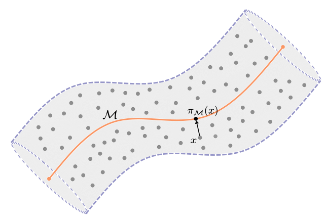
Figure 1: The tubular region around manifold $\mathcal{M}$ and the orthogonal projection $\pi_{\mathcal{M}}$.

The regression model in (1) covers a variety of interesting scenarios: 1) Noisy Input Data: The input $x$ is a perturbation of its clean counterpart $\pi_{\mathcal{M}}(x)$ on the manifold $\mathcal{M}$. One can access the input and output pairs, i.e. $(x,f(x))$ but the clean counterpart $\pi_{\mathcal{M}}(x)$ is not available in this learning task. 2) Low Intrinsic Dimension in the Machine Learning Task: The input data live in a high-dimensional space $\mathbb{R}^{D}$, but the regression or inference task has a low complexity. In other words, the output $f(x)$ locally depends on $d$ tangential directions on the task manifold $\mathcal{M}$, and the function is locally invariant along the $D-d$ normal directions on the manifold. The model in (1) is also general enough to include many interesting special cases. For example, when $\mathcal{M}$ is a linear subspace, the model in (1) becomes the well-known multi-index model [Cook and Li, 2002]. When $q=0$, one recovers the exact manifold regression model where functions are supported exactly on a low-dimensional manifold.

In this paper, we establish novel mathematical approximation and statistical estimation (or generalization) theories for functions in (1) via transformer neural networks.
Approximation Theory: Under proper assumptions of $\mathcal{M}$, for any $\epsilon>0$, there exists a transformer neural network to universally approximate function $f$ in (1) up to $\epsilon$ accuracy (Theorem 1). The width of this transformer network is in the order of $D\epsilon^{-\frac{d}{\alpha}}$ and the depth is in the order of $d+\ln(\ln(\epsilon^{-1}))$. Note that $d$ is the intrinsic dimension of the manifold $\mathcal{M}$ and $\alpha$ represents the Hölder smoothness of $g$. In this result, the network complexity crucially depends on the intrinsic dimension.
Generalization Theory: When $n$ i.i.d. training samples $\{(x_{i},f(x_{i}))\}_{i=1}^{n}$ are given, we consider the empirical risk minimizer $\hat{\rm T}$ to be defined in (10). Theorem 2 shows that the squared generalization error of $\hat{\rm T}$ is upper bounded in the order of $n^{-\frac{2\alpha}{2\alpha+d}}$. In the exact manifold case when $q=0$, Theorem 2 gives rise to the min-max regression error [Györfi et al., 2006]. In the noisy case when $q\in(0,1)$, Theorem 2 demonstrates a denoising phenomenon given by transformers such that when the sample size $n$ increases, the generalization error converges to $0$ at a fast rate depending on the intrinsic dimension $d$.
Basic Arithmetic Operations Implemented by Transformers: In addition, our proof explicitly constructs transformers to implement basic arithmetic operations, such as addition, constant multiplication, product, division, etc. Such implementation can be done efficiently (e.g., in parallel) on different tokens. These results can be applied individually as building blocks for approximation studies using Transformers.

This paper is organized as follows. In section 2, we introduce some preliminary definitions. In section 3, we present our main results, including the approximation and generalization error bound achieved by transformer networks. In section 4, we provide a proof sketch of our main results. In Section 6, we make conclusion and discuss its impact.

2 Preliminaries

2.1 Manifold

Definition 1 (Manifold)

An $d$-dimensional manifold $\mathcal{M}$ is a topological space where each point has a neighborhood that is homeomorphic to an open subset of $\mathbb{R}^{d}$. Further, distinct points in $\mathcal{M}$ can be separated by disjoint neighborhoods, and $\mathcal{M}$ has a countable basis for its topology.

Definition 2 (Medial Axis)

Let $\mathcal{M}\subseteq\mathbb{R}^{D}$ be a connected and compact $d$-dimensional submanifold. Its medial axis is defined as

$$\begin{split}\text{Med}(\mathcal{M}):=\{x\in\mathbb{R}^{D}\text{ }|&\text{ }\exists p\neq q\in\mathcal{M},\|p-x\|_{2}=\|q-x\|_{2}=\inf_{z\in\mathcal{M}}\|z-x\|_{2}\},\end{split}$$

which contains all points $x\in\mathbb{R}^{D}$ with set-valued orthogonal projection $\pi_{\mathcal{M}}(x)=\operatorname*{arg\,min}_{z\in\mathcal{M}}\|x-z\|_{2}$.

Definition 3 (Local Reach and Reach of a Manifold)

The local reach for $v\in\mathcal{M}$ is defined as $\tau_{\mathcal{M}}(v):=\inf_{z\in\text{Med}(\mathcal{M})}\|v-z\|_{2},$ which describes the minimum distance needed to travel from $v$ to the closure of medial axis. The smallest local reach $\tau_{\mathcal{M}}:=\inf_{v\in\mathcal{M}}\tau_{\mathcal{M}}(v)$ is called reach of $\mathcal{M}$.

Definition 4 (Tubular Region around a Manifold)

Let $q\in[0,1)$. The tubular region around the manifold $\mathcal{M}$ with local tube radius $q\tau_{\mathcal{M}}(v)$ is defined as

$$\mathcal{M}(q):=\{x\in\mathbb{R}^{D}\text{ }| \text{ }x=v+u,v\in\mathcal{M},u\in ker(P(v)^{\top}),$$

$$\|u\|_{2}<q\tau_{\mathcal{M}}(v)\},$$ (3)

where the columns of $P(v)\in\mathbb{R}^{D\times d}$ represent an orthonormal basis of the tangent space of $\mathcal{M}$ at $v$.

Definition 5 (Geodesic Distance)

The geodesic distance between $v,v^{\prime}\in\mathcal{M}$ is defined as

$$d_{\mathcal{M}}(v,v^{\prime}):=\inf\{|\gamma|: \gamma\in C^{1}([t,t^{\prime}]),\gamma:[t,t^{\prime}]\to\mathcal{M},$$

$$\gamma(t)=v,\gamma(t^{\prime})=v^{\prime}\},$$

where the length is defined by $|\gamma|:=\int_{t}^{t^{\prime}}\|\gamma^{\prime}(s)\|_{2}ds$. The existence of a length-minimizing geodesic $\gamma:[t,t^{\prime}]\to\mathcal{M}$ between any two points $v=\gamma(t),v^{\prime}=\gamma(t^{\prime})$ is guaranteed by Hopf–Rinow theorem [Hopf and Rinow, 1931].

Definition 6 ($\delta$-Separated and Maximal Separated Set)

Let $S$ be a set associated with a metric $d$, we say $Z\subseteq S$ is $\delta$-separated if for any $z,z^{\prime}\in Z$, we have $d(z,z^{\prime})>\delta$. We say $Z\subseteq S$ is maximal separated $\delta$-net if adding another point in $Z$ destroys the $\delta$-separated property.

Definition 7 (Covering Number)

Let $(\mathcal{H},\rho)$ be a metric space, where $\mathcal{H}$ is the set of objects and $\rho$ is a metric. For a given $\epsilon>0$, the covering number $\mathcal{N}(\epsilon,\mathcal{H},\rho)$ is the smallest number of balls of radius $\epsilon$ (with respect to $\rho$) needed to cover $\mathcal{H}$. More precisely,

$$\mathcal{N}(\epsilon,\mathcal{H},\rho):=\min\{N\in\mathbb{N}\text{ }|\text{ }\exists\{h_{1},h_{2},\dots,h_{N}\}\subseteq\mathcal{H},$$

$$\quad\quad\quad\quad\quad\quad\quad\quad\ \forall h\in\mathcal{H},\ \exists h_{i}\text{ such that }\rho(h,h_{i})\leq\epsilon\}.$$

Let $d_{\mathcal{M}}$ be a geodesic metric defined on $\mathcal{M}$, we can extend $d_{\mathcal{M}}$ to the tubular region $\mathcal{M}(q)$ such that

$$d_{\mathcal{M}(q)}(u,v):=d_{\mathcal{M}}(\pi_{\mathcal{M}}(u),\pi_{\mathcal{M}}(v)),$$

provided that $u,v\in\mathcal{M}(q)$ has the unique orthogonal projection onto $\mathcal{M}$. According to Cloninger and Klock [2021, Lemma 2.1], for any $x\in\mathcal{M}(q)$ with $q\in[0,1)$, $x$ has a unique projection onto $\mathcal{M}$ such that $\pi_{\mathcal{M}}(x)=v$.

2.2 Transformer Network Class

Definition 8 (Feed-forward Network Class)

The feed-forward neural network (FFN) class with weights $\theta$ is

$$\mathcal{FFN}(L_{\rm FFN}, w_{\rm FFN})=\{{\rm FFN}(\theta;\cdot)\text{ }|\text{ }{\rm FFN}(\theta;\cdot)\text{ }\text{is a FNN}\text{ with at most }L_{\rm FFN}\text{ }\text{layers and width}\text{ }w_{\rm FFN}\}.$$

We use ReLU function $\sigma(x)=\max(x,0)$ as the activation function in the feed-forward network. Note that each feed-forward layer is applied tokenwise to an embedding matrix $H$.

Definition 9 (Attention and Multi-head Attention)

The attention with the query, key, value matrices $Q,K,V\in\mathbb{R}^{d_{embed}\times d_{embed}}$ is

$$\textstyle A_{K,Q,V}(H)=VH\sigma((KH)^{\top}QH).$$ (4)

It is worthwhile to note that the following formulation is convenient when analyzing the interaction between a pair of tokens, which is more relevant to us.

$$\textstyle A(h_{i})=\sum_{i=1}^{\ell}\sigma(\langle Qh_{i},Kh_{j}\rangle)Vh_{j}$$ (5)

The multi-head attention (MHA) with $m$ heads is

$$\textstyle{\rm MHA}(H)=\sum_{j=1}^{m}V_{j}H\sigma((K_{j}H)^{\top}Q_{j}H).$$ (6)

Note that in this paper, we consider ReLU as the activation function rather than Softmax in the attention.

Definition 10 (Transformer Block)

The transformer block is a residual composition of the form

$${\rm B}(H)={\rm FFN}({\rm MHA}(H)+H)+{\rm MHA}(H)+H.$$ (7)

Definition 11 (Transformer Block Class)

The transformer block class with weights $\theta$ is

$$\mathcal{B}(m,L_{\rm FFN},w_{\rm FFN})=\{{\rm B}(\theta;\cdot)\text{ }| \text{ }{\rm B}(\theta;\cdot)\text{ }\text{a {\rm MHA} with }m\text{ attention heads, and a {\rm FNN} layer }$$

$$\text{with depth }L_{\rm FFN}\text{ }\text{and width }w_{\rm FFN}\}.$$

Definition 12 (Transformer Network)

A transformer network $T(\theta;\cdot)$ with weights $\theta$ is a composition of an embedding layer, a positional encoding matrix, a sequence transformer blocks, and a decoding layer, i.e.,

$${\rm T}(\theta;x):={\rm DE}\circ{\rm B}_{L_{T}}\circ\cdots\circ{\rm B}_{1}\circ({\rm PE}+{\rm E}(x)),$$ (8)

where $x\in\mathbb{R}^{D}$ is the input, ${\rm E}:\mathbb{R}^{D}\to\mathbb{R}^{d_{embed}\times\ell}$ is the linear embedding, ${\rm PE}\in\mathbb{R}^{d_{embed}\times\ell}$ is the positional encoding. ${\rm B}_{1},\cdots,{\rm B}_{L_{T}}:\mathbb{R}^{d_{embed}\times\ell}\to\mathbb{R}^{d_{embed}\times\ell}$ are the transformer blocks where each block consists of the residual composition of multi-head attention layers and feed-forward layers. ${\rm DE}:\mathbb{R}^{d_{embed}\times\ell}\to\mathbb{R}$ is the decoding layer which outputs the first element in the last column.

In our analysis, we utilize the well-known sinusoidal positional encoding $\mathcal{I}_{j}\in\mathbb{R}^{2}$, which can be interpreted as rotations of a unit vector $e_{1}$ within the first quadrant of the unit circle. More precisely, for an embedding matrix $H={\rm PE}+{\rm E}(x)$ given in (13), the first two rows are the data terms, which are used to approximate target function. The third and fourth rows are interaction terms with $\mathcal{I}_{j}=(\cos(\frac{j\pi}{2\ell}),\sin(\frac{j\pi}{2\ell}))^{\top}$, determining when each token embedding will interact with another in the attention mechanism, where $\ell$ is the number of hidden tokens. The last (fifth) row are constant terms.

Definition 13 (Transformer Network Class)

The transformer network class with weights $\theta$ is

$$\mathcal{T}(L_{T},m_{T},d_{embed},\ell,L_{\text{FFN}},w_{\text{FFN}},R,\kappa)$$

$$=\Big{\{}{\rm T}(\theta;\cdot)\text{ }|\text{ }{\rm T}(\theta;\cdot)\text{ has the form }(\ref{Trep})\text{ with }L_{T}\text{ transformer blocks, }\text{at most }m_{T}\text{ attention heads in}$$

$$\quad\quad\quad\quad\quad\quad\text{each block, embedded dimension }d_{embed},\text{number of hidden tokens }\ell,\text{and }L_{\text{FFN}}\text{ layers}$$

$$\quad\quad\quad\quad\quad\quad\text{of feed-forward networks with}\text{ hidden width }w_{\text{FFN}},\text{ with output }\|{\rm T}(\theta;\cdot)\|_{L^{\infty}(\mathbb{R}^{D})}\leq R$$

$$\quad\quad\quad\quad\quad\quad\text{and weight magnitude }\|\theta\|_{\infty}\leq\kappa\Big{\}}.$$

Here $\|\theta\|_{\infty}$ represent the maximum magnitude of the network parameters. When there is no ambiguity in the context, we will shorten the notation $\mathcal{T}(L_{T},m_{T},d_{embed},\ell,L_{\rm FFN},w_{\rm FFN},R,\kappa)$ as $\mathcal{T}$. Throughout the paper, we use $x=(x^{1},\cdots,x^{D})$ as the input variable , with each $x^{i}$ being the $i$-th component of $x$. We summarize the notations in Table 2 in the Appendix A.

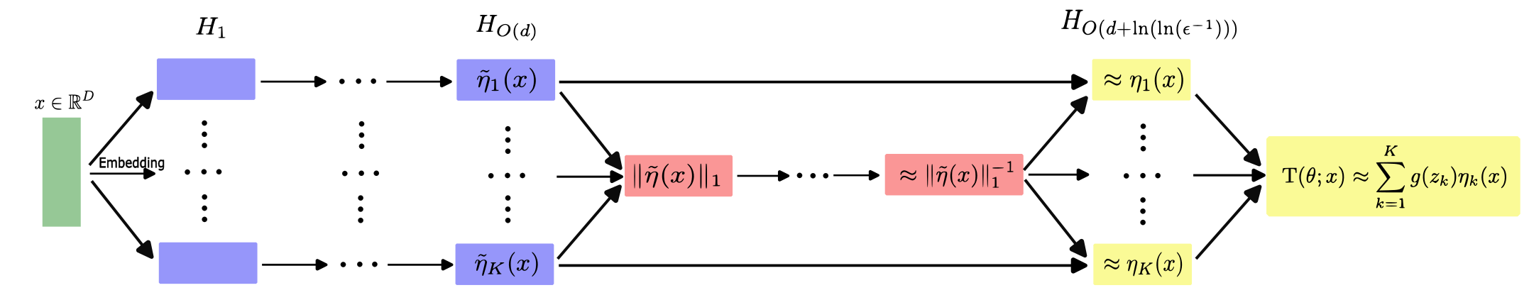
Figure 2: Transformer architecture constructed to approximate $\hat{f}$ (the purple component implements each of the $\tilde{\eta}_{i}$, the red component approximates $\frac{1}{\|\tilde{\eta}\|_{1}}$, the yellow component approximates each of the $\eta_{i}(x)$, and then approximates $\hat{f}$).

3 Transformer Approximation and Generalization Theory

We next present our main results about approximation and generalization theories for estimating functions in (1).

3.1 Assumptions

Assumption 1 (Manifold)

Let $\mathcal{M}\subseteq[0,1]^{D}$ be a non-empty, compact, connected $d$-dimensional Riemannian manifold isometrically embedded in $\mathbb{R}^{D}$ with a positive reach $\tau_{\mathcal{M}}>0$. The tubular region $\mathcal{M}(q)$ defined in (3) satisfies $q\in[0,1)$ and $\mathcal{M}(q)\subseteq[0,1]^{D}$.

Assumption 2 (Target function)

The target function $f:\mathcal{M}(q)\to\mathbb{R}$ can be written in (1) such that $f:=g\circ\pi_{\mathcal{M}}$ and $g:\mathcal{M}\to\mathbb{R}$ is $\alpha$-Hölder continuous with Hölder exponent $\alpha\in(0,1]$ and Hölder constant $L>0$:

$$|g(z)-g(z^{\prime})|\leq Ld^{\alpha}_{\mathcal{M}}(z,z^{\prime})\text{ }\text{ }\text{for all}\text{ }\text{ }z,z^{\prime}\in\mathcal{M}.$$

In addition, we assume $\|f\|_{L^{\infty}(\mathcal{M}(q))}\leq R$ for some $R>0$.

3.2 Transformer Approximation Theory

Our first contribution is a universal approximation theory for functions satisfying Assumption 2 by a transformer network.

Theorem 1

Suppose Assumption 1 holds. For any $\epsilon\in(0,\min\{1,(\tau_{\mathcal{M}}/2)^{\alpha}\})$, there exists a transformer network ${\rm T}(\theta;\cdot)\in\mathcal{T}(L_{\rm T},m_{\rm T},d_{embed},\ell,L_{\rm FFN},w_{\rm FFN},R,\kappa)$ with parameters

$$L_{\rm T}=O(d+\ln(\ln(\epsilon^{-1}))),\text{ }m_{\rm T}=O(D\epsilon^{-\frac{d}{\alpha}}),\text{ }d_{embed}=O(1),$$

$$\ell=O(D\epsilon^{-\frac{d}{\alpha}}),\text{ }L_{\rm FFN}=O(1),\text{ }w_{\rm FFN}=O(1),\text{ }\kappa=O(D^{2}\epsilon^{-\frac{2d+8}{\alpha}})$$

such that, for any $f$ satisfying Assumption 2, if the network parameters $\theta$ are properly chosen, the network yields a function ${\rm T}(\theta;\cdot)$ with

$$\|{\rm T}(\theta;\cdot)-f\|_{\mathcal{L}^{\infty}(\mathcal{M}(q))}\leq\epsilon.$$ (9)

The notation $O(\cdot)$ in $m_{T}$, $\ell$, $\kappa$ hide terms dependent on $d,q,\tau_{\mathcal{M}},L,R,\text{Vol}(\mathcal{M})$, while $O(\cdot)$ in others hide the terms dependent on $q,\tau_{\mathcal{M}},L,R,\text{Vol}(\mathcal{M})$.

The proof of Theorem 1 is provided in Section 4 and a flow chat of our transformer network is illustrated in Figure 2. One notable feature of Theorem 1 is that the network is shallow. It only requires near constant depth $O(d+\ln(\ln(\epsilon^{-1})))$ to approximate the function $f$ defined on the noisy manifold with any accuracy $\epsilon$. This highlights a key advantage of Transformers over feed-forward ReLU networks, which require substantially more layers, e.g., $O(\ln(\frac{1}{\epsilon}))$, to achieve the same accuracy [Yarotsky, 2017].

3.3 Transformer Generalization Theory

Theorem 1 focuses on the existence of a transformer network class which universally approximates all target functions satisfying Assumption 2. However, it does not yield a computational strategy to obtain the network parameters for any specific function. In practice, the network parameters are obtained by an empirical risk minimization.

Suppose $\{x_{i}\}_{i=1}^{n}$ are $n$ i.i.d samples from a distribution $P$ supported on $\mathcal{M}(q)$, and their corresponding function values are $\{f(x_{i})\}_{i=1}^{n}$. Given $n$ training samples $\{(x_{i},f(x_{i}))\}_{i=1}^{n}$, we consider the empirical risk minimizer $\hat{\rm T}_{n}$ such that

$$\textstyle\hat{\rm T}_{n}:=\operatorname*{arg\,min}_{\rm T\in\mathcal{T}}\frac{1}{n}\sum_{i=1}^{n}({\rm T}(x_{i})-f(x_{i}))^{2},$$ (10)

where $\mathcal{T}$ is a transformer network class. The squared generalization error of $\hat{\rm T}_{n}$ is

$$\mathbb{E}\|\hat{\rm T}_{n}-f\|^{2}_{L^{2}(P)}=\mathbb{E}\int_{\mathcal{M}(q)}(\hat{\rm T}_{n}(x)-f(x))^{2}dP,$$ (11)

where the expectation is taken over $\{x_{i}\}_{i=1}^{n}$.

Our next result establishes a generalization error bound for the regression of $f$.

Theorem 2

Suppose Assumptions 1 and 2 hold. Let $\{(x_{i},f(x_{i}))\}_{i=1}^{n}$ are $n$ training samples where $\{x_{i}\}_{i=1}^{n}$ are $n$ i.i.d samples of a distribution $P$ supported on $\mathcal{M}(q)$. If the transformer network class $\mathcal{T}(L_{\rm T},m_{\rm T},d_{embed},\ell,L_{\rm FFN},w_{\rm FFN},R,\kappa)$ has parameters

$$L_{\rm T}=O(d+\ln(\ln(n^{\frac{\alpha}{2\alpha+d}}))),\text{ }m_{\rm T}=O(Dn^{\frac{d}{2\alpha+d}}),\text{ }d_{embed}=O(1),$$

$$\ell=O(Dn^{\frac{d}{2\alpha+d}}),\text{ }L_{\rm FFN}=O(1),\text{ }w_{\rm FFN}=O(1),\text{ }\kappa=O(D^{2}n^{\frac{2d+8}{2\alpha+d}})$$

where the $O(\cdot)$ in $m_{T}$, $\ell$, $\kappa$ hide terms dependent on $d,q,\tau_{\mathcal{M}},L,R,\text{Vol}(\mathcal{M})$, while $O(\cdot)$ in others hide the terms dependent on $q,\tau_{\mathcal{M}},L,R,\text{Vol}(\mathcal{M})$. Then the empirical risk minimizer $\hat{\rm T}_{n}$ given by (10) satisfies

$$\mathbb{E}\|\hat{\rm T}_{n}-f\|^{2}_{L^{2}(P)}\leq\tilde{O}\left(D^{2}d^{3}n^{-\frac{2\alpha}{2\alpha+d}}\right)$$ (12)

where $\tilde{O}(\cdot)$ hides the logarithmic terms dependent on $D,d,q,n,\alpha,L,R,\tau_{\mathcal{M}},\text{Vol}(\mathcal{M})$, and constant terms dependent on $d$ and $\text{Vol}(\mathcal{M})$.

The proof of Theorem 2 is provided in Section 4. Theorem 2 shows that the squared generalization error of $\hat{\rm T}$ is upper bounded in the order of $n^{-\frac{2\alpha}{2\alpha+d}}$. In the exact manifold case when $q=0$, Theorem 2 gives rise to the min-max regression error [Györfi et al., 2006]. In the noisy case when $q\in(0,1)$, Theorem 2 demonstrates a denoising phenomenon given by transformers such that when the sample size $n$ increases, the generalization error converges to $0$ at a fast rate depending on the intrinsic dimension $d$.

Table 1: The bound on each parameter in the transformer network class to implement certain operations for input $x=(x^{1},\cdots,x^{D})\in\mathbb{R}^{D}$ and $y=(y^{1},\cdots,y^{D})\in\mathbb{R}^{D}$. The notation $\odot$ stands for componentwise product and $\circ r$ stands for componentwise $r$-th power. Note that the map $x^{1}\mapsto\frac{1}{x^{1}}$ requires $x^{1}$ bounded above and bounded away from zero if $x^{1}>0$, and $x^{1}$ bounded below and bounded away from zero if $x^{1}<0$. The tolerance for the last operation is measured in $\|\cdot\|_{1}$ norm while others are measured in $\|\cdot\|_{\infty}$ norm.

Operations	$L_{\rm T}$	$m_{\rm T}$	$L_{\rm FFN}$	$w_{\rm FFN}$	Tolerance	Reference
$x\mapsto\sum_{i=1}^{D}x^{i}$	$O(1)$	$O(D)$	$O(1)$	$O(1)$	0	Lemma 1
$x\mapsto x+c$	$O(1)$	$O(D)$	$O(1)$	$O(1)$	0	Lemma 2
$x\mapsto cx$	$O(1)$	$O(D)$	$O(1)$	$O(1)$	0	Lemma 3
$x\mapsto x\odot x$	$O(1)$	$O(D)$	$O(1)$	$O(1)$	0	Lemma 4
$(x,y)\mapsto x\odot y$	$O(1)$	$O(D)$	$O(1)$	$O(1)$	0	Lemma 5
$x\mapsto x^{\circ r}$	$O(\ln(r))$	$O(rD)$	$O(1)$	$O(1)$	0	Lemma 6
$x^{1}\mapsto\frac{1}{x^{1}}$	$O(\ln(\ln(\frac{1}{\epsilon})))$	$O(\ln(\frac{1}{\epsilon}))$	$O(1)$	$O(1)$	$\epsilon$	Lemma 7
$x\mapsto\tilde{\eta}_{i}(x)$	$O(d)$	$O(D)$	$O(1)$	$O(1)$	0	Proposition 1
$x\mapsto(\eta_{1}(x),\cdots,\eta_{K}(x))$	$O(d+\ln(\ln(\frac{1}{\epsilon})))$	$O(D\epsilon^{-d})$	$O(1)$	$O(1)$	$\epsilon$	Proposition 2

4 Proof of Main Results

4.1 Basic Arithmetic Operations via Transformer

To prove our main results, let us first construct transformers to implement basic arithmetic operations such as addition, constant multiplication, product, division, etc,. All the basic arithmetic operations are proved in details in Appendix B.2. The proofs utilizes the Interaction Lemma 8 [Havrilla and Liao, 2024], which states that we can construct an attention head such that one token interacts with exactly another token in the embedding matrix. This allows efficient parallel implementation of these fundamental arithmetic operations.

For convenience, we summarize all the operations implemented via transformer in Table 1. These basic operations can also serve as building blocks for other tasks of independent interest.

Lemma 1 (Sum of Tokens)

Let $d_{embed}=5$, $M>0$, and $x=(x^{1},\cdots,x^{D})$ be vector in $\mathbb{R}^{D}$ such that $\|x\|_{\infty}\leq M$. Let $H$ be an embedding matrix of the form

$$H=\begin{bmatrix}x^{1}&\cdots&x^{D}&\mathbf{0}\\ 0&\cdots&\cdots&0\\ \mathcal{I}_{1}&\cdots&\cdots&\mathcal{I}_{\ell}\\ 1&\cdots&\cdots&1\end{bmatrix}\in\mathbb{R}^{d_{embed}\times\ell},$$ (13)

where $\ell\geq D+1$. Then there exists a transformer block $B\in\mathcal{B}(D,3,d_{embed})$ such that

$$B(H)=\begin{bmatrix}x^{1}&\cdots&x^{D}&x^{1}+\cdots+x^{D}&\mathbf{0}\\ 0&\cdots&\cdots&\cdots&0\\ \mathcal{I}_{1}&\cdots&\cdots&\cdots&\mathcal{I}_{\ell}\\ 1&\cdots&\cdots&\cdots&1\end{bmatrix}$$ (14)

with $\|\theta_{B}\|_{\infty}\leq O(\ell^{2}M^{2}\|H\|^{2}_{\infty,\infty})$. We say $B$ implements the sum of tokens in $x$.

Lemma 2 (Constant Addition)

Let $d_{embed}=5$, $M>0$, $c=(c^{1},\cdots,c^{D})$ and $x=(x^{1},\cdots,x^{D})$ be vectors in $\mathbb{R}^{D}$ such that $\|x\|_{\infty}+\|c\|_{\infty}\leq M$. Let $H$ be an embedding matrix of the form

$$H=\begin{bmatrix}x^{1}&\cdots&x^{D}&\mathbf{0}\\ 0&\cdots&\cdots&0\\ \mathcal{I}_{1}&\cdots&\cdots&\mathcal{I}_{\ell}\\ 1&\cdots&\cdots&1\end{bmatrix}\in\mathbb{R}^{d_{embed}\times\ell},$$

where $\ell\geq 2D$. Then there exists a transformer block $B\in\mathcal{B}(D,3,d_{embed})$ such that

$$B(H)=\begin{bmatrix}x^{1}&\cdots&x^{D}&x^{1}+c^{1}&\cdots&x^{D}+c^{D}&\mathbf{0}\\ 0&\cdots&\cdots&\cdots&\cdots&\cdots&0\\ \mathcal{I}_{1}&\cdots&\cdots&\cdots&\cdots&\cdots&\mathcal{I}_{\ell}\\ 1&\cdots&\cdots&\cdots&\cdots&\cdots&1\end{bmatrix}$$ (15)

with $\|\theta_{B}\|_{\infty}\leq O(\ell^{2}M^{2}\|H\|^{2}_{\infty,\infty})$. We say $B$ implements the addition of $c$ to $x$.

Lemma 3 (Constant Multiplication)

Let $M>0$, and $c=(c^{1},\cdots,c^{D})$ and $x=(x^{1},\cdots,x^{D})$ be vectors in $\mathbb{R}^{D}$ such that $\|c\odot x\|_{\infty}\leq M$. Let $H$ be an embedding matrix of the form

$$H=\begin{bmatrix}x^{1}&\cdots&x^{D}&\mathbf{0}\\ 0&\cdots&\cdots&0\\ \mathcal{I}_{1}&\cdots&\cdots&\mathcal{I}_{\ell}\\ 1&\cdots&\cdots&1\end{bmatrix}\in\mathbb{R}^{d_{embed}\times\ell},$$

where $\ell\geq 2D$. Then there exists a transformer block $B\in\mathcal{B}(D,3,d_{embed})$ such that

$$B(H)=\begin{bmatrix}x^{1}&\cdots&x^{D}&c^{1}x^{1}&\cdots&c^{D}x^{D}&\mathbf{0}\\ 0&\cdots&\cdots&\cdots&\cdots&\cdots&0\\ \mathcal{I}_{1}&\cdots&\cdots&\cdots&\cdots&\cdots&\mathcal{I}_{\ell}\\ 1&\cdots&\cdots&\cdots&\cdots&\cdots&1\end{bmatrix}.$$ (16)

with $\|\theta_{B}\|_{\infty}\leq O(\ell^{2}M^{2}\|H\|^{2}_{\infty,\infty})$. We say $B$ implements the multiplication of $c$ to $x$ componentwisely.

Lemma 4 (Squaring)

Let $M>0$, and $x=(x^{1},\cdots,x^{D})$ be vector in $\mathbb{R}^{D}$ such that $\|x\|_{\infty}\leq M$. Let $H$ be an embedding matrix of the form

$$H=\begin{bmatrix}x^{1}&\cdots&x^{D}&\mathbf{0}\\ 0&\cdots&\cdots&0\\ \mathcal{I}_{1}&\cdots&\cdots&\mathcal{I}_{\ell}\\ 1&\cdots&\cdots&1\end{bmatrix}\in\mathbb{R}^{d_{embed}\times\ell},$$

where $\ell\geq 2D$. Then there exist three transformer blocks $B_{1},B_{2},B_{3}\in\mathcal{B}(D,3,d_{embed})$ such that

$$B_{3}\circ B_{2}\circ B_{1}(H)=\begin{bmatrix}x^{1}&\cdots&x^{D}&(x^{1})^{2}&\cdots&(x^{D})^{2}&\mathbf{0}\\ 0&\cdots&\cdots&\cdots&\cdots&\cdots&0\\ \mathcal{I}_{1}&\cdots&\cdots&\cdots&\cdots&\cdots&\mathcal{I}_{\ell}\\ 1&\cdots&\cdots&\cdots&\cdots&\cdots&1\end{bmatrix}$$ (17)

with $\|\theta_{B}\|_{\infty}\leq O(\ell^{2}M^{2}\|H\|^{2}_{\infty,\infty})$. We say $B_{1},B_{2},B_{3}$ implements the square of $x$.

Lemma 5 (Componentwise Product)

Let $M>0$, $x=(x^{1},\cdots,x^{D})$ and $y=(y^{1},\cdots,y^{D})$ be vectors in $\mathbb{R}^{D}$ be such that $\|x\odot y\|_{\infty}+\|x\|_{\infty}+\|y\|_{\infty}\leq M$. Let $H$ be an embedding matrix of the form

$$H=\begin{bmatrix}x^{1}&\cdots&x^{D}&y^{1}&\cdots&y^{D}&\mathbf{0}\\ 0&\cdots&\cdots&\cdots&\cdots&\cdots&0\\ \mathcal{I}_{1}&\cdots&\cdots&\cdots&\cdots&\cdots&\mathcal{I}_{\ell}\\ 1&\cdots&\cdots&\cdots&\cdots&\cdots&1\end{bmatrix}\in\mathbb{R}^{d_{embed}\times\ell},$$ (18)

where $\ell\geq 3D$. Then there exist three transformer blocks $B_{1},B_{2},B_{3}\in\mathcal{B}(D,3,d_{embed})$ such that

$$B_{3}\circ B_{2}\circ B_{1}(H)=\begin{bmatrix}x^{1}&\cdots&x^{D}&y^{1}&\cdots&y^{D}&x^{1}y^{1}&\cdots&x^{D}y^{D}&\mathbf{0}\\ 0&\cdots&\cdots&\cdots&\cdots&\cdots&\cdots&\cdots&\cdots&0\\ \mathcal{I}_{1}&\cdots&\cdots&\cdots&\cdots&\cdots&\cdots&\cdots&\cdots&\mathcal{I}_{\ell}\\ 1&\cdots&\cdots&\cdots&\cdots&\cdots&\cdots&\cdots&\cdots&1\end{bmatrix}$$ (19)

with $\|\theta_{B}\|_{\infty}\leq O(\ell^{2}M^{2}\|H\|^{2}_{\infty,\infty})$. We say $B_{1},B_{2},B_{3}$ implements the componentwise product between $x$ and $y$.

Lemma 6 (Componentwise $r$-th Power)

Let $M>0$, and $r$ be some integer such that $2^{s-1}<r\leq 2^{s}$ for some integer $s\geq 1$. Let $x=(x^{1},\cdots,x^{D})\in\mathbb{R}^{D}$ such that $\max_{i,j=1,\cdots,r}\{\|x\|^{i}_{\infty}+\|x\|^{j}_{\infty}\}<M$, and $H$ be an embedding matrix of the form

$$H=\begin{bmatrix}x^{1}&\cdots&x^{D}&\mathbf{0}\\ 0&\cdots&\cdots&0\\ \mathcal{I}_{1}&\cdots&\cdots&\mathcal{I}_{\ell}\\ 1&\cdots&\cdots&1\end{bmatrix}\in\mathbb{R}^{d_{embed}\times\ell},$$

where $\ell\geq 2^{s}D$. Then there exists a sequence of transformer blocks $B_{i}\in\mathcal{B}(2^{\lfloor(i-1)/3\rfloor}D,3,d_{embed})$, $i=1,\cdots,3s$, such that

$$B_{3s}\circ B_{3s-1}\circ\cdots\circ B_{1}(H)=\begin{bmatrix}x^{1}&\cdots&x^{D}&\cdots&(x^{1})^{r}&\cdots&(x^{D})^{r}&\mathbf{0}\\ 0&\cdots&\cdots&\cdots&\cdots&\cdots&\cdots&0\\ \mathcal{I}_{1}&\cdots&\cdots&\cdots&\cdots&\cdots&\cdots&\mathcal{I}_{\ell}\\ 1&\cdots&\cdots&\cdots&\cdots&\cdots&\cdots&1\end{bmatrix}\in\mathbb{R}^{d_{embed}\times\ell}$$ (20)

with $\|\theta_{B}\|_{\infty}\leq O(\ell^{2}M^{2}\|H\|^{2}_{\infty,\infty})$. We say $B_{1},\cdots,B_{3s}$ implements the componentwise $r$-th power of $x$.

Lemma 7 (Power Series and Division)

Let $M>0$, and $r$ be some integer such that $2^{s-1}<r\leq 2^{s}$ for some integer $s\geq 1$. Let $x=(x^{1})\in\mathbb{R}$ such that $\max_{i,j=1,\cdots,r}\{|x|^{i}+|x|^{j}\}<M$, and $H$ be an embedding matrix of the form

$$H=\begin{bmatrix}x^{1}&0&\cdots&0\\ 0&\cdots&\cdots&0\\ \mathcal{I}_{1}&\cdots&\cdots&\mathcal{I}_{\ell}\\ 1&\cdots&\cdots&1\end{bmatrix}\in\mathbb{R}^{d_{embed}\times\ell},$$

where $\ell\geq 2^{s}$. Then there exists a sequence of transformer blocks $B_{i}\in\mathcal{B}(2^{\lfloor(i-1)/3\rfloor},3,d_{embed})$, $i=1,\cdots,3s$, $B_{3s+1}\in\mathcal{B}(r,3,d_{embed})$ such that

$$B_{3s+1}\circ\cdots\circ B_{1}(H)=\begin{bmatrix}(x^{1})^{1}&\cdots&(x^{1})^{r}&\sum_{i=1}^{r}(x^{1})^{i}&\mathbf{0}\\ 0&\cdots&\cdots&\cdots&0\\ \mathcal{I}_{1}&\cdots&\cdots&\cdots&\mathcal{I}_{\ell}\\ 1&\cdots&\cdots&\cdots&1\\ \end{bmatrix}$$

with $\|\theta_{B}\|_{\infty}\leq O(\ell^{2}M^{2}\|H\|^{2}_{\infty,\infty})$. We say $B_{1},\cdots,B_{3s+1}$ implements power series of scalar $x$ up to $r$ term.

Moreover, if $x^{1}\in[c_{1},c_{2}]$ with $0<c_{1}<c_{2}$. Let $c$ be a constant such that $1-cx^{1}\in(-1,1)$. Then there exists a sequence of transformer blocks $B_{1},B_{2},B_{3s+4},B_{3s+5}\in\mathcal{B}(1,3,d_{embed})$, $B_{3s+3}\in\mathcal{B}(r,3,d_{embed})$, and $B_{i}\in\mathcal{B}(2^{\lfloor(i-3)/3\rfloor},3,d_{embed})$, for $i=3,\cdots,3s+2$, such that

$$B_{3s+5}\circ\cdots\circ B_{1}(H)=\begin{bmatrix}x^{1}&-cx^{1}&1-cx^{1}&\cdots&\sum_{i=0}^{r}(1-cx^{1})^{i}&c\sum_{i=0}^{r}(1-cx^{1})^{i}&\mathbf{0}\\ 0&\cdots&\cdots&\cdots&\cdots&\cdots&0\\ \mathcal{I}_{1}&\cdots&\cdots&\cdots&\cdots&\cdots&\mathcal{I}_{\ell}\\ 1&\cdots&\cdots&\cdots&\cdots&\cdots&1\\ \end{bmatrix}$$

with $\|\theta_{B}\|_{\infty}\leq O(\ell^{2}M^{2}\|H\|^{2}_{\infty,\infty})$. We say $B_{1},\cdots,B_{3s+5}$ approximate the division over $x$ with tolerance $(1-cx^{1})^{r+1}/x^{1}$, i.e.,

$$\left|\frac{1}{x}-c\sum_{i=0}^{r}(1-cx^{1})^{i}\right|\leq\frac{(1-cx^{1})^{r+1}}{x^{1}}.$$

With these basic arithmetic operations, we can prove our main results.

4.2 Proof of Theorem 1

We prove Theorem 1 in two steps. The first step is to approximate $f$ by a piecewise-constant oracle approximator denoted by $\hat{f}$. The second step is to implement the oracle approximator $\hat{f}$ by a transformer neural network.

• Proof. [Proof of Theorem 1]

  $\bullet$ Oracle Approximator 
  In this proof, we consider the piecewise constant oracle approximator constructed by Cloninger and Klock [2021]. Let $Z=\{z_{1},\cdots,z_{K}\}$ be a maximal separated $\delta$ net of $\mathcal{M}$ with respect to $d_{\mathcal{\mathcal{M}}}$. According to Cloninger and Klock [2021, Lemma 6.1], $K\leq 3^{d}{\rm Vol}(\mathcal{M})d^{\frac{d}{2}}\delta^{-d}$. We define the geodesic ball as $U_{i}:=\{z\in\mathcal{M}:d_{\mathcal{M}}(z,z_{i})\leq\delta\}$. Then the collection $\{U_{i}\}_{i=1}^{K}$ covers $\mathcal{M}$ and the preimages $\{\pi^{-1}_{\mathcal{M}}(U_{i})\}_{i=1}^{K}$ covers the approximation domain $\mathcal{M}(q)$.

  For any partition of unity $\{\eta_{i}(x)\}_{i=1}^{K}$ subordinate to the cover $\{\pi^{-1}_{\mathcal{M}}(U_{i})\}_{i=1}^{K}$, we can decompose $f$ as $\textstyle f(x)=\sum_{i=1}^{K}f(x)\eta_{i}(x).$ Following the idea in Cloninger and Klock [2021], we approximate $f$ by the piecewise-constant function

  $$\textstyle\hat{f}(x)=\sum_{i=1}^{K}g(z_{i})\eta_{i}(x).$$ (21)

  where each $\eta_{i}$ is constructed as follows. Let $P(v)\in\mathbb{R}^{D\times d}$ be the matrix containing columnwise orthonormal basis for the tangent space $\mathcal{M}$ at $v$. Let $p:=\frac{1}{2}(1+q)$ and $h:=\frac{6}{1-qp^{-1}}$. Define

  $$\tilde{\eta}_{i}(x) :=\sigma\left(1-\left(\frac{\|x-z_{i}\|_{2}}{p\tau_{\mathcal{M}}(z_{i})}\right)^{2}-\left(\frac{\|P(z_{i})^{\top}(x-z_{i})\|_{2}}{h\delta}\right)^{2}\right)$$

  $$\eta_{i}(x) :={\tilde{\eta}_{i}(x)}/{\|\tilde{\eta}(x)\|_{1}}$$ (22)

  for $i=1,\ldots,K$, and define the vectors:

  $$\tilde{\eta}(x) =(\tilde{\eta}_{1}(x),\cdots,\tilde{\eta}_{K}(x)),$$

  $$\eta(x) =(\eta_{1}(x),\cdots,\eta_{K}(x)).$$ (23)

  The ellipsoidal regions for $\tilde{\eta}_{i}>0$ are illustrated in Figure 3. In this construction, $\{\eta_{i}\}_{i=1}^{K}$ forms a partition of unity subordinate to the cover $\{\pi^{-1}_{\mathcal{M}}(U_{i})\}_{i=1}^{K}$ of $\mathcal{M}$. It is proved in Cloninger and Klock [2021, Proposition 6.3] that $\{\eta_{i}\}_{i=1}^{K}$ satisfies the localization property

  $$\textstyle\sup_{x\in\mathcal{M}(q),\eta_{i}(x)\neq 0}d_{\mathcal{M}(q)}(x,z_{i})\leq O(\delta),$$ (24)

  where $O(\cdot)$ hides the constant term in $q$. Furthermore, $\|\tilde{\eta}(x)\|_{1}$ is uniformly bounded above and bounded away from zero. This property is useful when estimating the depth of transformer network (see Remark 4). We then have

  $$|f(x)-\hat{f}(x)| =\left|\sum_{i=1}^{K}g(\pi_{\mathcal{M}}(x))\eta_{i}(x)-\sum_{i=1}^{K}g(z_{i})\eta_{i}(x)\right|$$

  $$\leq\sum_{i=1}^{K}\left|g(\pi_{\mathcal{M}}(x))-g(z_{i})\right|\eta_{i}(x)$$

  $$\leq L\sum_{i=1}^{K}d^{\alpha}_{\mathcal{M}}(\pi_{\mathcal{M}}(x),z_{i})\eta_{i}(x)\leq O(\delta^{\alpha})$$

  where $O(\cdot)$ hides the constant terms in $q$ and $L$.

  

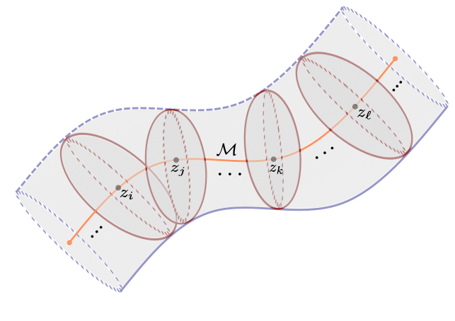
  Figure 3: The covering of tubular region $\mathcal{M}(q)$, where each ellipsoid represents the region $\{x:\tilde{\eta}_{i}(x)>0\}$.

  $\bullet$ Implementing the Oracle Approximator by Transformers 
  Since each $\tilde{\eta}_{i}(x)$ in (22) is composition of basic arithmetic operations, we can represent it without error by using transformer network. The first result in this subsection establishes the result for representing each $\tilde{\eta}_{i}(x)$.

  Proposition 1

  Suppose the Assumption 1 holds. Let $\{\tilde{\eta}_{i}(x)\}_{i=1}^{K}$ be defined as (22). Then for each fixed $i$, there exists a transformer network ${\rm T}(\theta;\cdot)\in\mathcal{T}(L_{T},m_{T},d_{embed},\ell,L_{\rm FFN},w_{\rm FFN},R,\kappa)$ with parameters

  $$\text{ }L_{T}=O(d),\text{ }m_{T}=O(D),\text{ }d_{embed}=O(1),\text{ }\ell\geq O(D),$$

  $$\text{ }L_{\rm FFN}=O(1),\text{ }w_{\rm FFN}=O(1),\text{ }\kappa=O(D^{2}\delta^{-8})$$

  such that

  $${\rm T}(\theta;x)=\tilde{\eta}_{i}(x)$$ (25)

  for any $x\in[0,1]^{D}$. The notation $O(\cdot)$ in $m_{T},\ell,\kappa$ hides the terms which are dependent on $d,q,\tau_{\mathcal{M}}$, while $O(\cdot)$ in others hides the terms dependent on $q,\tau_{\mathcal{M}}$.

The proof of Proposition 1 is deferred to Appendix C. The main theme of the proof is that, from (22), it is easy to see that $\tilde{\eta}_{i}(x)$ is built from a sequence basic arithmetic operations such as constant addition, constant multiplication, squaring, etc,. Each of these operations is implemented in Table 1. By chaining these operations sequentially, we get the corresponding ${\rm T}(\theta;\cdot)$ to represent $\tilde{\eta}_{i}(\cdot)$.

Once each $\tilde{\eta}_{i}$ is represented by ${\rm T}(\theta;\cdot)$, we can apply Lemma 7 to construct another transformer network which implements $\eta_{i}(x)=\tilde{\eta}_{i}(x)/\|\tilde{\eta}(x)\|_{1}$, $i=1,\cdots,K$, and $\eta(x)=(\eta_{1}(x),\cdots,\eta_{K}(x))$ within some tolerance. Then take the linear combination of those $\eta_{i}(x)$ to approximate $\hat{f}$. Note that we need to satisfies $\delta\in(0,\tau_{\mathcal{M}}/2)$ in order to have the cardinality $K=O(\delta^{-d})$ (see Lemma 6.1 in [Cloninger and Klock, 2021]), where $O(\cdot)$ hides the terms dependent in $d$ and the volume of manifold $\text{Vol}(\mathcal{M})$.

The approximation result for $\eta_{i}(x)$ is presented in Proposition 2 and its proof is deferred to Appendix C.

Proposition 2

Suppose Assumption 1 holds. Let $Z=\{z_{1},\cdots,z_{K}\}$ be a maximal separated $\delta$-net of $\mathcal{M}$ with respect to $d_{\mathcal{\mathcal{M}}}$ such that $\delta\in(0,\tau_{\mathcal{M}}/2)$, and define $\eta$ according to (23). Then for any $\epsilon\in(0,1)$, there exists ${\rm T}(\theta;\cdot)=({\rm T}^{1}(\theta;\cdot),\cdots,{\rm T}^{K}(\theta;\cdot))$ with each ${\rm T}^{i}(\theta;\cdot)\in\mathcal{T}(L_{T},m_{T},d_{embed},\ell,L_{\rm FFN},w_{\rm FFN},R,\kappa)$ such that for any $x\in\mathcal{M}(q)$,

$$|{\rm T}^{i}(\theta;x)-\eta_{i}(x)|\leq\epsilon\eta_{i}(x).$$ (26)

Consequently, $T(\theta;\cdot)$ satisfies

$$\textstyle\sup_{x\in\mathcal{M}(q)}\|{\rm T}(\theta;x)-\eta(x)\|_{1}\leq\epsilon.$$ (27)

The network ${\rm T}(\theta;\cdot)$ has parameters

$$L_{T}=O(d+\ln(\ln(\epsilon^{-1}))),\text{ }m_{T}=O(D\delta^{-d}),$$

$$d_{embed}=O(1),\text{ }\ell\geq O(D\delta^{-d}),\text{ }L_{\rm FFN}=O(1),$$

$$w_{\rm FFN}=O(1),\text{ }\kappa=O(D^{2}\delta^{-2d-8})$$

where $O(\cdot)$ in $m_{T}$, $\ell$, $\kappa$ hides the terms which are dependent on $d,q,\tau_{\mathcal{M}},\text{Vol}(\mathcal{M})$, while $O(\cdot)$ in others hides the terms which are dependent on $q,\tau_{\mathcal{M}},\text{Vol}(\mathcal{M})$.

With Proposition 2, we can approximates the $\hat{f}$ in (21) easily by scaling down the tolerance with the supremum norm of $g$. Let ${\rm T}_{1}(\theta;\cdot):=({\rm T}_{1}^{1}(\theta;\cdot),\cdots,{\rm T}_{1}^{K}(\theta;\cdot))$ where each ${\rm T}_{1}^{i}$ approximates $\eta_{i}$ such that

$$\textstyle\sup_{x\in\mathcal{M}(q)}\|{\rm T}_{1}(\theta;x)-\eta(x)\|_{1}\leq{\epsilon}/{\|g\|_{L^{\infty}(\mathcal{M})}}.$$

Then by Lemma 3 with constant $c=(g(z_{1}),\cdots g(z_{K}))$ and Lemma 1, we can construct ${\rm B}_{1},{\rm B}_{2}\in\mathcal{B}(K,3,d_{embed})$ such that ${\rm T}_{2}:={\rm B}_{2}\circ{\rm B}_{1}$ implements the approximation of $\sum_{i=1}^{K}g(z_{i}){\rm T}_{1}^{i}(\theta;x)$, where ${\rm T}_{2}$ has $L_{{\rm T}_{2}}=O(1)$ and $m_{{\rm T}_{2}}=K=O(\delta^{-d})$. Let ${\rm T}:={\rm T}_{2}\circ{\rm T}_{1}$, then for any $x\in\mathcal{M}(q)$, we have

$$\textstyle|{\rm T}(\theta;x)-\hat{f}(x)| =|\sum_{i=1}^{K}g(z_{i}){\rm T}_{1}^{i}(\theta;x)-\sum_{i=1}^{K}g(z_{i})\eta_{i}(x)|$$

$$\leq\|g\|_{L^{\infty}(\mathcal{M})}\|{\rm T}_{1}(\theta;x)-\eta(x)\|_{1}=\epsilon.$$

An illustration of the constructed transformer network architecture for approximating $\hat{f}$ is provided in Figure 2.

$\bullet$ Putting Error Bounds Together
For any partition of unity $\{\eta_{i}(x)\}_{i=1}^{K}$ subject to the covering $\{\pi^{-1}_{\mathcal{M}}(U_{i})\}_{i=1}^{K}$, we can write $f$ as $f(x)=\sum_{i=1}^{K}f(x)\eta_{i}(x)$. We consider the following piecewise constant approximation of $f$:

$$f(x)=\sum_{i=1}^{K}f(x)\eta_{i}(x)\approx\hat{f}(x):=\sum_{i=1}^{K}g(z_{i})\eta_{i}(x),$$ (28)

By the triangle inequality, for any $x\in\mathcal{M}(q)$,

$$|f(x)-T(\theta;x)|\leq|f(x)-\hat{f}(x)|+|\hat{f}(x)-T(\theta;x)|.$$

For the first term, we have

$$|f(x)-\hat{f}(x)| =\left|\sum_{i=1}^{K}g(\pi_{\mathcal{M}}(x))\eta_{i}(x)-\sum_{i=1}^{K}g(z_{i})\eta_{i}(x)\right|\leq\sum_{i=1}^{K}\left|g(\pi_{\mathcal{M}}(x))-g(z_{i})\right|\eta_{i}(x)$$

$$\leq L\sum_{i=1}^{K}d^{\alpha}_{\mathcal{M}}(\pi_{\mathcal{M}}(x),z_{i})\eta_{i}(x)\leq L\sum_{i=1}^{K}\left(\frac{72\delta}{(1-q)^{2}}\right)^{\alpha}\eta_{i}(x)=L\left(\frac{72\delta}{(1-q)^{2}}\right)^{\alpha}.$$

The last equality is due to partition of unity, and the inequality before the last equality is from Proposition 6.3 in [Cloninger and Klock, 2021].

For the second term, by Proposition 2 and its discussion, there exists a transformer network $T(\theta;\cdot)\in\mathcal{T}$ with parameters $L_{T}=O(d+\ln(\ln(\delta^{-\alpha})))$, $m_{T}=O(D\delta^{-d})$, $d_{embed}=O(1)$, $\ell=O(D\delta^{-d})$, $L_{FFN}=O(1)$, $w_{FFN}=O(1)$, $\kappa=O(D^{2}\delta^{-2d-8})$, such that

$$\|T(\theta;\cdot)-\hat{f}\|_{\mathcal{L}^{\infty}(\mathcal{M}(q))}\leq\delta^{\alpha}.$$ (29)

Thus

$$|T(\theta;x)-f(x)|\leq L\left(\frac{72\delta}{(1-q)^{2}}\right)^{\alpha}+\delta^{\alpha}=\left(1+L\left(\frac{72}{(1-q)^{2}}\right)^{\alpha}\right)\delta^{\alpha}.$$

By choosing $\delta$ such that $\left(1+L\left(\frac{72}{(1-q)^{2}}\right)^{\alpha}\right)\delta^{\alpha}=\epsilon$, we get $\delta=O(\epsilon^{1/\alpha})$ and

$$|T(\theta;x)-f(x)|\leq\epsilon.$$

Such a transformer network $T(\theta;\cdot)\in\mathcal{T}$ has parameters $L_{T}=O(d+\ln(\ln(\epsilon^{-1})))$, $m_{T}=O(D\epsilon^{-\frac{d}{\alpha}})$, $d_{embed}=O(1)$, $\ell\geq O(D\epsilon^{-\frac{d}{\alpha}})$, $L_{FFN}=O(1)$, $w_{FFN}=O(1)$, $\kappa=O(D^{2}\epsilon^{-\frac{2d+8}{\alpha}})$.

$\Box$

4.3 Proof of Theorem 2

Theorem 2 is proved via a bias-variance decomposition. The bias reflects the approximation error of $f$ by a constructed transformer network, while the variance captures the stochastic error in estimating the parameters of the constructed transformer network. For the bias term, we can bound it by using the approximation error bound in Theorem 1. The variance term can be bounded using the covering number of transformers (see Lemma 10).

• Proof. [Proof of Theorem 2]

  By adding and subtracting the twice of the bias term, we can rewrite the squared generalization error as

  $$\mathbb{E}\|\hat{T}_{n}-f\|^{2}_{L^{2}(P)} =\mathbb{E}\int_{\mathcal{M}(q)}(\hat{T}_{n}(x)-f(x))^{2}dP$$

  $$=\mathbb{E}\left[\frac{2}{n}\sum_{i=1}^{n}(\hat{T}_{n}(x_{i})-f(x_{i}))^{2}\right]+\mathbb{E}\int_{\mathcal{M}(q)}(\hat{T}_{n}(x)-f(x))^{2}dP-\mathbb{E}\left[\frac{2}{n}\sum_{i=1}^{n}(\hat{T}_{n}(x_{i})-f(x_{i}))^{2}\right].$$

  By Jensen’s inequality, the bias term satisfies

  $$\mathbb{E}\left[\frac{1}{n}\sum_{i=1}^{n}(\hat{T}_{n}(x_{i})-f(x_{i}))^{2}\right] =\mathbb{E}\inf_{T\in\mathcal{T}}\left[\frac{1}{n}\sum_{i=1}^{n}(T(x_{i})-f(x_{i}))^{2}\right]\leq\inf_{T\in\mathcal{T}}\mathbb{E}\left[\frac{1}{n}\sum_{i=1}^{n}(T(x_{i})-f(x_{i}))^{2}\right]$$

  $$=\inf_{T\in\mathcal{T}}\int_{\mathcal{M}(q)}(T(x)-f(x))^{2}dP\leq\inf_{T\in\mathcal{T}}\int_{\mathcal{M}(q)}\|T-f\|^{2}_{L^{\infty}(\mathcal{M}(q))}dP$$

  $$=\inf_{T\in\mathcal{T}}\|T-f\|^{2}_{L^{\infty}(\mathcal{M}(q))}\leq O(\epsilon^{2}).$$

  By Lemma 6 in [Chen et al., 2022], the variance term has the bound

  $$\mathbb{E}\int_{\mathcal{M}(q)}(\hat{T}_{n}(x)-f(x))^{2}dP -\mathbb{E}\left[\frac{2}{n}\sum_{i=1}^{n}(\hat{T}_{n}(x_{i})-f(x_{i}))^{2}\right]$$

  $$\leq\inf_{\delta>0}\left[\frac{104R^{2}}{3n}\ln\mathcal{N}\left(\frac{\delta}{4R},\mathcal{T},\|\cdot\|_{\infty}\right)+\left(4+\frac{1}{2R}\right)\delta\right]$$

  $$\leq\left[\frac{104R^{2}}{3n}\ln\mathcal{N}\left(\frac{1}{4nR},\mathcal{T},\|\cdot\|_{\infty}\right)+\left(4+\frac{1}{2R}\right)\frac{1}{n}\right]$$

  where $\mathcal{N}\left(\frac{\delta}{4R},\mathcal{T},\|\cdot\|_{\infty}\right)$ is the covering number (defined in Definition 7) of transformer network class $\mathcal{T}$ with $L^{\infty}$ norm.

By Lemma 10, we get

$$\ln\mathcal{N}\left(\frac{1}{4nR},\mathcal{T},\|\cdot\|_{\infty}\right) \leq\ln\left(2^{L_{T}+3}nRL_{\text{FFN}}d_{embed}^{18L_{T}^{2}}w_{\text{FFN}}^{18L_{T}^{2}L_{\text{FFN}}}\kappa^{6L_{T}^{2}L_{\text{FFN}}}m_{T}^{L_{T}^{2}}\ell^{L_{T}^{2}}\right)^{4d^{2}_{embed}w^{2}_{\text{FFN}}D(m_{T}+L_{\text{FFN}})L_{T}}$$

$$\leq(4d^{2}_{embed}w^{2}_{\text{FFN}}D(m_{T}+L_{\text{FFN}})L_{T})(18L^{2}_{T}L_{\text{FFN}}\ln(2nRL_{\text{FFN}}d_{embed}w_{\text{FFN}}\kappa m_{T}\ell))$$

$$\leq 72\ln(2nRL_{\text{FFN}}d_{embed}w_{\text{FFN}}\kappa m_{T}\ell)d^{2}_{embed}w^{2}_{\text{FFN}}Dm_{T}L^{3}_{T}L^{2}_{\text{FFN}}.$$

For target accuracy $\epsilon$, we know from Theorem 1 that $L_{T}=O(d+\ln(\ln(\epsilon^{-1})))$, $m_{T}=O(D\epsilon^{-\frac{d}{\alpha}})$, $d_{embed}=O(1)$, $\ell=O(D\epsilon^{-\frac{d}{\alpha}})$, $L_{\rm FFN}=O(1)$, $w_{\rm FFN}=O(1)$, $\kappa=O(D^{2}\epsilon^{-\frac{2d+8}{\alpha}})$, where $O(\cdot)$ hides the constant terms in $d,q,\tau_{\mathcal{M}},\text{Vol}(\mathcal{M})$. This simplifies the above to

$$\ln\mathcal{N}\left(\frac{1}{4nR},\mathcal{T},\|\cdot\|_{\infty}\right)\leq\tilde{O}(D^{2}d^{3}\epsilon^{-\frac{d}{\alpha}})$$

where $\tilde{O}(\cdot)$ hides the logarithmic terms in $D,d,q,n,\epsilon,\alpha,L,R,\tau_{\mathcal{M}}$,$\text{Vol}(\mathcal{M})$ and constant terms in $d$ and $\text{Vol}(\mathcal{M})$. Thus, the variance term is bounded by

$$\mathbb{E}\int_{\mathcal{M}(q)}(\hat{T}_{n}(x)-f(x))^{2}dP-\mathbb{E}\left[\frac{2}{n}\sum_{i=1}^{n}(\hat{T}_{n}(x_{i})-f(x_{i}))^{2}\right]\leq\tilde{O}\left(\frac{D^{2}d^{3}\epsilon^{-\frac{d}{\alpha}}}{n}\right).$$

Putting the bias and variance together, we get

$$\mathbb{E}\|\hat{T}_{n}-f\|^{2}_{L^{2}(P)}\leq\tilde{O}\left(\epsilon^{2}+\frac{D^{2}d^{3}\epsilon^{-\frac{d}{\alpha}}}{n}\right).$$ (30)

By balancing the bias and variance, i.e., setting $\epsilon^{2}=\frac{\epsilon^{-\frac{d}{\alpha}}}{n}$, we get $\epsilon=n^{-\frac{\alpha}{2\alpha+d}}$. This yields

$$\mathbb{E}\|\hat{T}_{n}-f\|^{2}_{L^{2}(P)}\leq\tilde{O}\left(D^{2}d^{3}n^{-\frac{2\alpha}{2\alpha+d}}\right)$$ (31)

as desired.

$\Box$

Remark 1

It is worth pointing out that the factor of two included in the proof is intended to enhance the rate of convergence of the statistical error.

5 Experiments

Our theoretical results show that transformers can recover low-dimensional structures even when training data itself may not exactly lie on a low-dimensional manifold. To validate this findings, we conduct a series of experiments measuring the intrinsic dimension of common computer vision datasets with various levels of isotropic Gaussian noise. We then embed noisy image data using a pre-trained vision transformer (ViT) [Dosovitskiy et al., 2021] and measure the intrinsic dimension of the resulting embeddings.
Setup. We measure the validation split of Imagenet-1k [Deng et al., 2009]. We first pre-process images by rescaling to $D=224\times 244$ dimensions and normalizing pixel values inside of the $[-1,1]^{D}$ cube. We use the pre-trained google/vit-base-patch16-224 model to produce image embeddings of size $196\times 768$. To measure intrinsic dimension we use the MLE estimator [Levina and Bickel, 2004] with $K=30$ neighbors with batch size $4096$ averaged over 50,000 images. We flatten all images beforehand.

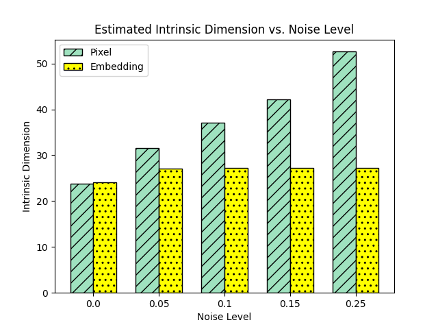
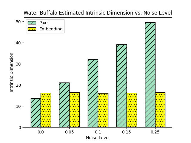
Figure 4: Left subplot: Estimated intrinsic dimension (ID) of pixel and embedded image representations with various amounts of isotropic Gaussian noise. Noise added on pixels quickly distorts low-dimensional structures. Embedding with the pre-trained model demonstrates a denoising effect, recovering the original ID at all noise levels. Right subplot: Estimated intrinsic dimension of water buffalo images and embeddings across various noise levels.

Results. Figure 4 shows that, with no noise, the intrinsic dimensions of this dataset in both pixel and embedding space are measured to be  25. As isotropic Gaussian noise with increasing variance is added, the intrinsic dimension of pixel data quickly increases. However, the intrinsic dimension of the embedded noisy pixel data remains constant, demonstrating the strong denoising effect of the vision transformer.

Figure 4 also measures the intrinsic dimension of the water buffalo subset of Imagenet (class 346) across various noise levels. The estimated image dimension is around 15 while the estimated embedding dimension is around 18. However, adding isotropic Gaussian noise quickly increases the intrinsic dimension of images while having a negligible effect on the intrinsic dimension of embeddings.

6 Conclusion and Discussion

This paper establishes approximation and generalization bounds of transformers for functions which depend on the projection of the input onto a low-dimensional manifold. This regression model is interesting in machine learning applications where the input data contain noise or the function has low complexity depending on a low-dimensional task manifold. Our theory justifies the capability of transformers in handling noisy data and adapting to low-dimensional structures in the prediction tasks.
This work considers Hölder functions with Hölder index $\alpha\in(0,1]$. How to estimate this Hölder index is a practically interesting problem. How to extend the theory to more regular functions with $\alpha>1$ is a theoretically interesting problem. More broadly, our work improves fundamental understanding of transformers and improves our ability to theoretically and safely predict future capabilities.

Appendix A Table of Notations

Our notations are summarized in Table 2.

Table 2: Table of notations

Symbol	Interpretation
$\mathcal{M}$	A manifold
Vol$(\mathcal{M})$	Volume of the manifold $\mathcal{M}$
Med($\mathcal{M}$)	medial axis of a manifold $\mathcal{M}$
$\tau_{\mathcal{}}(v)$	local reach at of $\mathcal{M}$ at $v$
$\tau_{\mathcal{M}}$	local reach of $\mathcal{M}$
$\pi_{\mathcal{M}}(x)$	projection of $x\in\mathcal{M}(q)$ onto $\mathcal{M}$
$P(v)$	$D\times d$ matrix consists of orthonormal basis of the tangent space of $\mathcal{M}$ at $v$.
$d_{\mathcal{M}}(x,x^{\prime})$	geodesic distance between $x$ and $x^{\prime}$
$d_{\mathcal{M}(q)}(v,v^{\prime})$	tubular geodesic distance between $v$ and $v^{\prime}$
$\{z_{1},\cdots,z_{K}\}$	a maximal separated $\delta$-net of $\mathcal{M}$ with respect to $d_{\mathcal{\mathcal{M}}}$
$x=(x^{1},\cdots,x^{D})$	input variable
$H$	embedding matrix
$d_{embed}$	embedding dimension
${\rm T}$	a transformer network
${\rm B}$	a transformer block
$L_{T}$	number of transformer blocks in ${\rm T}$
$m_{T}$	maximum number of attention heads in each block of ${\rm T}$
$\ell$	number of hidden tokens
$\mathcal{I}_{j}$	interaction term $(\cos(\frac{j\pi}{2\ell}),\sin(\frac{j\pi}{2\ell}))^{\top}$
$H_{i,j}$	the $(i,j)$-th entry of $H$
$H_{J,:}$	submatrix of $H$ with rows with row index in $J$ and all the columns
$H_{:,J}$	submatrix of $H$ with all the rows and columns with column index in $J$
$x\odot x$	componentwise product, i.e., $x\odot x=((x^{1})^{2},\cdots,(x^{D})^{2})$
$x^{\circ r}$	componentwise $r$-th power, i.e., $x^{\circ r}=((x^{1})^{r},\cdots,(x^{D})^{r})$
$\|x\|_{1}$	$\ell^{1}$ norm of a vector $x$
$\|x\|_{\infty}$	maximum norm of a vector $x$
$\|M\|_{\infty,\infty}$	maximum norm of a matrix $M$

Appendix B Implementing Basic Arithmetic Operations by Transformers

B.1 Interaction Lemma and Gating Lemma

We first present two lemmas which will be useful when building the arithmetic operations. The first lemma is called Interaction Lemma.

Lemma 8 (Interaction Lemma)

Let $H=[h_{t}]_{1\leq t\leq\ell}\in\mathbb{R}^{d_{embed}\times\ell}$ be an embedding matrix such that $h_{t}^{(d_{embed}-2):(d_{embed}-1)}=\mathcal{I}_{t}$ and $h^{d_{embed}}_{t}=1$. Fix $1\leq t_{1},t_{2}\leq\ell,1\leq i\leq d_{embed}$, and $\ell\in\mathbb{N}$. Suppose $d_{embed}\geq 5$ and $\|H\|_{\infty,\infty}<M$ for some $M>0$, and the data kernels $Q^{data}$ (first two rows in the query matrix $Q$) and $K^{data}$ (first two rows in the key matrix $K$) satisfy $\max\{\|Q^{data}\|_{\infty,\infty},\|K^{data}\|_{\infty,\infty}\}\leq\mu$. Then we can construct an attention head $A$ with $\|\theta_{A}\|_{\infty}=O(d_{embed}^{4}\mu^{2}\ell^{2}M^{2})$ such that

$$A(h_{t})=\begin{cases}\sigma(\langle Q^{data}h_{t},K^{data}h_{t_{2}}\rangle)e_{i}&\text{if}\text{ }t=t_{1},\\ 0&\text{otherwise}.\\ \end{cases}$$

• Proof. We refer its proof to Lemma 3 in [Havrilla and Liao, 2024]. $\Box$

Remark 2

The significance of the Interaction Lemma is that we can find an attention head such that one token interacts with exactly another token in the embedding matrix. This property facilitates the flexible implementation of fundamental arithmetic operations, such as addition, multiplication, squaring, etc., while also supporting efficient parallelization.

The next lemma shows the way to zero out the contiguous tokens in the embedding matrix while keep other tokens unchanged via a feed-forward network.

Lemma 9 (Gating Lemma)

Let $d_{embed}\geq 5$ and $H=[h_{t}]_{1\leq t\leq\ell}\in\mathbb{R}^{d_{embed}\times\ell}$, be an embedding matrix such that $h_{t}^{(d_{embed}-2):(d_{embed}-1)}=\mathcal{I}_{t}$ and $h^{d_{embed}}_{t}=1$. Then there exists a two-layer feed-forward network (FFN) such that

$$\text{\rm FFN}(h_{t})=\begin{cases}h_{t}&\text{if}\text{ }t\in\{1,\cdots,k\}\\ \begin{bmatrix}\mathbf{0}\\ \mathcal{I}_{t}^{1}\\ \mathcal{I}_{t}^{2}\\ 1\end{bmatrix}&\text{otherwise}\text{ }\\ \end{cases}$$

Additionally, we have $\|\theta_{\rm FFN}\|_{\infty}\leq O(\ell\|H\|_{\infty})$.

• Proof. We refer its proof to Lemma 4 in [Havrilla and Liao, 2024]. $\Box$

B.2 Proof of Basic Arithmetic Operations

B.2.1 Proof of Lemma 1

• Proof. [Proof of Lemma 1] Let us define each attention head $A_{i}$, $1\leq i\leq D$, with the data kernel in the form

  $$Q_{i}^{data}=\begin{bmatrix}0&0&0&0&1\\ 0&0&0&0&1\end{bmatrix}\quad K_{i}^{data}=\begin{bmatrix}1&0&0&0&0\\ 0&0&0&0&M\end{bmatrix}.$$

  Let $h_{i}$ denote the $i$-th column of $H$, $1\leq i\leq\ell$. By Interaction Lemma 8, we can construct $A_{i}$, $1\leq i\leq D$, such that $h_{D+1}$ interacts with $h_{i}$ only, i.e.,

  $$A_{i}(h_{D+1})=\sigma(\langle Q_{i}^{data}h_{D+1},K_{i}^{data}h_{i}\rangle)e_{1}=\sigma(x^{i}+M)e_{1}=(x^{i}+M)e_{1},$$

  and $A_{i}(h_{t})=0$ when $t\neq D+1$. Then the residual multi-head attention yields

  $$\text{MHA}(H)+H=\begin{bmatrix}x^{1}&\cdots&x^{D}&x^{1}+\cdots+x^{D}+DM&\mathbf{0}\\ 0&\cdots&\cdots&\cdots&0\\ \mathcal{I}_{1}&\cdots&\cdots&\cdots&\mathcal{I}_{\ell}\\ 1&\cdots&\cdots&\cdots&1\end{bmatrix}.$$

  Then we apply the Gating Lemma 9 to have a $\mathcal{FFN}(3)$ to subtract off the constant $DM$ in the $D+1$-th column. Thus

  $$B(H)=\begin{bmatrix}x^{1}&\cdots&x^{D}&x^{1}+\cdots+x^{D}&\mathbf{0}\\ 0&\cdots&\cdots&\cdots&0\\ \mathcal{I}_{1}&\cdots&\cdots&\cdots&\mathcal{I}_{\ell}\\ 1&\cdots&\cdots&\cdots&1\end{bmatrix}$$

  as desired. The weights $\|\theta_{B}\|_{\infty}\leq O(\ell^{2}M^{2}\|H\|^{2}_{\infty,\infty})$ follows from Interaction Lemma 8. $\Box$

Remark 3

By reexamining the proof, it is easy to see that the summation term $x^{1}+\cdots+x^{D}$ can be put in any column of the first row, not necessarily the $D+1$-th column. This provides a lot of flexibility when parallelizing different basic operations in one transformer block.

B.2.2 Proof of Lemma 2

• Proof.[Proof of Lemma 2] Let us define the each attention head $A_{i}$, $1\leq i\leq D$, with the data kernel in the form

  $$Q_{i}^{data}=\begin{bmatrix}0&0&0&0&0\\ 0&0&0&0&1\end{bmatrix}\quad K_{i}^{data}=\begin{bmatrix}0&0&0&0&0\\ 1&0&0&0&c^{i}+M\end{bmatrix}.$$

  By Interaction Lemma 8, we can construct $A_{i}$ such that $h_{D+i}$ interacts with $h_{i}$ only, i.e.,

  $$A_{i}(h_{D+i})=\sigma(\langle Q_{i}^{data}h_{D+i},K_{i}^{data}h_{i}\rangle)e_{1}=\sigma(x^{i}+c^{i}+M)e_{1}=(x^{i}+c^{i}+M)e_{1},$$

  and $A_{i}(h_{t})=0$ when $t\neq D+i$. Then the residual multi-head attention yields

  $$\text{MHA}(H)+H=\begin{bmatrix}x^{1}&\cdots&x^{D}&x^{1}+c^{1}+M&\cdots&x^{D}+c^{D}+M&\mathbf{0}\\ 0&\cdots&\cdots&\cdots&\cdots&\cdots&0\\ \mathcal{I}_{1}&\cdots&\cdots&\cdots&\cdots&\cdots&\mathcal{I}_{\ell}\\ 1&\cdots&\cdots&\cdots&\cdots&\cdots&1\end{bmatrix}.$$

  Then we apply the Gating Lemma 9 to have a $\mathcal{FFN}(3)$ to subtract off the constant $M$ only from columns $D+1$ to $2D$. Therefore, we have

  $$B(H)=\begin{bmatrix}x^{1}&\cdots&x^{D}&x^{1}+c^{1}&\cdots&x^{D}+c^{D}&\mathbf{0}\\ 0&\cdots&\cdots&\cdots&\cdots&\cdots&0\\ \mathcal{I}_{1}&\cdots&\cdots&\cdots&\cdots&\cdots&\mathcal{I}_{\ell}\\ 1&\cdots&\cdots&\cdots&\cdots&\cdots&1\end{bmatrix}$$

  as desired. The weights $\|\theta_{B}\|_{\infty}\leq O(\ell^{2}M^{2}\|H\|^{2}_{\infty,\infty})$ follows from Interaction Lemma 8. $\Box$

B.2.3 Proof of Lemma 3

• Proof. [Proof of Lemma 3] Let us define the each attention head $A_{i}$, $1\leq i\leq D$, with the data kernel in the form

  $$Q_{i}^{data}=\begin{bmatrix}0&0&0&0&c^{i}\\ 0&0&0&0&1\end{bmatrix}\quad K_{i}^{data}=\begin{bmatrix}1&0&0&0&0\\ 0&0&0&0&M\end{bmatrix}.$$

  Then by Interaction Lemma 8, we can construct $A_{i}$ such that $h_{D+i}$ interacts with $h_{i}$ only, i.e.,

  $$A_{i}(h_{D+i})=\sigma(\langle Q_{i}^{data}h_{D+i},K_{i}^{data}h_{i}\rangle)e_{1}=\sigma(c^{i}x^{i}+M)e_{1}=(c^{i}x^{i}+M)e_{1},$$

  and $A_{i}(h_{t})=0$ when $t\neq D+i$. Then the residual multi-head attention yields

  $$\text{MHA}(H)+H=\begin{bmatrix}x^{1}&\cdots&x^{D}&c^{1}x^{1}+M&\cdots&c^{D}x^{D}+M&\mathbf{0}\\ 0&\cdots&\cdots&\cdots&\cdots&\cdots&0\\ \mathcal{I}_{1}&\cdots&\cdots&\cdots&\cdots&\cdots&\mathcal{I}_{\ell}\\ 1&\cdots&\cdots&\cdots&\cdots&\cdots&1\end{bmatrix}.$$

  Then we apply the Gating Lemma 9 to have a $\mathcal{FFN}(3)$ to subtract off the constant $M$ only from columns $D+1$ to $2D$. Thus

  $$B(H)=\begin{bmatrix}x^{1}&\cdots&x^{D}&c^{1}x^{1}&\cdots&c^{D}x^{D}&\mathbf{0}\\ 0&\cdots&\cdots&\cdots&\cdots&\cdots&0\\ \mathcal{I}_{1}&\cdots&\cdots&\cdots&\cdots&\cdots&\mathcal{I}_{\ell}\\ 1&\cdots&\cdots&\cdots&\cdots&\cdots&1\end{bmatrix}.$$

  as desired. The weights $\|\theta_{B}\|_{\infty}\leq O(\ell^{2}M^{2}\|H\|^{2}_{\infty,\infty})$ follows from Interaction Lemma 8. $\Box$

B.2.4 Proof of Lemma 4

• Proof. [Proof of Lemma 4] First, applying Lemma 3 with multiplication constant $c=(1,\cdots,1)$, we can construct the transformer block $B_{1}\in\mathcal{B}(D,3,d_{embed})$ so that it copies the first $D$ elements in the first row from columns $1,\cdots,D$ to columns $D+1,\cdots,2D$, i.e.,

  $$H_{1}:=B_{1}(H)=\begin{bmatrix}x^{1}&\cdots&x^{D}&x^{1}&\cdots&x^{D}&\mathbf{0}\\ 0&\cdots&\cdots&\cdots&\cdots&\cdots&0\\ \mathcal{I}_{1}&\cdots&\cdots&\cdots&\cdots&\cdots&\mathcal{I}_{\ell}\\ 1&\cdots&\cdots&\cdots&\cdots&\cdots&1\end{bmatrix}.$$

  For $B_{2}$, let us define each attention head $A_{i}$, $1\leq i\leq D$, with the data kernel in the form

  $$Q_{i}^{data}=\begin{bmatrix}1&0&0&0&0\\ 0&0&0&0&0\end{bmatrix}\quad K_{i}^{data}=\begin{bmatrix}1&0&0&0&0\\ 0&0&0&0&0\end{bmatrix}.$$

  Let $h_{1,i}$ denote the $i$-th column of $H_{1}$, $1\leq i\leq\ell$. By Interaction Lemma 8, we can construct $A_{i}$, $1\leq i\leq D$, such that $h_{1,D+i}$ interacts with $h_{1,i}$ only, i.e.,

  $$A_{i}(h_{1,D+i})=\sigma(\langle Q_{i}^{data}h_{1,D+i},K_{i}^{data}h_{1,i}\rangle)e_{1}=\sigma((x^{i})^{2})e_{1}=(x^{i})^{2}e_{1},$$

  and $A_{i}(h_{1,t})=0$ when $t\neq D+i$. Then the residual multi-head attention yields

  $$\text{MHA}(H_{1})+H_{1}=\begin{bmatrix}x^{1}&\cdots&x^{D}&(x^{1})^{2}+x^{1}&\cdots&(x^{D})^{2}+x^{D}&\mathbf{0}\\ 0&\cdots&\cdots&\cdots&\cdots&\cdots&0\\ \mathcal{I}_{1}&\cdots&\cdots&\cdots&\cdots&\cdots&\mathcal{I}_{\ell}\\ 1&\cdots&\cdots&\cdots&\cdots&\cdots&1\end{bmatrix}.$$

  Let $H_{2}:=B_{2}(H_{1})=\text{MHA}(H_{1})+H_{1}$, and we use $h_{2,i}$ to denote the $i$-th column of $H_{2}$, $1\leq i\leq\ell$. Now again by Lemma 3 with multiplication constant $c=(-1,\cdots,-1)$, we can construct $B_{3}\in\mathcal{B}(D,3,d_{embed})$ with each attention head $\tilde{A}_{i}$, $1\leq i\leq D$, such that $h_{2,D+i}$ interacts with $h_{2,i}$ only. Let the data kernel of each $\tilde{A}_{i}$ in the form

  $$Q_{i}^{data}=\begin{bmatrix}0&0&0&0&-1\\ 0&0&0&0&1\end{bmatrix}\quad K_{i}^{data}=\begin{bmatrix}1&0&0&0&0\\ 0&0&0&0&M\end{bmatrix}.$$

  By Interaction Lemma 8, we have

  $$\tilde{A}_{i}(h_{2,D+i})=\sigma(\langle Q_{i}^{data}h_{2,D+i},K_{i}^{data}h_{2,i}\rangle)e_{1}=\sigma(-x^{i}+M)e_{1}=(-x^{i}+M)e_{1},$$

  and $\tilde{A}_{i}(h_{2,t})=0$ when $t\neq D+i$. Thus, the residual multi-head attention yields

  $$\text{MHA}(H_{2})+H_{2}=\begin{bmatrix}x^{1}&\cdots&x^{D}&(x^{1})^{2}+M&\cdots&(x^{D})^{2}+M&\mathbf{0}\\ 0&\cdots&\cdots&\cdots&\cdots&\cdots&0\\ \mathcal{I}_{1}&\cdots&\cdots&\cdots&\cdots&\cdots&\mathcal{I}_{\ell}\\ 1&\cdots&\cdots&\cdots&\cdots&\cdots&1\end{bmatrix}.$$

  Then we apply the Gating Lemma 9 to have a $\mathcal{FFN}(3)$ to subtract off the constant $M$ only from columns $D+1$ to $2D$. Therefore, we have

  $$B_{3}\circ B_{2}\circ B_{1}(H)=B_{3}(H_{2})=\begin{bmatrix}x^{1}&\cdots&x^{D}&(x^{1})^{2}&\cdots&(x^{D})^{2}&\mathbf{0}\\ 0&\cdots&\cdots&\cdots&\cdots&\cdots&0\\ \mathcal{I}_{1}&\cdots&\cdots&\cdots&\cdots&\cdots&\mathcal{I}_{\ell}\\ 1&\cdots&\cdots&\cdots&\cdots&\cdots&1\end{bmatrix}$$

  as desired. The weights $\|\theta_{B}\|_{\infty}\leq O(\ell^{2}M^{2}\|H\|^{2}_{\infty,\infty})$ follows from Interaction Lemma 8. $\Box$

B.2.5 Proof of Lemma 5

• Proof. [Proof of Lemma 5] First, applying Lemma 3 with multiplication constant $c=(1,\cdots,1)$, we can construct the transformer block $B_{1}\in\mathcal{B}(D,3,d_{embed})$ so that it copies the first $D$ elements in the first row from columns $1,\cdots,D$ to columns $2D+1,\cdots,3D$, i.e.,

  $$H_{1}:=B_{1}(H)=\begin{bmatrix}x^{1}&\cdots&x^{D}&y^{1}&\cdots&y^{D}&x^{1}&\cdots&x^{D}&\mathbf{0}\\ 0&\cdots&\cdots&\cdots&\cdots&\cdots&\cdots&\cdots&\cdots&0\\ \mathcal{I}_{1}&\cdots&\cdots&\cdots&\cdots&\cdots&\cdots&\cdots&\cdots&\mathcal{I}_{\ell}\\ 1&\cdots&\cdots&\cdots&\cdots&\cdots&\cdots&\cdots&\cdots&1\end{bmatrix}.$$

  For $B_{2}$, let us define the each attention head $A_{i}$, $1\leq i\leq D$, with the data kernel in the form

  $$Q_{i}^{data}=\begin{bmatrix}1&0&0&0&0\\ 0&0&0&0&1\end{bmatrix}\quad K_{i}^{data}=\begin{bmatrix}1&0&0&0&0\\ 0&0&0&0&M\end{bmatrix}.$$ (32)

  By Interaction Lemma 8, we can construct $A_{i}$, $1\leq i\leq D$, such that $h_{1,2D+i}$ interacts with $h_{1,D+i}$ only, i.e.,

  $$A_{i}(h_{1,2D+i})=\sigma(\langle Q_{i}^{data}h_{1,2D+i},K_{i}^{data}h_{1,D+i}\rangle)e_{1}=\sigma(x^{i}y^{i}+M)e_{1}=(x^{i}y^{i}+M)e_{1},$$

  and $A_{i}(h_{1,t})=0$ when $t\neq 2D+i$. Then the residual multi-head attention yields

  $$\text{MAH}(H_{1})+H_{1}=\begin{bmatrix}x^{1}&\cdots&x^{D}&y^{1}&\cdots&y^{D}&x^{1}y^{1}+x^{1}+M&\cdots&x^{D}y^{D}+x^{D}+M&\mathbf{0}\\ 0&\cdots&\cdots&\cdots&\cdots&\cdots&\cdots&\cdots&\cdots&0\\ \mathcal{I}_{1}&\cdots&\cdots&\cdots&\cdots&\cdots&\cdots&\cdots&\cdots&\mathcal{I}_{\ell}\\ 1&\cdots&\cdots&\cdots&\cdots&\cdots&\cdots&\cdots&\cdots&1\end{bmatrix}.$$

  Then we apply the Gating Lemma 9 to have a $\mathcal{FFN}(3)$ to subtract off the constant $M$ only from columns $2D+1$ to $3D$. Thus, we have

  $$H_{2}:=B_{2}\circ B_{1}(H)=B_{2}(H_{1})=\begin{bmatrix}x^{1}&\cdots&x^{D}&y^{1}&\cdots&y^{D}&x^{1}y^{1}+x^{1}&\cdots&x^{D}y^{D}+x^{D}&\mathbf{0}\\ 0&\cdots&\cdots&\cdots&\cdots&\cdots&\cdots&\cdots&\cdots&0\\ \mathcal{I}_{1}&\cdots&\cdots&\cdots&\cdots&\cdots&\cdots&\cdots&\cdots&\mathcal{I}_{\ell}\\ 1&\cdots&\cdots&\cdots&\cdots&\cdots&\cdots&\cdots&\cdots&1\end{bmatrix}.$$

  Now again by Lemma 3 with multiplication constant $c=(-1,\cdots,-1)$, we can construct $B_{3}\in\mathcal{B}(D,3,d_{embed})$ with each attention head $\tilde{A}_{i}$, $1\leq i\leq D$, such that $h_{2,2D+i}$ interacts with $h_{2,i}$ only. Let the data kernel of each $\tilde{A}_{i}$ in the form

  $$Q_{i}^{data}=\begin{bmatrix}0&0&0&0&-1\\ 0&0&0&0&1\end{bmatrix}\quad K_{i}^{data}=\begin{bmatrix}1&0&0&0&0\\ 0&0&0&0&M\end{bmatrix}.$$

  By Interaction Lemma 8, we have

  $$\tilde{A}_{i}(h_{2,2D+i})=\sigma(\langle Q_{i}^{data}h_{2,2D+i},K_{i}^{data}h_{2,i}\rangle)e_{1}=\sigma(-x^{i}+M)e_{1}=(-x^{i}+M)e_{1},$$

  and $\tilde{A}_{i}(h_{2,t})=0$ when $t\neq 2D+i$. Thus, the residual multi-head attention yields

  $$\text{MHA}(H_{2})+H_{2}=\begin{bmatrix}x^{1}&\cdots&x^{D}&y^{1}&\cdots&y^{D}&x^{1}y^{1}+M&\cdots&x^{D}y^{D}+M&\mathbf{0}\\ 0&\cdots&\cdots&\cdots&\cdots&\cdots&\cdots&\cdots&\cdots&0\\ \mathcal{I}_{1}&\cdots&\cdots&\cdots&\cdots&\cdots&\cdots&\cdots&\cdots&\mathcal{I}_{\ell}\\ 1&\cdots&\cdots&\cdots&\cdots&\cdots&\cdots&\cdots&\cdots&1\end{bmatrix}$$

  Then we apply the Gating Lemma 9 to have a $\mathcal{FFN}(3)$ to subtract off the constant $M$ only from columns $2D+1$ to $3D$. Therefore, we have

  $$B_{3}\circ B_{2}\circ B_{1}(H)=B_{3}(H_{2})=\begin{bmatrix}x^{1}&\cdots&x^{D}&y^{1}&\cdots&y^{D}&x^{1}y^{1}&\cdots&x^{D}y^{D}&\mathbf{0}\\ 0&\cdots&\cdots&\cdots&\cdots&\cdots&\cdots&\cdots&\cdots&0\\ \mathcal{I}_{1}&\cdots&\cdots&\cdots&\cdots&\cdots&\cdots&\cdots&\cdots&\mathcal{I}_{\ell}\\ 1&\cdots&\cdots&\cdots&\cdots&\cdots&\cdots&\cdots&\cdots&1\end{bmatrix}$$

  as desired. The weights $\|\theta_{B}\|_{\infty}\leq O(\ell^{2}M^{2}\|H\|^{2}_{\infty,\infty})$ follows from Interaction Lemma 8. $\Box$

B.2.6 Proof of Lemma 6

• Proof. [Proof of Lemma 6] It suffices to show for the case $r=2^{s}$. Let us proceed by induction on $s$. First, suppose $B_{1},B_{2},B_{3}\in\mathcal{B}(D,3,d_{embed})$ implements the squaring operation as shown in Lemma 4, i.e.,

  $$H_{3}:=B_{3}\circ B_{2}\circ B_{1}(H)=\begin{bmatrix}x^{1}&\cdots&x^{D}&(x^{1})^{2}&\cdots&(x^{D})^{2}&\mathbf{0}\\ 0&\cdots&\cdots&\cdots&\cdots&\cdots&0\\ \mathcal{I}_{1}&\cdots&\cdots&\cdots&\cdots&\cdots&\mathcal{I}_{\ell}\\ 1&\cdots&\cdots&\cdots&\cdots&\cdots&1\end{bmatrix}.$$

  For the next three blocks $B_{4},B_{5},B_{6}$, we can apply Lemma 3 with $c=(1,\cdots,1)$ on $B_{4}\in\mathcal{B}(2D,3,d_{embed})$ to copy the nonzero elements in the first row from columns $1,\cdots,2D$ to columns $2D+1,\cdots,4D$. Apply Lemma 5 on $B_{5}\in\mathcal{B}(2D,3,d_{embed})$ such that $h_{4,2D+i}$ interacts only with $h_{4,D+i}$, and $h_{4,3D+i}$ interacts only with $h_{4,D+i}$, $1\leq i\leq D$. Then apply Lemma 3 with $c=(-1,\cdots,-1)$ on $B_{6}\in\mathcal{B}(2D,3,d_{embed})$ such that $h_{5,2D+i}$ interacts only with $h_{5,i}$ and $h_{5,3D+i}$ interacts only with $h_{5,D+i}$, $1\leq i\leq D$.

  Then we have

  $$H_{6}:=B_{6}\circ B_{5}\circ\cdots\circ B_{1}(H)=\begin{bmatrix}x^{1}&\cdots&x^{D}&\cdots&(x^{1})^{4}&\cdots&(x^{D})^{4}&\mathbf{0}\\ 0&\cdots&\cdots&\cdots&\cdots&\cdots&\cdots&0\\ \mathcal{I}_{1}&\cdots&\cdots&\cdots&\cdots&\cdots&\cdots&\mathcal{I}_{\ell}\\ 1&\cdots&\cdots&\cdots&\cdots&\cdots&\cdots&1\end{bmatrix}.$$

  Now suppose in the $(s-1)$-th step, we have

  $$H_{3s-3}:=B_{3s-3}\circ\cdots\circ B_{1}(H)=\begin{bmatrix}x^{1}&\cdots&x^{D}&\cdots&(x^{1})^{2^{s-1}}&\cdots&(x^{D})^{2^{s-1}}&\mathbf{0}\\ 0&\cdots&\cdots&\cdots&\cdots&\cdots&\cdots&0\\ \mathcal{I}_{1}&\cdots&\cdots&\cdots&\cdots&\cdots&\cdots&\mathcal{I}_{\ell}\\ 1&\cdots&\cdots&\cdots&\cdots&\cdots&\cdots&1\end{bmatrix}.$$

  Then we can apply Lemma 3 with $c=(1,\cdots,1)$ on $B_{3s-2}\in\mathcal{B}(2^{s-1}D,3,d_{embed})$ to copy the nonzero elements in the first row from columns $1,\cdots,2^{s-1}D$ to columns $2^{s-1}D+1,\cdots,2^{s}D$. Apply Lemma 5 on $B_{3s-1}\in\mathcal{B}(2^{s-1}D,3,d_{embed})$ to build $2^{s-1}D$ attention heads such that $h_{3s-2,(2^{s-1}+j-1)D+i}$ interacts only with $h_{3s-2,(2^{s-1}-1)D+i}$, for $1\leq j\leq 2^{s-1}$ and $1\leq i\leq D$. Apply Lemma 3 with $c=(-1,\cdots,-1)$ on $B_{3s}\in\mathcal{B}(2^{s-1}D,3,d_{embed})$ to build $2^{s-1}D$ attention heads such that $h_{3s-1,2^{s-1}D+i}$ interacts only with $h_{3s-1,i}$, for $1\leq i\leq 2^{s-1}D$.

  Therefore, we get

  $$B_{3s}\circ B_{3s-1}\circ\cdots\circ B_{1}(H) =B_{3s}\circ B_{3s-1}\circ B_{3s-2}(H_{3s-3})$$

  $$=\begin{bmatrix}x^{1}&\cdots&x^{D}&\cdots&(x^{1})^{2^{s}}&\cdots&(x^{D})^{2^{s}}&\mathbf{0}\\ 0&\cdots&\cdots&\cdots&\cdots&\cdots&\cdots&0\\ \mathcal{I}_{1}&\cdots&\cdots&\cdots&\cdots&\cdots&\cdots&\mathcal{I}_{\ell}\\ 1&\cdots&\cdots&\cdots&\cdots&\cdots&\cdots&1\end{bmatrix},$$

  as desired. The weights $\|\theta_{B}\|_{\infty}\leq O(\ell^{2}M^{2}\|H\|^{2}_{\infty,\infty})$ follows from Interaction Lemma 8.

  By reexamining the proof, the total number of attention heads needed in this implementation is $3\cdot 2D(1+2+\cdots+2^{s-1})=6D(2^{s}-1)=6D(r-1)$. $\Box$

B.2.7 Proof of Lemma 7

• Proof.[Proof of Lemma 7] For power series, it suffices to show for the case $r=2^{s}$. First, by Lemma 6, we can construct $B_{i}\in\mathcal{B}(2^{\lfloor i/2\rfloor},3,d_{embed})$, $1\leq i\leq 3s$, such that

  $$H_{3s}:=B_{3s}\circ\cdots\circ B_{1}(H)=\begin{bmatrix}(x^{1})^{1}&\cdots&(x^{1})^{r}&\mathbf{0}\\ 0&\cdots&\cdots&0\\ \mathcal{I}_{1}&\cdots&\cdots&\mathcal{I}_{\ell}\\ 1&\cdots&\cdots&1\\ \end{bmatrix}.$$

  Then by Lemma 1, we can construct $B_{3s+1}\in\mathcal{B}(r,3,d_{embed})$ such that

  $$B_{3s+1}(H_{3s})=B_{3s+1}\circ\cdots\circ B_{1}(H)=\begin{bmatrix}(x^{1})^{1}&\cdots&(x^{1})^{r}&\sum_{i=1}^{r}(x^{1})^{i}&\mathbf{0}\\ 0&\cdots&\cdots&\cdots&0\\ \mathcal{I}_{1}&\cdots&\cdots&\cdots&\mathcal{I}_{\ell}\\ 1&\cdots&\cdots&\cdots&1\\ \end{bmatrix}.$$

  For division, it suffices to show for the case $r=2^{s}$ as well. First, by Lemma 3 and Lemma 2, we can construct $B_{1},B_{2}\in\mathcal{B}(1,3,d_{embed})$ such that

  $$B_{2}\circ B_{1}(H)=\begin{bmatrix}x^{1}&-cx^{1}&1-cx^{1}&\mathbf{0}\\ 0&\cdots&\cdots&0\\ \mathcal{I}_{1}&\cdots&\cdots&\mathcal{I}_{\ell}\\ 1&\cdots&\cdots&1\\ \end{bmatrix}.$$

  Then by the first part of this proof, we can construct $B_{i}\in\mathcal{B}(2^{\lfloor(i-3)/3\rfloor},3,d_{embed})$, $3\leq i\leq 3s+2$, to implement all the $i$-th power of $(1-cx^{1})^{i}$, $1\leq i\leq r$. Then we can construct $B_{3s+3}\in\mathcal{B}(r,3,d_{embed})$ to add up all the powers, i.e.,

  $$B_{3s+3}\circ\cdots\circ B_{1}(H)=\begin{bmatrix}x^{1}&-cx^{1}&1-cx^{1}&(1-cx^{1})^{2}&\cdots&\sum_{i=1}^{r}(1-cx^{1})^{i}&\mathbf{0}\\ 0&\cdots&\cdots&\cdots&\cdots&\cdots&0\\ \mathcal{I}_{1}&\cdots&\cdots&\cdots&\cdots&\cdots&\mathcal{I}_{\ell}\\ 1&\cdots&\cdots&\cdots&\cdots&\cdots&1\\ \end{bmatrix}.$$

  Then, we apply Lemma 2 and Lemma 3 to construct $B_{3s+4},B_{3s+5}\in\mathcal{B}(1,3,d_{embed})$ to add the constant $1$ into the power series and multiply the constant $c$ respectively, i.e.,

  $$B_{3s+5}\circ\cdots\circ B_{1}(H)=\begin{bmatrix}x^{1}&-cx^{1}&1-cx^{1}&\cdots&\sum_{i=0}^{r}(1-cx^{1})^{i}&c\sum_{i=0}^{r}(1-cx^{1})^{i}&\mathbf{0}\\ 0&\cdots&\cdots&\cdots&\cdots&\cdots&0\\ \mathcal{I}_{1}&\cdots&\cdots&\cdots&\cdots&\cdots&\mathcal{I}_{\ell}\\ 1&\cdots&\cdots&\cdots&\cdots&\cdots&1\\ \end{bmatrix}.$$

  Since

  $$\left|\frac{1}{x^{1}}-c\sum_{i=0}^{r}(1-cx^{1})^{i}\right|=\left|c\sum_{i=r+1}^{\infty}(1-cx^{1})^{i}\right|=\left|\frac{(1-cx^{1})^{r+1}}{x^{1}}\right|,$$

  we get the desired approximation result. The weights $\|\theta_{B}\|_{\infty}\leq O(\ell^{2}M^{2}\|H\|^{2}_{\infty,\infty})$ follows from Interaction Lemma 8. $\Box$

Remark 4

For any $x\in[c_{1},c_{2}]$ with $0<c_{1}<c_{2}$, i.e., $x$ is bounded above and bounded away from 0, we can find some $c$ such that $1-cx\in(-1,1)$. Given any prescribed tolerance $\epsilon>0$, by solving $(1-cx)^{r+1}/x\leq\epsilon$, we get $r=O(\ln(\frac{1}{\epsilon}))$. This is useful when calculating the depth $L_{T}$ and token number $m_{T}$ of each block in the transformer network when approximating each $\eta_{i}(x)$ in Proposition 2.

Appendix C Proof of Proposition 1 and 2

• Proof. [Proof of Proposition 1] Notice that the two key components in $\tilde{\eta}_{i}(x)$:

  $$-\left(\frac{\|P(z_{i})^{\top}(x-z_{i})\|_{2}}{h\delta}\right)^{2}\quad\text{and}\quad-\left(\frac{\|x-z_{i}\|_{2}}{p\tau_{\mathcal{M}}(z_{i})}\right)^{2}$$

  have no interaction between each other, therefore can be built in parallel using the same number of transformer blocks. Let us focus on implementing $-\left(\frac{\|P(z_{i})^{\top}(x-z_{i})\|_{2}}{h\epsilon}\right)^{2}$.

  Let $x\in\mathbb{R}^{D}$, for each $i=1,\cdots,K$, we first embed $x$ into the embedding matrix $H$ where

  $$H=\begin{bmatrix}x^{1}&\cdots&x^{D}&\mathbf{0}\\ 0&\cdots&\cdots&0\\ \mathcal{I}_{1}&\cdots&\cdots&\mathcal{I}_{\ell}\\ 1&\cdots&\cdots&1\end{bmatrix}\in\mathbb{R}^{d_{embed}\times\ell}.$$

  $\bullet$ Implementation of $x-z_{i}$

  By Lemma 2, we can construct $B_{1}\in\mathcal{B}(D,3,d_{embed})$ so that it implements the constant addition $x-z_{i}$ in the first row from columns $D+1$ to $2D$, i.e.,

  $$H_{1}:=B_{1}(H)=\begin{bmatrix}x^{1}&\cdots&x^{D}&x^{1}-(z_{i})^{1}&\cdots&x^{D}-(z_{i})^{D}&\mathbf{0}\\ 0&\cdots&\cdots&\cdots&\cdots&\cdots&0\\ \mathcal{I}_{1}&\cdots&\cdots&\cdots&\cdots&\cdots&\mathcal{I}_{\ell}\\ 1&\cdots&\cdots&\cdots&\cdots&\cdots&1\end{bmatrix}.$$

  $\bullet$ Implementation of $P(z_{i})^{\top}(x-z_{i})$

  By Lemma 3, we can sequentially construct $B_{2},B_{3},\cdots,B_{d+1}\in\mathcal{B}(D,3,d_{embed})$ so that each of them implements the constant multiplication with $c_{j}=(P(z_{i})^{\top}_{j,1},\cdots,P(z_{i})^{\top}_{j,D})=(P(z_{i})_{1,j},\cdots,P(z_{i})_{D,j})$ for $j=1,\cdots,d$. For each $j=1,\cdots,d$, we put the constant multiplication results

  $$\left(P(z_{i})_{1,j}(x^{1}-(z_{i})^{1}),\cdots,P(z_{i})_{D,j}(x^{D}-(z_{i})^{D})\right)$$

  in the first row from columns $(j+1)D+1$ to $(j+2)D$, i.e.,

  $$H_{d+1}:=B_{d+1}\circ\cdots\circ B_{1}(H)=\begin{bmatrix}\begin{array}[]{c|ccccc}\hbox{\multirowsetup$(H_{1})_{:,I_{1}}$}&P(z_{i})_{1,1}(x^{1}-(z_{i})^{1})&\cdots&\cdots&P(z_{i})_{D,d}(x^{D}-(z_{i})^{D})&\mathbf{0}\\ &0&\cdots&\cdots&\cdots&0\\ &\mathcal{I}_{2D+1}&\cdots&\cdots&\cdots&\mathcal{I}_{\ell}\\ &1&\cdots&\cdots&\cdots&1\end{array}\end{bmatrix},$$

  where $I_{1}=\{1,\cdots,2D\}$. The notation $(H_{1})_{:,I_{1}}$ denotes the submatrix of $H_{1}$ with all the rows and columns with column index in $I_{1}$.

  Next, by Lemma 1, we can construct $B_{d+2}\in\mathcal{B}(D,3,d_{embed})$ so that it implements the sum of the terms in the first row of $H_{d+1}$ block by block, where each block is a sum of $D$ terms, and we put the $d$ sums in the first row from columns $(d+2)D+1$ to $(d+2)D+d$. More precisely, we have

  $$H_{d+2}: =B_{d+2}(H_{d+1})$$

  $$=\begin{bmatrix}\begin{array}[]{c|cccc}\hbox{\multirowsetup$(H_{d+1})_{:,I_{d+1}}$}&\sum_{j=1}^{D}P(z_{i})_{j,1}(x^{j}-(z_{i})^{j})&\cdots&\sum_{j=1}^{D}P(z_{i})_{j,d}(x^{j}-(z_{i})^{j})&\mathbf{0}\\ &0&\cdots&\cdots&0\\ &\mathcal{I}_{(d+2)D+1}&\cdots&\cdots&\mathcal{I}_{\ell}\\ &1&\cdots&\cdots&1\end{array}\end{bmatrix},$$

  where $I_{d+1}=\{1,\cdots,(d+2)D\}$.

$\bullet$ Implementation of $-\left(\frac{\|P(z_{i})^{\top}(x-z_{i})\|_{2}}{h\delta}\right)^{2}$

Then by Lemma 4, we can construct $B_{d+3}\in\mathcal{B}(D,3,d_{embed})$ so that it implements the square of those sums in the first row of $H_{d+2}$, and we put the corresponding squares in the first row from columns $(d+2)D+d+1$ to $(d+2)D+2d$. Thus,

$$H_{d+3}: =B_{d+3}(H_{d+2})$$

$$=\begin{bmatrix}\begin{array}[]{c|cccc}\hbox{\multirowsetup$(H_{d+2})_{:,I_{d+2}}$}&\left(\sum_{j=1}^{D}P(z_{i})_{j,1}(x^{j}-(z_{i})^{j})\right)^{2}&\cdots&\left(\sum_{j=1}^{D}P(z_{i})_{j,d}(x^{j}-(z_{i})^{j})\right)^{2}&\mathbf{0}\\ &0&\cdots&\cdots&0\\ &\mathcal{I}_{(d+2)D+d+1}&\cdots&\cdots&\mathcal{I}_{\ell}\\ &1&\cdots&\cdots&1\end{array}\end{bmatrix},$$

where $I_{d+2}=\{1,\cdots,(d+2)D+d\}$.

Finally, by Lemma 1, we can construct $B_{d+4}\in\mathcal{B}(D,3,d_{embed})$ and $B_{d+5}\in\mathcal{B}(1,3,d_{embed})$ so that $B_{d+4}$ implements the sum of those squares in $H_{d+3}$, i.e., it computes the square of $2$-norm of the term $\|P(z_{i})^{\top}(x-z_{i})\|_{2}^{2}$, and $B_{d+5}$ implements the constant $-1/(h\delta)^{2}$ multiplication. Therefore,

$$H_{d+5}:=B_{d+5}\circ B_{d+4}(H_{d+3})=\begin{bmatrix}\begin{array}[]{c|cccc}\hbox{\multirowsetup$(H_{d+3})_{:,I_{d+3}}$}&\|P(z_{i})^{\top}(x-z_{i})\|^{2}_{2}&-\left(\frac{\|P(z_{i})^{\top}(x-z_{i})\|_{2}}{h\delta}\right)^{2}&\mathbf{0}\\ &0&\cdots&0\\ &\mathcal{I}_{(d+2)D+2d+1}&\cdots&\mathcal{I}_{\ell}\\ &1&\cdots&1\end{array}\end{bmatrix},$$

where $I_{d+3}=\{1,\cdots,(d+2)D+2d\}$. The total number hidden tokens is on the order of $O(Dd)$.

$\bullet$ Implementation of $-\left(\frac{\|x-z_{i}\|_{2}}{p\tau_{\mathcal{M}}(z_{i})}\right)^{2}$

For the implementation of $-\left(\frac{\|x-z_{i}\|_{2}}{p\tau_{\mathcal{M}}(z_{i})}\right)^{2}$, we need $D$ more tokens to save the values

$$(x^{1}-(z_{i})^{1})^{2},\cdots,(x^{D}-(z_{i})^{D})^{2},$$

one more token to save the $2$-norm square $\|x-z_{i}\|_{2}^{2}=\sum_{j=1}^{D}(x^{j}-(z_{i})^{j})^{2}$, and one more token to save the constant multiplication with constant $-1/(p\tau_{\mathcal{M}}(z_{i}))^{2}$. By the Interaction Lemma 8, we can implement all these operation in parallel within transformer blocks $B_{d+3},B_{d+4},B_{d+5}$ for the implementation of $-\left(\frac{\|P(z_{i})^{\top}(x-z_{i})\|_{2}}{h\delta}\right)^{2}$. We need $D+2$ more tokens for this. So far, after bringing the implementation of $-\left(\frac{\|x-z_{i}\|_{2}}{p\tau_{\mathcal{M}}(z_{i})}\right)^{2}$, we have

$$H_{d+5}=\begin{bmatrix}\begin{array}[]{c|cccc}\hbox{\multirowsetup$(H_{d+4})_{:,I_{d+4}}$}&-\left(\frac{\|x-z_{i}\|_{2}}{p\tau_{\mathcal{M}}(z_{i})}\right)^{2}&-\left(\frac{\|P(z_{i})^{\top}(x-z_{i})\|_{2}}{h\delta}\right)^{2}&\mathbf{0}\\ &0&\cdots&0\\ &\mathcal{I}_{(d+3)D+2d+3}&\cdots&\mathcal{I}_{\ell}\\ &1&\cdots&1\end{array}\end{bmatrix},$$

where $I_{d+4}=\{1,\cdots,(d+3)D+2d+2\}$.

$\bullet$ Implementation of $1-\left(\frac{\|x-z_{i}\|_{2}}{p\tau_{\mathcal{M}}(z_{i})}\right)^{2}-\left(\frac{\|P(z_{i})^{\top}(x-z_{i})\|_{2}}{h\delta}\right)^{2}$

Furthermore, we need $B_{d+6}\in\mathcal{B}(2,3,d_{embed})$ to take the sum of $-\left(\frac{\|x-z_{i}\|_{2}}{p\tau_{\mathcal{M}}(z_{i})}\right)^{2}$ and $-\left(\frac{\|P(z_{i})^{\top}(x-z_{i})\|_{2}}{h\delta}\right)^{2}$, and $B_{d+7}\in\mathcal{B}(1,3,d_{embed})$ to add constant $1$, i.e.,

$$H_{d+7}: =B_{d+7}\circ B_{d+6}(H_{d+5})$$

$$=\begin{bmatrix}\begin{array}[]{c|cccc}\hbox{\multirowsetup$(H_{d+5})_{:,I_{d+5}}$}&-\left(\frac{\|x-z_{i}\|_{2}}{p\tau_{\mathcal{M}}(z_{i})}\right)^{2}-\left(\frac{\|P(z_{i})^{\top}(x-z_{i})\|_{2}}{h\delta}\right)^{2}&1-\left(\frac{\|x-z_{i}\|_{2}}{p\tau_{\mathcal{M}}(z_{i})}\right)^{2}-\left(\frac{\|P(z_{i})^{\top}(x-z_{i})\|_{2}}{h\delta}\right)^{2}&\mathbf{0}\\ &0&\cdots&0\\ &\mathcal{I}_{(d+3)D+2d+5}&\cdots&\mathcal{I}_{\ell}\\ &1&\cdots&1\end{array}\end{bmatrix},$$

where $I_{d+5}=\{1,\cdots,(d+3)D+2d+4\}$.

$\bullet$ Implementation of $\tilde{\eta}_{i}(x)$

Finally, we need one block $B_{d+8}$ to implement the ReLU function. This can be achieved by the similar spirit as the proof of Lemma 3.

For $B_{d+8}$, let us define an attention head $A$ with the data kernel in the form

$$Q_{i}^{data}=\begin{bmatrix}0&0&0&0&1\\ 0&0&0&0&1\end{bmatrix}\quad K_{i}^{data}=\begin{bmatrix}1&0&0&0&0\\ 0&0&0&0&0\end{bmatrix}.$$

By Interaction Lemma 8, we can construct $A$ in such a way that $h_{d+7,(d+3)D+2d+7}$ interacts with $h_{d+7,(d+3)D+2d+6}$ only, i.e.,

$$A(h_{d+7,(d+3)D+2d+7}) =\sigma(\langle Q_{i}^{data}h_{d+7,(d+3)D+2d+7},K_{i}^{data}h_{d+7,(d+3)D+2d+6}\rangle)e_{1}$$

$$=\sigma\left(1-\left(\frac{\|x-z_{i}\|_{2}}{p\tau_{\mathcal{M}}(z_{i})}\right)^{2}-\left(\frac{\|P(z_{i})^{\top}(x-z_{i})\|_{2}}{h\delta}\right)^{2}\right)e_{1}$$

$$=\tilde{\eta}_{i}(x)e_{1},$$

and $A_{i}(h_{d+7,t})=0$ when $t\neq(d+3)D+2d+7$. For the feed-forward layer of $B_{8}$, we take the weight matrix equals to identity and bias equals to zero, so that it implements the identity operation. It is easy to see $B_{d+8}\in\mathcal{B}(1,1,d_{embed})$ and

$$H_{d+8}:=B_{d+8}(H_{d+7})=\begin{bmatrix}\begin{array}[]{c|cccc}\hbox{\multirowsetup$(H_{d+7})_{:,I_{d+7}}$}&\tilde{\eta}_{i}(x)&\mathbf{0}\\ &0&0\\ &\mathcal{I}_{(d+3)D+2d+7}&\mathcal{I}_{\ell}\\ &1&1\end{array}\end{bmatrix},$$

where $I_{d+7}=\{1,\cdots,(d+3)D+2d+6\}$.

By reexamining the proof, we get $L_{T}=O(d)$, $m_{T}=O(D)$, $d_{embed}=O(1)$, $\ell\geq O(Dd)$, $L_{FFN}=O(1)$, $w_{FFN}=O(1)$, $\kappa=O(D^{2}d^{6}\delta^{-8})$. By hiding the dependency on $d$ when it is not the dominating term, we have $L_{T}=O(d)$, $m_{T}=O(D)$, $d_{embed}=O(1)$, $\ell\geq O(D)$, $L_{FFN}=O(1)$, $w_{FFN}=O(1)$, $\kappa=O(D^{2}\delta^{-8})$. $\Box$

Remark 5

The above procedure implements of one $\tilde{\eta}_{i}(x)$, for $i=1,\cdots,K$. To implement all $\tilde{\eta}_{1}(x),\cdots,\tilde{\eta}_{K}(x)$ parallely, we can start with a large $\ell$ and partition the matrix into $K$ chunks where each chunk implements one of $\tilde{\eta}_{i}(x)$. Such implementation is possible because of the Interaction Lemma 8. Moreover, as discussed in Remark 3, each intermediate output can be put into any column in the matrix without affecting the final result. This flexibility also facilitates parallelization.

• Proof. [Proof of Proposition 2] First, we would like to parallelize (see also Remark 5) apply Proposition 1 to implement $\tilde{\eta}_{1}(x),\cdots,\tilde{\eta}_{K}(x)$ simultaneously. Let $H$ be an embedding matrix of the form

  $$H=\begin{bmatrix}\begin{array}[]{ccc|ccccc}\hbox{\multirowsetup$(H_{d+7})_{:,I^{1}_{d+7}}$}&\hbox{\multirowsetup$\cdots$}&\hbox{\multirowsetup$(H_{d+7})_{:,I^{K}_{d+7}}$}&\tilde{\eta}_{1}(x)&\cdots&\tilde{\eta}_{K}(x)&\|\tilde{\eta}(x)\|_{1}&\mathbf{0}\\ &&&0&\cdots&\cdots&\cdots&0\\ &&&\mathcal{I}_{((d+3)D+2d+6)K+1}&\cdots&\cdots&\cdots&\mathcal{I}_{\ell}\\ &&&1&\cdots&\cdots&\cdots&1\end{array}\end{bmatrix}.$$

  From Theorem 2.2 in [Cloninger and Klock, 2021] , we know $K=O(\delta^{-d})$ where $O(\cdot)$ hides the dependency on $d$ and volume of the manifold $\text{Vol}(\mathcal{M})$. Thus, there exists $T_{1}(\theta;\cdot)\in\mathcal{T}$ with $L_{T}=O(d)$, $m_{T}=O(KD)=O(D\delta^{-d})$, $d_{embed}=O(1)$, $\ell\geq O(KD)=O(D\delta^{-d})$, $L_{FFN}=O(1)$, $w_{FFN}=O(1)$, $\kappa=O(D^{2}\delta^{-2d})$ such that $T_{1}(\theta;\cdot)$ can exactly represent $H$.

  Then, by Lemma 7, we can construct transformer blocks $B_{1},\cdots,B_{3s+5}$ with the maximum number of attention heads equal to $r$ within each block to approximate $\frac{1}{\|\tilde{\eta}(x)\|_{1}}$ up to $\left|\frac{(1-c\|\tilde{\eta}(x)\|_{1})^{r+1}}{\|\tilde{\eta}(x)\|_{1}}\right|$ tolerance, where $c$ is some constant such that $1-c\|\tilde{\eta}(x)\|_{1}\in(-1,1)$. As shown in Proposition 6.3 of [Cloninger and Klock, 2021], that $1-q\lesssim\|\tilde{\eta}(x)\|_{1}\lesssim d^{d/2}(1-q)^{-2d}$, where $\lesssim$ hides the dependency of some uniform constants. Therefore we can find some $c$ such that $1-c\|\tilde{\eta}(x)\|_{1}\in(-1,1)$. More precisely, we have,

  $$H_{3s+5}: =B_{3s+5}\circ\cdots\circ B_{1}(H)$$

  $$=\begin{bmatrix}\begin{array}[]{c|ccccccc}\hbox{\multirowsetup$\cdots$}&\tilde{\eta}_{1}(x)&\cdots&\tilde{\eta}_{K}(x)&\|\tilde{\eta}(x)\|_{1}&\cdots&c\sum_{k=0}^{r}(1-c\|\tilde{\eta}(x)\|_{1})^{k}&\mathbf{0}\\ &0&\cdots&\cdots&\cdots&\cdots&\cdots&0\\ &\mathcal{I}_{((d+3)D+2d+6)K+1}&\cdots&\cdots&\cdots&\cdots&\cdots&\mathcal{I}_{\ell}\\ &1&\cdots&\cdots&\cdots&\cdots&\cdots&1\\ \end{array}\end{bmatrix}.$$

  Then, by Lemma 5, for each fixed $i=1,\cdots,K$, we can construct $B^{i}_{3s+6}\in\mathcal{B}(1,3,d_{embed})$ such that it implements the pairwise multiplication between $c\sum_{k=0}^{r}(1-c\|\tilde{\eta}(x)\|_{1})^{k}$ and $\tilde{\eta}_{i}(x)$, i.e.,

  $$H^{i}_{3s+6}:=B^{i}_{3s+6}(H_{3s+5})=\begin{bmatrix}\begin{array}[]{c|ccccc}\hbox{\multirowsetup$\cdots$}&c\sum_{k=0}^{r}(1-c\|\tilde{\eta}(x)\|_{1})^{k}&c\tilde{\eta}_{i}(x)\sum_{k=0}^{r}(1-c\|\tilde{\eta}(x)\|_{1})^{k}&\mathbf{0}\\ &0&\cdots&0\\ &\mathcal{I}_{((d+3)D+2d+6)K+K+r+4}&\cdots&\mathcal{I}_{\ell}\\ &1&\cdots&1\\ \end{array}\end{bmatrix}.$$

  Since $\frac{1}{t}=c\sum_{k=0}^{\infty}(1-ct)^{k}$ for $1-ct\in(-1,1)$, we can truncate the approximation of $\frac{1}{\|\tilde{\eta}(x)\|_{1}}$ up to $r$-th power such that

  $$\begin{split}\left|\frac{1}{\|\tilde{\eta}(x)\|_{1}}-c\sum_{k=0}^{r}\left(1-c\|\tilde{\eta}(x)\|_{1}\right)^{k}\right|&=\left|c\sum_{k=r+1}^{\infty}\left(1-c\|\tilde{\eta}(x)\|_{1}\right)^{k}\right|\\ &=\left|\frac{(1-c\|\tilde{\eta}(x)\|_{1})^{r+1}}{\|\tilde{\eta}(x)\|_{1}}\right|\leq\frac{\epsilon}{\|\tilde{\eta}(x)\|_{1}}.\end{split}$$ (33)

  Therefore

  $$\left|\eta_{i}(x)-c\tilde{\eta}_{i}(x)\sum_{k=0}^{r}\left(1-c\|\tilde{\eta}(x)\|_{1}\right)^{k}\right|=\left|\frac{\tilde{\eta}_{i}(x)}{\|\tilde{\eta}(x)\|_{1}}-c\tilde{\eta}_{i}(x)\sum_{k=0}^{r}\left(1-c\|\tilde{\eta}(x)\|_{1}\right)^{k}\right|\leq\frac{\epsilon\tilde{\eta}_{i}(x)}{\|\tilde{\eta}(x)\|_{1}}=\epsilon\eta_{i}(x).$$

  From the last inequality of (33), we get $r=O(\ln(\frac{1}{\epsilon}))$ (See also Remark 4). Let $T^{i}_{2}$ implements the sequence $B_{3s+6}\circ\cdots\circ B_{1}$ for each fixed $i$, then each $T_{2}^{i}$ satisfies $L_{T_{2}^{i}}=O(\ln(r))=O(\ln(\ln(\frac{1}{\epsilon})))$ and $m_{T_{2}^{i}}=r=O(\ln(\frac{1}{\epsilon}))$.

  Let $T_{2}:=(T_{2}^{1},\cdots,T_{2}^{K})$, then $T_{2}$ satisfies $L_{T_{2}}=O(\ln(r))=O(\ln(\ln(\frac{1}{\epsilon})))$ and $m_{T_{2}}=O(\ln(\frac{1}{\epsilon})+K)$. Let $T:=T_{2}\circ T_{1}$, then we have

  $$\sup_{x\in\mathcal{M}(q)}\|T(\theta;x)-\eta(x)\|_{1}=\sup_{x\in\mathcal{M}(q)}\sum_{i=1}^{K}\left|\eta_{i}(x)-c\tilde{\eta}_{i}(x)\sum_{k=0}^{r}\left(1-c\|\tilde{\eta}(x)\|_{1}\right)^{k}\right|\leq\sup_{x\in\mathcal{M}(q)}\sum_{i=1}^{K}\frac{\epsilon\tilde{\eta}_{i}(x)}{\|\tilde{\eta}(x)\|_{1}}=\epsilon,$$

  as desired.

By reexamining the proof, we get $L_{T}=L_{T_{1}}+L_{T_{2}}=O(d+\ln(\ln(\frac{1}{\epsilon})))$, $m_{T}=\max(m_{T_{1}},m_{T_{2}})=O(\max(D\delta^{-d},\ln(\frac{1}{\epsilon})+K))=O(D\delta^{-d})$, $d_{embed}=O(1)$, $\ell\geq O(D\delta^{-d}+\ln(\frac{1}{\epsilon})+K)=O(D\delta^{-d})$, $L_{FFN}=O(1)$, $w_{FFN}=O(1)$, $\kappa=O(D^{2}\delta^{-2d-8})$. $\Box$

Remark 6

When calculating the transformer network parameters, we make the assumption that the logarithmic term $\ln(\frac{1}{\epsilon})$ is much smaller than the exponential term $\delta^{-d}$. Although it is not always the case, we later on set $\epsilon=\delta^{\alpha}$ for some Hölder exponent $\alpha\in(0,1]$. This makes it a reasonable assumption.

Appendix D Other Useful Lemmas

Lemma 10 (Havrilla and Liao [2024])

Let $\delta>0$, consider a transformer network class
$\mathcal{T}(L_{T},m_{T},d_{embed},\ell,L_{\rm FFN},w_{\rm FFN},R,\kappa)$ with input $x\in\mathbb{R}^{D}$ satisfying $\|x\|_{\infty}\leq M$. Then

$$\mathcal{N}\left(\delta,\mathcal{T},\|\cdot\|_{\infty}\right)\leq\left(\frac{2^{L_{T}+1}L_{\rm FFN}M^{3L_{T}}d_{embed}^{18L_{T}^{2}}w_{\rm FFN}^{18L_{T}^{2}L_{\rm FFN}}\kappa^{6L_{T}^{2}L_{\rm FFN}}m^{L_{T}^{2}}\ell^{L_{T}^{2}}}{\delta}\right)^{4d^{2}_{embed}w^{2}_{\rm FFN}D(m+L_{\rm FFN})L_{T}}.$$ (34)

• Proof. We refer its proof to Lemma 2 in [Havrilla and Liao, 2024]. $\Box$

References

• Achiam et al. [2023] Josh Achiam, Steven Adler, Sandhini Agarwal, Lama Ahmad, Ilge Akkaya, Florencia Leoni Aleman, Diogo Almeida, Janko Altenschmidt, Sam Altman, Shyamal Anadkat, et al. Gpt-4 technical report. arXiv preprint arXiv:2303.08774, 2023.
• Aghajanyan et al. [2020] Armen Aghajanyan, Luke Zettlemoyer, and Sonal Gupta. Intrinsic dimensionality explains the effectiveness of language model fine-tuning. ArXiv, abs/2012.13255, 2020.
• Bach [2017] Francis Bach. Breaking the curse of dimensionality with convex neural networks. Journal of Machine Learning Research, 18:1–53, 2017.
• Bai et al. [2023] Yu Bai, Fan Chen, Huan Wang, Caiming Xiong, and Song Mei. Transformers as statisticians: Provable in-context learning with in-context algorithm selection, 2023.
• Brooks et al. [2024] Tim Brooks, Bill Peebles, Connor Holmes, Will DePue, Yufei Guo, Li Jing, David Schnurr, Joe Taylor, Troy Luhman, Eric Luhman, Clarence Ng, Ricky Wang, and Aditya Ramesh. Video generation models as world simulators. 2024.
• Chen et al. [2019] Minshuo Chen, Haoming Jiang, Wenjing Liao, and Tuo Zhao. Efficient approximation of deep relu networks for functions on low dimensional manifolds. Advances in neural information processing systems, 32, 2019.
• Chen et al. [2022] Minshuo Chen, Haoming Jiang, Wenjing Liao, and Tuo Zhao. Nonparametric regression on low-dimensional manifolds using deep relu networks: Function approximation and statistical recovery. Information and Inference: A Journal of the IMA, 11(4):1203–1253, 2022.
• Chui and Mhaskar [2018] Charles K. Chui and Hrushikesh N. Mhaskar. Deep nets for local manifold learning. Frontiers in Applied Mathematics and Statistics, 4:12, 2018.
• Cloninger and Klock [2021] Alexander Cloninger and Timo Klock. A deep network construction that adapts to intrinsic dimensionality beyond the domain. Neural Networks, 141:404–419, 2021.
• Cook and Li [2002] R Dennis Cook and Bing Li. Dimension reduction for conditional mean in regression. The Annals of Statistics, 30(2):455–474, 2002.
• Cybenko [1989] George Cybenko. Approximation by superpositions of a sigmoidal function. Mathematics of Control, Signals and Systems, 2(4):303–314, 1989.
• Deng et al. [2009] Jia Deng, Wei Dong, Richard Socher, Li-Jia Li, Kai Li, and Li Fei-Fei. Imagenet: A large-scale hierarchical image database. In 2009 IEEE Conference on Computer Vision and Pattern Recognition, pages 248–255, 2009.
• Devlin [2018] Jacob Devlin. Bert: Pre-training of deep bidirectional transformers for language understanding. arXiv preprint arXiv:1810.04805, 2018.
• Dosovitskiy et al. [2021] Alexey Dosovitskiy, Lucas Beyer, Alexander Kolesnikov, Dirk Weissenborn, Xiaohua Zhai, Thomas Unterthiner, Mostafa Dehghani, Matthias Minderer, Georg Heigold, Sylvain Gelly, Jakob Uszkoreit, and Neil Houlsby. An image is worth 16x16 words: Transformers for image recognition at scale, 2021.
• Edelman et al. [2022] Benjamin L Edelman, Surbhi Goel, Sham Kakade, and Cyril Zhang. Inductive biases and variable creation in self-attention mechanisms. In International Conference on Machine Learning, pages 5793–5831. PMLR, 2022.
• Gurevych et al. [2022] Iryna Gurevych, Michael Kohler, and Gözde Gül Şahin. On the rate of convergence of a classifier based on a transformer encoder. IEEE Transactions on Information Theory, 68(12):8139–8155, 2022.
• Györfi et al. [2006] László Györfi, Michael Kohler, Adam Krzyzak, and Harro Walk. A distribution-free theory of nonparametric regression. Springer Science & Business Media, 2006.
• Havrilla and Liao [2024] Alex Havrilla and Wenjing Liao. Predicting scaling laws with statistical and approximation theory for transformer neural networks on intrinsically low-dimensional data. In Advances in Neural Information Processing Systems, 2024.
• Hopf and Rinow [1931] Heinz Hopf and W. Rinow. Über den begriff der vollständigen differentialgeometrischen fläche. Commentarii Mathematici Helvetici, 3:209–225, 1931. Reprinted in Selecta Heinz Hopf, Herausgegeben zu seinem 70. Geburtstag von der Eidgenössischen Technischen Hochschule Zürich, 1964, pp. 64–79.
• Hornik et al. [1989] Kurt Hornik, Maxwell Stinchcombe, and Halbert White. Multilayer feedforward networks are universal approximators. Neural Networks, 2(5):359–366, 1989.
• Jelassi et al. [2022] Samy Jelassi, Michael Sander, and Yuanzhi Li. Vision transformers provably learn spatial structure. Advances in Neural Information Processing Systems, 35:37822–37836, 2022.
• Kohler and Mehnert [2011] Michael Kohler and Jens Mehnert. Analysis of the rate of convergence of least squares neural network regression estimates in case of measurement errors. Neural Networks, 24(3):273–279, 2011.
• Lai and Shen [2021] Ming-Jun Lai and Zhaiming Shen. The kolmogorov superposition theorem can break the curse of dimensionality when approximating high dimensional functions. arXiv preprint arXiv:2112.09963, 2021.
• Lai and Shen [2024] Ming-Jun Lai and Zhaiming Shen. The optimal rate for linear kb-splines and lkb-splines approximation of high dimensional continuous functions and its application. arXiv preprint, arXiv:2401.03956, 2024.
• Lai et al. [2024] Zehua Lai, Lek-Heng Lim, and Yucong Liu. Attention is a smoothed cubic spline. arXiv preprint arXiv:2408.09624, 2024.
• Leshno et al. [1993] Moshe Leshno, Vladimir Ya Lin, Allan Pinkus, and Shimon Schocken. Multilayer feedforward networks with a nonpolynomial activation function can approximate any function. Neural Networks, 6(6):861–867, 1993.
• Levina and Bickel [2004] Elizaveta Levina and Peter Bickel. Maximum likelihood estimation of intrinsic dimension. In L. Saul, Y. Weiss, and L. Bottou, editors, Advances in Neural Information Processing Systems, volume 17. MIT Press, 2004.
• Liu et al. [2021] Hao Liu, Minshuo Chen, Tuo Zhao, and Wenjing Liao. Besov function approximation and binary classification on low-dimensional manifolds using convolutional residual networks. In International Conference on Machine Learning, pages 6770–6780. PMLR, 2021.
• Lu et al. [2021] Jianfeng Lu, Zuowei Shen, Haizhao Yang, and Shijun Zhang. Deep network approximation for smooth functions. SIAM Journal on Mathematical Analysis, 53(5):5465–5506, 2021.
• Maiorov [1999] V. E. Maiorov. On best approximation by ridge functions. Journal of Approximation Theory, 99:68–94, 1999.
• Mhaskar [1993] Hrushikesh N. Mhaskar. Approximation properties of a multilayered feedforward artificial neural network. Advances in Computational Mathematics, 1(1):61–80, 1993.
• Min et al. [2023] Zeping Min, Qian Ge, and Zhong Li. An intrinsic dimension perspective of transformers for sequential modeling, 2023.
• Nakada and Imaizumi [2020] Ryumei Nakada and Masaaki Imaizumi. Adaptive approximation and generalization of deep neural network with intrinsic dimensionality. Journal of Machine Learning Research, 21(174):1–38, 2020.
• Oono and Suzuki [2019] Kenta Oono and Taiji Suzuki. Approximation and non-parametric estimation of resnet-type convolutional neural networks. In International conference on machine learning, pages 4922–4931. PMLR, 2019.
• Petrushev [1998] P. P. Petrushev. Approximation by ridge functions and neural networks. SIAM Journal on Mathematical Analysis, 30:155–189, 1998.
• Pinkus [1999] Allan Pinkus. Approximation theory of the mlp model in neural networks. Acta Numerica, 8:143–195, 1999.
• Pope et al. [2021] Phillip E. Pope, Chen Zhu, Ahmed Abdelkader, Micah Goldblum, and Tom Goldstein. The intrinsic dimension of images and its impact on learning. ArXiv, abs/2104.08894, 2021.
• Razzhigaev et al. [2023] Anton Razzhigaev, Matvey Mikhalchuk, Elizaveta Goncharova, Ivan Oseledets, Denis Dimitrov, and Andrey Kuznetsov. The shape of learning: Anisotropy and intrinsic dimensions in transformer-based models. ArXiv, abs/2311.05928, 2023.
• Schmidt-Hieber [2019] Johannes Schmidt-Hieber. Deep relu network approximation of functions on a manifold. arXiv preprint arXiv:1908.00695, 2019.
• Schmidt-Hieber [2020] Johannes Schmidt-Hieber. Nonparametric regression using deep neural networks with relu activation function. The Annals of Statistics, 48(4), 2020.
• Shaham et al. [2018] Uri Shaham, Alexander Cloninger, and Ronald R Coifman. Provable approximation properties for deep neural networks. Applied and Computational Harmonic Analysis, 44(3):537–557, 2018.
• Sharma and Kaplan [2022] Utkarsh Sharma and Jared Kaplan. Scaling laws from the data manifold dimension. J. Mach. Learn. Res., 23(1), jan 2022. ISSN 1532-4435.
• Takakura and Suzuki [2023] Shokichi Takakura and Taiji Suzuki. Approximation and estimation ability of transformers for sequence-to-sequence functions with infinite dimensional input. In International Conference on Machine Learning, pages 33416–33447. PMLR, 2023.
• Vaswani et al. [2017] Ashish Vaswani, Noam Shazeer, Niki Parmar, Jakob Uszkoreit, Llion Jones, Aidan N. Gomez, Lukasz Kaiser, and Illia Polosukhin. Attention is all you need. In Advances in Neural Information Processing Systems, 2017.
• Wei et al. [2022] Colin Wei, Yining Chen, and Tengyu Ma. Statistically meaningful approximation: a case study on approximating turing machines with transformers. In S. Koyejo, S. Mohamed, A. Agarwal, D. Belgrave, K. Cho, and A. Oh, editors, Advances in Neural Information Processing Systems, volume 35, pages 12071–12083. Curran Associates, Inc., 2022.
• Yarotsky [2017] Dmitry Yarotsky. Error bounds for approximations with deep relu networks. Neural Networks, 94:103–114, 2017.
• Yun et al. [2019] Chulhee Yun, Srinadh Bhojanapalli, Ankit Singh Rawat, Sashank Reddi, and Sanjiv Kumar. Are transformers universal approximators of sequence-to-sequence functions? In International Conference on Learning Representations, 2019.
• Zhou [2020] Ding-Xuan Zhou. Universality of deep convolutional neural networks. Applied and computational harmonic analysis, 48(2):787–794, 2020.