Quantum-assited anomaly detection with multivariate Gaussian distribution

Abstract

Anomaly detection with multivariate Gaussian distribution, termed Gassian anomaly detection (GAD), is a prominent problem in data mining and machine learning, in which all training data points of a given dataset are assumed to be drawn from an unknown multivariate Gassian distribution and those points with low probability density function values are deemed anomalies. Hence, the central task of GAD is to calculate the probability density function of a new data point by retrieving its mean values and covariance matrix, which could be time-consuming when addressing a large dataset. Recently, several quantum algorithms have been proposed to for GAD, which have been shown significantly faster than the classical counterparts under certain conditions. However, they all require quantum phase estimation as a key subroutine that may have exponentially high quantum circuit depth and is not desirable in the noisy intermediate-scale quantum (NISQ) era. In this paper, we propose a new quantum algorithm for GAD without phase estimation, whose quantum circuit has depth only linear in the number of qubits, which is relatively more friendly on NISQ devices. Specifically, building on arithmetic-free black-box quantum state preparation (AFBBQSP), our quantum algorithm outputs the estimates of the mean values and the covariance matrix both in the classical form, so that anomaly detection of any data point can be done immediately on a classical computer at little cost. It is shown that our quantum algorithm is highly efficient when handling low-dimensional datasets with well-conditioned data matrices. Moreover, unlike prior quantum algorithms for GAD which require the input data to be quantum, mean centered, or feature correlated, our quantum algorithm release these constraints and thus is more data practical. Our work highlights the role of AFBBQSP in bringing quantum machine learning closer to reality.

1 Introduction

Quantum computing takes advantages of quantum mechanical principles, such as quantum superposition and quantum entanglement, to accomplish computational tasks. It promises to offer significant computational speedup over classical computing in solving certain problems, such as large integer factoring[1], unstructured search[2], and solving linear systems of equations[3]. In recent years, researchers have progressively introduced quantum computing into machine learning, giving rise to a novel interdisciplinary field—quantum machine learning (QML)[4]. Since its inception, QML has flourished as a rapidly evolving research domain, attracting global attention. Significant achievements have been reported across various machine learning tasks, including data classification[5, 6, 7, 8, 9, 10, 11, 12, 13], clustering[14, 15, 16], linear regression[17, 18, 19, 20, 21, 22], association rule mining[23, 24], and dimensionality reduction[25, 26, 27, 28], etc.

Anomaly detection[29], as an essential machine learning task, aims to identify data instances or events that deviate from expected behavioral patterns. It finds broad applications in domains such as financial fraud detection[30], network intrusion detection[31], and healthcare[32]. Among existing methods, Gaussian-based anomaly detection (GAD)[33] stands out as one of the most widely used approaches. This algorithm assumes that training data follow an unknown multivariate Gaussian distribution, where points with low probability density function (PDF) values are classified as anomalies. The core of GAD involves computing the mean vector and covariance matrix of the training dataset to evaluate the PDF of new data points. It is very time-consuming when dealing with large data sets. Therefore, using quantum computing to reduce the computational complexity of GAD is of great significance.

To date, a series of quantum anomaly detection algorithms have been proposed, demonstrating varying degrees of quantum advantage[34]. In 2018, Liu et al.[35] pioneered the concept of quantum anomaly detection by designing a quantum kernel principal component analysis algorithm and a quantum one-class support vector machine model, both achieving exponential speedups over classical counterparts in terms of training data size and dimensionality. In 2019, Liang et al.[36]proposed a quantum anomaly detection algorithm based on density estimation, highlighting its potential for exponential acceleration. Subsequently, Guo et al.[37] refined this approach and introduced a novel quantum density estimation algorithm, achieving exponential speedup in data size. In 2023, Guo et al.[38] further developed a quantum algorithm for sequence anomaly detection, achieving polynomial speedup in sequence length. Later that year, they proposed a quantum local outlier factor-based anomaly detection algorithm[39], demonstrating polynomial speedup in data size and exponential speedup in dimensionality. In 2025, Rao et al.[40] proposed an angle-based quantum anomaly detection algorithm, which achieved polynomial acceleration in data size. Despite these advancements, the field remains in its infancy. Existing algorithms are not yet fully adapted to current quantum hardware constraints. For instance, Gaussian-based quantum detection schemes theoretically achieve exponential acceleration but rely heavily on amplitude estimation with circuit depths scaling as $O(2^{n})$ (where $n$ is the input precision), which creates a significant gap for implementation on noisy intermediate-scale quantum (NISQ) devices[41]. Therefore, this direction requires further research.

To address these challenges, this work proposes a new quantum GAD algorithm compatible with NISQ devices. Our approach leverages arithmetic-free black-box quantum state preparation (AFBBQSP)[42] to design a quantum-assisted GAD algorithm with a circuit depth of $O(n)$. The proposed QGAD algorithm consists of two parts:(1) Using AFBBQSP to extract the absolute values x_ij and x_ij*x_ik into quantum amplitudes, followed by estimating the mean and covariance absolute values through measurement probabilities; (2) A quantum subroutine is designed to determine the amplitude signs of single qubits, based on which the signs of the mean and covariance are determined. Finally, classical arithmetic is employed to compute the anomaly score of test points for classification. Compared to classical algorithms, the proposed algorithm achieves exponential speedup in the number of data size.

2 Preliminaries

Before detailing our quantum algorithm for GAD, we present two preliminaries as key materials and subroutines for better understanding the quantum algorithm. First, we review the classical GAD. Second, we briefly review arithmetic-free black-box quantum state preparation [42], which adopts quantum comparator[43] as a key subroutine.

2.1 Classical anomaly detection based on Gaussian distribution

GAD is a popular model-based approach for anomaly detection [33]. Given a dataset composed of $M$ data points, $\mathcal{D}=\{\bm{x}_{0},\cdots,\bm{x}_{M-1}\}$, and each one $\bm{x}_{i}=(x_{i0},\cdots,x_{iD-1})^{\top}\in\mathbb{R}^{D}$ is a $D$-dimensional column vector, so the whole dataset can be described by a data matrix $X=(x_{ij})_{M\times D}$.

In GAD, every data point $\bm{x}_{i}$ is assumed to be in an unknown $D$-dimensional Gaussian distribution,

$$p(\bm{x})=\frac{1}{(2\pi)^{\frac{D}{2}}\abs{C}^{\frac{1}{2}}}e^{-\frac{1}{2}(\bm{x}-\bm{\mu})^{\top}C^{-1}(\bm{x}-\bm{\mu})},$$ (1)

which is characterized by the mean vector $\bm{\mu}$ and the covariance matrix $C$. Here, $\abs{C}$ stands for the determinant of $C$, $\bm{\mu}=\frac{\sum_{i=0}^{M-1}\bm{x}_{i}}{M}\equiv(\mu_{0},\cdots,\mu_{D-1})$ with

$$\mu_{j} =\frac{\sum_{i=0}^{M-1}x_{ij}}{M},$$ (2)

and $C=\frac{\sum_{i=0}^{M-1}(\bm{x}_{i}-\bm{\mu})(\bm{x}_{i}-\bm{\mu})^{\top}}{M-1}=\frac{X(\mathbb{I}-\bm{e}\bm{e}^{\top}/M)X^{\top}}{M-1}\equiv(C_{jk})_{D\times D}$ with elements

$$C_{jk} =\frac{\sum_{i=0}^{M-1}(x_{ij}-\mu_{j})(x_{ik}-\mu_{k})}{M-1}$$

$$=\frac{\sum_{i=0}^{M-1}x_{ij}x_{ik}}{M-1}-\frac{M\mu_{j}\mu_{k}}{M-1},$$ (3)

where $\mathbb{I}$ is the identity matrix and $\bm{e}=(1,1,\cdots,1)^{\top}$. Given a data point $\bm{x}^{\prime}$, it is deemed to be an anomaly if $p(\bm{x}^{\prime})$ is less than a predetermined threshold $\sigma$. To this end, the mean values $\bm{\mu}$ and the covariance matrix $C$ have to be acquired beforehand. Therefore, the ultimate task of GAD is to estimate $\bm{\mu}$ and $C$.

2.2 Arithmetic-free black-box quantum state preparation

Arithmetic-free black-box quantum state preparation (AFBBQSP) [42] is a technique for quantum state preparation where data is transmitted from basis to amplitudes. Instead of doing arithmetic as required in the well-known Grover’s black-box quantum state preparation algorithm [48], AFBBQSP takes advantages of quantum comparator, which takes takes much less elementary gates and thus is more friendly on NISQ devices. Given a $M$-dimensional real-number vector $\bm{\alpha}=(\alpha_{0},\alpha_{1},\cdots,\alpha_{M-1})$ with each $\alpha_{i}$ for $i=0,1,\cdots,M-1$ satisfying $0\leq\alpha_{i}<1$ and being assumed to be precise up to $n$ bits, AFBBQSP aims to prepare the target state

$$\frac{1}{\left\lVert\bm{\alpha}\right\rVert_{2}}\sum_{i=0}^{M-1}\alpha_{i}\left|i\right\rangle.$$ (4)

The arithmetic-free black-box quantum state preparation [42] assumes we are provided a black-box oracle $O_{AMP}$ to access the amplitudes $\alpha_{i}$ that acts as

$$O_{AMP}:\left|i\right\rangle\left|t\right\rangle\mapsto\left|i\right\rangle\left|t\oplus\alpha_{i}^{(n)}\right\rangle,$$ (5)

where $t$ is a $n$-bit integer, $\oplus$ here is a bit-wise XOR operation, and $\alpha_{i}^{(n)}=\lceil 2^{n}\alpha_{i}\rceil$. The process of arithmetic-free black-box quantum state preparation can be summarized by the following five steps.

(1) Initialize four quantum registers with each qubit in each register being in the zero state $\left|0\right\rangle$, and prepare the first register in the uniform superposition state by peforming a unitary operation denoted by $U_{M}$. $U_{M}$ acts as

$$U_{M}:\left|0\right\rangle^{\otimes\lceil\log_{2}(M)\rceil}\mapsto\frac{1}{\sqrt{M}}\sum_{i=0}^{M-1}\left|i\right\rangle,$$ (6)

and is easy to implement; for example, if $M$ is two to the power of an integer $m$, i.e., $M=2^{m}$, $U_{M}$ would be the tensor product of $m$ Hadamard operations, that is, $U_{M}=H^{\otimes m}$. In general, $U_{M}$ can be implemented by using $O(\log(M))$ elementary one- and two-qubit gates with circuit depth $O(\log(M))$ [59]. Thus the state of the four registers starts with

$$\frac{1}{\sqrt{M}}\sum_{i=0}^{M-1}\left|i\right\rangle\left|0\right\rangle^{\otimes n}\left|0\right\rangle^{\otimes n}\left|0\right\rangle.$$ (7)

The states of the first two registers represent the index of elements of the data vector $\bm{\alpha}$, the elements of $\bm{\alpha}$, so we term them index register and data register respectively. The third register, called reference register, is used for comparison, and the last register is referred to as the flag register, respectively.

(2) Apply the oracle $O_{AMP}$ to the first two registers, yielding the state

$$\frac{1}{\sqrt{M}}\sum_{i=0}^{M-1}\left|i\right\rangle\left|\alpha_{i}^{(n)}\right\rangle\left|0\right\rangle^{\otimes n}\left|0\right\rangle.$$ (8)

(3) Perform Hadamard gate on each qubit of the third register and then the quantum comparator [43], a unitary operation denoted by $U_{CMP}$, on the last three registers. $U_{CMP}$ acts as

$$U_{CMP}:\left|a\right\rangle\left|b\right\rangle\left|0\right\rangle\mapsto\left\{\begin{array}[]{rcl}\left|a\right\rangle\left|b\right\rangle\left|1\right\rangle&&{a>b},\\ \left|a\right\rangle\left|b\right\rangle\left|0\right\rangle&&{a\leq b},\end{array}\right.$$ (11)

and is mainly constructed by a sequence of ”MAJ” gates $U_{MAJ}$ and its inverse [43], whose quantum circuit can be shown in 1. After this step, we now have the state

$$\frac{1}{\sqrt{M2^{n}}}\sum_{i=0}^{M-1}\left|i\right\rangle\left|\alpha_{i}^{(n)}\right\rangle\left(\sum_{x=0}^{\alpha_{i}^{(n)}-1}\left|x\right\rangle\left|1\right\rangle+\sum_{x=\alpha_{i}^{(n)}}^{2^{n}-1}\left|x\right\rangle\left|0\right\rangle\right).$$ (12)

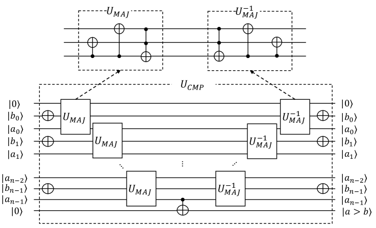
Figure 1: Quantum circuit of $U_{CMP}$.

(4) Again performing Hadamard gate on each qubit of the third register, we yield the state

$$\frac{1}{\sqrt{M}}\sum_{i=0}^{M-1}\left|i\right\rangle\left|\alpha_{i}^{(n)}\right\rangle\left|0\right\rangle^{\otimes n}\left(\frac{\alpha_{i}^{(n)}}{2^{n}}\left|1\right\rangle+\frac{2^{n}-\alpha_{i}^{(n)}}{2^{n}}\left|0\right\rangle\right)+\left|\omega\right\rangle,$$ (13)

where $\left|\omega\right\rangle$, and other states hereafter labeled by $\omega$ with or without subscripts, denote an unnormalized state containing the superposition of nonzero parts in the reference register, if not specified.

(5) Perform the inverse of $O_{AMP}$ to uncompute $\alpha_{i}$ in the second register, and finally measure the last two registers in the state $\left|0\right\rangle^{\otimes n}\left|1\right\rangle$, then the target state 4 is attained in the first register.

The quantum circuit of the whole process is drawn in 2. As shown in 2, the central part of the circuit is constituted by the above steps (2)-(5) apart from the measurement, referred to as amplitude transduction , which is a unitary operation denoted by $U_{AT}$ acting as

$$U_{AT}:\left|i\right\rangle\left|0\right\rangle^{\otimes n}\left|0\right\rangle^{\otimes n}\left|0\right\rangle\mapsto\left|i\right\rangle\left|0\right\rangle^{\otimes n}\left|0\right\rangle^{\otimes n}\left(\frac{\alpha_{i}^{(n)}}{2^{n}}\left|1\right\rangle+\frac{2^{n}-\alpha_{i}^{(n)}}{2^{n}}\left|0\right\rangle\right)+\left|\omega_{i}\right\rangle.$$ (14)

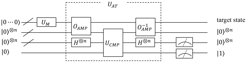
Figure 2: Quantum circuit of arithmetic-free black-box quantum state preparation, where ”/” in the wires indicates a bunch of qubits rather than only one qubit.

3 Quantum algorithm for Gaussian distribution based anomaly detection

As mentioned in section 2.1 and formulated in (2) and (2.1), the goal of GAD is to acquire the mean values $(\mu_{0},\cdots,\mu_{D-1})$ and the covariance matrix $C=(C_{jk})_{D\times D}$ of the multivariate Gaussian distribution used to model the given dataset $\mathcal{D}=\{\bm{x}_{i}=(x_{i0},\cdots,x_{iD-1})|i=0,\cdots,M-1\}$. So, our quantum algorithm consists of two parts: the first one aims to estimate the mean values $\mu_{j}$, while the second one works for estimating covariance matrix elements $C_{jk}$. As explained below, the two parts can be done in almost parallel, while estimating $C_{jk}$ requires the values of $\mu_{j}$ and $\mu_{k}$ as shown in (2.1).

Both parts of our quantum algorithm call for the access to the classical dataset $\mathcal{D}$ on a quantum computer. To accomplish it, we assume that quantum oracles that have access to $\mathcal{D}$ are provided. For convenience, each feature value $x_{ij}$ of each data point $\bm{x}_{i}$ is confined to $x_{ij}\in(-1,1)$, and is stored with precision up to $n$ bits, that is, $2^{n}x_{ij}$ has sign-and-magnitude binary form $x_{ij}:=x_{ij}^{sgn}x_{ij}^{n-1}\cdots x_{ij}^{0}$ with $n+1$ bits, where the first bit $x_{ij}^{sgn}$ is a sign bit with $x_{ij}^{sgn}=0(1)$ indicating non-negative (negative) $x_{ij}$ and the rest bits forms the absolute value of $x_{ij}$. Our algorithms takes two kinds of oracles as follows,

$$O_{j}^{sgn} :\left|i\right\rangle\left|t\right\rangle\mapsto\left|i\right\rangle\left|t\oplus x_{ij}^{sgn}\right\rangle,$$ (15)

$$O_{j}^{abs} :\left|i\right\rangle\left|t\right\rangle\mapsto\left|i\right\rangle\left|t\oplus x_{ij}^{n-1}\cdots x_{ij}^{0}\right\rangle,$$ (16)

for $j=1,2,\cdots,D$, which are to access the sign and the absolute value of $x_{ij}$ of all data points, respectively. In our algorithm, $\left|t\right\rangle$ is set to be $\left|0\right\rangle$, so that $O_{j}^{sgn}$ and $O_{j}^{abs}$ can precisely load the feature values of all the data points in quantum parallel without being affected by the bit of $t$. One way of constructing such oracles is via quantum random access memory (QRAM) [49, 50, 51]. In this case, considering the size of $\mathcal{D}$, performing both $O_{j}^{sgn}$ and $O_{j}^{abs}$ would take time $O(\log(M))$[49, 50, 51]; here we set $n=O(1)$ as its scaling does not depend on the size of $\mathcal{D}$. Moreover, in the NISQ era, it is more favorable to choose the bucket-brigade architecture for QRAM as it is highly resilient to qubit noise[51].

3.1 Part 1: Estimating the mean values

The first part of our quantum algorithm is to estimate all the mean values $\mu_{1},\mu_{2},\cdots,\mu_{D-1}$. For each $\mu_{j}$, our quantum algorithm runs the following steps to estimate it.

(1.1) Prepare five quantum registers with qubits being in the zero states, and then perform the unitary operation $U_{M}$ on the first register to generate the uniform superposition state. This gives the state of all the registers

$$\frac{1}{\sqrt{M}}\sum_{i=0}^{M-1}\left|i\right\rangle\left|0\right\rangle\left|0\right\rangle^{\otimes n}\left|0\right\rangle^{\otimes n}\left|0\right\rangle.$$ (17)

The state corresponds to the initial state (7) of AFBBQSP as described in subsection 2.2, and the first, third, fourth and fifth register are also termed index register, data register, reference register and flag register for the same reason as stated in subsection 2.2. The differences of these two states lie in that the state (17) introduces the second register with one qubit to store the sign of each feature value, called sign register, due to signed feature values of our dataset.

(1.2) Apply the amplitude transduction $U_{AT}$ as shown in 14 with $O_{j}^{abs}$ as the oracle to all the five registers except for the second, so we yield the state

$$\frac{1}{\sqrt{M}}\sum_{i=0}^{M-1}\left|i\right\rangle\left|0\right\rangle\left|0\right\rangle^{\otimes n}\left|0\right\rangle^{\otimes n}\left(\abs{x_{ij}}\left|1\right\rangle+(1-\abs{x_{ij}})\left|0\right\rangle\right)+\left|\omega_{11}\right\rangle.$$ (18)

(1.3) Perform the oracle $O_{j}^{sgn}$ on the first two registers to load the signs of $x_{ij}$ $U_{AT}$ in the second regisiter, the controlled-Z operation on the second register and the last register to make $|x_{ij}|\mapsto x_{ij}$, and the inverse of oracle $O_{j}^{sgn}$ ($O_{j}^{sgn}$ itself) on the first two registers again to uncompute the signs. Now we have the state

$$\frac{1}{\sqrt{M}}\sum_{i=0}^{M-1}\left|i\right\rangle\left|0\right\rangle\left|0\right\rangle^{\otimes n}\left|0\right\rangle^{\otimes n}\left(x_{ij}\left|1\right\rangle+\left(1-\abs{x_{ij}}\right)\left|0\right\rangle\right)+\left|\omega_{12}\right\rangle.$$ (19)

The following two steps (1.4) and (1.4^′) are optional for estimating $\abs{\mu_{j}}$ and the sign of $\mu_{j}$, respectively.

(1.4) Perform the inverse of $U_{M}$ on the first register, and then measure the state of all the five registers to see the outcome $\left|0\right\rangle^{\otimes m}\left|0\right\rangle\left|0\right\rangle^{\otimes n}\left|0\right\rangle^{\otimes n}\left|1\right\rangle$. The success probability of measurement is

$$P_{\mu}=\left(\frac{\sum_{i=0}^{M-1}x_{ij}}{M}\right)^{2}=\mu_{j}^{2},$$ (20)

which gives the estimate of $\abs{\mu_{j}}=\sqrt{P_{\mu}}$.

(1.4^′) Perform the inverse of $U_{M}$ on the first register, and then measure the state of the first four registers to see the outcome $\left|0\right\rangle^{\otimes m}\left|0\right\rangle\left|0\right\rangle^{\otimes n}\left|0\right\rangle^{\otimes n}$ with success probability

$$P_{11}=\left(\frac{\sum_{i=0}^{M-1}x_{ij}}{M}\right)^{2}+\left(\frac{M-\sum_{i=0}^{M-1}\abs{x_{ij}}}{M}\right)^{2}.$$ (21)

The final state of the last flag qubit would be

$$\frac{1}{\sqrt{P_{11}}}\left(\frac{\sum_{i=0}^{M-1}x_{ij}}{M}\left|1\right\rangle+\frac{M-\sum_{i=0}^{M-1}\abs{x_{ij}}}{M}\left|0\right\rangle\right).$$ (22)

Then we perform a Hadamard gate on this state, measure it to see the outcome $\left|1\right\rangle$, and the sign of $\mu_{j}$ is derived with a high probability as explained below.

Thanks to the use of AFBBQSP technique, the step (1.4^′) can acquire the sign of $\mu_{j}$ with a high probability. To see this, we present the technique we call Hadamard sign test (Theorem 3.1) to determine the sign of the product of two real amplitudes in a qubit state $\alpha\left|1\right\rangle+\beta\left|0\right\rangle$ with $\alpha\beta\neq 0$, i.e., the sign of $\alpha\beta$; the proof is provided in A, and the procedure is simple: we just perform a Hadamard operation on this qubit state and measure it to see the outcome $\left|1\right\rangle$. Confining to the state (22) of the flag qubit in step (1.4^′), $\alpha=\frac{\sum_{i=0}^{M-1}x_{ij}}{\sqrt{P_{11}}M}=\frac{\mu_{j}}{\sqrt{P_{11}}}$ and $\beta=\frac{M-\sum_{i=0}^{M-1}\abs{x_{ij}}}{\sqrt{P_{11}}M}$. Since the size of each $x_{ij}$ and each $\abs{x_{ij}}$ generally does not depend on the number of data points $M$ and the number of features $D$, it is natural to assume each $x_{ij},\abs{x_{ij}}\in\mathcal{O}(1)$, then $P_{11}=\mathcal{O}(1)$ and $\alpha,\beta=\mathcal{O}(1)$. Here, we assume the dataset $\mathcal{D}$ is not centered and the size of each mean values relies neither on $M$ nor $D$, that is, each $\mu_{j}\neq 0$ and $\mu_{j}\in\mathcal{O}(1)$. This is reasonable as if each $\mu_{j}=0$ or exponentially approaches to zero, there is no need to estimate the mean values and we can just set $\mu_{j}=0$ and then go straight to estimate the covariance matrix. Therefore, according to Theorem 3.1, the sign of $\alpha\beta$ can be correctly determined with a high probability taking only $\mathcal{O}(1)$ copies of the state (22). Moreover, since $\abs{x_{ij}}<1$, $\beta>0$ always holds, thus the sign of $\alpha$ ($\mu_{j}$) is equal to that of $\alpha\beta$. Therefore, the sign of $\mu_{j}$ can be efficiently determined by taking $O(1)$ copies of the state (22).

[Hadamard sign test] Given a normalized single-qubit state $\left|\varphi\right\rangle=\alpha\left|1\right\rangle+\beta\left|0\right\rangle$ with real amplitudes $\alpha$ and $\beta$ satisfying $\alpha^{2}+\beta^{2}=1$ and $\alpha\beta\neq 0$, there exists a procedure to determine the sign of $\alpha\beta$ with probability greater than or equal to $1-\delta$ using $\mathcal{O}\left(\frac{1}{\delta}\left(\frac{1}{\alpha^{2}}+\frac{1}{\beta^{2}}\right)\right)$ copies of $\left|\varphi\right\rangle$.

The quantum circuit of the whole procedure for estimating $\mu_{j}$, including its absolute value and its sign, is drawn in 3.

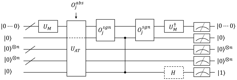
Figure 3: Quantum circuit for estimating each mean value $\mu_{j}$, where $U_{AT}$ is the unitary operation of amplitude transduction defined in 14 that acts on all the registers except for the second one; the dashed line in the $U_{AT}$ box means $U_{AT}$ does not act on the wire of the qubit in the second register. The dashed border line of the last Hadamard operation acting on the last qubit means that the Hadamard operation is operational; it is performed if the quantum circuit is to determine the sign of $\mu_{j}$, while it is not applied if the quantum circuit just runs for estimating the absolute value $\abs{\mu_{j}}$.

It is worthy to note that we can alternatively directly estimate each $\mu_{j}$ instead of estimating $\abs{\mu_{j}}$ and the sign of $\mu_{j}$ separately, by implementing $x_{ij}\leftarrow x_{ij}^{\prime}:=(x_{ij}+1)/2$ which is always greater than zero as $x_{ij}\in(-1,1)$. By doing so, the mean value of $x_{ij}^{\prime}$, denoted by $\mu_{j}^{\prime}=\sum_{i=0}^{M-1}x_{ij}^{\prime}/M=(\mu_{j}+1)/2$, which is also greater than zero and can be directly estimated by the above algorithm in the step (1.4) without determining the sign by the step (1.4^′). This way, $\mu_{j}$ can be obtained as $\mu_{j}=2\mu_{j}^{\prime}-1$. However, implementing $x_{ij}\leftarrow x_{ij}^{\prime}:=(x_{ij}+1)/2$ entails adding a constant on a quantum computer, which would induces additional $O(n)$ qubits and $O(n)$ one- and two-qubit gates when resorting to ripple-carry quantum addition [43], or alternatively uses the quantum Fourier transformation based addition [44, 45, 46, 47] that would introduce additional $O(1)$ qubits and $O(n^{2})$ one- and two-qubit gates. This is unfavorable on NISQ devices as much more quantum resources are required. Therefore, we prefer to estimate $\abs{\mu_{j}}$ and the sign of $\mu_{j}$ in separate.

3.2 Part 2: Estimating the covariance matrix

The second part of our quantum algorithm is to acquire the covariance matrix $C$ of the Gaussian distribution by estimating its each element $C_{jk}$. Since the mean values $\mu_{j}$ are estimated by the first part of our algorithm, the second part only need focus on estimating each

$$C_{jk}^{\prime}: =\frac{\sum_{i=0}^{M-1}x_{ij}x_{ik}}{M-1}$$ (23)

$$=C_{jk}+\frac{M\mu_{j}\mu_{k}}{M-1},$$ (24)

which is derived according to 2.1 and thus $C_{jk}$ can be estimated by estimating $\mu_{j}$ and $C_{jk}^{\prime}$. The following steps are run to estimate each $C_{jk}^{\prime}$.

(2.1) Prepare five quantum registers and run steps (1.1) and (1.2) to create the state (18) .

(2.2) Measure the reference and flag registers to see the outcome $\left|0\right\rangle^{\otimes n}\left|1\right\rangle$, and then the state of the first register would be

$$\frac{1}{\sqrt{MP_{21}}}\sum_{i=0}^{M-1}\abs{x_{ij}}\left|i\right\rangle,$$ (25)

where $P_{21}=\sum_{i=0}^{M-1}x_{ij}^{2}/M$ is the success probability of measurement.

(2.3) Perform Pauli X gate on the old flag qubit to recover its state from $\left|1\right\rangle$ to $\left|0\right\rangle$. Alternatively, we can discard the old reference and flag registers and prepare two new ones in the state $\left|0\right\rangle^{\otimes n}\left|0\right\rangle$. Then again apply $U_{AT}$ with oracle $O_{k}^{abs}$ to all the five registers except for the second one (i.e., the sign qubit). Now we have the state of the whole five registers

$$\frac{1}{\sqrt{MP_{21}}}\sum_{i=0}^{M-1}\abs{x_{ij}}\left|i\right\rangle\left|0\right\rangle\left|0\right\rangle^{\otimes n}\left|0\right\rangle^{\otimes n}\left(\abs{x_{ik}}\left|1\right\rangle+\left(1-\abs{x_{ik}}\right)\left|0\right\rangle\right)+\left|\omega_{21}\right\rangle.$$ (26)

(2.4) Perform oracles $O_{j}^{sgn}$ and $O_{k}^{sgn}$ on the first two registers, controlled-Z operation on the second register, and oracles $O_{k}^{sgn}$ and $O_{j}^{sgn}$ again to load the signs of $x_{ij}$ and $x_{ik}$. This gives the state

$$\frac{1}{\sqrt{MP_{21}}}\sum_{i=0}^{M-1}\left|i\right\rangle\left|0\right\rangle\left|0\right\rangle^{\otimes n}\left|0\right\rangle^{\otimes n}\left(x_{ij}x_{ik}\left|1\right\rangle+\abs{x_{ij}}\left(1-\abs{x_{ik}}\right)\left|0\right\rangle\right)+\left|\omega_{22}\right\rangle.$$ (27)

Similar to the steps (1.4) and (1.4^′), the following steps (2.5) and (2.5^′) run in parallel to estimate $\abs{C_{jk}^{\prime}}$ and the sign of $C_{jk}^{\prime}$, respectively.

(2.5) Same as step (1.4), that is, performing $U_{M}^{\dagger}$ on the first register, and measuring the state of all the five registers to see $\left|0\right\rangle^{\otimes m}\left|0\right\rangle\left|0\right\rangle^{\otimes n}\left|0\right\rangle^{\otimes n}\left|1\right\rangle$. The success probability of measurement is

$$P_{22}=\left(\frac{\sum_{i=0}^{M-1}x_{ij}x_{ik}}{M\sqrt{P_{21}}}\right)^{2},$$ (28)

which gives the estimate of $\abs{C^{\prime}_{jk}}$ as

$$\abs{C^{\prime}_{jk}}=\frac{M\sqrt{P_{21}P_{22}}}{M-1}.$$ (29)

(2.5^′) Same as step (1.5), namely perform $U_{M}^{\dagger}$ on the first register, and measure the state of the first four registers to see the state of zeros. The state of the last flag qubit would be

$$\frac{1}{\sqrt{P_{23}}}\left(\frac{\sum_{i=0}^{M-1}x_{ij}x_{ik}}{M\sqrt{P_{21}}}\left|1\right\rangle+\frac{\sum_{i=0}^{M-1}\abs{x_{ij}}\left(1-\abs{x_{ik}}\right)}{M\sqrt{P_{21}}}\left|0\right\rangle\right),$$ (30)

where

$$P_{23}=\left(\frac{\sum_{i=0}^{M-1}x_{ij}x_{ik}}{M\sqrt{P_{21}}}\right)^{2}+\left(\frac{\sum_{i=0}^{M-1}\abs{x_{ij}}(1-\abs{x_{ik}})}{M\sqrt{P_{21}}}\right)^{2}$$ (31)

represents the success probability of the measurement. Then, as used in the step (1.4^′), the ”Hadamard+measure” trick is applied to retrieve the sign of $C^{\prime}_{jk}$. Note that in the state (30), the sign of the amplitude of $\left|0\right\rangle$ is positive, and the sign of the amplitude of $\left|1\right\rangle$ coincides with that of $C^{\prime}_{jk}$. Thus, according to Theorem 3.1, the sign of $C^{\prime}_{jk}$ can be determined with a high probability. It is worthy to note that, both the matrix $C^{\prime}=(C_{jk}^{\prime})$ and the covariance matrix $C$ are symmetric, and thus only $\frac{D(D+1)}{2}$ rather than $O(D^{2})$ elements of $C^{\prime}$ and $C$ are needed to estimate.

The whole quantum circuit for estimating each $C^{\prime}_{jk}$ is drawn in 4.

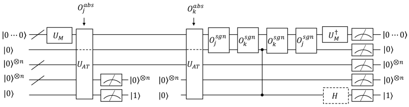
Figure 4: Quantum circuit for estimating each element $C^{\prime}_{jk}$, where the first $U_{AT}$ takes $O_{j}^{abs}$ as the oracle, while the second one takes oracle $O_{k}^{abs}$. Just as 3, the Hadamard operation in the dashed box is applied if this circuit is utilized for retrieving the sign of $C^{\prime}_{jk}$, while it is not applied if the circuit works for estimating $\abs{C^{\prime}_{jk}}$.

4 Complexity analysis

In this section, we individually analyze the time complexity of two parts of our quantum algorithm, and conclude the total time complexity of the whole algorithm.

4.1 Time complexity of estimating mean values

We first analyze the time complexity of estimating $\mu_{j}(j=1,2,\cdots D)$ following the steps (1.1)-(1.4^′) described in 3.1. Step (1.1) involves performing $U_{M}$ which takes time $O[\log(M)]$ as shown in subsection 2.2. Step (1.2) performs amplitude transduction unitary operation $U_{AT}$ whose quantum circuit is drawn in Figure 2, whereas the oracle $O_{AMP}$ in the circuit should be replaced by $O_{j}^{abs}$. Considering $O_{j}^{abs}$ takes time $O[\log(M)]$ and $n=O(1)$ as analyzed above, $U_{AT}$ takes time $O[\log(M)]$. Putting these three together, steps (1.1)-(1.3) takes time $O[\log(M)]$ to generate one copy of the state (19).

As for the step (1.4) for estimating $\abs{\mu_{j}}$, to ensure $\abs{\mu_{j}}$ can be estimated within error $\epsilon_{\mu}$, the error of estimating $P_{\mu}$ has to be within $O\left(\sqrt{P_{\mu}}\epsilon_{\mu}\right)$ according to 20, which results in $O\left[\frac{P_{\mu}(1-P_{\mu})}{P_{\mu}\epsilon_{\mu}^{2}}\right]=O\left(\frac{1}{\epsilon_{\mu}^{2}}\right)$ copies of state (19) are required for measurement in the step (1.4). Thus, $\abs{\mu_{j}}$ can be estimated within error $\epsilon_{\mu}$ in time $O\left[\frac{\log(M)}{\epsilon_{\mu}^{2}}\right]$. It is worthy to note that, the value of $\abs{\mu_{j}}$ significantly less than $\epsilon_{\mu}$ would be estimated to be zero and is unnecessary to proceed to estimate its sign, so only $\abs{\mu_{j}}=\Omega(\epsilon_{\mu})$ matters in the step (1.4^′).

As for the steps (1.1)-(1.3) and (1.4^′) to estimate the sign of $\mu_{j}$, the sign can be correctly determined with probability $\geq 1-\delta$ using $O\left(\frac{1}{\alpha^{2}\beta^{2}\delta}\right)$ copies of the state (22) according to Theorem 3.1. Here,

$$\alpha^{2}=\frac{1}{P_{11}}\left(\frac{\sum_{i=0}^{M-1}x_{ij}}{M}\right)^{2}=\frac{\mu_{j}^{2}}{P_{11}}=\Omega\left(\frac{\epsilon_{\mu}^{2}}{P_{11}}\right)$$ (32)

and

$$\beta^{2}=\frac{1}{P_{11}}\left(\frac{M-\sum_{i=0}^{M-1}\abs{x_{ij}}}{M}\right)^{2}\geq\frac{1}{4^{n}P_{11}},$$ (33)

due to the fact that every $x_{ij}$ lies in (-1,1) with precision up to $n$ bits and $\abs{x_{ij}}\leq 1-\frac{1}{2^{n}}$. This means that $O\left[\frac{P_{11}}{\delta}\left(\frac{1}{\epsilon_{\mu}^{2}}+4^{n}\right)\right]$ copies of the state (22), and hence $O\left[\frac{1}{P_{11}}\frac{P_{11}}{\delta}\left(\frac{1}{\epsilon_{\mu}^{2}}+4^{n}\right)\right]=O\left[\frac{1}{\delta}\left(\frac{1}{\epsilon_{\mu}^{2}}+4^{n}\right)\right]$ copies of the state (19), are required. Therefore, the sign of $\mu_{j}$ can be determined with probability $\geq 1-\delta$ in time $O\left[\frac{\log(M)}{\delta}\left(\frac{1}{\epsilon_{\mu}^{2}}+4^{n}\right)\right]=O\left[\frac{\log(M)}{\epsilon_{\mu}^{2}}\right]$ due to $n,\delta=O(1)$.

Putting above results together, we can conclude that estimating all $D$ mean values $\mu_{1},\mu_{2},\cdots,\mu_{D}$ has time complexity $O\left[\frac{D\log(M)}{\epsilon_{\mu}^{2}}\right]$.

4.2 Time complexity of estimating covariance matrix

The steps (2.1)-(2.5^′) , whose quantum circuit is drawn in 4, are executed to estimate all values $C_{jk}^{\prime}(j,k=1,2,\cdots,D)$, and further estimate all the elements $C_{jk}(j,k=1,2,\cdots,D)$ of the covariance matrix $C$ according to (24). Step (2.1) implements $U_{M}$ and $U_{AT}$, both of which evidently take time $O[\log(M)]$ as analyzed in subsection 4.1. In the step (2.2),suppose $\mathcal{N}$ times of measurement are performed, and consequently $P_{21}$ can be estimated within error

$$O\left[\frac{\sqrt{P_{21}(1-P_{21})}}{\sqrt{\mathcal{N}}}\right],$$

and roughly $\mathcal{N}P_{21}$ copies of the state (25) would be output. Considering $U_{AT}$,$U_{M}^{\ddagger}$, and oracles involved all take time $O[\log(M)]$, the steps (2.3) and (2.4) take time $O[\log(M)]$. In the step (2.5), $P_{22}$ would be estimated with error

$$O\left[\frac{\sqrt{P_{22}(1-P_{22})}}{\sqrt{\mathcal{N}}P_{21}}\right].$$

This results in the error of estimating $\abs{C_{jk}^{\prime}}$ scaling as

$$O\left[\frac{\sqrt{P_{22}}}{\sqrt{P_{21}}}\frac{\sqrt{P_{21}(1-P_{21})}}{\sqrt{\mathcal{N}}}+\frac{\sqrt{P_{21}}}{\sqrt{P_{22}}}\frac{\sqrt{P_{22}(1-P_{22})}}{\sqrt{\mathcal{N}P_{21}}}\right]= O\left[\frac{\sqrt{P_{22}(1-P_{21})}+\sqrt{1-P_{22}}}{\sqrt{\mathcal{N}}}\right]$$ (34)

$$= O\left(\frac{1}{\sqrt{\mathcal{N}}}\right).$$ (35)

Thus, to make the error of estimating $\abs{C_{jk}^{\prime}}$ also be within $O\epsilon_{\mu}$, $\mathcal{N}=O\left(\frac{1}{\epsilon_{\mu}^{2}}\right)$ copies of state (18) are required. This would makes the error of estimating $C_{jk}$ that we denote by $\epsilon_{C}$ less than $3\epsilon$ according to the equation (24). So the total time for estimating the absolute values of all the elements (i.e., $\abs{C_{jk}}$) of the covariance matrix $C$ within error $\mathcal{O}(\epsilon_{\mu})$ scales as $\mathcal{O}\left[\frac{D^{2}\log(M)}{\epsilon_{\mu}^{2}}\right]$, provided that we have already acquired the the estimates of all $\mu_{j}$ and that the time for preparing the state (18) scales as $\mathcal{O}(\log(M))$ as shown in subsection 4.1.

Now we analyze the time complexity for estimating the sign of $C_{jk}^{\prime}$. Similar to estimating the sign of mean values $\mu_{j}$, only if the magnitude of $C_{jk}^{\prime}$ is significantly large, i.e., $\abs{C_{jk}^{\prime}}=\Omega(\epsilon_{\mu})$, it is necessary to run the steps (2.1)-(2.4) and (2.5^′) to estimate the sign of $C_{jk}^{\prime}$. As shown in the step (2.5^′), according to Theorem 3.1, $O\left[\frac{1}{\delta}(\frac{1}{\alpha^{2}}+\frac{1}{\beta^{2}})\right]$ copies of the state (30) are taken to ensure the sign of $C_{jk}^{\prime}$ can be correctly determined with probability $\geq 1-\delta$. Here

$$\alpha^{2}=\frac{1}{P_{21}P_{23}}\left(\frac{\sum_{i=0}^{M-1}x_{ij}x_{ik}}{M}\right)^{2}\approx\frac{C_{jk}^{\prime 2}}{P_{21}P_{23}}=\Omega\left(\frac{\epsilon_{\mu}^{2}}{P_{21}P_{23}}\right)$$ (36)

and

$$\beta^{2} =\frac{1}{P_{21}P_{23}}\left(\frac{\sum_{i=0}^{M-1}\abs{x_{ij}}(1-\abs{x_{ik}})}{M}\right)^{2}$$

$$\geq\frac{1}{P_{21}P_{23}}\left(\frac{\sum_{i=0}^{M-1}\abs{x_{ij}}}{2^{n}M}\right)^{2}$$

$$\geq\frac{\mu_{j}^{2}}{P_{21}P_{23}4^{n}}=\Omega\left(\frac{\epsilon_{\mu}^{2}}{P_{21}P_{23}4^{n}}\right).$$ (37)

As a result, $O\left[\frac{P_{21}P_{23}}{\delta}\left(\frac{1}{\epsilon_{\mu}^{2}}+\frac{4^{n}}{\epsilon_{\mu}^{2}}\right)\right]$ copies of the state (30), and thus also $O\left[\frac{1}{\delta}\left(\frac{1}{\epsilon_{\mu}^{2}}+\frac{4^{n}}{\epsilon_{\mu}^{2}}\right)\right]=O\left[\frac{1}{\epsilon_{\mu}^{2}}\right]$ copies of the state (18) in the step (2.1), are sufficient. Therefore, the time for estimating the sign of each $C_{jk}^{\prime}$ scales as $O\left[\frac{\log(M)}{\epsilon_{\mu}^{2}}\right]$, which is same as that of estimating all $\abs{C_{jk}^{\prime}}$, and gives the overall time complexity for estimating all the elements of the covariance matrix $C$ being $O\left[\frac{D^{2}\log(M)}{\epsilon_{\mu}^{2}}\right]$. It is not hard to see that the time for estimating the covariance matrix $C$ is much larger than that for estimating all $D$ mean values $\bm{\mu}$, and thus the whole time complexity of the proposed quantum algorithm for GAD is

$$\mathcal{O}\left(\frac{D^{2}\log(M)}{\epsilon_{\mu}^{2}}\right).$$ (38)

4.3 Time complexity of the whole algorithm

Keeping in mind that the ultimate goal of our quantum algorithm is to estimate the probability $p(\bm{x})$ (equation (1)), the overall time complexity of our quantum algorithm depends on the error of estimating $p(\bm{x})$. Hence, it is necessary to see how this error is affected by the errors of estimating $\mu_{j}$ and $C_{jk}$, i.e., $\epsilon_{\mu}$ and $\epsilon_{C}$. For convenience, we use $\Delta Q:=\hat{Q}-Q$ to denote the difference between the estimate of a quantity $Q$ denoted by $\hat{Q}$; the error of estimating $p(\bm{x})$ would be $\abs{\Delta p(\bm{x})}$ . Following this definition, it is easy to see $\Delta\bm{\mu}=\hat{\bm{\mu}}-\bm{\mu}$ would be a column vector with elements being $\hat{\mu}_{j}-\mu_{j}\leq\epsilon_{\mu}$ and $\Delta C=\hat{C}-C$ would be a matrix with elements being $\hat{C}_{jk}-C_{jk}\leq\epsilon_{C}$. According to the equation (1), $\abs{\Delta p(\bm{x})}$ is upper bounded by

$$\abs{\Delta p(\bm{x})} =\abs{\Delta(e^{\ln p(\bm{x})})}$$ (39)

$$\approx p(\bm{x})\abs{\Delta(\ln p(\bm{x}))}$$ (40)

$$\leq\abs{\Delta(\ln p(\bm{x}))}$$ (41)

$$=\frac{1}{2}\abs{\Delta(\ln\abs{C})+\Delta\left((\bm{x}-\bm{\mu})^{\top}C^{-1}(\bm{x}-\bm{\mu})\right)}$$ (42)

$$\leq\frac{1}{2}\abs{\Delta(\ln\abs{C})}+\frac{1}{2}\abs{\Delta\left((\bm{x}-\bm{\mu})^{\top}C^{-1}(\bm{x}-\bm{\mu})\right)}.$$ (43)

Next, we individually analyze the upper bound of $\abs{\Delta(\ln\abs{C})}$ and that of $\abs{\Delta\left((\bm{x}-\bm{\mu})^{\top}C^{-1}(\bm{x}-\bm{\mu})\right)}$. According to the determinant relative error bound [52], the former one can be derived as

$$\abs{\Delta(\ln\abs{C})} \approx\abs{\frac{\abs{\hat{C}}-\abs{C}}{\abs{C}}}$$ (44)

$$\leq\frac{D\left\lVert C^{-1}\right\rVert\left\lVert\Delta C\right\rVert}{1-D\left\lVert C^{-1}\right\rVert\left\lVert\Delta C\right\rVert}$$ (45)

$$\leq 2D\left\lVert C^{-1}\right\rVert\left\lVert\Delta C\right\rVert,$$ (46)

provided that $D\left\lVert C^{-1}\right\rVert\left\lVert\Delta C\right\rVert\leq 1/2<1$. Here $\left\lVert\bullet\right\rVert$ stands for the 2-norm of a vector or the $L_{2}$ norm of a matrix. Letting $\bm{y}:=\bm{x}-\bm{\mu}$ and $\hat{\bm{y}}:=\bm{x}-\hat{\bm{\mu}}$, we have

$$\abs{\Delta\left((\bm{x}-\bm{\mu})^{\top}C^{-1}(\bm{x}-\bm{\mu})\right)} =\abs{(\bm{x}-\bm{\mu})^{\top}C^{-1}(\bm{x}-\bm{\mu})-(\bm{x}-\hat{\bm{\mu}})^{\top}\hat{C}^{-1}(\bm{x}-\hat{\bm{\mu}})}$$ (47)

$$=\abs{\bm{y}^{\top}C^{-1}\bm{y}-\hat{\bm{y}}^{\top}\hat{C}^{-1}\hat{\bm{y}}}$$ (48)

$$=\abs{\bm{y}^{\top}C^{-1}\bm{y}-\bm{y}^{\top}\hat{C}^{-1}\hat{\bm{y}}+\bm{y}^{\top}\hat{C}^{-1}\hat{\bm{y}}-\hat{\bm{y}}^{\top}\hat{C}^{-1}\hat{\bm{y}}}$$ (49)

$$\leq\abs{\bm{y}^{\top}C^{-1}\bm{y}-\bm{y}^{\top}\hat{C}^{-1}\hat{\bm{y}}}+\abs{\bm{y}^{\top}\hat{C}^{-1}\hat{\bm{y}}-\hat{\bm{y}}^{\top}\hat{C}^{-1}\hat{\bm{y}}}$$ (50)

$$\leq\left\lVert\bm{y}\right\rVert\left\lVert C^{-1}\bm{y}-\hat{C}^{-1}\hat{\bm{y}}\right\rVert+\left\lVert\bm{y}-\hat{\bm{y}}\right\rVert\left\lVert\hat{C}^{-1}\hat{\bm{y}}\right\rVert$$ (51)

$$\leq\left\lVert\bm{y}\right\rVert\left\lVert\hat{C}^{-1}\right\rVert(\left\lVert\hat{\bm{y}}-\bm{y}\right\rVert+\left\lVert\Delta C\right\rVert\left\lVert C^{-1}\right\rVert\left\lVert\bm{y}\right\rVert)+\left\lVert\bm{y}-\hat{\bm{y}}\right\rVert\left\lVert\hat{C}^{-1}\right\rVert\left\lVert\hat{\bm{y}}\right\rVert$$ (52)

$$=\left\lVert\hat{C}^{-1}\right\rVert\left\lVert\hat{\bm{y}}-\bm{y}\right\rVert(\left\lVert\bm{y}\right\rVert+\left\lVert\hat{\bm{y}}\right\rVert)+\left\lVert\hat{C}^{-1}\right\rVert\left\lVert C^{-1}\right\rVert\left\lVert\Delta C\right\rVert\left\lVert\bm{y}\right\rVert^{2}$$ (53)

$$\leq 2\left\lVert C^{-1}\right\rVert\left\lVert\hat{\bm{y}}-\bm{y}\right\rVert(\left\lVert\bm{y}\right\rVert+\left\lVert\hat{\bm{y}}\right\rVert)+2\left\lVert C^{-1}\right\rVert^{2}\left\lVert\Delta C\right\rVert\left\lVert\bm{y}\right\rVert^{2},$$ (54)

where the above inequality (53) holds due to the fact that $\hat{C}^{-1}\hat{\bm{y}}-C^{-1}\bm{y}=\hat{C}^{-1}(\hat{\bm{y}}-\bm{y}-\Delta CC^{-1}\bm{y})$ , and the inequality (54) holds as $\left\lVert\hat{C}^{-1}\right\rVert\leq\left\lVert C^{-1}\right\rVert/(1-\left\lVert\Delta CC^{-1}\right\rVert)\leq 2\left\lVert C^{-1}\right\rVert$ for $\left\lVert\Delta CC^{-1}\right\rVert\leq\left\lVert C^{-1}\right\rVert\left\lVert\Delta C\right\rVert\leq D\left\lVert C^{-1}\right\rVert\left\lVert\Delta C\right\rVert\leq 1/2$; the results can be seen in [53].

Putting the inequalities (43),(46) and (54) together, we have

$$\abs{\Delta p(\bm{x})} \leq D\left\lVert C^{-1}\right\rVert\left\lVert\Delta C\right\rVert+\left\lVert C^{-1}\right\rVert\left\lVert\hat{\bm{y}}-\bm{y}\right\rVert(\left\lVert\bm{y}\right\rVert+\left\lVert\hat{\bm{y}}\right\rVert)+\left\lVert C^{-1}\right\rVert^{2}\left\lVert\Delta C\right\rVert\left\lVert\bm{y}\right\rVert^{2}$$ (55)

$$\leq D^{2}\left\lVert C^{-1}\right\rVert\epsilon_{C}+4D\left\lVert C^{-1}\right\rVert\epsilon_{\mu}+4D^{2}\left\lVert C^{-1}\right\rVert^{2}\epsilon_{C}$$ (56)

$$\leq 3D^{2}\left\lVert C^{-1}\right\rVert\epsilon_{\mu}+4D\left\lVert C^{-1}\right\rVert\epsilon_{\mu}+12D^{2}\left\lVert C^{-1}\right\rVert^{2}\epsilon_{\mu}$$ (57)

$$\leq 7D^{2}\left\lVert C^{-1}\right\rVert\epsilon_{\mu}+12D^{2}\left\lVert C^{-1}\right\rVert^{2}\epsilon_{\mu}.$$ (58)

Here the inequality (56) holds as the absolute value of each element of $\Delta C$ is within $\epsilon_{C}$ and $\left\lVert\Delta C\right\rVert\leq D\epsilon_{C}$, the absolute value of each element of $\hat{\bm{y}}-\bm{y}$ is within $\epsilon_{\mu}$ and $\left\lVert\hat{\bm{y}}-\bm{y}\right\rVert\leq\sqrt{D}\epsilon_{\mu}$, and each element of $\bm{y}$ and $\hat{\bm{y}}$ lies in $(-2,2)$ and thus $\left\lVert\hat{\bm{y}}\right\rVert,\left\lVert\bm{y}\right\rVert\leq 2\sqrt{D}$. The inequality (57) holds due to $\epsilon_{C}\leq 3\epsilon_{\mu}$ as analyzed above, and the inequality (58) is derived for $4D\left\lVert C^{-1}\right\rVert\epsilon_{\mu}\leq 4D^{2}\left\lVert C^{-1}\right\rVert\epsilon_{\mu}$. In order to make $p(\bm{x})$ be estimated within error $\epsilon$, i.e., $\abs{\Delta p(\bm{x})}\leq\epsilon$, we set $\epsilon_{\mu}=\epsilon/(7D^{2}\left\lVert C^{-1}\right\rVert+12D^{2}\left\lVert C^{-1}\right\rVert^{2})$ as implied by the inequality (58). Furthermore, since $\left\lVert C\right\rVert$ corresponds to the largest eigenvalue for the positive definite matrix $C$ and satisfy $\left\lVert C\right\rVert=\left\lVert\frac{X(\mathbb{I}-\left|\bm{e}\rangle\langle\bm{e}\right|)X^{\top}}{M-1}\equiv(C_{jk})_{D\times D}\right\rVert\leq\frac{\left\lVert X\right\rVert\left\lVert\mathbb{I}-\left|\bm{e}\rangle\langle\bm{e}\right|\right\rVert\left\lVert X^{\top}\right\rVert}{M-1}=\frac{\left\lVert X\right\rVert\left\lVert X^{\top}\right\rVert}{M-1}\leq D$, we let the eigenvalues of $C$ lie in $[D/\kappa,D]$, where $\kappa$ is an effective condition number of $C$ that upper bounds its actual condition number. Consequently, $\left\lVert C^{-1}\right\rVert\leq\kappa/D$,

$$\frac{1}{\epsilon_{\mu}}\leq\frac{7D\kappa+12\kappa^{2}}{\epsilon},$$ (59)

and the overall time complexity of our quantum algorithm for estimating $p(\bm{x})$ within error $\epsilon$ according to the equation (38) is

$$\mathcal{O}\left(\frac{D^{2}\kappa^{2}(D+\kappa)^{2}\log(M)}{\epsilon^{2}}\right).$$ (60)

5 Discussion

In this section, we discuss the advantages of the proposed qGAD algorithm over the classical algorithm or the prior qGAD algorithms. Comparison between the proposed qGAD algorithm and the classical GAD algorithm and the prior qGAD algorithms is listed in the table 1, from which we conclude advantages of the proposed qGAD algorithm from the aspects of quantum circuit depth, practicality, and efficiency shown below.

5.1 Quantum circuit depth

Our algorithm builds on the technique of AFQSP whose quantum circuit depth is linear with the qubit count, whereas the prior qGAD algorithms [36, 37] take the technique of amplitude estimation as key subroutines and may has depth exponential with the number of used qubits. Since shallower quantum circuit usually means less opportunity for errors to occur, the proposed algorithm is more suitable to implement on NISQ devices.

5.2 Practicality on data

The prior qGAD algorithms suffer from at least one of the three restrictions for input data: (a) the vector of each data point is required to be normalized and presented in a quantum state (i.e., quantum data) [36]; (b) the data is required to be mean centered which means each $\mu_{j}=0$ [36]; (c) each data feature is required to be uncorrelated with others which implies the correlation matrix $C$ is a diagonal matrix [37]. In contrast, our algorithm releases these restrictions and handle classical, mean centered/uncenterd and feature correlated/uncorrelated data, which occur much more frequently in the real world. In this sense, the proposed qGAD algorithm is more practical.

5.3 Efficiency

From table 1, it is easy to see the proposed qGAD algorithm has time complexity $\mathcal{O}\left(\mathrm{polylog}\left(M\right)\right)$ when $D,\kappa,1/\epsilon=\mathcal{O}(\mathrm{polylog}\left(M\right))$, while the classical GAD algorithm takes time complexity $\mathcal{O}(M\mathrm{polylog}\left(M\right))$ under the same conditions. This means that the proposed qGAD algorithm has potential to achieve exponential speedup over the classical GAD under certain conditions. However, it is unfair to compare the current time complexity of the proposed qGAD algorithm with that of the prior qGAD algorithms [36, 37] because they are derived based on different assumptions on input data as analyzed above, though it seems that the proposed algorithm has time complexity with better dependence on $\epsilon$ but worse on $D$ and $\kappa$ when compared with the qGAD algorithm [37].

One may concern if the proposed qGAD algorithm can be dequantized by the technique of quantum-inspired classical sampling, which has made many QML or QML related algorithms, such as quantum algorithm for recommendation systems [54], quantum principal component analysis [55], quantum clustering [55], quantum linear regression [56], and so on, lose exponential speedups over their classical counterparts. An overview of quantum-inspired classical algorithms can be seen in [57, 58]. Given a dataset of data points (vectors) $\{\mathbf{x}_{i}|i=0,1,\cdots,M-1\}$, most existing QML algorithms assume there is a efficient procedure to create $\left|\mathbf{x}_{i}\right\rangle$ for every data vector $\mathbf{x}_{i}$ and the states of all the data points $\left|\mathbf{x}_{i}\right\rangle$ together with the norms $\left\lVert\mathbf{x}_{i}\right\rVert$ can be efficiently accessed in quantum parallel via quantum oracles. The quantum oracles can be by QRAM provided a special data structure in which subsets of sums of squared data vector entries are stored in a binary tree [54, 58]. To make the classical counterparts more comparable to QML algorithms, quantum-inspired algorithms assume an analogous quantum-inspired input data model, i.e., sampling and query (SQ) access to a vector or a matrix. More specifically, $\mathrm{SQ}(\mathbf{v})$, sampling and query access to a column vector $\mathbf{v}=(v_{0},v_{1},\cdots,v_{M-1})^{\top}\in\mathbb{C}^{M}$, supports three efficient operations: (i) querying for $v_{i}$ for all $i=0,1,\cdots,D-1$; (ii) sampling $v_{i}$ with probability $v_{i}^{2}/\left\lVert\mathbf{v}\right\rVert^{2}$; (iii) querying for $\left\lVert\mathbf{v}\right\rVert$. The SQ model allows efficient estimation of inner product, singular value transformation, matrix-vector multiplication and so on [58]. Let us take inner product estimation as an example. Given $\mathrm{SQ}(\mathbf{u})$ and $\mathrm{SQ}(\mathbf{v})$ for two vectors $\mathbf{u},\mathbf{v}\in\mathbb{C}^{M}$, one can efficiently estimate the inner product $\mathbf{u}^{\top}\mathbf{v}$ within additive error $\left\lVert\mathbf{u}\right\rVert\left\lVert\mathbf{v}\right\rVert\epsilon$ with at least $1-\delta$ probability using only $\mathcal{O}\left(\frac{1}{\epsilon^{2}}\log\left(\frac{1}{\delta}\right)\right)$ queries and samplings, which is independent of the dimensionality $M$.

As for our qGAD algorithm, efficient estimating inner product is crucial because each mean value $\mu_{j}=\mathbf{e}^{\top}\mathbf{x}_{\cdot j}/M$ and each $C^{\prime}_{jk}=\mathbf{x}_{\cdot j}^{\top}\mathbf{x}_{\cdot k}$ can be seen as the inner product of two vectors, where $\mathbf{x}_{\cdot j}=(x_{0j},x_{1j},\cdots,x_{M-1j})$ represents a column vector of $(j+1)$th feature values of all $M$ data points. If we have $\mathrm{SQ}(\mathbf{x}_{\cdot j})$ for all $j=0,1,\cdots,D-1$, we can efficiently estimate each $\mu_{j}$ and each $C^{\prime}_{jk}$ in time independent of $M$, which would ruin the exponential speedup potential of the proposed qGAD algorithm over the classical GAD algorithm. However, as shown in the equations (15) and (16), the proposed algorithm only assume quantum access to each entry of all data points $\mathbf{x}_{i}$, neither their quantum states $\left|\mathbf{x}_{.j}\right\rangle$ nor the norms $\left\lVert\mathbf{x}_{\cdot j}\right\rVert$. This means it is reasonable to assume the operation (i), while the operations (ii) and (iii) do not apply. Without operations (ii) and (iii), quantum-inspired classical sampling technique cannot efficiently estimate the inner product of any two vectors [54, 58]. Therefore, SQ data access model is not an appropriate analogy of the input data model in our qGAD algorithm, and thus our algorithm is resilient against quantum-inspired classical sampling.

Table 1: Comparison between the proposed qGAD algorithms and the classical algorithm and other prior qGAD algorithms, where / means the classical GAD has no quantum circuit depth.

Algorithms	Data type	Mean centered	Features correlated	Quantum circuit depth	Time complexity
Classical GAD	Classical	Not required	Not required	/	$\mathcal{O}(D^{2}(M+D))$
qGAD[36]	Quantum	Required	Not required	Exponential	$\Omega\left(\frac{\log(MD)\kappa^{2}}{\epsilon}\right)$
qGAD[37]	Classical	Not required	Required	Exponential	$\mathcal{O}\left(\frac{\log(MD)D^{3}}{\epsilon^{3}}\right)$
The proposed qGAD	Classical	Not required	Not required	Linear	$\mathcal{O}\left(\frac{D^{2}\kappa^{2}(D+\kappa)^{2}\log(M)}{\epsilon^{2}}\right)$

6 Conculsions

To address the high quantum circuit depth of existing quantum Gaussian-based Anomaly Detection (GAD) algorithms, which limits their efficient implementation on NISQ devices, this work proposes a novel quantum GAD algorithm. The results demonstrate that, compared to existing quantum algorithms, the proposed algorithm reduces the circuit depth from exponential($O(2^{n})$) to linear($O(n)$) scaling. Furthermore, it achieves exponential speedup in the number of data samples compared to classical counterparts. While a wide variety of anomaly detection algorithms have demonstrated strong performance in classical computing and hold potential for quantum extensions, research in this direction remains limited. The proposed quantum GAD algorithm is expected to inspire further exploration into quantum acceleration for anomaly detection tasks.

This work is supported by National Natural Science Foundation of China (Grant Nos. 62006105,62301454), China Postdoctoral Science Foundation (Grant No. 2023M731429), Jiangxi Provincial Natural Science Foundation (Grant No. 20202BABL212004), Fundamental Research Funds for the Central Universities (Grant No. SWU-KQ22049), and the Natural Science Foundation of Chongqing (Grant No. CSTB2023NSCQ-MSX0739)

Appendix A Proof of Theorem 1

Given a normalized single-qubit state $\left|\varphi\right\rangle=\alpha\left|1\right\rangle+\beta\left|0\right\rangle$ with real amplitudes $\alpha$ and $\beta$ and with $\alpha^{2}+\beta^{2}=1$, one can implement the “Hadamard+measure” procedure to determine the sign of $\alpha\beta$, that is, to determine whether $\alpha\beta\geq 0$ or $\alpha\beta<0$. Specifically, one can perform a Hadamard gate on this qubit, and then measure it $N_{s}$ times to see the outcome $\left|1\right\rangle$ with success probability $P_{s}:=\frac{1}{2}-\alpha\beta$. Letting $\hat{P}_{s}$ denote the actual proportion of getting the outcome $\left|1\right\rangle$, if $\hat{P}_{s}\leq 1/2$, $\alpha\beta\geq 0$ holds; otherwise, we believe $\alpha\beta<0$.

Now we analyze the scaling of $N_{s}$ when we want to correctly acquire the sign of $\alpha\beta$ with a probability greater than or equal to $1-\delta$. As we know, $N_{s}\hat{P}_{s}$ is a random variable in the binomial distribution $B(N_{s},P_{s})$, so $\hat{P}_{s}$ has expected value $\mathbb{E}(\hat{P}_{s})=\frac{1}{2}-\alpha\beta$ and variance $\frac{\frac{1}{4}-\alpha^{2}\beta^{2}}{N_{s}}$. Consider two cases: $\alpha\beta\geq 0$ and $\alpha\beta<0$. For the former case with $\alpha\beta\geq 0$, the probability of getting the right sign of $\alpha\beta$ is

$$\mathrm{Prob}\left(\hat{P}_{s}\leq 1/2\right) =\mathrm{Prob}\left(\hat{P}_{s}-\mathbb{E}(\hat{P}_{s})\leq\alpha\beta\right)$$ (61)

$$=1-\mathrm{Prob}\left(\hat{P}_{s}-\mathbb{E}(\hat{P}_{s})>\alpha\beta\right)$$ (62)

$$\geq 1-\frac{\frac{1}{4}-\alpha^{2}\beta^{2}}{\frac{1}{4}-\alpha^{2}\beta^{2}+N_{s}\alpha^{2}\beta^{2}},$$ (63)

due to Cantelli inequality. So, if we require the probability to be greater than or equal to $1-\delta$, $N_{s}$ should satisfy

$$N_{s}\geq\frac{(1-\delta)(1-4\alpha^{2}\beta^{2})}{4\delta\alpha^{2}\beta^{2}}.$$ (64)

Thus, $N_{s}=\mathcal{O}\left(\frac{1}{\delta}\left(\frac{1}{\alpha^{2}}+\frac{1}{\beta^{2}}\right)\right)$ is sufficient.

For the other case $\alpha\beta<0$, the sign of $\alpha\beta$ is acquired correctly with probability

$$\mathrm{Prob}\left(\hat{P}_{s}>1/2\right) =\mathrm{Prob}\left(\hat{P}_{s}-\mathbb{E}(\hat{P}_{s})>\alpha\beta\right)$$ (65)

$$=1-\mathrm{Prob}\left(\hat{P}_{s}-\mathbb{E}(\hat{P}_{s})\leq\alpha\beta\right),$$ (66)

which would give rise to the same inequalities as (63) and (64) according to Cantelli inequality.

Putting the above two cases together, the sign of $\alpha\beta$ can be determined with probability $\geq 1-\delta$ using $\mathcal{O}\left(\frac{1}{\delta}\left(\frac{1}{\alpha^{2}}+\frac{1}{\beta^{2}}\right)\right)$ copies of $\left|\varphi\right\rangle$.

References

- [1] P. W. Shor, Algorithms for quantum computation: Discrete logarithms and factoring, in Proceedings of the 35th Annual Symposium on the Foundations of Computer Science, edited by S. Goldwasser (IEEE, Los Alamitos, California, 1994), pp.124–134.
- [2] L. K. Grover, Quantum mechanics helps in searching for a needle in a haystack, Phys. Rev. Lett. 79, 325 (1997).
- [3] A. W. Harrow, A. Hassidim, and S. Lloyd, Quantum algorithm for linear systems of equations, Phys. Rev. Lett. 103, 150502 (2009).
- [4] J. Biamonte, P. Wittek, N. Pancotti, P. Rebentrost, N. Wiebe, and S. Lloyd, Quantum machine learning, Nature 549, 195–202 (2017).
- [5] S. Lloyd, M. Mohseni, P. Rebentrost, Quantum algorithms for supervised and unsupervised machine learning, arXiv:1307.0411, 2013.
- [6] K. L. Pudenz and D. A. Lidar, Quantum adiabatic machine learning, Quantum Inf. Process. 12, 2027 (2013).
- [7] P. Rebentrost, M. Mohseni, S. Lloyd, Quantum support vector machine for big data classification, Phys. Rev. Lett. 113, 130503 (2014).
- [8] I. Cong, L. Duan, Quantum discriminant analysis for dimensionality reduction and classification, New J. Phys. 18, 073011 (2016).
- [9] M. Schuld, M. Fingerhuth and F. Petruccione, Implementing a distance-based classifier with a q uantum interference circuit, Europhysics Letters 119, 60002 (2017).
- [10] Schuld and F. Petruccione, Quantum ensembles of quantum classifiers, Sc. Rep. 8, 2772 (2018).
- [11] M. Schuld and N. Killoran, Quantum machine learning in feature Hilbert spaces, Phys. Rev. Lett. 122, 040504 (2019).
- [12] V. Havlíĉek, A. D. Córcoles, K. Temme1, A. W. Harrow, A. Kandala, J. M. Chow, and Jay M. Gambetta, Supervised learning with quantum-enhanced feature spaces, Nature 567, 209 (2019).
- [13] Y. Song, J. Li, Y. Wu, S. Qin, Q. Wen, and F. Gao, A resource-efficient quantum convolutional neural network, Front Phys 12, 1362690 (2024).
- [14] E. Aimeur, G. Brassard, S. Gambs, Quantum speed-up for unsupervised learning, Mach. Learn. 90, 261 (2013).
- [15] Davis Arthur and Prasanna Date, Balanced k-means clustering on an adiabatic quantum computer, Quantum Information Processing 20, 294 (2021).
- [16] Z. Wu, T. Song, and Y. Zhang, Quantum k-means algorithm based on Manhattan distance, Quantum Information Processing 21, 19 (2022).
- [17] N.Wiebe, D. Braun, S. Lloyd, Quantum algorithm for data fitting, Phys. Rev. Lett. 109, 050505 (2012).
- [18] M. Schuld, I. Sinayskiy, F. Petruccione, Prediction by linear regression on a quantum computer, Phys. Rev. A 94, 022342 (2016).
- [19] G. Wang, Quantum algorithm for linear regression, Phys. Rev. A 96, 012335 (2017).
- [20] Y. Liu and S. Zhang, Fast quantum algorithms for least squares regression and statistic leverage scores, Theor. Comput. Sci. 657, 38 (2017).
- [21] C.-H. Yu, F. Gao, C. Liu, D. Huynh, M. Reynolds, and J. Wang, Quantum algorithm for visual tracking, Phys. Rev. A 99, 022301 (2019).
- [22] C.-H. Yu, F. Gao, and Q.-Y. Wen. An improved quantum algorithm for ridge regression, IEEE Trans Knowl Data Eng 33, 858 (2021).
- [23] C.-H. Yu, F. Gao, Q.-L. Wang, and Q.-Y. Wen, Quantum algorithm for association rules mining, Phys. Rev. A 94, 042311 (2016).
- [24] C.-H. Yu. Experimental implementation of quantum algorithm for association rules mining. IEEE J Emerging Sel Top Circuits Syst, 12, 676-684 (2022).
- [25] S. Lloyd, M. Mohseni, P. Rebentrost, Quantum principal component analysis, Nat. Phys. 10, 631 (2014).
- [26] C.-H. Yu, F. Gao, S. Lin, and J. Wang, Quantum data compression by principal component analysis, Quantum Information Processing 18, 249 (2019).
- [27] B. Duan, J. Yuan, J. Xu, and D. Li, Quantum algorithm and quantum circuit for A-optimal projection: Dimensionality reduction, Phys. Rev. A 99, 032311 (2019).
- [28] A. Sornsaeng, N. Dangniam, P. Palittapongarnpim, and T. Chotibut, Quantum diffusion map for nonlinear dimensionality reduction, Phys. Rev. A 104, 052410 (2021).
- [29] V. Chandola, A. Banerjee, and V. Kumar, Anomaly detection: A survey, ACM Comput. Surv. 41(3), 1–58 (2009).
- [30] W. Hilal, S. A. Gadsden, and J. Yawney, Financial fraud: a review of anomaly detection techniques and recent advances, Expert Syst. Appl. 193, 116429 (2022).
- [31] Z. Ahmad, A. Shahid Khan, C. Wai Shiang, and F. Ahmad, Network intrusion detection system: A systematic study of machine learning and deep learning approaches, Trans. Emerging Telecommun. Technol. 32(1), e4150 (2021).
- [32] T. Fernando, H. Gammulle, S. Denman, S. Sridharan, and C. Fookes, Deep learning for medical anomaly detection–a survey, ACM Comput. Surv. 54(7), 1–37 (2021).
- [33] P.-N. Tan, M. Steinbach, and V. Kumar, Introduction to data mining (Pearson Education India, 2016).
- [34] S. Corli, L. Moro, D. Dragoni, M. Dispenza, and E. Prati, Quantum machine learning algorithms for anomaly detection: A review, Future Gener. Comput. Syst, 107632 (2024).
- [35] N. Liu and P. Rebentrost, Quantum machine learning for quantum anomaly detection, Phys. Rev. A 97(4), 042315 (2018).
- [36] J. M. Liang, S. Q. Shen, M. Li, and L. Li, Quantum anomaly detection with density estimation and multivariate Gaussian distribution, Phys. Rev. A 99(5), 052310 (2019).
- [37] M. Guo, H. Liu, Y. Li, W. Li, F. Gao, S. Qin and Q. Wen, Quantum algorithms for anomaly detection using amplitude estimation, Physica A 604, 127936 (2022).
- [38] M. C. Guo, H. L. Liu, S. J. Pan, W. M. Li, F. Gao, X. Y. Huang, and Q. Y. Wen, Quantum Algorithm for Anomaly Detection of Sequences, Adv. Quantum Technol. 6(8), 2300082 (2023).
- [39] M. Guo, S. Pan, W. Li, F. Gao, S. Qin, X. Yu, and Q. Wen, Quantum algorithm for unsupervised anomaly detection, Physica A 625, 129018 (2023).
- [40] H. M. Rao, C. H. Yu, Y. P. Wu, D. X. Liu, and X. P. Liu, Quantum algorithm for angle-based anomaly detection, Sci. Sin. Phys. Mech. Astron. 55(4), 240307 (2025).
- [41] J. Preskill, Quantum computing in the NISQ era and beyond, Quantum 2, 79 (2018).
- [42] Y. R. Sanders, G. H. Low, A. Scherer, and D. W. Berry, Black-Box Quantum State Preparation without Arithmetic, Phys. Rev. Lett. 122, 020502 (2019).
- [43] S. A. Cuccaro, T. G. Draper, S. A. Kutin, and D. P. Moulton, A new quantum ripple-carry addition circuit, arXiv:quant-ph/0410184 (2004).
- [44] T. G. Draper, Addition on a Quantum Computer, arXiv:quant-ph/0008033 (2000).
- [45] L. Ruiz-Perez , and J. C. Garcia-Escartin, Quantum arithmetic with the quantum Fourier transform, Quantum Inf. Process. 16, 152 (2017).
- [46] E. Şahin, Quantum arithmetic operations based on quantum Fourier transform on signed integers, Int. J. Quantum Inf. 18, 2050035 (2020).
- [47] F C. Ferraz, Quantum algorithm based on quantum Fourier transform for register-by-constant addition, arXiv:2207.05309 (2022).
- [48] L. K. Grover, Synthesis of Quantum Superpositions by Quantum Computation, Phys. Rev. Lett. 85, 1334 (2000).
- [49] V. Giovannetti, S. Lloyd, and L. Maccone, Quantum random access memory, Phys. Rev. Lett. 100, 160501 (2008).
- [50] V. Giovannetti, S. Lloyd, and L. Maccone, Architectures for a quantum random access memory, Phys. Rev. A 78, 052310 (2008).
- [51] C. T. Hann, G. Lee, S. M. Girvin, L. Jiang, Resilience of quantum random access memory to generic noise, Prx Quantum, 2, 020311 (2021).
- [52] I. C. F. Ipsen, and R. Rehman, Perturbation bounds for determinants and characteristic polynomials. SIAM Journal on Matrix Analysis and Applications, 30, 762-776 (2008)
- [53] N. J. Higham, Accuracy and Stability of Numerical Algorithms: Second Edition (Society for Industrial and Applied Mathematics, 2002)
- [54] Tang E. A quantum-inspired classical algorithm for recommendation systems. In: Proceedings of the 51st Annual ACM SIGACT Symposium on Theory of Computing. Phoenix, 2019. 217–228
- [55] Tang E., Quantum principal component analysis only achieves an exponential speedup because of its state preparation assumptions, Phys Rev Lett, 2021, 127: 060503
- [56] A Gilyén , Z. Song, E. Tang, An improved quantum-inspired algorithm for linear regression. Quantum, 2022, 6: 754
- [57] Tang E. Dequantizing algorithms to understand quantum advantage in machine learning. Nat Rev Phys, 2022, 4: 692–693
- [58] Tang, E. Quantum machine learning without any quantum. University of Washington, 2023.
- [59] A. Shukla, P. Vedula, An efficient quantum algorithm for preparation of uniform quantum superposition states, Quantum Inf. Process. 23, 38 (2024).