Wii: Dynamic Budget Reallocation In Index Tuning

Abstract.

Index tuning aims to find the optimal index configuration for an input workload. It is often a time-consuming and resource-intensive process, largely attributed to the huge amount of “what-if” calls made to the query optimizer during configuration enumeration. Therefore, in practice it is desirable to set a budget constraint that limits the number of what-if calls allowed. This yields a new problem of budget allocation, namely, deciding on which query-configuration pairs (QCP’s) to issue what-if calls. Unfortunately, optimal budget allocation is NP-hard, and budget allocation decisions made by existing solutions can be inferior. In particular, many of the what-if calls allocated by using existing solutions are devoted to QCP’s whose what-if costs can be approximated by using cost derivation, a well-known technique that is computationally much more efficient and has been adopted by commercial index tuning software. This results in considerable waste of the budget, as these what-if calls are unnecessary. In this paper, we propose “Wii,” a lightweight mechanism that aims to avoid such spurious what-if calls. It can be seamlessly integrated with existing configuration enumeration algorithms. Experimental evaluation on top of both standard industrial benchmarks and real workloads demonstrates that Wii can eliminate significant number of spurious what-if calls. Moreover, by reallocating the saved budget to QCP’s where cost derivation is less accurate, existing algorithms can be significantly improved in terms of the final configuration found.

1. Introduction

Index tuning aims to find the optimal index configuration (i.e., a set of indexes) for an input workload of SQL queries. It is often a time-consuming and resource-intensive process for large and complex workloads in practice. From user’s perspective, it is therefore desirable to constrain the index tuner/advisor by limiting its execution time and resource, with the compromise that the goal of index tuning shifts to seeking the best configuration within the given time and resource constraints. Indeed, commercial index tuners, such as the Database Tuning Advisor (DTA) developed for Microsoft SQL Server, have been offering a timeout option that allows user to explicitly control the execution time of index tuning to prevent it from running indefinitely (Chaudhuri and Narasayya, 2020; dta, 2023). More recently, there has been a proposal of budget-aware index tuning that puts a budget constraint on the number of “what-if” (optimizer) calls (Wu et al., 2022), motivated by the observation that most of the time and resource in index tuning is spent on what-if calls (Kossmann et al., 2020; Papadomanolakis et al., 2007) made to the query optimizer during configuration enumeration (see Figure 1).

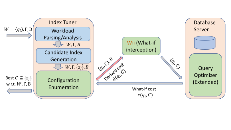
Figure 1. The architecture of budget-aware index tuning with “Wii”, i.e., what-if (call) interception, where $W$ represents the input workload, $q_{i}\in W$ represents an individual SQL query in the workload, $\Gamma$ represents a set of tuning constraints, $B$ represents the budget on the number of what-if calls allowed. Moreover, $\{z_{j}\}$ represents the set of candidate indexes generated for $W$, and $C\subseteq\{z_{j}\}$ represents an index configuration proposed during configuration enumeration.

A what-if call takes as input a query-configuration pair (QCP) and returns the estimated cost of the query by utilizing the indexes in the configuration. It is the same as a regular query optimizer call except for that it also takes hypothetical indexes, i.e., indexes that are proposed by the index tuner but have not been materialized, into consideration (Chaudhuri and Narasayya, 1998; Valentin et al., 2000). There can be thousands or even millions of potential what-if calls when tuning large and complex workloads (Siddiqui and Wu, 2023). Therefore, it is not feasible to make a what-if call for every QCP encountered in configuration enumeration/search. As a result, one key problem in budget-aware index tuning is budget allocation, where one needs to determine which QCP’s to make what-if calls for so that the index tuner can find the best index configuration. Unfortunately, optimal budget allocation is NP-hard (Comer, 1978; Chaudhuri et al., 2004; Wu et al., 2022). Existing budget-aware configuration search algorithms (Wu et al., 2022) range from adaptations of the classic greedy search algorithm (Chaudhuri and Narasayya, 1997) to more sophisticated approaches with Monte Carlo tree search (MCTS) (Kocsis and Szepesvári, 2006), which allocate budget by leveraging various heuristics. For example, the greedy-search variants adopt a simple “first come first serve” (FCFS) strategy where what-if calls are allocated on demand, and the MCTS-based approach considers the rewards observed in previous budget allocation steps to decide the next allocation step. These budget allocation strategies can be inferior. In particular, we find in practice that many of the what-if calls made are unnecessary, as their corresponding what-if costs are close to the approximations given by a well-known technique called cost derivation (Chaudhuri and Narasayya, 1997). Compared to making a what-if call, cost derivation is computationally much more efficient and has been integrated into commercial index tuning software such as DTA (Chaudhuri and Narasayya, 2020; dta, 2023). In the rest of this paper, we refer to the approximation given by cost derivation as the derived cost. Figure 2 presents the distribution of the relative gap between what-if cost and derived cost when tuning the TPC-DS benchmark workload with 99 complex queries. We observe that 80% to 90% of the what-if calls were made for QCP’s with relative gap below 5%, for two state-of-the-art budget-aware configuration search algorithms two-phase greedy and MCTS (Section 2.2). If we know that the derived cost is indeed a good approximation, we can avoid such a spurious what-if call. The challenge, however, is that we need to learn this fact before the what-if call is made.

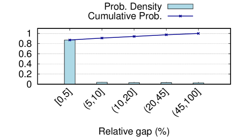
(a) two-phase greedy

(b) MCTS

Figure 2. Distribution of the relative gap between what-if cost and derived cost when tuning TPC-DS under a budget of 5,000 what-if calls. Here the relative gap is defined as $\frac{\text{derived cost}-\text{what-if cost}}{\text{derived cost}}\times 100\%$, as derived cost is an upper bound of the what-if cost under monotonicity assumption.

The best knowledge we have so far is that, under mild assumption on the monotonicity of query optimizer’s cost function (i.e., a larger configuration with more indexes should not increase the query execution cost), the derived cost acts as an upper bound of the what-if cost (Section 2.2.2). However, the what-if cost can still lie anywhere between zero and the derived cost. In this paper, we take one step further by proposing a generic framework that develops a lower bound for the what-if cost. The gap between the lower bound and the upper bound (i.e., the derived cost) therefore measures the closeness between the what-if cost and the derived cost. As a result, it is safe to avoid a what-if call when this gap is small and use the derived cost as a surrogate.

Albeit a natural idea, there are a couple of key requirements to make it relevant in practice. First, the lower bound needs to be nontrivial, i.e., it needs to be as close to the what-if cost as possible—an example of a trivial but perhaps useless lower bound would be always setting it to zero. Second, the lower bound needs to be computationally efficient compared to making a what-if call. Third, the lower bound needs to be integratable with existing budget-aware configuration enumeration algorithms. In this paper, we address these requirements as follows.

Nontriviality

We develop a lower bound that depends only on common properties of the cost functions used by the query optimizer, such as monotonicity and submodularity, which have been widely assumed by previous work (Gupta et al., 1997; Schnaitter et al., 2009; Choenni et al., 1993; Wu et al., 2013b; Leis et al., 2015) and independently verified in our own experiments (Wang et al., 2024). In a nutshell, it looks into the marginal cost improvement (MCI) that each individual index in the given configuration can achieve, and then establishes an upper bound on the cost improvement (and therefore a lower bound on the what-if cost) of the given configuration by summing up the upper bounds on the MCI’s of individual indexes (Section 3.1). We further propose optimization techniques to refine the lower bound for budget-aware greedy search algorithms (Section 4.1) and MCTS-based algorithms (Section 4.2).

Efficiency

We demonstrate that the computation time of our lower bound is orders of magnitude less compared to a what-if call, though it is in general more expensive than computing the upper bound, i.e., the derived cost (Section 6.4). For example, as shown in Figure 16(b), when running the MCTS configuration enumeration algorithm on top of the TPC-DS benchmark, on average it takes 0.02 ms and 0.04 ms to compute the derived cost and our lower bound, respectively; in contrast, the average time of making a what-if call to the query optimizer is around 800 ms.

Integratability

We demonstrate that our lower bound can be seamlessly integrated with existing budget-aware index tuning algorithms (Section 5). From a software engineering perspective, the integration is non-intrusive, meaning that there is no need to change the architecture of the current cost-based index tuning software stack. As illustrated in Figure 1, we encapsulate the lower-bound computation inside a component called “Wii,” which is shorthand for “what-if (call) interception.” During configuration enumeration, Wii intercepts every what-if call made to the query optimizer, computes the lower bound of the what-if cost, and then checks the closeness between the lower bound and the derived cost (i.e., the upper bound) with a confidence-based mechanism (Section 3.3). If Wii feels confident enough, it will skip the what-if call and instead send the derived cost back to the configuration enumerator.

More importantly, we demonstrate the efficacy of Wii in terms of (1) the number of what-if calls it allows to skip (Section 6.3) and (2) the end-to-end improvement on the final index configuration found (Section 6.2). The latter is perhaps the most valuable benefit of Wii in practice, and we show that, by reallocating the saved budget to what-if calls where Wii is less confident, it can yield significant improvement on both standard industrial benchmarks and real customer workloads (Section 6.2). For example, as showcased in Figure 6(f), with 5,000 what-if calls as budget and 20 as the maximum configuration size allowed, on TPC-DS Wii improves the baseline two-phase greedy configuration enumeration algorithm by increasing the percentage improvement of the final configuration found from 50% to 65%; this is achieved by skipping around 18,000 unnecessary what-if calls, as shown in Figure 14(b).

Last but not least, while we focus on budget-aware index tuning in this paper, Wii can also be used in a special situation where one does not enforce a budget on the index tuner, namely, the tuner has unlimited budget on the number of what-if calls. This special situation may make sense if, for example, one has a relatively small workload. Wii plays a different role here. Since there is no budget constraint, Wii cannot improve the quality of the final configuration found, as the best quality can anyways be achieved by keeping on issuing what-if calls to the query optimizer. Instead, by skipping spurious what-if calls, Wii can significantly improve the overall efficiency of index tuning. For example, without a budget constraint, when tuning the standard TPC-H benchmark with 22 queries, Wii can reduce index tuning time by 4$\times$ while achieving the same quality on the best configuration found (Section 6.8).

2. Preliminaries

In this section, we present a brief overview of the budget-aware index configuration search problem.

2.1. Cost-based Index Tuning

As Figure 1 shows, cost-based index tuning consists of two stages:

• Candidate index generation. We generate a set of candidate indexes for each query in the workload based on the indexable columns (Chaudhuri and Narasayya, 1997). Indexable columns are those that appear in the selection, join, group-by, and order-by expressions of a SQL query, which are used as key columns for fast seek-based index look-ups. We then take the union of the candidate indexes from individual queries as the candidate indexes for the entire workload.

• Configuration enumeration. We search for a subset (i.e., a configuration) of the candidate indexes that can minimize the what-if cost of the workload, with respect to constraints such as the maximum number of indexes allowed or the total amount of storage taken by the index configuration.

Index tuning is time-consuming and resource-intensive, due to the large amount of what-if calls issued to the query optimizer during configuration enumeration/search. Therefore, previous work proposes putting a budget on the amount of what-if calls that can be issued during configuration search (Wu et al., 2022). We next present this budget-aware configuration search problem in more detail.

2.2. Budget-aware Configuration Search

2.2.1. Problem Statement

Given an input workload $W$ with a set of candidate indexes $I$ (Chaudhuri and Narasayya, 1997), a set of constraints $\Gamma$, and a budget $B$ on the number of what-if calls allowed during configuration enumeration, our goal is to find a configuration $C^{*}\subseteq I$ whose what-if cost $c(W,C^{*})$ is minimized under the constraints given by $\Gamma$ and $B$.

In this paper, we focus on index tuning for data analytic workloads $W$ (e.g., the TPC-H and TPC-DS benchmark workloads). Although the constraints in $\Gamma$ can be arbitrary, we focus on the cardinality constraint $K$ that specifies the maximum configuration size (i.e., the number of indexes contained by the configuration) allowed. Moreover, under a limited budget $B$, it is often impossible to know the what-if cost of every query-configuration pair (QCP) encountered during configuration enumeration. Therefore, to estimate the costs for QCP’s where what-if calls are not allocated, one has to rely on approximation of the what-if cost without invoking the query optimizer. One common approximation technique is cost derivation (Chaudhuri and Narasayya, 1997, 2020), as we discuss below.

2.2.2. Cost Derivation

Given a QCP $(q,C)$, its derived cost $d(q,C)$ is the minimum cost over all subset configurations of $C$ with known what-if costs. Formally,

Definition 0 (Derived Cost).

The derived cost of $q$ over $C$ is

(1) $$d(q,C)=\min_{S\subseteq C}c(q,S).$$

Here, $c(q,S)$ is the what-if cost of $q$ using only a subset $S$ of indexes from the configuration $C$.

We assume the following monotone property (Gupta et al., 1997; Schnaitter et al., 2009) of index configuration costs w.r.t. to an arbitrary query $q$:

Assumption 1 (Monotonicity).

Let $C_{1}$ and $C_{2}$ be two index configurations where $C_{1}\subseteq C_{2}$. Then $c(q,C_{2})\leq c(q,C_{1})$.

That is, including more indexes into a configuration does not increase the what-if cost. Our validation results using Microsoft SQL Server show that monotonicity holds with probability between 0.95 and 0.99, on a variety of benchmark and real workloads (see (Wang et al., 2024) for details). Under Assumption 1, we have

$$d(q,C)\geq c(q,C),$$

i.e., derived cost is an upper bound $U(q,C)$ of what-if cost:

$$U(q,C)=d(q,C)=\min_{S\subseteq C}c(q,S).$$

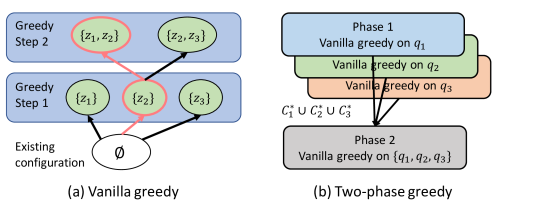
Figure 3. Example of budget-aware greedy search.

2.2.3. Existing Solutions

The budget-aware configuration search problem is NP-hard. At the core of this problem is budget allocation, namely, to decide on which QCP’s to make what-if calls. Existing heuristic solutions to the problem include: (1) vanilla greedy, (2) two-phase greedy, (3) AutoAdmin greedy, and (4) MCTS. Since (2) and (3) are similar, we omit (3) in this paper.

Vanilla greedy

Figure 3(a) illustrates the vanilla greedy algorithm with an example of three candidate indexes $\{z_{1},z_{2},z_{3}\}$ and the cardinality constraint $K=2$. Throughout this paper, we use $\emptyset$ to represent the existing configuration. Vanilla greedy works step-by-step, where each step adopts a greedy policy to choose the next index to be included that can minimize the workload cost on the chosen configuration. In this example, we have two greedy steps. The first step examines the three singleton configurations $\{z_{1}\}$, $\{z_{2}\}$, and $\{z_{3}\}$. Suppose that $\{z_{2}\}$ results in the lowest workload cost. The second step tries to expand $\{z_{2}\}$ by adding one more index, which leads to two candidate configurations $\{z_{1},z_{2}\}$ and $\{z_{2},z_{3}\}$. Suppose that $\{z_{1},z_{2}\}$ is better and therefore returned by vanilla greedy. Note that the configuration $\{z_{1},z_{3}\}$ is never visited in this example. Vanilla greedy adopts a simple “first come first serve (FCFS)” budget allocation policy to make what-if calls.

Two-phase greedy

Figure 3(b) illustrates the two-phase greedy algorithm that can be viewed as an optimization on top of vanilla greedy. Specifically, there are two phases of greedy search in two-phase greedy. In the first phase, we view each query as a workload by itself and run vanilla greedy on top of it to obtain the best configuration for that query. In this particular example, we have three queries $q_{1}$, $q_{2}$, and $q_{3}$ in the workload. After running vanilla greedy, we obtain their best configurations $C_{1}^{*}$, $C_{2}^{*}$, and $C_{3}^{*}$, respectively. In the second phase, we take the union of the best configurations found for individual queries and use that as the refined set of candidate indexes for the entire workload. We then run vanilla greedy again for the workload with this refined set of candidate indexes, as depicted in Figure 3(b) for the given example. Two-phase greedy has particular importance in practice as it has been adopted by commercial index tuning software such as Microsoft’s Database Tuning Advisor (DTA) (Chaudhuri and Narasayya, 2020; dta, 2023). Again, budget is allocated with the simple FCFS policy—the same as in vanilla greedy.

MCTS

Figure 4 illustrates the MCTS algorithm with the same example used in Figure 3. It is an iterative procedure that allocates one what-if call in each iteration until the budget runs out. The decision procedure in each iteration on which query and which configuration to issue the what-if call is an application of the classic Monte Carlo tree search (MCTS) algorithm (Browne et al., 2012) in the context of index configuration search. It involves four basic steps: (1) selection, (2) expansion, (3) simulation, and (4) update. Due to space limitation, we refer the readers to (Wu et al., 2022) for the full details of this procedure. After all what-if calls are issued, we run vanilla greedy again without making extra what-if calls to find the best configuration. Our particular version of MCTS here employs an $\epsilon$-greedy policy (Sutton and Barto, 2018) when selecting the next index to explore.

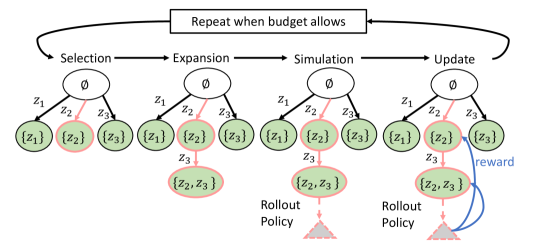
Figure 4. Example of budget allocation in MCTS.

3. What-If Call Interception

We develop “Wii” that can skip spurious what-if calls where their what-if costs and derived costs are close. One key idea is to develop a lower bound for the what-if cost: if the gap between the lower bound and the derived cost is small, then it is safe to skip the what-if call. In this section, we present the generic form of the lower bound, as well as a confidence-based framework used by Wii on top of the lower bound to skip spurious what-if calls. We defer the discussion on further optimizations of the lower bound to Section 4.

3.1. Lower Bound of What-if Cost

We use $L(q,C)$ to denote the lower bound of the what-if cost $c(q,C)$. In the following, we first introduce the notion of marginal cost improvement (MCI) of an index, which indicates the additional benefit of adding this index to a configuration for a query. We then establish $L(q,C)$ by leveraging the upper bounds of MCI.

Definition 0 (Marginal Cost Improvement).

We define the marginal cost improvement (MCI) of an index $z$ with respect to a query $q$ and a configuration $X$ as

(2) $$\delta(q,z,X)=c(q,X)-c(q,X\cup\{z\}).$$

Definition 0 (Cost Improvement).

We define the cost improvement (CI) of a query $q$ given a configuration $X$ as

(3) $$\Delta(q,X)=c(q,\emptyset)-c(q,X).$$

We can express CI in terms of MCI. Specifically, consider a query $q$ and a configuration $C=\{z_{1},...,z_{m}\}$. The cost improvement $\Delta(q,C)$ can be seen as the sum of MCI’s by adding the indexes from $C$ one by one, namely,

$$\Delta(q,C)=\Big{(}c(q,\emptyset)-c(q,\{z_{1}\})\Big{)}+\Big{(}c(q,\{z_{1}\})-c(q,\{z_{1},z_{2}\})\Big{)}$$

$$+\cdots+\Big{(}c(q,\{z_{1},...,z_{m-1}\})-c(q,C)\Big{)}.$$

Let $C_{0}=\emptyset$ and $C_{j}=C_{j-1}\cup\{z_{j}\}$ for $1\leq j\leq m$. It follows that $C_{m}=C$ and therefore, $\Delta(q,C)=\sum\nolimits_{j=1}^{m}\delta(q,z_{j},C_{j-1}).$

If we can have a configuration-independent upper bound $u(q,z_{j})$ for $\delta(q,z_{j},C_{j-1})$, namely, $u(q,z_{j})\geq\delta(q,z_{j},X)$ for any $X$, then

$$\Delta(q,C)\leq\sum\nolimits_{j=1}^{m}u(q,z_{j}).$$

As a result,

$$c(q,\emptyset)-c(q,C)\leq\sum\nolimits_{j=1}^{m}u(q,z_{j}),$$

and it follows that

$$c(q,C)\geq c(q,\emptyset)-\sum\nolimits_{j=1}^{m}u(q,z_{j}).$$

We therefore can set the lower bound $L(q,C)$ as

(4) $$L(q,C)=c(q,\emptyset)-\sum\nolimits_{j=1}^{m}u(q,z_{j}).$$

Generalization

This idea can be further generalized if we know the what-if costs of configurations that are subsets of $C$. Specifically, let $S\subset C$ be a subset of $C$ with known what-if cost $c(q,S)$. Without loss of generality, let $C-S=\{z_{1},...,z_{k}\}$. We have

$$c(q,S)-c(q,C)=\sum\nolimits_{i=1}^{k}\Big{(}c(q,C_{i-1})-c(q,C_{i})\Big{)}\leq\sum\nolimits_{i=1}^{k}u(q,z_{i}),$$

where $C_{0}$ is now set to $S$. Therefore,

$$c(q,C)\geq c(q,S)-\sum\nolimits_{i=1}^{k}u(q,z_{i}).$$

Since $S$ is arbitrary, we conclude

$$c(q,C)\geq\max_{S\subset C}\Big{(}c(q,S)-\sum\nolimits_{z\in C-S}u(q,z)\Big{)}.$$

As a result, it is safe to set

(5) $$L(q,C)=\max_{S\subset C}\Big{(}c(q,S)-\sum\nolimits_{z\in C-S}u(q,z)\Big{)}.$$

Since $\emptyset\subset C$, Equation 5 is a generalization of Equation 4.

3.2. Upper Bound of MCI

The main question is then to maintain an upper bound $u(q,z)$ for the MCI of each query $q$ and each individual index $z$ so that $u(q,z)\geq\delta(q,z,X)$ for any configuration $X$. Below we discuss several such upper bounds. Our basic idea is to leverage the CIs of explored configurations that contain $z$, along with some well-known properties, such as monotonicity and submodularity, of the cost function used by the query optimizer.

3.2.1. Naive Upper Bound

Let $\Omega$ be the set of all candidate indexes.

Definition 0 (Naive Upper Bound).

Under Assumption 1,

(6) $$u(q,z)=c(q,\emptyset)-c(q,\Omega)=\Delta(q,\Omega)$$

is a valid upper bound of $\delta(q,z,X)$ for any $X$.

Intuitively, by the monotonicity property, the MCI of any single index $z$ cannot be larger than the CI of all candidate indexes in $\Omega$ combined. In practical index tuning applications, we often have $c(q,\Omega)$ available. However, if $c(q,\Omega)$ is unavailable, then we set $u(q,z)=c(q,\emptyset)$ as it always holds that $c(q,\Omega)\geq 0$.

3.2.2. Upper Bound by Submodularity

We can improve over the naive upper bound by assuming that the cost function is submodular, which has been studied by previous work (Choenni et al., 1993).

Assumption 2 (Submodularity).

Given two configurations $X\subseteq Y$ and an index $z\not\in Y$, we have

(7) $$c(q,Y)-c(q,Y\cup\{z\})\leq c(q,X)-c(q,X\cup\{z\}).$$

Or equivalently, $\delta(q,z,Y)\leq\delta(q,z,X)$.

That is, the MCI of an index $z$ diminishes when $z$ is included into larger configuration with more indexes. Submodularity does not hold often due to index interaction (Schnaitter et al., 2009). We also validated the submodularity assumption using Microsoft SQL Server and the same workloads that we used to validate the monotonicity assumption. Our validation results show that submodularity holds with probability between 0.75 and 0.89 on the workloads tested (Wang et al., 2024).

Lemma 0.

Under Assumption 2, we have

$$\delta(q,z,X)\leq\Delta(q,\{z\})$$

for any configuration $X$.

Due to space constraint, all proofs are postponed to the full version of this paper (Wang et al., 2024). Intuitively, Lemma 4 indicates that the CI of a singleton configuration $\{z\}$ can be used as an upper bound of the MCI of the index $z$. As a result, we can set

(8) $$u(q,z)=\Delta(q,\{z\})=c(q,\emptyset)-c(q,\{z\}).$$

There are cases where $c(q,\{z\})$ is unknown but we know the cost of some configuration $X$ that contains $z$, e.g., in MCTS where configurations are explored in random order. By Assumption 1,

$$c(q,\{z\})\geq\max_{z\in X}c(q,X).$$

Therefore, we can generalize Equation 8 to have

Definition 0 (Submodular Upper Bound).

$$u(q,z) = c(q,\emptyset)-\max_{z\in X}c(q,X)$$

$$= \min_{z\in X}\Big{(}c(q,\emptyset)-c(q,X)\Big{)}$$

$$= \min_{z\in X}\Delta(q,X).$$

That is, the MCI of an index should be no larger than the minimum CI of all the configurations that contain it.

3.2.3. Summary

To summarize, assuming monotonicity and submodularity of the cost function $c$, we can set $u(q,z)$ as follows:

(9) $$u(q,z)=\min\{c(q,\emptyset),\Delta(q,\Omega),\Delta(q,\{z\}),\min_{z\in X}\Delta(q,X)\}.$$

3.3. Confidence-based What-if Call Skipping

Intuitively, the confidence of skipping the what-if call for a QCP $(q,C)$ depends on the closeness between the lower bound $L(q,C)$ and the upper bound $U(q,C)$, i.e., the derived cost $d(q,C)$. We define the gap between $U(q,C)$ and $L(q,C)$ as

$$G(q,C)=U(q,C)-L(q,C).$$

Clearly, the larger the gap is, the lower the confidence is. Therefore, it is natural to define the confidence as

(10) $$\alpha(q,C)=1-\frac{G(q,C)}{U(q,C)}=\frac{L(q,C)}{U(q,C)}.$$

Following this definition, we have $0\leq\alpha(q,C)\leq 1$. We further note two special cases: (1) $\alpha(q,C)=0$, which implies $L(q,C)=0$; and (2) $\alpha(q,C)=1$, which implies $L(q,C)=U(q,C)$.

Let $\alpha\in[0,1]$ be a threshold for the confidence, i.e., it is the minimum confidence for skipping a what-if call and we require $\alpha(q,C)\geq\alpha$. Intuitively, the higher $\alpha$ is, the higher confidence that a what-if call can be skipped with. In our experimental evaluation, we further varied $\alpha$ to test the effectiveness of this confidence-based interception mechanism (see Section 6).

4. Optimization

We present two optimization techniques for the generic lower bound detailed in Section 3.1, which is agnostic to budget-aware configuration enumeration algorithms—it only relies on general assumptions (i.e., monotonicity and submodularity) of the cost function $c$. One optimization is dedicated to budget-aware greedy search (i.e., vanilla/two-phase greedy), which is of practical importance due to its adoption in commercial index tuning software (Chaudhuri and Narasayya, 2020) (Section 4.1). The other optimization is more general and can also be used for other configuration enumeration algorithms mentioned in Section 2.2.3 such as MCTS (Section 4.2).

4.1. MCI Upper Bounds for Greedy Search

We propose the following optimization procedure for maintaining the MCI upper-bound $u(q,z)$, which is the basic building block of the lower bound presented in Section 3.1, in vanilla greedy and two-phase greedy (see Section 2):

Procedure 1.

For each index $z$ that has not been selected by greedy search, we can update $u(q,z)$ w.r.t. the current configuration selected by greedy search as follows:

1. Initialize $u(q,z)=\min\{c(q,\emptyset),\Delta(q,\Omega)\}$ for each index $z$.

2. During each greedy step $1\leq k\leq K$, update

   $$u(q,z)=c(q,C_{k-1})-c(q,C_{k-1}\cup\{z\})=\delta(q,z,C_{k-1})$$

   if both $c(q,C_{k-1})$ and $c(q,C_{k-1}\cup\{z\})$ are available.

In step (2), $C_{k}$ is the configuration selected by greedy search in step $k$ and we set $C_{0}=\emptyset$. A special case is when $k=1$, if we know $c(q,\{z\})$ then we can update $u(q,z)=c(q,\emptyset)-c(q,\{z\})=\Delta(q,\{z\})$, which reduces to the general upper bound (see Lemma 4).

Theorem 1.

Under Assumptions 1 and 2, Procedure 1 is correct, i.e., the $u(q,z)$ after each update remains an MCI upper bound w.r.t. any future configuration $X$ explored by greedy search.

4.2. Coverage-based Refinement

The tightness of the MCI upper bounds in Section 3.2 largely depends on the knowledge about $c(q,\{z\})$, namely, what-if costs of singleton configurations with one single index. Unfortunately, such information is often unavailable, and the MCI upper bound in Equation 9 is reduced to its naive version (Equation 6). For vanilla greedy and two-phase greedy, this implies that none of the QCP’s with singleton configurations can be skipped under a reasonable confidence threshold (e.g., 0.8), which can take a large fraction of the budget, although the bounds are effective at skipping what-if calls for multi-index configurations; for MCTS where configurations are explored in a random order, this further implies that skipping can be less effective for multi-index configurations as they are more likely to contain indexes with unknown what-if costs, in contrast to greedy search where multi-index configurations are always explored after singleton configurations. To overcome this limitation, we propose refinement techniques based on estimating the what-if cost $c(q,\{z\})$ if it is unknown, by introducing the notion of “coverage.”

4.2.1. Definition of Coverage

We assume that $c(q,\Omega)$ is known for each query $q$. Moreover, we assume that we know the subset $\Omega_{q}\subset\Omega$ of indexes that appear in the optimal plan of $q$ by using indexes in $\Omega$. Clearly, $c(q,\Omega)=c(q,\Omega_{q})$.

For an index $z$, we define its coverage on the query $q$ as

(11) $$\rho(q,z)=\frac{c(q,\emptyset)-c(q,\{z\})}{c(q,\emptyset)-c(q,\Omega_{q})}=\frac{\Delta(q,\{z\})}{\Delta(q,\Omega_{q})}.$$

In other words, coverage measures the relative cost improvement of $z$ w.r.t. the maximum possible cost improvement over $q$ delivered by $\Omega_{q}$. If we know $\rho(q,z)$, the cost $c(q,\{z\})$ can be recovered as

$$c(q,\{z\}) = c(q,\emptyset)-\rho(q,z)\cdot\Big{(}c(q,\emptyset)-c(q,\Omega_{q})\Big{)}$$

$$= \Big{(}1-\rho(q,z)\Big{)}\cdot c(q,\emptyset)+\rho(q,z)\cdot c(q,\Omega_{q}).$$

In the following, we present techniques to estimate $\rho(q,z)$ based on the similarities between index configurations, in particular $\{z\}$ and $\Omega_{q}$.

4.2.2. Estimation of Coverage

We estimate coverage based on the assumption that it depends on the similarity between $\{z\}$ and $\Omega_{q}$. Specifically, let $\operatorname{Sim}(\{z\},\Omega_{q})$ be some similarity measure that is between 0 and 1, and we define

$$\rho(q,z)=\operatorname{Sim}(\{z\},\Omega_{q}).$$

The problem is then reduced to developing an appropriate similarity measure. Our current solution is the following, while further improvement is possible and left for future work.

Configuration Representation

We use a representation similar to the one described in DBA bandits (Perera et al., 2021) that converts an index $z$ into a feature vector $\vec{\mathbf{z}}$. Specifically, we use one-hot encoding based on all indexable columns identified in the given workload $W$. Let $\mathcal{D}=\{c_{1},...,c_{L}\}$ be the entire domain of these $L$ indexable columns. For a given index $z$, $\vec{\mathbf{z}}$ is an $L$-dimensional vector. If some column $c_{l}\in\mathcal{D}$ ($1\leq l\leq L$) appears in $z$, then $\vec{\mathbf{z}}[l]$ receives some nonzero weight $w_{l}$ based on the weighing policy described below:

• If $c_{l}$ is the $j$-th key column of $z$, $w_{l}=\frac{1}{2^{j-1}}$;

• If $c_{l}$ is an included column of $z$, $w_{l}=\frac{1}{2^{J}}$ where $J$ is the number of key columns contained by $z$.

Otherwise, we set $\vec{\mathbf{z}}[l]=0$. Note that the above weighing policy considers the columns contained by an index as well as their order. Intuitively, leading columns in index keys play a more important role than other columns (e.g., for a “range predicate”, an access path chosen by the query optimizer needs to match the “sort order” specified in the index key columns).

We further combine feature vectors of individual indexes to generate a feature vector for the entire configuration. Specifically, consider a configuration $C=\{z_{1},...,z_{m}\}$ and let $\vec{\mathbf{z}}_{i}$ be the feature representation of the index $z_{i}$ ($1\leq i\leq m$). The feature representation $\vec{\mathbf{C}}$ of $C$ is again an $L$-dimensional vector where

$$\vec{\mathbf{C}}[l]=\max\{\vec{\mathbf{z}}_{1}[l],...,\vec{\mathbf{z}}_{m}[l]\},\text{ for }1\leq l\leq L.$$

That is, the weight $\vec{\mathbf{C}}[l]$ is the largest weight of the $l$-th dimension among the indexes contained by $C$. In particular, we generate the feature vector $\vec{\mathbf{\Omega}}_{q}$ for $\Omega_{q}$ in this way.

Query Representation

We further use a representation similar to the one described in ISUM (Siddiqui et al., 2022a) to represent a query $q$ as a feature vector $\vec{\mathbf{q}}$. Specifically, we again use one-hot encoding for the query $q$ with the same domain $\mathcal{D}=\{c_{1},...,c_{L}\}$ of all indexable columns. If some column $c_{l}\in\mathcal{D}$ appears in the query $q$, we assign a nonzero weight to $\vec{\mathbf{q}}[l]$; otherwise, $\vec{\mathbf{q}}[l]=0$. Here, we use the same weighing mechanism as used by ISUM. That is, the weight of a column is computed based on its corresponding table size and the number of candidate indexes that contain it. The intuition is that a column from a larger table and contained by more candidate indexes is more important and thus is assigned a higher weight.

Similarity Measure

Before measuring the similarity, we first project $\vec{\mathbf{z}}$ and $\vec{\mathbf{\Omega}}_{q}$ onto $\vec{\mathbf{q}}$ to get their images under the context of the query $q$. The projection is done by taking the element-wise dot product, i.e., $\tilde{\mathbf{z}}=\vec{\mathbf{z}}\cdot\vec{\mathbf{q}}$ and $\tilde{\mathbf{\Omega}}_{q}=\vec{\mathbf{\Omega}}_{q}\cdot\vec{\mathbf{q}}$. Note that $\tilde{\mathbf{z}}$ and $\tilde{\mathbf{\Omega}}_{q}$ remain vectors. We now define the similarity measure as

(12) $$\operatorname{Sim}(\{z\},\Omega_{q})=\frac{\langle\tilde{\mathbf{z}},\tilde{\mathbf{\Omega}}_{q}\rangle}{|\tilde{\mathbf{\Omega}}_{q}|^{2}}=\frac{|\tilde{\mathbf{z}}|\cdot|\tilde{\mathbf{\Omega}}_{q}|\cdot\cos\theta}{|\tilde{\mathbf{\Omega}}_{q}|^{2}}=\frac{|\tilde{\mathbf{z}}|\cdot\cos\theta}{|\tilde{\mathbf{\Omega}}_{q}|},$$

where $\theta$ represents the angle between the two vectors $\tilde{\mathbf{z}}$ and $\tilde{\mathbf{\Omega}}_{q}$.

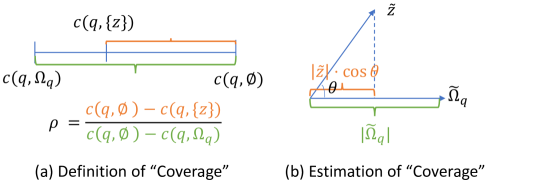
Figure 5. The definition and estimation of “coverage.”

Figure 5 illustrates and contrasts the definition and estimation of coverage. Figure 5(a) highlights the observation that $c(q,\{z\})$ must lie between $c(q,\Omega_{q})$ and $c(q,\emptyset)$, and coverage measures the cost improvement $\Delta(q,\Omega_{q})$ of $\Omega_{q}$ (i.e., the green segment) that is covered by the cost improvement $\Delta(q,\{z\})$ of $\{z\}$ (i.e., the orange segment). On the other hand, Figure 5(b) depicts the geometric view involved in the estimation of coverage using the similarity metric $\operatorname{Sim}(\{z\},\Omega_{q})$. Intuitively, the similarity measures how much “length” of the configuration $\Omega_{q}$ is covered by the “length” of the index $z$ when projected to the (same) “direction” of $\Omega_{q}$ in the feature vector space. Note that it is not important whether the lengths are close to the corresponding cost improvements—only their ratio matters. Based on our evaluation, the estimated coverage using Equation 12 is close to the ground-truth coverage in Equation 11 (see the full version of this paper (Wang et al., 2024) for details).

5. Integration

In this section, we present design considerations and implementation details when integrating Wii with existing budget-aware configuration search algorithms. We start by presenting the API functions provided by Wii. We then illustrate how existing budget-aware configuration enumeration algorithms can leverage the Wii API’s without modification to the algorithms.

5.1. Wii API Functions

As illustrated in Figure 1, Wii sits between the index tuner and the query optimizer. It offers two API functions that can be invoked by a budget-aware configuration enumeration algorithm: (1) InitMCIBounds that initializes the MCI upper-bounds $u(q,z)$; and (2) EvalCost that obtains the cost of a QCP $(q,C)$ in a budget-aware manner by utilizing the lower bound $L(q,C)$ and the upper bound $U(q,C)$, i.e., the derived cost $d(q,C)$.

Input: $W$, the workload; $I$, the candidate indexes.

Output: $u$, the initialized MCI upper bounds.

1 foreach $q\in W$ do

2    $I_{q}\leftarrow$GetCandidateIndexes($q$, $I$);

3    foreach $z\in I_{q}$ do

4       if $c(q,\Omega_{q})$ is available then

5          $u(q,z)\leftarrow c(q,\emptyset)-c(q,\Omega_{q})$;

6         

7      else

8          $u(q,z)\leftarrow c(q,\emptyset)$;

9         

Algorithm 1 InitMCIBounds($W$, $I$)

5.1.1. The InitMCIBounds Function

Algorithm 1 presents the details. It initializes the MCI upper bound $u(q,z)$ for each query $q\in W$ and each of its candidate indexes $z\in I_{q}$. If $c(q,\Omega_{q})$ is available, it uses the naive upper bound (Equation 6); otherwise, it uses $c(q,\emptyset)$.

5.1.2. The EvalCost Function

Algorithm 2 presents the details. If the what-if cost $c(q,C)$ is known, it simply uses that and updates the MCI upper-bounds (lines 1 to 3). Otherwise, it checks whether the budget $B$ on the number of what-if calls has been reached and returns the derived cost $d(q,C)$ if so (lines 4 to 5). On the other hand, if there is remaining budget, i.e., $B>0$, it then tries to use the upper-bound $U(q,C)$ and the lower-bound $L(q,C)$ to see whether the what-if call for $(q,C)$ can be skipped; if so, the derived cost $d(q,C)$ is returned (lines 6 to 11)—the budget $B$ remains the same in this case. Finally, if the confidence of skipping is low, we make one what-if call to obtain $c(q,C)$ (lines 12 to 13) and update the MCI upper-bounds (line 14). As a result, we deduct one from the current budget $B$ (line 15).

Input: $q$, the query; $C$, the configuration; $B$, the budget on the number of what-if calls; $\alpha$, the threshold on the confidence $\alpha(q,C)$; $S$, an (optional) subset of $C$ with known what-if cost $c(q,S)$, which defaults to the existing configuration $\emptyset$.

Output: $\operatorname{cost}(q,C)$, the cost of $q$ w.r.t. $C$; $B^{\prime}$, the remaining budget.

1 if $c(q,C)$ is known then

2    UpdateMCIBounds($C$, $S$);

3    return ($\operatorname{cost}(q,C)\leftarrow c(q,C)$, $B^{\prime}\leftarrow B$);

4   

5 if $B$ is zero then

6    return ($\operatorname{cost}(q,C)\leftarrow d(q,C)$, $B^{\prime}\leftarrow 0$);

7   

8 ## $c(q,C)$ is unknown and we still have budget.

9 $U(q,C)\leftarrow d(q,C)$;

10 $L(q,C)\leftarrow\max\{0,c(q,\Omega_{q}),c(q,S)-\sum_{x\in C-S}u(q,x)\}$;

11 if $\alpha(q,C)=\frac{L(q,C)}{U(q,C)}\geq\alpha$ then

12    ## The confidence is high enough.

13    return ($\operatorname{cost}(q,C)\leftarrow d(q,C)$, $B^{\prime}\leftarrow B$);

14   

15## Need to go to the query optimizer to get $c(q,C)$.

16 $c(q,C)\leftarrow$WhatIfCall($q$, $C$);

17 UpdateMCIBounds($C$, $S$);

18 return ($\operatorname{cost}(q,C)\leftarrow c(q,C)$, $B^{\prime}\leftarrow B-1$);

19 

20 UpdateMCIBounds($C$, $S$)

21 ## Update the MCI bounds based on $c(q,C)$ and $c(q,S)$.

22 foreach $x\in C-S$ do

23    $u(q,x)\leftarrow\min\{u(q,x),c(q,S)-c(q,C)\}$;

24   

Algorithm 2 EvalCost($q$, $C$, $B$, $\alpha$, $S\leftarrow\emptyset$)

One may have noticed the optional input parameter $S$ in Algorithm 2, which represents some subset configuration of $C$ and is set to be the existing configuration $\emptyset$ by default. We will discuss how to specify this parameter when using Wii in existing budget-aware configuration enumeration algorithms (e.g., greedy search and MCTS) shortly.

5.2. Budget-aware Greedy Search

To demonstrate how to use the Wii API’s without modifying the existing budget-aware configuration search algorithms, Algorithm 3 showcases how these API’s can be used by budget-aware greedy search, a basic building block of the existing algorithms. Notice that the InitMCIBounds API is invoked at line 1, whereas the EvalCost API is invoked at line 9, which are the only two differences compared to regular budget-aware greedy search. Therefore, there is no intrusive change to the greedy search procedure itself.

Remarks

We have two remarks here. First, when calling Wii to evaluate cost at line 9, we pass $C^{*}$ to the optional parameter $S$ in Algorithm 2. Note that this is just a special case of Equation 5 for greedy search, as stated by the following theorem:

Theorem 1.

In the context of greedy search, Equation 5 reduces to

$$L(q,C_{z})=c(q,C^{*})-\sum\nolimits_{x\in C_{z}-C^{*}}u(q,x)=c(q,C^{*})-u(q,z),$$

where $C_{z}=C^{*}\cup\{z\}$ and $C^{*}$ is the latest configuration selected by budget-aware greedy search (as shown in Algorithm 3).

Second, in the context of greedy search, the update step at line 20 of Algorithm 2 becomes

$$u(q,x)\leftarrow\min\{u(q,x),c(q,C^{*})-c(q,C)\}.$$

The correctness of this update has been given by Theorem 1.

Input: $W$, the workload; $I$, the candidate indexes; $K$, the cardinality constraint; $B$, the budget on the number of what-if calls; $\alpha$, the confidence threshold.

Output: $C^{*}$, the best configuration; $B^{\prime}$, the remaining budget.

1 InitMCIBounds($W$, $I$);

2 $C^{*}\leftarrow\emptyset$, $\operatorname{cost}^{*}\leftarrow\operatorname{cost}(W,\emptyset)$, $B^{\prime}\leftarrow B$;

3 while $I\neq\emptyset$ and $|C^{*}|<K$ do

4    $C\leftarrow C^{*}$, $\operatorname{cost}\leftarrow\operatorname{cost}^{*}$;

5    foreach index $z\in I$ do

6       $C_{z}\leftarrow C^{*}\cup\{z\}$;

7       $\operatorname{cost}(W,C_{z})\leftarrow 0$;

8       foreach $q\in W$ do

9          $\Big{(}\operatorname{cost}(q,C_{z}),B^{\prime}\Big{)}\leftarrow$EvalCost$(q,C_{z},B^{\prime},\alpha,C^{*})$;

10          $\operatorname{cost}(W,C_{z})\leftarrow\operatorname{cost}(W,C_{z})+\operatorname{cost}(q,C_{z})$;

11         

12      if $\operatorname{cost}(W,C_{z})<\operatorname{cost}$ then

13          $C\leftarrow C_{z}$, $\operatorname{cost}\leftarrow\operatorname{cost}(W,C_{z})$;

14         

15      

16   if $\operatorname{cost}\geq\operatorname{cost}^{*}$ then

17       return ($C^{*}$, $B^{\prime}$);

18      

19   else

20       $C^{*}\leftarrow C$, $\operatorname{cost}^{*}\leftarrow\operatorname{cost}$, $I\leftarrow I-C^{*}$;

21      

22   

23return ($C^{*}$, $B^{\prime}$);

Algorithm 3 GreedySearch($W$, $I$, $K$, $B$, $\alpha$)

5.3. Budget-aware Configuration Enumeration

We now outline the skeleton of existing budget-aware configuration enumeration algorithms after integrating Wii. We use the integrated budget-aware greedy search procedure in Algorithm 3 as a building block in our illustration.

5.3.1. Vanilla Greedy

The vanilla greedy algorithm after integrating Wii is exactly the same as the GreedySearch procedure presented by Algorithm 3.

5.3.2. Two-phase Greedy

Algorithm 4 presents the details of the two-phase greedy algorithm after integrating Wii. There is no change to two-phase greedy except for using the version of GreedySearch in Algorithm 3. The function GetCandidateIndexes selects a subset of candidate indexes $I_{q}$ from $I$, considering only the indexable columns contained by the query $q$ (Chaudhuri and Narasayya, 1997).

Input: $W$, the workload; $I$, the candidate indexes; $K$, the cardinality constraint; $B$, the budget on the number of what-if calls; $\alpha$, the confidence threshold.

Output: $C^{*}$, the best configuration; $B^{\prime}$, the remaining budget.

1 $I_{W}\leftarrow\emptyset$, $B^{\prime}\leftarrow B$;

2 foreach $q\in W$ do

3    $I_{q}\leftarrow$GetCandidateIndexes($q$, $I$);

4    $\Big{(}C_{q},B^{\prime}\Big{)}\leftarrow$GreedySearch($\{q\}$, $I_{q}$, $K$, $B^{\prime}$, $\alpha$);

5    $I_{W}\leftarrow I_{W}\cup C_{q}$;

6   

7$\Big{(}C^{*},B^{\prime}\Big{)}\leftarrow$GreedySearch($W$, $I_{W}$, $K$, $B^{\prime}$, $\alpha$);

8 return $\Big{(}C^{*},B^{\prime}\Big{)}$;

Algorithm 4 TwoPhaseGreedy($W$, $I$, $K$, $B$, $\alpha$)

5.3.3. MCTS

Algorithm 5 presents the skeleton of MCTS after Wii is integrated. The details of the three functions InitMCTS, SelectQueryConfigByMCTS, and UpdateRewardForMCTS can be found in (Wu et al., 2022). Again, there is no change to the MCTS algorithm except for that cost evaluation at line 5 is delegated to the EvalCost API of Wii (Algorithm 2).

Note that here we pass the existing configuration $\emptyset$ to the optional parameter $S$ in Algorithm 2, which makes line 8 of Algorithm 2 on computing $L(q,C)$ become

$$L(q,C)\leftarrow\max\{0,c(q,\Omega_{q}),c(q,\emptyset)-\sum\nolimits_{x\in C}u(q,x)\}.$$

Essentially, this means that we use Equation 4 for $L(q,C)$, instead of its generalized version shown in Equation 5. Although we could have used Equation 5, it was our design decision to stay with Equation 4, not only for simplicity but also because of the inefficacy of Equation 5 in the context of MCTS. This is due to the fact that in MCTS configurations and queries are explored in random order. Therefore, the subsets $S$ w.r.t. a given pair of $q$ and $C$ with known what-if costs $c(q,S)$ are sparse. As a result, Equation 5 often reduces to Equation 4 when running Wii underlying MCTS.

Input: $W$, the workload; $I$, the candidate indexes; $K$, the cardinality constraint; $B$, the budget on the number of what-if calls; $\alpha$, the confidence threshold.

Output: $C^{*}$, the best configuration; $B^{\prime}$, the remaining budget.

1 $B^{\prime}\leftarrow B$;

2 InitMCTS($W$, $I$);

3 while $B^{\prime}>0$ do

4    $(q,C)\leftarrow$SelectQueryConfigByMCTS($W$, $I$, $K$);

5    $\Big{(}\operatorname{cost}(q,C),B^{\prime}\Big{)}\leftarrow$EvalCost$(q,C,B^{\prime},\alpha,\emptyset)$;

6    UpdateRewardForMCTS($q$, $C$, $\operatorname{cost}(q,C)$);

7   

8$\Big{(}C^{*},B^{\prime}\Big{)}\leftarrow$GreedySearch($W$, $I$, $K$, $B^{\prime}$, $\alpha$);

9 return $\Big{(}C^{*},B^{\prime}\Big{)}$;

Algorithm 5 MCTS($W$, $I$, $K$, $B$, $\tau$)

6. Experimental Evaluation

We now report experimental results on evaluating Wii when integrated with existing budget-aware configuration search algorithms. We perform all experiments using Microsoft SQL Server 2017 under Windows Server 2022, running on a workstation equipped with 2.6 GHz multi-core AMD CPUs and 256 GB main memory.

6.1. Experiment Settings

Datasets

We used standard benchmarks and real workloads in our study. Table 1 summarizes the information of the workloads. For benchmark workloads, we use both the TPC-H and TPC-DS benchmarks with scaling factor 10. We also use two real workloads, denoted by Real-D and Real-M in Table 1, which are significantly more complicated compared to the benchmark workloads, in terms of schema complexity (e.g., the number of tables), query complexity (e.g., the average number of joins and table scans contained by a query), and database/workload size. Moreover, we report the number of candidate indexes of each workload, which serves as an indicator of the size of the corresponding search space faced by an index configuration search algorithm.

Algorithms Evaluated

We focus on two state-of-the-art budget-aware configuration search algorithms described in Section 2: (1) two-phase greedy, which has been adopted by commercial index tuning software (Chaudhuri and Narasayya, 2020); and (2) MCTS, which shows better performance than two-phase greedy. We omit vanilla greedy as it is significantly inferior to two-phase greedy (Wu et al., 2022). Both two-phase greedy and MCTS use derived cost as an estimate for the what-if cost when the budget on what-if calls is exhausted. We evaluate Wii when integrated with the above configuration search algorithms.

Other Experimental Settings

In our experiments, we set the cardinality constraint $K\in\{$10, 20$\}$. Since the TPC-H workload is relatively small compared to the other workloads, we varied the budget $B$ on the number of what-if calls in $\{500,1000\}$; for the other workloads, we varied the budget $B$ in $\{500,1000,2000,5000\}$.

Name	DB Size	# Queries	# Tables	Avg. # Joins	Avg. # Scans	# Candidate Indexes
TPC-H	sf=10	22	8	2.8	3.7	168
TPC-DS	sf=10	99	24	7.7	8.8	848
Real-D	587GB	32	7,912	15.6	17	417
Real-M	26GB	317	474	20.2	21.7	4,490

Table 1. Summary of database and workload statistics.

6.2. End-to-End Improvement

The evaluation metric used in our experiments is the percentage improvement of the workload based on the final index configuration found by a search algorithm, defined as

(13) $$\eta(W,C)=\Big{(}1-\frac{c(W,C)}{c(W,\emptyset)}\Big{)}\times 100\%,$$

where $c(W,C)=\sum_{q\in W}c(q,C)$. Note that here we use the query optimizer’s what-if cost estimate $c(q,C)$ as the gold standard of query execution cost, instead of using the actual query execution time, to be in line with previous work on evaluating index configuration enumeration algorithms (Chaudhuri and Narasayya, 1997; Kossmann et al., 2020).

6.2.1. Two-phase Greedy

(a) TPC-H, $K=10$

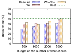
(b) TPC-DS, $K=10$

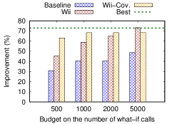
(c) Real-D, $K=10$

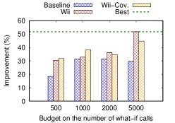
(d) Real-M, $K=10$

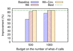
(e) TPC-H, $K=20$

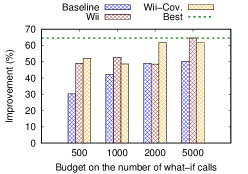
(f) TPC-DS, $K=20$

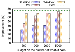
(g) Real-D, $K=20$

(h) Real-M, $K=20$

Figure 6. Results for two-phase greedy with confidence threshold $\alpha=0.9$ (“Cov.” is shorthand for “Coverage”).

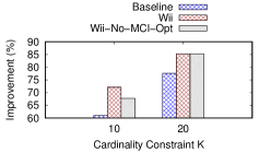
(a) TPC-H, $B=1,000$

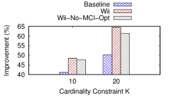
(b) TPC-DS, $B=5,000$

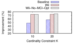
(c) Real-D, $B=5,000$

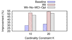
(d) Real-M, $B=5,000$

Figure 7. Impact on the performance of Wii with or without the optimization for the MCI upper bounds ($\alpha=0.9$).

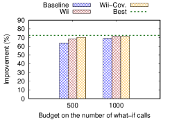
(a) TPC-H, $K=10$

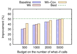
(b) TPC-DS, $K=10$

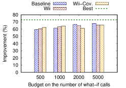
(c) Real-D, $K=10$

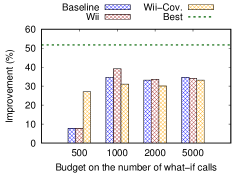
(d) Real-M, $K=10$

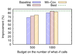
(e) TPC-H, $K=20$

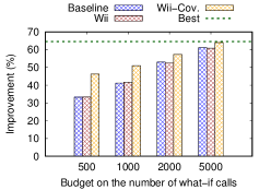
(f) TPC-DS, $K=20$

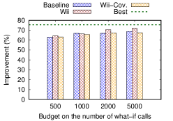
(g) Real-D, $K=20$

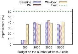
(h) Real-M, $K=20$

Figure 8. Results for MCTS with confidence threshold $\alpha=0.9$ (“Cov.” is shorthand for “Coverage”).

Figure 6 presents the evaluation results of Wii for two-phase greedy when setting the confidence threshold $\alpha=0.9$ (see Section 6.2.5 for details of the ‘Best’ lines). We observe that Wii significantly outperforms the baseline (i.e., two-phase greedy without what-if call interception). For example, when setting $K=20$ and $B=5,000$, Wii improves over the baseline by increasing the percentage improvement from 50% to 65% on TPC-DS (Figure 6(f)), from 58% to 74% on Real-D (Figure 6(g)), and from 32% to 54% on Real-M (Figure 6(h)); even for the smallest workload TPC-H, when setting $K=20$ and $B=1,000$, Wii improves over the baseline from 78% to 86% (Figure 6(e)). Note that here Wii has used the optimization for greedy search (Section 4.1).

We also observe that incorporating the coverage-based refinement described in Section 4.2 can further improve Wii in certain cases. For instance, on TPC-DS when setting $K=20$ and $B=2,000$, it improves Wii by 13%, i.e., from 49% to 62%, whereas Wii and the baseline perform similarly (Figure 6(f)); on Real-D when setting $K=10$ and $B=500$ (Figure 6(c)), it improves Wii by an additional percentage improvement of 17.8% (i.e., from 45.3% to 63.1%), which translates to 32.2% improvement over the baseline (i.e., from 30.9% to 63.1%).

Impact of Optimization for MCI Upper Bounds

We further study the impact of the optimization proposed in Section 4.1 for two-phase greedy. In our experiment, we set $\alpha=0.9$, $B=1,000$ for TPC-H and $B=5,000$ for the other workloads. Figure 7 presents the results. We observe that the optimization for MCI upper bounds offers a differentiable benefit in two-phase greedy on TPC-H, TPC-DS, and Real-M. Given its negligible computation overhead, this optimization is warranted to be enabled by default in Wii.

6.2.2. MCTS

Figure 8 presents the results of Wii for MCTS, again by setting the confidence threshold $\alpha=0.9$. Unlike the case of two-phase greedy, for MCTS Wii often performs similarly to the baseline (i.e., MCTS without what-if call interception). This is not surprising, given that MCTS already significantly outperforms two-phase greedy in many (but not all) cases, which can be verified by comparing the corresponding charts in Figure 6 and Figure 8—further improvement on top of that is more challenging. However, there are noticeable cases where we do observe significant improvement as we incorporate the coverage-based refinement into Wii. For instance, on Real-M, when setting $K=10$ and $B=500$ (Figure 8(d)), it improves over the baseline by increasing the percentage improvement of the final index configuration found by MCTS from 7.8% to 27.1%; similar observation holds when we increasing $K$ to 20 (Figure 8(h)), where we observe an even higher boost on the percentage improvement (i.e., from 8.5% to 36.9%). In general, we observe that Wii is more effective on the two larger workloads (TPC-DS and Real-M), which have more complex queries and thus much larger search spaces (ref. Table 1). In such situations, the number of configurations that MCTS can explore within the budget constraint is too small compared to the entire search space. Wii increases the opportunity for MCTS to find a better configuration by skipping spurious what-if calls. Nevertheless, compared to two-phase greedy, MCTS has its own limitations (e.g., its inherent usage of randomization) that require more research to pave its way of being adopted by commercial index tuners (Siddiqui and Wu, 2023). Moreover, MCTS is not suitable for the “unlimited budget” case (Section 6.8) as it requires a budget constraint as input.

6.2.3. Discussion

Comparing Figures 6 and 8, while the baseline version of two-phase greedy clearly underperforms that of MCTS, the Wii-enhanced version of two-phase greedy performs similarly or even better than that of MCTS. Existing budget allocation policies are largely macro-level optimization mechanisms, meaning that they deem what-if calls as atomic black-box operations that are out of their optimization scopes. However, our results here reveal that micro-level optimization mechanisms like Wii that operate at the granularity of individual what-if calls can interact with and have profound impact on the performance of those macro-level optimization mechanisms. An in-depth study and understanding of such macro-/micro-level interactions may lead to invention of better budget allocation policies.

Moreover, based on our evaluation results, the coverage-based refinement does not always improve Wii’s performance. A natural question is then how users would choose whether or not to use it. Are there some simple tests that can indicate whether or not it will be beneficial? Since the motivation of the coverage-based refinement is to make Wii work more effectively in the presence of unknown singleton-configuration what-if costs, one idea could be to measure the fraction of such singleton-configurations and enable the coverage-based refinement only when this fraction is high. However, this measurement can only be monitored “during” index tuning and there are further questions if index tuning is budget-constrained (e.g., how much budget should be allocated for monitoring this measurement). Thus, there seems to be no simple answer and we leave its investigation for future work.

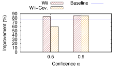
(a) TPC-H, $B=1,000$

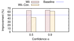
(b) TPC-DS, $B=5,000$

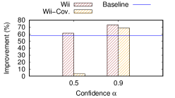
(c) Real-D, $B=5,000$

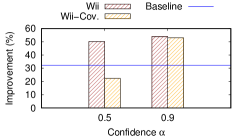
(d) Real-M, $B=5,000$

Figure 9. Performance impact when lowering the confidence threshold $\alpha$ of Wii for two-phase greedy ($K=20$).

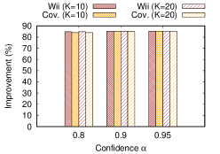
(a) TPC-H, $B=1,000$

(b) TPC-DS, $B=5,000$

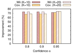
(c) Real-D, $B=5,000$

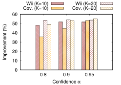
(d) Real-M, $B=5,000$

Figure 10. Impact of the confidence threshold for two-phase greedy (“Cov.” is shorthand for “Wii-Coverage”).

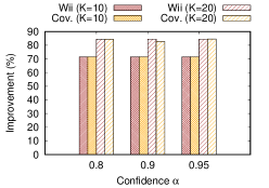
(a) TPC-H, $B=1,000$

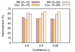
(b) TPC-DS, $B=5,000$

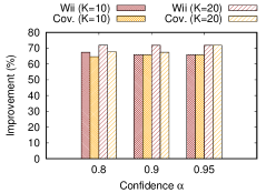
(c) Real-D, $B=5,000$

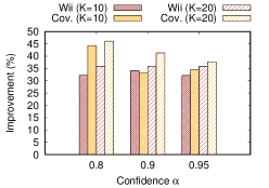
(d) Real-M, $B=5,000$

Figure 11. Impact of the confidence threshold for MCTS (“Cov.” is shorthand for “Wii-Coverage”).

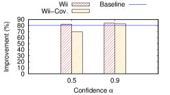
(a) TPC-H, $B=1,000$

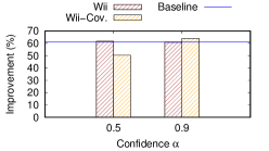
(b) TPC-DS, $B=5,000$

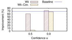
(c) Real-D, $B=5,000$

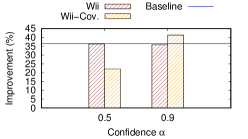
(d) Real-M, $B=5,000$

Figure 12. Performance impact when lowering the confidence threshold $\alpha$ used by Wii for MCTS ($K=20$).

6.2.4. Evaluation of Confidence-based What-if Call Skipping

We start by investigating the impact of the confidence threshold $\alpha$ on Wii. For this set of experiments, we use the budget $B=1,000$ for TPC-H and use $B=5,000$ for the other workloads, and we vary $\alpha\in\{0.8,0.9,0.95\}$. Figures 10 and 11 present the evaluation results. We observe that Wii is not sensitive to the threshold $\alpha$ within the range that we tested, for both two-phase greedy and MCTS. On the other hand, coverage-based refinement is more sensitive to $\alpha$. For instance, for two-phase greeedy on Real-M with cardinality constraint $K=10$ (ref. Figure 10(d)), the end-to-end percentage improvement of the final configuration found increases from 35.6% to 53.3% when raising $\alpha$ from 0.8 to 0.95. This suggests both opportunities and risks of using the coverage-based refinement for Wii, as one needs to choose the confidence threshold $\alpha$ more carefully. A more formal analysis can be found in (Wang et al., 2024).

Low Confidence Threshold

An interesting question is the performance impact of using a relatively lower confidence threshold compared to the ones used in the previous evaluations. To investigate this question, we further conduct experiments by setting the confidence threshold $\alpha=0.5$. Figures 9 and 12 present results for two-phase greedy and MCTS with the cardinality constraint $K=20$. We have the following observations. First, the performance of Wii often becomes much worse compared to using a high confidence threshold like the $\alpha=0.9$ in the charts—it is sometimes even worse than the baseline, e.g., in the case of MCTS on Real-D, as shown in Figure 12(c). Second, coverage-based refinement seems more sensitive to the use of a low confidence threshold, due to its inherent uncertainty of estimating singleton-configuration what-if costs.

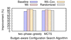
(a) TPC-H, $B=1,000$

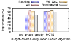
(b) TPC-DS, $B=5,000$

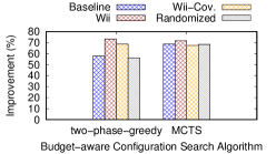
(c) Real-D, $B=5,000$

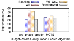
(d) Real-M, $B=5,000$

Figure 13. Confidence-based skipping vs. randomized skipping of what-if calls ($p=\alpha=0.9$, $K=20$).

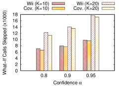
(a) TPC-H, $B=1,000$

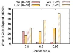
(b) TPC-DS, $B=5,000$

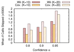
(c) Real-D, $B=5,000$

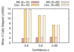
(d) Real-M, $B=5,000$

Figure 14. Amount of what-if calls skipped by Wii for two-phase greedy (“Cov.” is shorthand for “Wii-Coverage”).

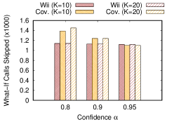
(a) TPC-H, $B=1,000$

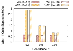
(b) TPC-DS, $B=5,000$

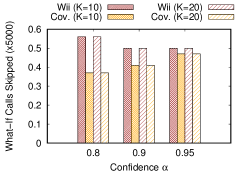
(c) Real-D, $B=5,000$

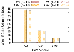
(d) Real-M, $B=5,000$

Figure 15. Amount of what-if calls skipped by Wii for MCTS (“Cov.” is shorthand for “Wii-Coverage”).

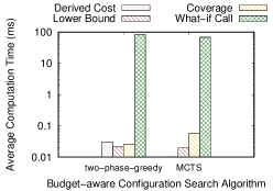
(a) TPC-H, $B=1,000$

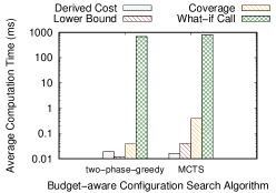
(b) TPC-DS, $B=5,000$

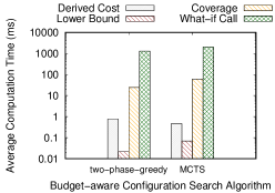
(c) Real-D, $B=5,000$

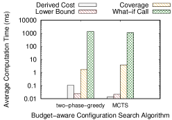
(d) Real-M, $B=5,000$

Figure 16. Average computation time (in milliseconds) of the lower bound on the what-if cost ($K=20$, $\alpha=0.9$).

Necessity of Confidence-based Mechanism

Since the confidence-based skipping mechanism comes with additional overhead of computing the lower and upper bounds of what-if cost (Section 6.4), it is natural to ask whether such complexity is necessary. To justify this, we compare the confidence-based mechanism with a simple randomized mechanism that skips what-if calls randomly w.r.t. a given skipping probability threshold $p$. Figure 13 presents the results when setting $p=\alpha=0.9$—we use the same confidence threshold for a fair comparison. We observe that the randomized mechanism performs similarly to the baseline but often much worse than Wii.

6.2.5. Best Possible Improvement

It is difficult to know the best possible improvement without making a what-if call for every QCP enumerated during configuration search, which is infeasible in practice. We provide an approximate assessment by using a much larger budget $B$ in two-phase greedy. Specifically, we use $B=5,000$ for TPC-H and $B=20,000$ for the other workloads. For each workload, we run both two-phase greedy without and with Wii, and we take the best improvement observed in these two runs. The ‘Best’ line in Figures 6 and 8 presents this result.

6.3. Efficacy of What-If Call Interception

We measure the relative amount of what-if calls skipped by Wii, namely, the ratio between the number of what-if calls skipped and the budget allowed. Figures 14 and 15 present the results for two-phase greedy and MCTS when varying $\alpha\in\{0.8,0.9,0.95\}$.

We have several observations. First, in general, Wii is more effective at skipping spurious what-if calls for two-phase greedy than MCTS. For example, when setting $K=20$ and $\alpha=0.9$, Wii is able to skip $3.6B$ (i.e., $3.6\times 5,000=18,000$) what-if calls for two-phase greedy whereas only $0.57B$ (i.e., 2,850) what-if calls for MCTS. This is correlated with the observation that Wii exhibits more significant end-to-end improvement in terms of the final index configuration found for two-phase greedy than MCTS, as we highlighted in Section 6.2. Second, the coverage-based refinement often enables Wii to skip more what-if calls. For instance, for MCTS on Real-M when setting $K=20$ and $\alpha=0.8$, Wii is able to skip only $1.48B$ (i.e., 7,400) what-if calls, which leads to no observable end-to-end improvement over the baseline; with the coverage-based refinement enabled, however, the number of what-if calls that Wii can skip rises to $42.7B$ (i.e., 213,500), which results in nearly 10% boost on the end-to-end improvement (ref. Figure 11(d)). Third, while one would expect that the amount of what-if calls skipped decreases when we increase the confidence threshold $\alpha$, this is sometimes not the case, especially for two-phase greedy. As shown in Figures 14(a), 14(b), and 14(c), the number of skipped calls can actually increase when raising $\alpha$. The reason for this unexpected phenomenon is the special structure of the two-phase greedy algorithm: lowering $\alpha$ allows for more what-if calls to be skipped in the first phase where the goal is to find good candidate indexes for each individual query. Skipping more what-if calls in the first phase therefore can result in fewer candidate indexes being selected because, without what-if calls, the derived costs for the candidate indexes will have the same value (as the what-if cost with the existing index configuration, i.e., $c(q,\emptyset)$) and thus exit early in Algorithm 3 (line 14). As a result, it eventually leads to a smaller search space for the second phase and therefore fewer opportunities for what-if call interception.

6.4. Computation Overhead

We measure the average computation time of the lower bound of the what-if cost. For comparison, we also report the average time of cost derivation as well as making a what-if call. Figure 16 summarizes the results when running two-phase greedy and MCTS with $K=20$ and $\alpha=0.9$.

We have the following observations. First, the computation time of the lower bound is similar to cost derivation, both of which are orders of magnitude less than the time of making a what-if call—the $y$-axis of Figure 16 is in logarithmic scale. Second, the coverage-based refinement increases the computation time of the lower-bound, but it remains negligible compared to a what-if call.

Table 2 further presents the additional overhead of Wii w.r.t. the baseline configuration search algorithm without Wii, measured as a percentage of the baseline execution time. We observe that Wii’s additional overhead, with or without the coverage-based refinement, is around 3% at maximum, while the typical additional overhead is less than 0.5%.

Wii (Wii-Cov.)	two-phase greedy	MCTS
TPC-H ($B=1,000$)	0.199% (0.273%)	0.064% (0.106%)
TPC-DS ($B=5,000$)	0.016% (0.345%)	0.015% (0.164%)
Real-D ($B=5,000$)	0.087% (2.354%)	0.029% (3.165%)
Real-M ($B=5,000$)	0.055% (2.861%)	0.003% (2.544%)

Table 2. Additional overhead of Wii and Wii-Coverage, measured as percentage of the execution time of the baseline configuration search algorithm ($K=20$, $\alpha=0.9$).

6.5. Storage Constraints

As mentioned earlier, one may have other constraints in practical index tuning in addition to the cardinality constraint. One common constraint is the storage constraint (SC) that limits the maximum amount of storage taken by the recommended indexes (Kossmann et al., 2020). To demonstrate the robustness of Wii w.r.t. other constraints, we evaluate its efficacy by varying the SC as well. In our evaluation, we fix $K=20$, $\alpha=0.9$, $B=1,000$ for TPC-H and $B=5,000$ for the other workloads, while varying the allowed storage size as 2$\times$ and 3$\times$ of the database (3$\times$ is the default setting of DTA (dta, 2023)).

Figures 17 and 18 present the evaluation results for two-phase greedy and MCTS. Overall, we observe similar patterns in the presence of SC. That is, Wii, with or without the coverage-based refinement, often significantly outperforms the baseline approaches, especially for two-phase greedy.

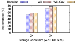
(a) TPC-H, $B=1,000$

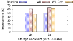
(b) TPC-DS, $B=5,000$

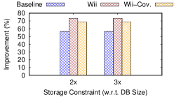
(c) Real-D, $B=5,000$

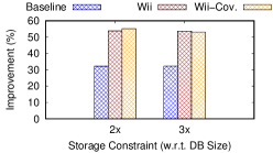
(d) Real-M, $B=5,000$

Figure 17. Evaluation results of Wii for two-phase greedy with varying storage constraints ($K=20$, $\alpha=0.9$).

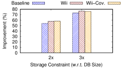
(a) TPC-H, $B=1,000$

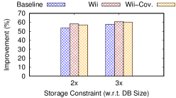
(b) TPC-DS, $B=5,000$

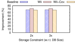
(c) Real-D, $B=5,000$

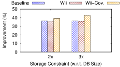
(d) Real-M, $B=5,000$

Figure 18. Evaluation results of Wii for MCTS with varying storage constraints ($K=20$, $\alpha=0.9$).

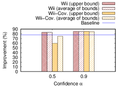
(a) TPC-H, $B=1,000$

(b) TPC-DS, $B=5,000$

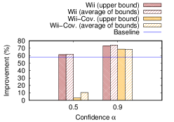
(c) Real-D, $B=5,000$

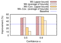
(d) Real-M, $B=5,000$

Figure 19. Using derived cost vs. the average of lower and upper bounds for two-phase greedy ($K=20$).

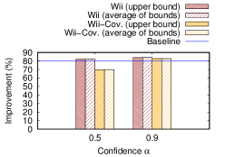
(a) TPC-H, $B=1,000$

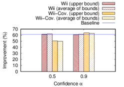
(b) TPC-DS, $B=5,000$

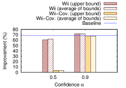
(c) Real-D, $B=5,000$

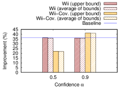
(d) Real-M, $B=5,000$

Figure 20. Using derived cost vs. the average of lower and upper bounds for MCTS ($K=20$).

6.6. Beyond Derived Cost

When Wii decides to skip a what-if call, it returns the derived cost (i.e., the upper bound) as an approximation of the what-if cost. This is not mandatory, and there are other options. For example, one can instead return the average of the lower and upper bounds. We further evaluate this idea below. Figures 19 and 20 present the results. While both options perform similarly most of the time, we observe that they perform quite differently in a few cases; moreover, one may outperform the other in these cases. For example, with the coverage-based refinement enabled in Wii, when setting $\alpha=0.5$, on TPC-H returning the average significantly outperforms returning the upper bound (74.7% vs. 59.7%); however, on Real-M returning the average loses 10.5% in percentage improvement compared to returning the upper bound (11.8% vs. 22.3%). As a result, the question of having a better cost approximation than the upper bound (i.e., the derived cost) remains open, and we leave it for future exploration.

6.7. Impact of Submodularity Assumption

Workload	Average	Median	$95^{\text{th}}$ Percentile
TPC-H	0.209	0.001	1.498
TPC-DS	2.203	0.001	10.532
Real-D	7.658	0.010	38.197
Real-M	4.125	0.001	31.358

Table 3. Magnitude of violation (of submodularity).

Although our validation results show that submodularity holds with probability between 0.75 and 0.89 on the workloads tested (Wang et al., 2024), it remains an interesting question to understand the impact on Wii when submodularity does not hold. As we mentioned in Section 3.2.2, submodularity does not hold often due to index interaction (Schnaitter et al., 2009). For example, the query optimizer may choose an index-intersection plan with two indexes available at the same time but utilizing neither if only one of them is present. In this example, submodularity does not hold, because the MCI of either index will increase after the other index is selected. As a result, Equation 8 is no longer an MCI upper-bound—it will be smaller than the actual MCI upper-bound. Consequently, the $L(q,C)$ computed by Equation 4 will be larger than the actual lower-bound of the what-if cost, which implies an overconfident situation for Wii where the confidence is computed by Equation 10. The degree of overconfidence depends on the magnitude of violation of the submodularity assumption, which we further measured in our evaluation (see (Wang et al., 2024) for details).

Table 3 summarizes the key statistics of the magnitude of violation measured. Among the four workloads, we observe that Real-D and Real-M have relatively higher magnitude of violation, which implies that Wii tends to be more overconfident on these two workloads. As a result, Wii is more likely to skip what-if calls that should not have been skipped, especially when the confidence threshold $\alpha$ is relatively low. Correspondingly, we observe more sensitive behavior of Wii on Real-D and Real-M when increasing $\alpha$ from 0.5 to 0.9 (ref. Figures 9 and 12).

6.8. The Case of Unlimited Budget

As we noted in the introduction, Wii can also be used in a special situation where one does not enforce a budget on the index tuner, namely, the tuner can make unlimited number of what-if calls. This situation may make sense if one has a relatively small workload. Although Wii cannot improve the quality of the final configuration found, by skipping unnecessary what-if calls it can significantly reduce the overall index tuning time.

To demonstrate this, we tune the two relatively small workloads, namely TPC-H with 22 queries and Real-D with 32 queries, using two-phase greedy without enforcing a budget constraint on the number of what-if calls. We do not use MCTS as it explicitly leverages the budget constraint by design and cannot work without the budget information. We set $K=20$ for TPC-H and $K=5$ for Real-D in our experiments to put the total execution time under control. We also vary the confidence threshold $\alpha\in\{0.8,0.9\}$ for Wii. Table 4 summarizes the evaluation results.

We observe significant reduction of index tuning time by using Wii. For instance, on TPC-H when setting the confidence threshold $\alpha=0.9$, the final configurations returned by two-phase greedy, with or without Wii, achieve (the same) 85.2% improvement over the existing configuration. However, the tuning time is reduced from 8.2 minutes to 1.9 minutes (i.e., 4.3$\times$ speedup) when Wii is used. As another example, on Real-D when setting $\alpha=0.9$, the final configurations returned, with or without Wii, achieve similar improvements over the existing configuration (64% vs. 62.3%). However, the tuning time is reduced from 380.6 minutes to 120 minutes (i.e., 3.2$\times$ speedup) by using Wii. The index tuning time on Real-D is considerably longer than that on TPC-H, since the Real-D queries are much more complex.

TPC-H, $K=20$
Method	Time ($\alpha=0.8$)	Impr. ($\alpha=0.8$)	Time ($\alpha=0.9$)	Impr. ($\alpha=0.9$)
Baseline	8.22 min	85.22%	8.22 min	85.22%
Wii	1.62 min	84.74%	1.95 min	85.26%
Wii-Cov.	0.94 min	83.95%	1.67 min	85.02%
Real-D, $K=5$
Method	Time ($\alpha=0.8$)	Impr. ($\alpha=0.8$)	Time ($\alpha=0.9$)	Impr. ($\alpha=0.9$)
Baseline	380.63 min	62.32%	380.63 min	62.32%
Wii	118.95 min	64.10%	119.99 min	64.10%
Wii-Cov.	31.42 min	62.90%	53.38 min	59.63%

Table 4. Index tuning time with unlimited budget.

7. Related Work

Index Tuning

Index tuning has been studied extensively by previous work (e.g., (Whang, 1985; Chaudhuri and Narasayya, 1997, 2020; Valentin et al., 2000; Bruno and Chaudhuri, 2005; Dash et al., 2011; Kane, 2017; Schlosser et al., 2019; Kossmann et al., 2022; Wu et al., 2022; Siddiqui et al., 2022a, b; Brucato et al., 2024)). The recent work by Kossmann et al. (Kossmann et al., 2020) conducted a survey as well as a benchmark study of existing index tuning technologies. Their evaluation results show that DTA with the two-phase greedy search algorithm (Chaudhuri and Narasayya, 1997, 2020) can yield the state-of-the-art performance, which has been the focus of our study in this paper as well.

Budget-aware Configuration Enumeration

Configuration enumeration is one core problem of index tuning. The problem is NP-hard and hard to approximate (Comer, 1978; Chaudhuri et al., 2004). Although two-phase greedy is the current state-of-the-art (Kossmann et al., 2020), it remains inefficient on large and/or complex workloads, due to the large amount of what-if calls made to the query optimizer during configuration enumeration (Papadomanolakis et al., 2007; Kossmann et al., 2020; Shi et al., 2022; Siddiqui et al., 2022b). Motivated by this, (Wu et al., 2022) studies a constrained configuration enumeration problem, called budget-aware configuration enumeration, that limits the number of what-if calls allowed in configuration enumeration. Budget-aware configuration enumeration introduces a new budget allocation problem, regarding which query-configuration pairs (QCP’s) deserve what-if calls.

Application of Data-driven ML Technologies

There has been a flurry of recent work on applying data-driven machine learning (ML) technologies to various aspects of index tuning (Siddiqui and Wu, 2023), such as reducing the chance of performance regression on the recommended indexes (Ding et al., 2019; Zhao et al., 2022), configuration search algorithms based on deep learning and reinforcement learning (Perera et al., 2021; Sharma et al., 2018; Lan et al., 2020; Perera et al., 2022), using learned cost models to replace what-if calls (Siddiqui et al., 2022b; Shi et al., 2022), and so on. While we do not use ML technologies in this work, it remains interesting future work to consider using ML-based technologies, for example, to improve the accuracy of the estimated coverage.

Cost Approximation and Modeling

From an API point of view, Wii returns an approximation (i.e., derived cost) of the what-if cost whenever a what-if call is saved. There have been various other technologies on cost approximation and modeling, focusing on replacing query optimizer’s cost estimate by actual prediction of query execution time (e.g., (Ganapathi et al., 2009; Akdere et al., 2012; Li et al., 2012; Wu et al., 2013b, a, 2014, 2016; Marcus and Papaemmanouil, 2019; Marcus et al., 2019; Sun and Li, 2019; Siddiqui et al., 2020; Paul et al., 2021; Hilprecht and Binnig, 2022)). This line of effort is orthogonal to our work, which uses optimizer’s cost estimate as the gold standard of query execution cost, to be in line with previous work on evaluating index configuration enumeration algorithms (Chaudhuri and Narasayya, 1997; Kossmann et al., 2020).

8. Conclusion

In this paper, we proposed Wii that can be seamlessly integrated into existing configuration enumeration algorithms to improve budget allocation and ultimately quality of the final index configuration found. Wii develops and leverages lower and upper bounds of the what-if cost to skip unnecessary what-if calls during configuration enumeration. Our evaluation results on both industrial benchmarks and real workloads demonstrate the effectiveness of Wii.

Acknowledgments: We thank the anonymous reviewers, Arnd Christian König, Anshuman Dutt, Bailu Ding, and Tarique Siddiqui for their valuable and constructive feedback. This work was done when Xiaoying Wang was at Microsoft Research.

Appendix A Proofs

A.1. Proof of Lemma 4

Proof.

By Assumption 2, we have $\delta(q,z,C)\leq\delta(q,z,\emptyset)$, since $\emptyset\subseteq C$. On the other hand, by the definition of $\delta(q,z,\emptyset)$ we have

$$\delta(q,z,\emptyset)=c(q,\emptyset)-c(q,\emptyset\cup\{z\})=c(q,\emptyset)-c(q,\{z\})=\Delta(q,\{z\}).$$

This completes the proof. ∎

A.2. Proof of Theorem 1

Proof.

We use $u^{(k)}(q,z)$ to represent the $u(q,z)$ after the greedy step $k$. We prove by induction on the greedy step $k$ ($1\leq k\leq K$):

• (Base) When $k=0$, by the update step (1) in Procedure 1,

  $$u^{(0)}(q,z)=\min\{c(q,\emptyset),\Delta(q,\Omega)\}$$

  is clearly an MCI upper-bound.

• (Induction) Suppose that $u^{(k)}(q,z)$ remains an MCI upper-bound. Consider $u^{(k+1)}(q,z)$. There are two cases. First, if either $c(q,C_{k})$ or $c(q,C_{k}\cup\{z\})$ is unavailable, then there is no update to $u(q,z)$ and therefore $u^{(k+1)}(q,z)=u^{(k)}(q,z)$. Otherwise, by the update step (2) in Procedure 1,

  $$u^{(k+1)}(q,z)=c(q,C_{k})-c(q,C_{k}\cup\{z\})=\delta(q,z,C_{k}).$$

  Due to the nature of the greedy search procedure, we can restrict the configuration $C$ in the MCI $\delta(q,z,C)$ to those configurations selected by each greedy step. Here, it means that we only need to consider $\delta(q,z,C_{j})$ where $j>k$. By definition of $\delta(q,z,C_{j})$,

  $$\delta(q,z,C_{j})=c(q,C_{j})-c(q,C_{j}\cup\{z\}).$$

  By Assumption 2, we have

  $$\delta(q,z,C_{j})\leq\delta(q,z,C_{k})=u^{(k+1)}(q,z).$$

  As a result, $u^{(k+1)}(q,z)$ remains an MCI upper-bound.

This completes the proof. ∎

A.3. Proof of Theorem 1

Proof.

By Equation 5, we have

$$L(q,C_{z})=\max_{S\subset C_{z}}\Big{(}c(q,S)-\sum\nolimits_{x\in C_{z}-S}u(q,x)\Big{)}.$$

Since $C_{z}=C^{*}\cup\{z\}$, there are two cases for $S\subset C_{z}$: (1) $S\subseteq C^{*}$ and (2) $S=S^{*}\cup\{z\}$ where $S^{*}\subset C^{*}$. In either case, we need to show

$$c(q,S)-\sum\nolimits_{x\in C_{z}-S}u(q,x)\leq c(q,C^{*})-u(q,z),$$

or equivalently,

$$c(q,S)-c(q,C^{*})\leq\sum\nolimits_{x\in C_{z}-S}u(q,x)-u(q,z).$$

Without loss of generality, let $C^{*}=C_{k}=\{x_{1},...,x_{k}\}$, where $x_{i}$ is the index selected in the $i$-th step of greedy search. We now discuss each of these two cases below:

• (Case 1) If $S\subseteq C^{*}$, then let $|S|=l$ for some $l<k$ and denote $C^{*}-S=\{x_{i_{1}},...,x_{i_{k-l}}\}$. We have

  $$c(q,S)-c(q,C^{*}) = c(q,C_{l})-c(q,C_{k})$$

  $$= \sum\nolimits_{j=l}^{k-1}\Big{(}c(q,C_{j})-c(q,C_{j+1})\Big{)}$$

  $$= \sum\nolimits_{j=l}^{k-1}\Big{(}c(q,C_{j})-c(q,C_{j}\cup\{x_{i_{j-l+1}}\})\Big{)}$$

  $$= \sum\nolimits_{j=l}^{k-1}\delta(q,x_{i_{j-l+1}},C_{j})$$

  $$\leq \sum\nolimits_{j=l}^{k-1}u(q,x_{i_{j-l+1}})$$

  $$\leq \sum\nolimits_{x\in C^{*}-S}u(q,x)$$

  $$= \sum\nolimits_{x\in C_{z}-S}u(q,x)-u(q,z).$$

  The last step holds because

  $$C_{z}-S=(C^{*}\cup\{z\})-S=(C^{*}-S)\cup\{z\}=\{x_{i_{1}},...,x_{i_{k-l}},z\}.$$

• (Case 2) If $S=S^{*}\cup\{z\}$ where $S^{*}\subset C^{*}$, then it follows that

  $$c(q,S)-c(q,C^{*})=c(q,S^{*}\cup\{z\})-c(q,C^{*})=\Big{(}c(q,S^{*}\cup\{z\})-c(q,S^{*})\Big{)}+\Big{(}c(q,S^{*})-c(q,C^{*})\Big{)}.$$

  On one hand, we have

  $$c(q,S^{*}\cup\{z\})-c(q,S^{*})=-\Big{(}c(q,S^{*})-c(q,S^{*}\cup\{z\})\Big{)}=-\delta(q,z,S^{*}).$$

  On the other hand, let $|S^{*}|=l$ for some $l<k$ and denote $C^{*}-S^{*}=\{x_{i_{1}},...,x_{i_{k-l}}\}$, following the proof of Case 1 we have

  $$c(q,S^{*})-c(q,C^{*}) = c(q,C_{l})-c(q,C_{k})$$

  $$= \sum\nolimits_{j=l}^{k-1}\delta(q,x_{i_{j-l+1}},C_{j})$$

  $$\leq \sum\nolimits_{j=l}^{k-1}u(q,x_{i_{j-l+1}})$$

  $$= \sum\nolimits_{x\in C^{*}-S^{*}}u(q,x)$$

  $$= \sum\nolimits_{x\in C_{z}-S}u(q,x).$$

  The last step holds by noticing

  $$C_{z}-S=(C^{*}\cup\{z\})-(S^{*}\cup\{z\})=C^{*}-S^{*}.$$

  As a result, it follows that

  $$c(q,S)-c(q,C^{*})\leq\sum\nolimits_{x\in C_{z}-S}u(q,x)-\delta(q,z,S^{*}).$$

  Moreover, notice that $\delta(q,z,S^{*})\geq u(q,z)$, due to the update step (2) in Procedure 1. Specifically, here $S^{*}$ cannot be just a subset of $C^{*}$; rather, it must be some “prefix” of $C^{*}$. To see this, since $z$ has not been selected by greedy search yet, it must have been considered with any prefix of $C^{*}$ but nothing else. That is, we only have what-if costs for configurations that contain $z$ and some prefix of $C^{*}$—we do not have what-if cost for any other configuration that contains $z$. Note that this does not need to hold for the $S$ in Case 1, namely, $S$ is not necessarily a prefix of $C^{*}$ there. However, the $S$ in Case 1 must also contain some prefix of $C^{*}$—in fact, $S$ must be either a prefix of $C^{*}$ or a prefix of $C^{*}$ plus one additional index from $C^{*}$, due to the structure of greedy search (ref. Figure 3). To summarize, we conclude

  $$c(q,S)-c(q,C^{*})\leq\sum\nolimits_{x\in C_{z}-S}u(q,x)-u(q,z).$$

This completes the proof of the theorem. ∎

Appendix B More Evaluation Results

B.1. Accuracy of Estimated Coverage

One critical factor for the efficacy of the coverage-based refinement is the accuracy of estimated coverage. We test this by measuring the absolute error of the estimated coverage in terms of the ground truth. Specifically, let $\hat{\rho}$ be the estimated coverage using Equation 12 and let $\rho$ be the ground-truth coverage defined by Equation 11. The absolute error $\epsilon(\hat{\rho},\rho)$ is defined as $\epsilon(\hat{\rho},\rho)=|\hat{\rho}-\rho|.$

Note that $0\leq\epsilon(\hat{\rho},\rho)\leq 1$ and a smaller $\epsilon(\hat{\rho},\rho)$ means that the estimated coverage is more accurate. We collect data points for this investigation as follows. For each query $q$ in a workload, we collect all of its candidate indexes and treat each of them as a singleton configuration $\{z\}$. We then make a what-if call for each such query-index pair $(q,\{z\})$ to the query optimizer and obtain its what-if cost $c(q,\{z\})$. We compute $\hat{\rho}$ and $\rho$ for each pair $(q,\{z\})$ based on Equations 12 and 11.

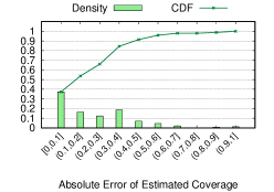
(a) TPC-H

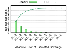
(b) TPC-DS

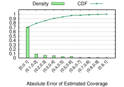
(c) Real-D

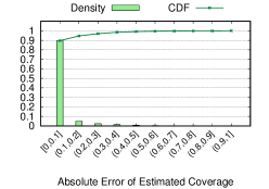
(d) Real-M

Figure 21. Error distributions of estimated coverage.

Figure 21 presents the probability distributions (both the probability density and the cumulative distribution function, i.e., CDF) for absolute errors on the workloads that we tested. We observe that, for 66%, 87%, 85%, and 97% of the query-index pairs collected on TPC-H, TPC-DS, Real-D, and Real-M, their absolute errors of the estimated coverage are below 0.3. The mean absolute errors observed on these workloads are 0.21, 0.16, 0.10, and 0.04, respectively. Based on Equation 4, since we further sum up the MCI’s to compute the lower bound, the aggregated error contributed to the lower bound when incorporating coverage-based refinement can be even smaller due to cancellation of the estimation errors made on individual MCI’s.

B.2. Cost Function Properties

We validate the monotonicity and submodularity assumptions of query optimizer cost functions.

Input: $W$, the workload.

Output: $D_{m}$, data points for monotonicity validation; $D_{s}$, data points for submodularity validation.

1 foreach query $q\in W$ do

2    Run vanilla greedy on $\{q\}$ with $K=2$ and $B=\infty$;

3    foreach candidate index $z$ of $q$ do

4       Collect all parent configurations $P_{z}=\{x,z\}$ of $z$ with known what-if costs;

5       foreach parent configuration $P_{z}$ do

6          Add three tuples $[c(q,\emptyset),c(q,\{z\})]$, $[c(q,\emptyset),c(q,P_{z})]$, and $[c(q,\{z\}),c(q,P_{z})]$ into $D_{m}$ for monotonicity check;

7          Add one tuple $[c(q,\emptyset),c(q,\{z\}),c(q,\{x\}),c(q,P_{z})]$ into $D_{s}$ for submodularity check;

8         

9return $D_{m}$ and $D_{s}$;

Algorithm 6 Collect data points for validation of cost function properties (i.e., monotonicity and submodularity).

For each workload, we collect data points using Algorithm 6. It runs vanilla greedy for each query $q$ (by viewing $q$ as a singleton workload) without a budget on the number of what-if calls. As a result, the actual what-if cost is used for every query-configuration pair. Since this step is costly, we limit the cardinality constraint to $K=2$ (line 2). After vanilla greedy finishes, Algorithm 6 iterates over each candidate index $z$ of the query $q$ to collect corresponding data points for checking monotonicity and submodularity (lines 3 to 8). For a given candidate index $z$ (i.e., a singleton configuration $\{z\}$), it looks for all of its parent configurations $P_{z}$, which contain $z$ and one additional candidate index $x$. At this point, we know $c(q,P_{z})$, $c(q,\{z\})$, $c(q,\{x\})$, and $c(q,\emptyset)$:

• For monotonicity validation, we check if (1) $c(q,\emptyset)\geq c(q,\{z\})$, (2) $c(q,\emptyset)\geq c(q,\{x,z\})$, and (3) $c(q,\{z\})\geq c(q,\{x,z\})$ (line 6). Note that we do not need to check whether $c(q,\emptyset)\geq c(q,\{x\})$ and $c(q,\{x\})\geq c(q,\{x,z\})$ here, since $x$ will also be visited by the iteration at sometime.

• For submodularity validation, we check if $c(q,\emptyset)-c(q,\{z\})\geq c(q,\{x\})-c(q,\{x,z\})$ (line 7).

Workload	# Total	# Yes	# No	% Yes	% No
TPC-H	1,132	1,121	11	99.0%	1.0%
TPC-DS	7,893	7,802	91	98.9%	1.1%
Real-D	7,808	7,668	140	98.2%	1.8%
Real-M	120,732	115,222	5,510	95.4%	4.6%

Table 5. Validation Results of Monotonicity Assumption.

Workload	# Total	# Yes	# No	% Yes	% No
TPC-H	444	389	55	87.6%	12.4%
TPC-DS	3,120	2,349	771	75.3%	24.7%
Real-D	3,282	2,896	386	88.2%	11.8%
Real-M	48,166	40,976	7,190	85.1%	14.9%

Table 6. Validation Results of Submodularity Assumption.

(a) TPC-H

(b) TPC-DS

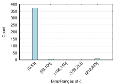
(c) Real-D

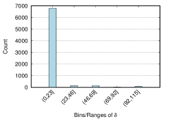
(d) Real-M

Figure 22. Histograms of $\delta$ when $\delta>0$.

Tables 5 and 6 present validation results of the monotonicity and submodularity assumptions, respectively. We report the number of data points collected by Algorithm 6 for each validation test (# Total), the number (resp. percentage) of data points where monotonicity/submodularity holds (# Yes resp. % Yes), and the number (resp. percentage) of data points where monotonicity/submodularity does not hold (# No resp. % No). We observe that the probability for monotonicity and submodularity to hold is high on all the workloads that we tested, whereas monotonicity holds with a higher probability ($\geq$95.4%) than submodularity ($\geq$75.3%).

We further looked into the cases where submodularity does not hold, by measuring the difference $\delta$ between $\delta(q,z,\emptyset)=c(q,\emptyset)-c(q,\{z\})$ and $\delta(q,z,\{x\})=c(q,\{x\})-c(q,\{x,z\})$. That is, $\delta=\delta(q,z,\{x\})-\delta(q,z,\emptyset).$ Intuitively, a violation of submodularity means $\delta>0$, and we call $\delta$ the magnitude of violation. Figure 22 presents the histograms for the data points collected on the workloads with $\delta>0$. We observe the same pattern for all the workloads tested: the distribution of $\delta$ (when $\delta>0$) is highly skewed, concentrating on regions where $\delta$ is small.

Appendix C Impact of Coverage on the Confidence

When we consider using “coverage” to estimate the what-if cost $c(q,{z})$ for a singleton configuration $\{z\}$ and thus the corresponding MCI upper-bound $u(q,z)$, the lower bound $L(q,C)$ becomes an estimated value as well. In the following, we use $\hat{c}(q,{z})$, $\hat{u}(q,z)$, and $\hat{L}(q,C)$ to denote the estimated values based on the estimated coverage $\rho(q,z)$. We present a quantitative analysis regarding the impact of using these estimated values in the confidence-based what-if call skipping mechanism.

By the definition of coverage, we have

$$c(q,\{z\})=c(q,\emptyset)-\rho(q,z)\cdot\Big{(}c(q,\emptyset)-c(q,\Omega_{q})\Big{)}=\Big{(}1-\rho(q,z)\Big{)}\cdot c(q,\emptyset)+\rho(q,z)\cdot c(q,\Omega_{q}).$$

As a result, it follows that

$$\hat{c}(q,\{z\})=c(q,\emptyset)-\hat{\rho}(q,z)\cdot\Big{(}c(q,\emptyset)-c(q,\Omega_{q})\Big{)}=\Big{(}1-\hat{\rho}(q,z)\Big{)}\cdot c(q,\emptyset)+\hat{\rho}(q,z)\cdot c(q,\Omega_{q}).$$

Now, assuming $u(q,z)=c(q,\emptyset)-c(q,\{z\})$, the estimated lower bound becomes

$$\hat{L}(q,C) = c(q,\emptyset)-\sum\nolimits_{z\in C}\hat{u}(q,z)$$

$$= c(q,\emptyset)-\sum\nolimits_{z\in C}\Big{(}c(q,\emptyset)-\hat{c}(q,\{z\})\Big{)}$$

$$= c(q,\emptyset)-\sum\nolimits_{z\in C}\hat{\rho}(q,z)\cdot\Big{(}c(q,\emptyset)-c(q,\Omega_{q})\Big{)}$$

$$= c(q,\emptyset)-\Delta(q,\Omega_{q})\cdot\sum\nolimits_{z\in C}\hat{\rho}(q,z).$$

It then follows that the confidence with coverage-based singleton cost estimates is

$$\hat{\alpha}(q,C)=\frac{\hat{L}(q,C)}{U(q,C)}=\frac{c(q,\emptyset)-\Delta(q,\Omega_{q})\cdot\sum\nolimits_{z\in C}\hat{\rho}(q,z)}{U(q,C)}.$$

On the other hand, by the definition of confidence we have

$$\alpha(q,C)=\frac{L(q,C)}{U(q,C)}=\frac{c(q,\emptyset)-\Delta(q,\Omega_{q})\cdot\sum\nolimits_{z\in C}\rho(q,z)}{U(q,C)}.$$

Combining the above two equations yields

$$U(q,C)\cdot\Big{(}\hat{\alpha}(q,C)-\alpha(q,C)\Big{)}=\Delta(q,\Omega_{q})\cdot\sum\nolimits_{z\in C}\Big{(}\rho(q,z)-\hat{\rho}(q,z)\Big{)}.$$

Or equivalently,

$$\alpha(q,C) = \hat{\alpha}(q,C)-\frac{\Delta(q,\Omega_{q})}{U(q,C)}\cdot\sum\nolimits_{z\in C}\Big{(}\rho(q,z)-\hat{\rho}(q,z)\Big{)}$$

$$= \hat{\alpha}(q,C)+\frac{\Delta(q,\Omega_{q})}{U(q,C)}\cdot\sum\nolimits_{z\in C}\Big{(}\hat{\rho}(q,z)-\rho(q,z)\Big{)}.$$

This implies that the degree of error in the confidence computation using estimated coverage depends on the sum of the errors made in estimating coverage for individual indexes (i.e., singleton configurations) within the configuration $C$.

References

- (1)
- dta (2023) 2023. DTA utility. https://docs.microsoft.com/en-us/sql/tools/dta/dta-utility?view=sql-server-ver15.
- Akdere et al. (2012) Mert Akdere, Ugur Çetintemel, Matteo Riondato, Eli Upfal, and Stanley B. Zdonik. 2012. Learning-based Query Performance Modeling and Prediction. In ICDE. 390–401.
- Browne et al. (2012) Cameron Browne, Edward Jack Powley, Daniel Whitehouse, Simon M. Lucas, Peter I. Cowling, Philipp Rohlfshagen, Stephen Tavener, Diego Perez Liebana, Spyridon Samothrakis, and Simon Colton. 2012. A Survey of Monte Carlo Tree Search Methods. IEEE Trans. Comput. Intell. AI Games 4, 1 (2012), 1–43.
- Brucato et al. (2024) Matteo Brucato, Tarique Siddiqui, Wentao Wu, Vivek Narasayya, and Surajit Chaudhuri. 2024. Wred: Workload Reduction for Scalable Index Tuning. Proc. ACM Manag. Data 2, 1, Article 50 (2024), 26 pages.
- Bruno and Chaudhuri (2005) Nicolas Bruno and Surajit Chaudhuri. 2005. Automatic Physical Database Tuning: A Relaxation-based Approach. In SIGMOD. 227–238.
- Chaudhuri et al. (2004) Surajit Chaudhuri, Mayur Datar, and Vivek R. Narasayya. 2004. Index Selection for Databases: A Hardness Study and a Principled Heuristic Solution. IEEE Trans. Knowl. Data Eng. 16, 11 (2004), 1313–1323.
- Chaudhuri and Narasayya (2020) Surajit Chaudhuri and Vivek Narasayya. 2020. Anytime Algorithm of Database Tuning Advisor for Microsoft SQL Server.
- Chaudhuri and Narasayya (1997) Surajit Chaudhuri and Vivek R. Narasayya. 1997. An Efficient Cost-Driven Index Selection Tool for Microsoft SQL Server. In VLDB. 146–155.
- Chaudhuri and Narasayya (1998) Surajit Chaudhuri and Vivek R. Narasayya. 1998. AutoAdmin ’What-if’ Index Analysis Utility. In SIGMOD. 367–378.
- Choenni et al. (1993) Sunil Choenni, Henk M. Blanken, and Thiel Chang. 1993. On the Selection of Secondary Indices in Relational Databases. Data Knowl. Eng. 11, 3 (1993).
- Comer (1978) Douglas Comer. 1978. The Difficulty of Optimum Index Selection. ACM Trans. Database Syst. 3, 4 (1978), 440–445.
- Dash et al. (2011) Debabrata Dash, Neoklis Polyzotis, and Anastasia Ailamaki. 2011. CoPhy: A Scalable, Portable, and Interactive Index Advisor for Large Workloads. Proc. VLDB Endow. 4, 6 (2011), 362–372.
- Ding et al. (2019) Bailu Ding, Sudipto Das, Ryan Marcus, Wentao Wu, Surajit Chaudhuri, and Vivek R. Narasayya. 2019. AI Meets AI: Leveraging Query Executions to Improve Index Recommendations. In SIGMOD. 1241–1258.
- Ganapathi et al. (2009) Archana Ganapathi, Harumi A. Kuno, Umeshwar Dayal, Janet L. Wiener, Armando Fox, Michael I. Jordan, and David A. Patterson. 2009. Predicting Multiple Metrics for Queries: Better Decisions Enabled by Machine Learning. In ICDE.
- Gupta et al. (1997) Himanshu Gupta, Venky Harinarayan, Anand Rajaraman, and Jeffrey D. Ullman. 1997. Index Selection for OLAP. In ICDE. 208–219.
- Hilprecht and Binnig (2022) Benjamin Hilprecht and Carsten Binnig. 2022. Zero-Shot Cost Models for Out-of-the-box Learned Cost Prediction. Proc. VLDB Endow. 15, 11 (2022), 2361–2374.
- Kane (2017) Andrew Kane. 2017. Introducing Dexter, the Automatic Indexer for Postgres. https://medium.com/@ankane/introducing-dexter-the-automatic-indexer-for-postgres-5f8fa8b28f27.
- Kocsis and Szepesvári (2006) Levente Kocsis and Csaba Szepesvári. 2006. Bandit Based Monte-Carlo Planning. In ECML. 282–293.
- Kossmann et al. (2020) Jan Kossmann, Stefan Halfpap, Marcel Jankrift, and Rainer Schlosser. 2020. Magic mirror in my hand, which is the best in the land? An Experimental Evaluation of Index Selection Algorithms. Proc. VLDB Endow. 13, 11 (2020), 2382–2395.
- Kossmann et al. (2022) Jan Kossmann, Alexander Kastius, and Rainer Schlosser. 2022. SWIRL: Selection of Workload-aware Indexes using Reinforcement Learning. In EDBT. 2:155–2:168.
- Lan et al. (2020) Hai Lan, Zhifeng Bao, and Yuwei Peng. 2020. An Index Advisor Using Deep Reinforcement Learning. In CIKM. 2105–2108.
- Leis et al. (2015) Viktor Leis, Andrey Gubichev, Atanas Mirchev, Peter A. Boncz, Alfons Kemper, and Thomas Neumann. 2015. How Good Are Query Optimizers, Really? Proc. VLDB Endow. 9, 3 (2015), 204–215.
- Li et al. (2012) Jiexing Li, Arnd Christian König, Vivek R. Narasayya, and Surajit Chaudhuri. 2012. Robust Estimation of Resource Consumption for SQL Queries using Statistical Techniques. Proc. VLDB Endow. 5, 11 (2012), 1555–1566.
- Marcus et al. (2019) Ryan C. Marcus, Parimarjan Negi, Hongzi Mao, Chi Zhang, Mohammad Alizadeh, Tim Kraska, Olga Papaemmanouil, and Nesime Tatbul. 2019. Neo: A Learned Query Optimizer. Proc. VLDB Endow. 12, 11 (2019), 1705–1718.
- Marcus and Papaemmanouil (2019) Ryan C. Marcus and Olga Papaemmanouil. 2019. Plan-Structured Deep Neural Network Models for Query Performance Prediction. Proc. VLDB Endow. 12, 11 (2019), 1733–1746.
- Papadomanolakis et al. (2007) Stratos Papadomanolakis, Debabrata Dash, and Anastassia Ailamaki. 2007. Efficient Use of the Query Optimizer for Automated Database Design. ACM.
- Paul et al. (2021) Debjyoti Paul, Jie Cao, Feifei Li, and Vivek Srikumar. 2021. Database Workload Characterization with Query Plan Encoders. Proc. VLDB Endow. 15, 4 (2021), 923–935.
- Perera et al. (2021) R. Malinga Perera, Bastian Oetomo, Benjamin I. P. Rubinstein, and Renata Borovica-Gajic. 2021. DBA bandits: Self-driving index tuning under ad-hoc, analytical workloads with safety guarantees. In ICDE. IEEE, 600–611.
- Perera et al. (2022) R. Malinga Perera, Bastian Oetomo, Benjamin I. P. Rubinstein, and Renata Borovica-Gajic. 2022. HMAB: Self-Driving Hierarchy of Bandits for Integrated Physical Database Design Tuning. Proc. VLDB Endow. 16, 2 (2022), 216–229.
- Schlosser et al. (2019) Rainer Schlosser, Jan Kossmann, and Martin Boissier. 2019. Efficient Scalable Multi-attribute Index Selection Using Recursive Strategies. In ICDE. 1238–1249.
- Schnaitter et al. (2009) Karl Schnaitter, Neoklis Polyzotis, and Lise Getoor. 2009. Index Interactions in Physical Design Tuning: Modeling, Analysis, and Applications. Proc. VLDB Endow. 2, 1 (2009), 1234–1245.
- Sharma et al. (2018) Ankur Sharma, Felix Martin Schuhknecht, and Jens Dittrich. 2018. The Case for Automatic Database Administration using Deep Reinforcement Learning. CoRR abs/1801.05643 (2018).
- Shi et al. (2022) Jiachen Shi, Gao Cong, and Xiaoli Li. 2022. Learned Index Benefits: Machine Learning Based Index Performance Estimation. Proc. VLDB Endow. 15, 13 (2022), 3950–3962.
- Siddiqui et al. (2020) Tarique Siddiqui, Alekh Jindal, Shi Qiao, Hiren Patel, and Wangchao Le. 2020. Cost Models for Big Data Query Processing: Learning, Retrofitting, and Our Findings. In SIGMOD. ACM, 99–113.
- Siddiqui et al. (2022a) Tarique Siddiqui, Saehan Jo, Wentao Wu, Chi Wang, Vivek R. Narasayya, and Surajit Chaudhuri. 2022a. ISUM: Efficiently Compressing Large and Complex Workloads for Scalable Index Tuning. In SIGMOD. ACM, 660–673.
- Siddiqui and Wu (2023) Tarique Siddiqui and Wentao Wu. 2023. ML-Powered Index Tuning: An Overview of Recent Progress and Open Challenges. SIGMOD Rec. 52, 4 (2023), 19–30.
- Siddiqui et al. (2022b) Tarique Siddiqui, Wentao Wu, Vivek R. Narasayya, and Surajit Chaudhuri. 2022b. DISTILL: Low-Overhead Data-Driven Techniques for Filtering and Costing Indexes for Scalable Index Tuning. Proc. VLDB Endow. 15, 10 (2022), 2019–2031.
- Sun and Li (2019) Ji Sun and Guoliang Li. 2019. An End-to-End Learning-based Cost Estimator. Proc. VLDB Endow. 13, 3 (2019), 307–319.
- Sutton and Barto (2018) Richard S Sutton and Andrew G Barto. 2018. Reinforcement learning: An introduction. MIT press.
- Valentin et al. (2000) Gary Valentin, Michael Zuliani, Daniel C. Zilio, Guy M. Lohman, and Alan Skelley. 2000. DB2 Advisor: An Optimizer Smart Enough to Recommend Its Own Indexes. In ICDE. 101–110.
- Wang et al. (2024) Xiaoying Wang, Wentao Wu, Chi Wang, Vivek Narasayya, and Surajit Chaudhuri. 2024. Wii: Dynamic Budget Reallocation In Index Tuning (Extended Version). Technical Report. Microsoft Research. https://www.microsoft.com/en-us/research/people/wentwu/publications/
- Whang (1985) Kyu-Young Whang. 1985. Index Selection in Relational Databases. In Foundations of Data Organization. 487–500.
- Wu et al. (2013a) Wentao Wu, Yun Chi, Hakan Hacigümüs, and Jeffrey F. Naughton. 2013a. Towards Predicting Query Execution Time for Concurrent and Dynamic Database Workloads. Proc. VLDB Endow. 6, 10 (2013), 925–936.
- Wu et al. (2013b) Wentao Wu, Yun Chi, Shenghuo Zhu, Jun’ichi Tatemura, Hakan Hacigümüs, and Jeffrey F. Naughton. 2013b. Predicting query execution time: Are optimizer cost models really unusable?. In ICDE. 1081–1092.
- Wu et al. (2016) Wentao Wu, Jeffrey F. Naughton, and Harneet Singh. 2016. Sampling-Based Query Re-Optimization. In SIGMOD. ACM, 1721–1736.
- Wu et al. (2022) Wentao Wu, Chi Wang, Tarique Siddiqui, Junxiong Wang, Vivek R. Narasayya, Surajit Chaudhuri, and Philip A. Bernstein. 2022. Budget-aware Index Tuning with Reinforcement Learning. In SIGMOD. ACM, 1528–1541.
- Wu et al. (2014) Wentao Wu, Xi Wu, Hakan Hacigümüs, and Jeffrey F. Naughton. 2014. Uncertainty Aware Query Execution Time Prediction. Proc. VLDB Endow. 7, 14 (2014), 1857–1868.
- Zhao et al. (2022) Yue Zhao, Gao Cong, Jiachen Shi, and Chunyan Miao. 2022. QueryFormer: A Tree Transformer Model for Query Plan Representation. Proc. VLDB Endow. 15, 8 (2022), 1658–1670.