Schmidt number criterion via symmetric measurements

Abstract

The Schmidt numbers quantify the entanglement dimension of quantum states. We derive a Schmidt number criterion based on the trace norm of the correlation matrix obtained from symmetric measurements. We show that our Schmidt number criterion is more effective than and superior to existing criteria by detailed examples.

I Introduction

An important issue in the theory of quantum entanglement is the quantification and estimation of entanglement for composite systems. The Schmidt number is a well-known quantification of bipartite entanglement Terhal ; Sperling , which shows that a quantum state is separable if and only if it’s Schmidt number is one. Bipartite quantum states with higher Schmidt numbers are generally considered superior to those with lower Schmidt numbers in various information processing tasks. For example, it has been shown in Bae that quantum states with higher Schmidt numbers have certain advantages in channel discrimination.

Due to the importance of Schmidt numbers, how to effectively detect the Schmidt number of a given state has become a fundamental problem. The first Schmidt number criterion is obtained by examining the fidelity between the quantum state and the maximally entangled states Terhal . Then in Hulpke ; Johnston the authors presented a Schmidt number criterion by generalizing the well-known positive partial transpose (PPT) PPT1 ; PPT2 and the computable cross-norm or realignment criterion (CCNR) CCNR1 ; CCNR2 criteria. Later, the Schmidt number criteria based on Bloch decomposition Klockl and covariance matrix Liu1 ; Liu2 have been derived respectively. In addition, a witness-based method has also been developed to detect the Schmidt number of a stateSanpera ; Wyderka ; Shi . Recently, the authors in Ref.Tavakoli proposed two elegant criteria to detect the Schmidt number based on the correlation matrix obtained from symmetric informationally complete measure (SIC POVM) and from mutually unbiased bases (MUBs). The results are generalized to the one based on general SIC POVM (GSIC POVM) ZWang , as a generalization of the entanglement criterion given in Ref.Lai .

It is well-known that mutually unbiased measurements (MUMs) and GSIC POVM are the natural extensions of MUBs and SIC POVM, respectively. Recently, the symmetric measurement or $(N,M)$-POVM has been proposed Siudzinska , which includes MUMs and GSIC POVM as special cases.

In this work, we derive a criterion of Schmidt number detection based on the trace norm of the correlation matrix whose entries are obtained via symmetric measurements. It can be considered as a generalization of the GSIC criterion ZWang and the MUB criterion Tavakoli . We show that our criterion is more efficient in detecting the Schmidt number than some existing criteria by detailed examples. Moreover, from the proof of our criterion of Schmidt number, we also obtain a class of lower bounds of concurrence induced by symmetric measurements, which generalizes the results given in Ref.Haofan .

II Symmetric measurement based Schmidt number criterion

We first recall the $(N,M)$-POVM. A set of $N$ $d$-dimensional POVMs $\{E_{\alpha,k}|k=1,2\cdots,M\}$ ($\alpha=1,2,\cdots,N$) constitute an $(N,M)$-POVM if

$${\rm tr}(E_{\alpha,k}) =\dfrac{d}{M},$$

$${\rm tr}(E_{\alpha,k}^{2}) =x,$$

$${\rm tr}(E_{\alpha,k}E_{\alpha,l}) =\dfrac{d-Mx}{M(M-1)},~~l\neq k$$

$${\rm tr}(E_{\alpha,k}E_{\beta,l}) =\dfrac{d}{M^{2}},~~\beta\neq\alpha$$

where the parameter $x$ satisfies $\dfrac{d}{M^{2}}<x\leq\min\left\{\dfrac{d^{2}}{M^{2}},\dfrac{d}{M}\right\}$. When $N(M-1)=d^{2}-1$, the $(N,M)$-POVM is called an informationally complete $(N,M)$-POVM. For any finite dimension $d$ ($d>2$), there exist at least four different types of informationally complete $(N,M)$-POVM: (1) $N=1$ and $M=d^{2}$ (GSIC POVM), (2) $N=d+1$ and $M=d$ (MUMs), (3) $N=d^{2}-1$ and $M=2$, (4) $N=d-1$ and $M=d+2$.

From orthonormal Hermitian operator basis $\{G_{0}=I_{d}/\sqrt{d},\,G_{\alpha,k}|\alpha=1,\cdots,N;\,k=1,\cdots,M-1\}$ with ${\rm tr}(G_{\alpha,k})=0$, an informationally complete $(N,M)$-POVM is given by

$$E_{\alpha,k}=\dfrac{1}{M}I_{d}+tH_{\alpha,k},$$

where

$$H_{\alpha,k}=\begin{cases}G_{\alpha}-\sqrt{M}(\sqrt{M}+1)G_{\alpha,k},~k=1,\cdots,M-1\\ (\sqrt{M}+1)G_{\alpha},k=M\end{cases}$$

with $G_{\alpha}=\sum\limits_{k=1}^{M-1}G_{\alpha,k}$. The parameter $t$ should be chosen such that $E_{\alpha,k}\geq 0$, which implies that

$$-\dfrac{1}{M}\dfrac{1}{\lambda_{\max}}\leq t\leq\dfrac{1}{M}\dfrac{1}{|\lambda_{\min}|},$$

where $\lambda_{\max}$ and $\lambda_{\min}$ are the minimal and maximal eigenvalues of $H_{\alpha,k}$ for all $\alpha$ and $k$, respectively. The parameters $t$ and $x$ satisfy the following relation,

$$x=\dfrac{d}{M^{2}}+t^{2}(M-1)(\sqrt{M}+1)^{2}.$$

A bipartite pure state $\ket{\psi}\in\mathcal{H}_{A}\otimes\mathcal{H}_{B}$ has a Schmidt decomposition $\ket{\psi}=\sum\limits_{i=1}^{r}\lambda_{i}\ket{e_{i}f_{i}}$, where $\lambda_{i}>0$ and $\sum\limits_{i=1}^{r}\lambda_{i}^{2}=1$, $\{\ket{e_{i}}\}$ and $\{\ket{f_{i}}\}$ are the orthonormal bases in $\mathcal{H}_{A}$ and $\mathcal{H}_{B}$, respectively. The number $r$ is called the Schmidt rank of $\ket{\psi}$, denoted as ${\rm SR}(\ket{\psi})$. The Schmidt number of a bipartite mixed state $\rho$ in $\mathcal{H}_{A}\otimes\mathcal{H}_{B}$ is defined as

$${\rm SN}(\rho)=\min\limits_{\{p_{i},\ket{\psi_{i}}\}}\max\limits_{i}{\rm SR}(\ket{\psi_{i}}),$$

where the minimization goes over all possible pure state decompositions of $\rho=\sum_{i}p_{i}\ket{\psi_{i}}\bra{\psi_{i}}$.

Lemma 1.

Let $\{E_{\alpha,k}|\alpha=1,\cdots,N;\,k=1,\cdots,M\}$ be an informationally complete $(N,M)$-POVM on $d$ dimensional Hilbert space $\mathcal{H}$ with free parameter $x$. Then for any linear operator $\sigma\in L(\mathcal{H})$, we have

$$\sum_{\alpha=1}^{N}\sum_{k=1}^{M}|{\rm tr}(E_{\alpha,k}\sigma)|^{2}=\dfrac{d(M^{2}x-d){\rm tr}(\sigma\sigma^{\dagger})+(d^{3}-M^{2}x)|{\rm tr}(\sigma)|^{2}}{dM(M-1)}.$$

Proof.

Denote $w=\dfrac{d}{M}$, $y=\dfrac{d-Mx}{M(M-1)}$ and $z=\dfrac{d}{M^{2}}$. For any linear operator $\sigma\in L(\mathcal{H})$, we can verify that

$$\sigma=\sum\limits_{\alpha=1}^{N}\sum\limits_{k=1}^{M}{\rm tr}(E_{\alpha,k}\sigma)F_{\alpha,k},$$

where $F_{\alpha,k}=\dfrac{1}{x-y}\left(E_{\alpha,k}-\dfrac{(N-1)z+y}{Nw}I\right)$. Define $p_{\alpha,k}={\rm tr}(E_{\alpha,k}\sigma)$. Then

$${\rm tr}(\sigma\sigma^{\dagger})=\sum\limits_{\alpha,\beta=1}^{N}\sum\limits_{k,l=1}^{M}p_{\alpha,k}\overline{p_{\beta,l}}{\rm tr}(F_{\alpha,k}F_{\beta,l}).$$

By definition it follows that

$${\rm tr}(F_{\alpha,k}F_{\beta,l})=\dfrac{1}{(x-y)^{2}}\left[{\rm tr}(E_{\alpha,k}E_{\beta,l})+A(dA-2w)\right],$$

where $A=\dfrac{(N-1)z+y}{Nw}$. As a result, we have

$$\begin{array}[]{ll}{\rm tr}(\sigma\sigma^{\dagger})&=\dfrac{1}{(x-y)^{2}}\Bigg{[}\sum\limits_{\alpha=1}^{N}\sum\limits_{k=1}^{M}|p_{\alpha,k}|^{2}{\rm tr}(E_{\alpha,k}^{2})+\sum\limits_{\alpha=1}^{N}\sum\limits_{\begin{subarray}{c}k,l=1\\ l\neq k\end{subarray}}^{M}p_{\alpha,k}\overline{p_{\alpha,l}}{\rm tr}(E_{\alpha,k}E_{\alpha,l})\\ &\qquad\qquad\quad+\sum\limits_{\begin{subarray}{c}\alpha,\beta=1\\ \beta\neq\alpha\end{subarray}}^{N}\sum\limits_{k,l=1}^{M}p_{\alpha,k}\overline{p_{\beta,l}}{\rm tr}(E_{\alpha,k}E_{\beta,l})+N^{2}A(dA-2w)|{\rm tr}(\sigma)|^{2}\Bigg{]}\\ &=\dfrac{1}{(x-y)^{2}}\left[Cx+Ny|{\rm tr}(\sigma)|^{2}-Cy+N(N-1)z|{\rm tr}(\sigma)|^{2}+N^{2}A(dA-2w)|{\rm tr}(\sigma)|^{2}\right]\\ &=\dfrac{1}{(x-y)^{2}}\left[(x-y)C+N(y+(N-1)z)|{\rm tr}(\sigma)|^{2}+N^{2}A(dA-2w)|{\rm tr}(\sigma)|^{2}\right]\\ &=\dfrac{1}{(x-y)^{2}}\left[(x-y)C+\left(N+\dfrac{(dA-2w)N}{w}\right)(y+(N-1)z)|{\rm tr}(\sigma)|^{2}\right]\\ &=\dfrac{dM(M-1)C+(M^{2}x-d^{3})|{\rm tr}(\sigma)|^{2}}{d(M^{2}x-d)},\end{array}$$

where $C=\sum\limits_{\alpha=1}^{N}\sum\limits_{k=1}^{M}|p_{\alpha,k}|^{2}$ and we have used $(M-1)N=d^{2}-1$ in the last equality. The proof of the lemma is completed by adjusting the above equation. ∎

Theorem 1.

Let $\{E_{\alpha,k}^{A}|\alpha=1,\cdots,N_{A};\,k=1,\cdots,M_{A}\}$ be an informationally complete $(N_{A},M_{A})$-POVM on Hilbert space $\mathcal{H}_{A}$ and $\{E_{\beta,l}^{B}|\beta=1,\cdots,N_{B};\,l=1,\cdots,M_{B}\}$ an informationally complete $(N_{B},M_{B})$-POVM on Hilbert space $\mathcal{H}_{B}$. Denote $p_{\alpha,k;\beta,l}={\rm tr}\left(\rho_{AB}\left(E_{\alpha,k}^{A}\otimes E_{\beta,l}^{B}\right)\right)$ and $\mathcal{P}(\rho_{AB})=\left(p_{\alpha,k;\beta,l}\right)_{N_{A}M_{A}\times N_{B}M_{B}}$ for a bipartite state $\rho_{AB}$ in $\mathcal{H}_{A}\otimes\mathcal{H}_{B}$. If the Schmidt number of $\rho_{AB}$ is at most $r$, it holds that

$$\|\mathcal{P}(\rho_{AB})\|_{\rm tr}\leq\dfrac{L}{K}+(r-1)\dfrac{R}{K},$$

where

$$K = \sqrt{d_{A}d_{B}(M_{A}-1)(M_{B}-1)},$$

$$L = \sqrt{\dfrac{(d_{A}-1)(d_{B}-1)(M_{A}^{2}x_{A}+d_{A}^{2})(M_{B}^{2}x_{B}+d_{B}^{2})}{M_{A}M_{B}}},$$

$$R = \sqrt{\dfrac{d_{A}d_{B}(M_{A}^{2}x_{A}-d_{A})(M_{B}^{2}x_{B}-d_{B})}{M_{A}M_{B}}}.$$

Proof.

Since the trace norm is convex, without loss of generality, instead of mixed states we consider pure states with Schmidt rank $r$, $\ket{\psi}=\sum\limits_{s=1}^{r}\lambda_{s}\ket{ss}$, where $\{\lambda_{s}\}$ is the set of Schmidt coefficients with $\sum\limits_{s=1}^{r}\lambda_{s}^{2}=1$. As a result, we obtain

$$\begin{array}[]{ll}{\rm tr}\left(\ket{\psi}\bra{\psi}\left(E_{\alpha,k}^{A}\otimes E_{\beta,l}^{B}\right)\right)&=\sum\limits_{s,t=1}^{r}\lambda_{s}\lambda_{t}\braket{ss|E_{\alpha,k}^{A}\otimes E_{\beta,l}^{B}|tt}\\ &=\sum\limits_{s=1}^{r}\lambda_{s}^{2}\braket{ss|E_{\alpha,k}^{A}\otimes E_{\beta,l}^{B}|ss}+\sum\limits_{s\neq t}\lambda_{s}\lambda_{t}\braket{ss|E_{\alpha,k}^{A}\otimes E_{\beta,l}^{B}|tt}.\end{array}$$ (3)

Define $[D_{s}]_{\alpha,k;\beta,l}=\braket{ss|E_{\alpha,k}^{A}\otimes E_{\beta,l}^{B}|ss}$ and $[O_{s,t}]_{\alpha,k;\beta,l}=\braket{ss|E_{\alpha,k}^{A}\otimes E_{\beta,l}^{B}|tt}$. It then follows that

$$\|D_{s}\|_{\rm tr} = \sqrt{\sum\limits_{\alpha=1}^{N_{A}}\sum\limits_{k=1}^{M_{A}}\braket{s|E_{\alpha,k}|s}^{2}}\sqrt{\sum\limits_{\beta=1}^{N_{B}}\sum\limits_{l=1}^{M_{B}}\braket{s|E_{\beta,l}|s}^{2}},$$

$$\|O_{s,t}\|_{\rm tr} = \sqrt{\sum\limits_{\alpha=1}^{N_{A}}\sum\limits_{k=1}^{M_{A}}|\braket{s|E_{\alpha,k}|t}|^{2}}\sqrt{\sum\limits_{\beta=1}^{N_{B}}\sum\limits_{l=1}^{M_{B}}|\braket{s|E_{\beta,l}|t}|^{2}},~~~s\neq t.$$

Using Lemma 1, we obtain

$$\|D_{s}\|_{\rm tr} = \sqrt{\dfrac{(d_{A}-1)(M_{A}^{2}x_{A}+d_{A}^{2})}{d_{A}M_{A}(M_{A}-1)}}\sqrt{\dfrac{(d_{B}-1)(M_{B}^{2}x_{B}+d_{B}^{2})}{d_{B}M_{B}(M_{B}-1)}},$$

$$\|O_{s,t}\|_{\rm tr} = \sqrt{\dfrac{M_{A}^{2}x_{A}-d_{A}}{M_{A}(M_{A}-1)}}\sqrt{\dfrac{M_{B}^{2}x_{B}-d_{B}}{M_{B}(M_{B}-1)}},~~~s\neq t.$$

From Eq. (3), we obtain

$$\begin{array}[]{ll}\|\mathcal{P}(\ket{\psi}\bra{\psi})\|_{\rm tr}&\leq\sum\limits_{s=1}^{r}\lambda_{s}^{2}\|D_{s}\|_{\rm tr}+\sum\limits_{s\neq t}\lambda_{s}\lambda_{t}\|O_{s,t}\|_{\rm tr}\\ &=\dfrac{1}{K}\left[\left(\sum\limits_{s=1}^{r}\lambda_{s}^{2}\right)(L-R)+\left(\sum\limits_{s=1}^{r}\lambda_{s}\right)^{2}R\right]\\ &=\dfrac{L}{K}+\dfrac{R}{K}\left[\left(\sum\limits_{s=1}^{r}\lambda_{s}\right)^{2}-1\right].\end{array}$$ (7)

The proof of Theorem 1 is now complete by using the fact that $\left(\sum\limits_{s=1}^{r}\lambda_{s}\right)^{2}\leq r$Terhal . ∎

Remark 1.

If $\rho_{AB}$ is a separable, then ${\rm SN}(\rho_{AB})=1$. Consequently from Theorem 1 we have $\|\mathcal{P}(\rho_{AB})\|_{\rm tr}\leq\sqrt{\frac{(d_{A}-1)(M_{A}^{2}x_{A}+d_{A}^{2})}{d_{A}M_{A}(M_{A}-1)}}\sqrt{\frac{(d_{B}-1)(M_{B}^{2}x_{B}+d_{B}^{2})}{d_{B}M_{B}(M_{B}-1)}}$. Hence our Theorem 1 covers the entanglement criterion given in Ref. Siudzinska ; Tang .

Remark 2.

Set $M_{A}=d_{A}^{2}$, $M_{B}=d_{B}^{2}$ and $N_{A}=N_{B}=1$ in Theorem 1. Then

$$K = \sqrt{d_{A}d_{B}(d_{A}^{2}-1)(d_{B}^{2}-1)},$$

$$L = \sqrt{(d_{A}-1)(d_{B}-1)(x_{A}d_{A}^{2}+1)(x_{B}d_{B}^{2}+1)},$$

$$R = \sqrt{(x_{A}d_{A}^{3}-1)(x_{B}d_{B}^{3}-1)}.$$

Hence, Theorem 1 generalizes the GSIC Schmidt number criterion proposed in Ref.ZWang . Similarly, take $N_{A}-1=M_{A}=d_{A}$, $N_{B}-1=M_{B}=d_{B}$ and $x_{A}=x_{B}=1$. We obtain $K=\frac{1}{2}L=R=\sqrt{d_{A}d_{B}(d_{A}-1)(d_{B}-1)}$. Then $\|\mathcal{P}(\rho_{AB})\|_{\rm tr}\leq 1+r$. This indicates that Theorem 1 also generalizes the MUBs Schmidt number criterion given in Tavakoli .

Remark 3.

The concurrence of a bipartite state $\ket{\psi}$ is defined by $C(\ket{\psi})=\sqrt{2(1-{\rm tr}(\rho_{A}^{2}))}$, where $\rho_{A}={\rm tr}_{B}(\ket{\psi}\bra{\psi})$ is the reduced state obtained by tracing over the subsystem $B$. The concurrence of a mixed state $\rho_{AB}$ is given by the convex roof extension, $C(\rho_{AB})=\min\limits_{\{p_{i},\ket{\psi_{i}}\}}\sum\limits_{i}p_{i}C(\ket{\psi_{i}})$, where the minimum is taken over all possible pure state decompositions of $\rho_{AB}=\sum\limits_{i}p_{i}\ket{\psi_{i}}\bra{\psi_{i}}$, with $p_{i}\geq 0$ and $\sum\limits_{i}p_{i}=1$. Denote $d=\min\{d_{A},d_{B}\}$. According to Eq. (7), we obtain

$$\frac{K}{R}\left(\|\mathcal{P}(\ket{\psi}\bra{\psi})\|_{\rm tr}-\frac{L}{K}\right)\leq\left(\sum\limits_{i}\lambda_{i}\right)^{2}-1=2\sum\limits_{i<j}\lambda_{i}\lambda_{j},$$

from which we can prove that

$$C(\rho_{AB})\geq\frac{K}{R}\sqrt{\frac{2}{d(d-1)}}\left(\|\mathcal{P}(\rho_{AB})\|_{\rm tr}-\frac{L}{K}\right)$$ (8)

by using $C(\ket{\psi})\geq 2\sqrt{\dfrac{2}{d(d-1)}}\sum\limits_{i<j}\lambda_{i}\lambda_{j}$ Chen and the convex property of the trace norm. When $\mathcal{H}_{A}=\mathcal{H}_{B}$ and $(N_{A},M_{A})=(N_{B},M_{B})$, (8) reduces to the lower bound of concurrence given by Theorem 1 in Ref.Haofan .

Corollary 1.

Let $\{E_{\alpha,k}|\alpha=1,\cdots,N;\,k=1,\cdots,M\}$ be an informationally complete $(N,M)$-POVM on Hilbert space $\mathcal{H}$. Denote $p_{\alpha,k;\beta,l}={\rm tr}\left(\rho\left(E_{\alpha,k}\otimes E_{\beta,l}\right)\right)$ and $\mathcal{P}(\rho)=\left(p_{\alpha,k;\beta,l}\right)_{d^{2}\times d^{2}}$ $\rho$ for a bipartite state in $\mathcal{H}\otimes\mathcal{H}$. If the Schmidt number of $\rho$ is at most $r$, it holds that

$$\|\mathcal{P}(\rho)\|_{\rm tr}\leq\dfrac{(d-1)(M^{2}x+d^{2})}{dM(M-1)}+(r-1)\dfrac{M^{2}x-d}{M(M-1)}.$$

Remark 4.

Let $\ket{\psi}=\sum\limits_{i=1}^{r}\lambda_{i}\ket{ii}$ be a pure state in $\mathcal{H}\otimes\mathcal{H}$. Since $\left(\sum\limits_{i=1}^{r}\lambda_{i}\right)^{2}\leq r$ and $\sum\limits_{i=1}^{r}\lambda_{i}^{2}=1$, we have $r-1\geq 2\sum\limits_{i<j}\lambda_{i}\lambda_{j}$. Due to every informationally complete $(N,M)$-POVM is a conical 2-design Siudzinska2 ; Huang , we obtain Haofan

$$\dfrac{M(M-1)}{xM^{2}-d}\left(\|\mathcal{P}(\ket{\psi}\bra{\psi})\|_{\rm tr}-\dfrac{(d-1)(xM^{2}+d^{2})}{dM(M-1)}\right)=2\sum\limits_{i<j}\lambda_{i}\lambda_{j}\leq r-1.$$

This indicates that we have proven Corollary 1 in another way. This very meaningful observation implies that we can propose new Schmidt number criterion based on other new conical 2-designs.

Let us consider several examples to illustrate our conclusions.

Example 1.

Consider the following $2\otimes 4$ state, $\rho(\tau,q)=q\ket{\xi}\bra{\xi}+(1-q)\rho_{\tau}$, where $\rho_{\tau}$ is the bound entangled state proposed by Horodecki state ,

$$\rho_{\tau}=\dfrac{1}{1+7\tau}\begin{pmatrix}\tau&0&0&0&0&\tau&0&0\\ 0&\tau&0&0&0&0&\tau&0\\ 0&0&\tau&0&0&0&0&\tau\\ 0&0&0&\tau&0&0&0&0\\ 0&0&0&0&\frac{1+\tau}{2}&0&0&\frac{\sqrt{1-\tau^{2}}}{2}\\ \tau&0&0&0&0&\tau&0&0\\ 0&\tau&0&0&0&0&\tau&0\\ 0&0&\tau&0&\frac{\sqrt{1-\tau^{2}}}{2}&0&0&\frac{1+\tau}{2}\end{pmatrix}$$

with $0<\tau<1$ and $\ket{\xi}=\frac{1}{\sqrt{2}}(\ket{00}+\ket{11})$. We construct $(3,2)$-POVM with the Hermitian basis operators given by Pauli matrices $G_{11}=\dfrac{1}{\sqrt{2}}\begin{pmatrix}0&1\\ 1&0\\ \end{pmatrix}$,  $G_{21}=\dfrac{1}{\sqrt{2}}\begin{pmatrix}0&-\mathrm{i}\\ \mathrm{i}&0\\ \end{pmatrix}$,  $G_{31}=\dfrac{1}{\sqrt{2}}\begin{pmatrix}1&0\\ 0&-1\\ \end{pmatrix}$, and $(5,4)$-POVM with the Hermitian basis operators given by the general Gell-Mann matrices $G_{\alpha,k}$ for $\alpha=1,2,\cdots,5$ and $k=1,2,3$, see Appendix A. It is verified that the corresponding parameters $x_{1}=\frac{1}{2}+(\sqrt{2}+1)^{2}t_{1}^{2}$ with $t_{1}\in[-0.2929,0.2929]$ and $x_{2}=\frac{1}{4}+27t_{2}^{2}$ with $t_{2}\in[-0.0572,0.0680]$. We take $\rho=\rho(0.9,q)$. In Fig.1, the red curve is the value of $\frac{K}{R}(\|\mathcal{P}(\rho)\|_{\rm tr}-\frac{L}{K})$ from Theorem 1 based on $(3,2)$-POVM and $(5,4)$-POVM with $t_{1}=t_{2}=0.01$. The green curve is the value of $\frac{K}{R}(\|\mathcal{P}(\rho)\|_{\rm tr}-\frac{L}{K})$ based on GSIC POVMs with $a_{1}=0.1277$ and $a_{2}=0.04984$. In fact, the red curve shows that $\rho(0.9,q)$ is entangled for $0.42115\leq q\leq 1$, and the green curve fails to detect the entanglement of $\rho(0.9,q)$. Thus, our criterion is more efficient in detecting the Schmidt number than the GSIC criterion introduced in Ref.ZWang .

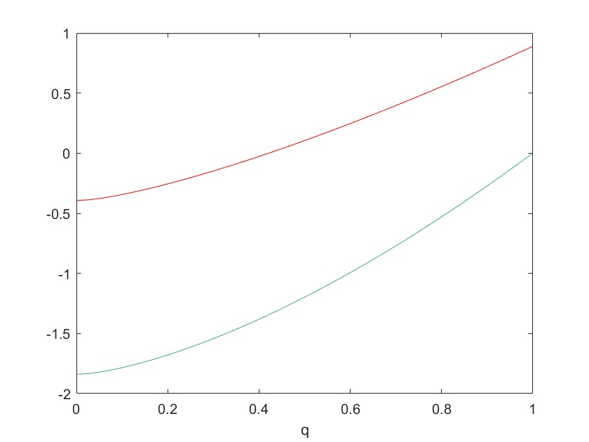
Figure 1: Red curve based on $(3,2)$-POVM and $(5,4)$-POVM. Green curve based on GSIC POVMs.

Example 2.

Consider the following isotropic state isostate ,

$$\rho_{v}=v\ket{\Psi^{+}}\bra{\Psi^{+}}+(1-v)\dfrac{I}{d^{2}},$$

where $I$ is the identity operator on ${H\otimes H}$, $\ket{\Psi^{+}}=\dfrac{1}{\sqrt{d}}\sum\limits_{i=1}^{d}\ket{ii}$ and $0<v<1$. It is easy to know that

$$\|\mathcal{P}(\rho_{v})\|_{\rm tr}=\dfrac{N}{M}+\dfrac{vN(M^{2}x-d)}{dM}=\dfrac{(d-1)(M^{2}x+d^{2})}{dM(M-1)}+\dfrac{N(M^{2}x-d)}{dM}\left(v-\dfrac{1}{d+1}\right)$$

by direct calculation Haofan . For the state $\rho_{v}$, the fidelity witness given in Terhal says that the visibility $v$ must be greater than the critical value $v_{\rm opt}=\frac{rd-1}{d^{2}-1}$ if the isotropic state has Schmidt number $r+1$. For any value of $v>v_{\rm opt}$ it holds that

$$\begin{array}[]{ll}\|\mathcal{P}(\rho_{v})\|_{\rm tr}&>\dfrac{(d-1)(M^{2}x+d^{2})}{dM(M-1)}+\dfrac{N(M^{2}x-d)}{dM}\left(\dfrac{rd-1}{d^{2}-1}-\dfrac{1}{d+1}\right)\\ &=\dfrac{(d-1)(M^{2}x+d^{2})}{dM(M-1)}+(r-1)\dfrac{M^{2}x-d}{M(M-1)}.\end{array}$$

Consequently, our criterion is stronger than the fidelity witness.

Example 3.

Consider the mixture of the bound entangled state considered in Ref.state ,

$$\rho_{\tau}=\dfrac{1}{1+8\tau}\begin{pmatrix}\tau&0&0&0&\tau&0&0&0&\tau\\ 0&\tau&0&0&0&0&0&0&0\\ 0&0&\tau&0&0&0&0&0&0\\ 0&0&0&\tau&0&0&0&0&0\\ \tau&0&0&0&\tau&0&0&0&\tau\\ 0&0&0&0&0&\tau&0&0&0\\ 0&0&0&0&0&0&\frac{1+\tau}{2}&0&\frac{\sqrt{1-\tau^{2}}}{2}\\ 0&0&0&0&0&0&0&0&0\\ \tau&0&0&0&\tau&0&\frac{\sqrt{1-\tau^{2}}}{2}&0&\frac{1+\tau}{2}\end{pmatrix}$$

and the $9\times 9$ identity matrix $I_{9}$,

$$\rho(\tau,q)=q\rho_{\tau}+\frac{1-q}{9}I_{9}.$$

Take the $(N,M)$-POVM in Corollary 1 to be $(8,2)$-POVM with the Hermitian basis operator $G_{\alpha,k}$ given in Appendix B. It is verified that the parameter $x=\frac{3}{4}+t^{2}(\sqrt{2}+1)^{2}$ with $t\in[-0.2536,0.2536]$. Consider $\rho=\rho(\tau,0.995)$. In Fig. 2, the red curve is the value of $\frac{M(M-1)}{xM^{2}-d}\left(\|\mathcal{P}(\rho)\|_{\rm tr}-\frac{(d-1)(xM^{2}+d^{2})}{dM(M-1)}\right)$ based on $(8,2)$-POVM with $t=0.01$. The green curve is the value of $\frac{d(d^{2}-1)}{ad^{3}-1}\left(\|\mathcal{P}(\rho)\|_{\rm tr}-\frac{ad^{2}+1}{d(d+1)}\right)$ based on GSIC POVM with $a=0.04984$. The purple curve is the value of $d(d+1)\left(\|\mathcal{P}(\rho)\|_{\rm tr}-\frac{2}{d(d+1)}\right)$ based on SIC POVM. The orange curve is the value of $\|\mathcal{R}(\rho)\|_{\rm tr}-1$, where $\mathcal{R}(\rho)$ is realigned matrix of $\rho$. It is seen that our criterion is more efficient in detecting the Schmidt number than other criteria.

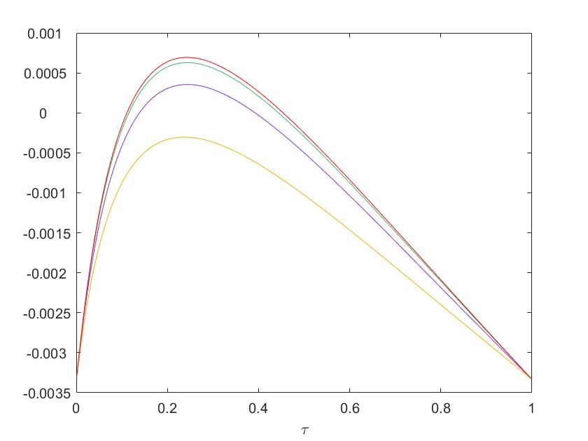
Figure 2: Red curve based on $(8,2)$-POVM, green curve based on GSIC POVM, purple curve based on SIC POVM, orange curve based on realignment.

III Conclusions and Discussions

We have provided a criterion for detecting the Schmidt numbers of bipartite states based on symmetric measurements. As symmetric measurements cover GSIC POVM and MUBs, our criterion includes the GSIC and MUBs based criteria as particular cases. We have illustrated that our criterion is more effective than and superior to the GSIC criterion, the fidelity criterion and the CCNR criterion. Moreover, we have obtained a class of symmetric measurement-induced lower bounds of concurrence for heterogeneous systems, which includes the one given in Ref.Haofan as particular cases. Our results may highlight further investigations on the Schmidt number criteria based on other quantum measurements or conical 2-designs.

Acknowlegements This work is supported by the National Natural Science Foundation of China (NSFC) under Grant No. 12171044; the specific research fund of the Innovation Platform for Academicians of Hainan Province.

Appendix A The Hermitian basis operators used to construct $(5,4)$-POVM in Example 1

In Example 1, we used $(5,4)$-POVM with the Hermitian basis operators $G_{\alpha,k}$ given by the following general Gell-Mann matrices:

$$G_{11}=\dfrac{1}{\sqrt{2}}\begin{pmatrix}0&-\mathrm{i}&0&0\\ \mathrm{i}&0&0&0\\ 0&0&0&0\\ 0&0&0&0\end{pmatrix},~~~G_{12}=\dfrac{1}{\sqrt{2}}\begin{pmatrix}0&0&-\mathrm{i}&0\\ 0&0&0&0\\ \mathrm{i}&0&0&0\\ 0&0&0&0\end{pmatrix},~~~G_{13}=\dfrac{1}{\sqrt{2}}\begin{pmatrix}0&0&0&-\mathrm{i}\\ 0&0&0&0\\ 0&0&0&0\\ \mathrm{i}&0&0&0\end{pmatrix},$$

$$G_{21}=\dfrac{1}{\sqrt{2}}\begin{pmatrix}0&1&0&0\\ 1&0&0&0\\ 0&0&0&0\\ 0&0&0&0\end{pmatrix},~~~G_{22}=\dfrac{1}{\sqrt{2}}\begin{pmatrix}0&0&0&0\\ 0&0&-\mathrm{i}&0\\ 0&\mathrm{i}&0&0\\ 0&0&0&0\end{pmatrix},~~~G_{23}=\dfrac{1}{\sqrt{2}}\begin{pmatrix}0&0&0&0\\ 0&0&0&-\mathrm{i}\\ 0&0&0&0\\ 0&\mathrm{i}&0&0\end{pmatrix},$$

$$G_{31}=\dfrac{1}{\sqrt{2}}\begin{pmatrix}0&0&1&0\\ 0&0&0&0\\ 1&0&0&0\\ 0&0&0&0\end{pmatrix},~~~G_{32}=\dfrac{1}{\sqrt{2}}\begin{pmatrix}0&0&0&0\\ 0&0&1&0\\ 0&1&0&0\\ 0&0&0&0\end{pmatrix},~~~G_{33}=\dfrac{1}{\sqrt{2}}\begin{pmatrix}0&0&0&0\\ 0&0&0&0\\ 0&0&0&-\mathrm{i}\\ 0&0&\mathrm{i}&0\end{pmatrix},$$

$$G_{41}=\dfrac{1}{\sqrt{2}}\begin{pmatrix}0&0&0&1\\ 0&0&0&0\\ 0&0&0&0\\ 1&0&0&0\end{pmatrix},~~~G_{42}=\dfrac{1}{\sqrt{2}}\begin{pmatrix}0&0&0&0\\ 0&0&0&1\\ 0&0&0&0\\ 0&1&0&0\end{pmatrix},~~~G_{43}=\dfrac{1}{\sqrt{2}}\begin{pmatrix}0&0&0&0\\ 0&0&0&0\\ 0&0&0&1\\ 0&0&1&0\end{pmatrix},$$

$$G_{51}=\dfrac{1}{\sqrt{2}}\begin{pmatrix}1&0&0&0\\ 0&-1&0&0\\ 0&0&0&0\\ 0&0&0&0\end{pmatrix},~~~G_{52}=\dfrac{1}{\sqrt{6}}\begin{pmatrix}1&0&0&0\\ 0&1&0&0\\ 0&0&-2&0\\ 0&0&0&0\end{pmatrix},~~~G_{53}=\dfrac{1}{2\sqrt{3}}\begin{pmatrix}1&0&0&0\\ 0&1&0&0\\ 0&0&1&0\\ 0&0&0&-3\end{pmatrix}.$$

Appendix B The Hermitian basis operators used to construct $(8,2)$-POVM in Example 3

In Example 3, we used $(8,2)$-POVM with the Hermitian basis operators $G_{\alpha,k}$ given by the following Gell-Mann matrices,

$$G_{11}=\dfrac{1}{\sqrt{2}}\begin{pmatrix}0&1&0\\ 1&0&0\\ 0&0&0\end{pmatrix},~~~G_{21}=\dfrac{1}{\sqrt{2}}\begin{pmatrix}0&-\mathrm{i}&0\\ \mathrm{i}&0&0\\ 0&0&0\end{pmatrix},~~~G_{31}=\dfrac{1}{\sqrt{2}}\begin{pmatrix}0&0&1\\ 0&0&0\\ 1&0&0\end{pmatrix},$$

$$G_{41}=\dfrac{1}{\sqrt{2}}\begin{pmatrix}0&0&-\mathrm{i}\\ 0&0&0\\ \mathrm{i}&0&0\end{pmatrix},~~~G_{51}=\dfrac{1}{\sqrt{2}}\begin{pmatrix}0&0&0\\ 0&0&1\\ 0&1&0\end{pmatrix},~~~G_{61}=\dfrac{1}{\sqrt{2}}\begin{pmatrix}0&0&0\\ 0&0&-\mathrm{i}\\ 0&\mathrm{i}&0\end{pmatrix},$$

$$G_{71}=\dfrac{1}{\sqrt{2}}\begin{pmatrix}1&0&0\\ 0&-1&0\\ 0&0&0\end{pmatrix},~~~G_{81}=\dfrac{1}{\sqrt{6}}\begin{pmatrix}1&0&0\\ 0&1&0\\ 0&0&-2\end{pmatrix}.$$

References

- (1) B. M. Terhal and P. Horodecki, Schmidt number for density matrices, Phys. Rev. A 61, 040301(R) (2000).
- (2) J. Sperling and W. Vogel, The Schmidt number as a universal entanglement measure, Phys. Scr. 83 045002 (2011).
- (3) J. Bae, D. Chruscinski, and M. Piani, More entanglement implies higher performance in channel discrimination tasks, Phys. Rev. Lett. 122, 140404 (2019).
- (4) F. Hulpke, D. Bruss, M. Lewenstein, and A. Sanpera, Simplifying Schmidt number witnesses via higher-dimensional embeddings, Quantum Inf. Comput. 4, 207 (2004).
- (5) N. Johnston, Norm duality and the cross norm criteria for quantum entanglement, Linear Multilinear Algebra 62, 648 (2014).
- (6) A. Peres, Separability criterion for density matrices, Phys. Rev. Lett. 77, 1413 (1996).
- (7) M. Horodecki, P. Horodecki, and R. Horodecki, Separability of mixed states: Necessary and sufficient conditions, Phys. Lett. A 223, 1 (1996).
- (8) K. Chen and L.A. Wu, A matrix realignment method for recognizing entanglement, Quantum Inf. Comput. 3, 193 (2003).
- (9) O. Rudolph, Further results on the cross norm criterion for separability, Quantum Inf. Process. 4, 219 (2005).
- (10) C. Klockl and M. Huber, Characterizing multipartite entanglement without shared reference frames, Phys. Rev. A 91, 042339 (2015).
- (11) S. Liu, Q. He, M. Huber, O. Gühne, and G. Vitagliano, Characterizing entanglement dimensionality from randomized measurements, PRX Quantum 4, 020324 (2023).
- (12) S. Liu, M. Fadel, Q. He, M. Huber, and G. Vitagliano, Bounding entanglement dimensionality from the covariance matrix, Quantum 8, 1236 (2024).
- (13) A. Sanpera, D. Bruß, and M. Lewenstein, Schmidt-number witnesses and bound entanglement, Phys. Rev. A 63, 050301 (2001).
- (14) N. Wyderka, G. Chesi, H. Kampermann, C. Macchiavello, and D. Bruß, Construction of efficient Schmidt-number witnesses for high-dimensional quantum states, Phys. Rev. A 107, 022431 (2023).
- (15) X. Shi, Families of Schmidt-number witnesses for high dimensional quantum states, Commun. Theor. Phys. 76, 085103 (2024).
- (16) A. Tavakoli and S. Morelli, Enhanced Schmidt-number criteria based on correlation trace norms, Phys. Rev. A 110, 062417 (2024).
- (17) Z. Wang, B.Z. Sun, S.M. Fei, and Z.X. Wang, Schmidt number criterion via general symmetric informationally complete measurements, Quantum Inf. Process. 23, 401 (2024).
- (18) L.M. Lai, T. Li, S.M. Fei, and Z.X. Wang. Entanglement criterion via general symmetric informationally complete measurements, Quantum Inf. Process. 17, 314 (2018).
- (19) K. Siudzinska, All classes of informationally complete symmetric measurements in finite dimensions, Phys. Rev. A 105, 042209 (2022).
- (20) H.F. Wang and S.M. Fei, Symmetric measurement-induced lower bounds of concurrence, Phys. Rev. A 111, 032432 (2025).
- (21) L. Tang and F. Wu, Enhancing some separability criteria in many-body quantum systems, Phys. Scr. 98, 065114 (2023).
- (22) K. Chen, S. Albeverio, and S.M. Fei, Concurrence of arbitrary dimensional bipartite quantum states, Phys. Rev. Lett 95, 040504 (2005).
- (23) K. Siudzinska, Non-markovian quantum dynamics from symmetric measurements, Phys. Rev. A 110, 012440 (2024).
- (24) F. Huang, F. Wu, L. Tang, Z.W. Mo, and M.Q. Bai, Characterizing the uncertainty relation via a class of measurements, Phys. Scr. 98, 105103 (2023).
- (25) P. Horodecki, Separability criterion and inseparable mixed states with positive partial transposition, Phys. Lett. A 232, 333 (1997).
- (26) M. Horodecki and P. Horodecki, Reduction criterion of separability and limits for a class of distillation protocols. Phys. Rev. A 59, 4206 (1999).