Dexterous Contact-Rich Manipulation via the Contact Trust Region

Abstract

What is a good local description of contact dynamics for contact-rich manipulation, and where can we trust this local description? While many approaches often rely on the Taylor approximation of dynamics with an ellipsoidal trust region, we argue that such approaches are fundamentally inconsistent with the unilateral nature of contact. As a remedy, we present the Contact Trust Region (CTR), which captures the unilateral nature of contact while remaining efficient for computation. With CTR, we first develop a Model-Predictive Control (MPC) algorithm capable of synthesizing local contact-rich plans. Then, we extend this capability to plan globally by stitching together local MPC plans, enabling efficient and dexterous contact-rich manipulation. To verify the performance of our method, we perform comprehensive evaluations, both in high-fidelity simulation and on hardware, on two contact-rich systems: a planar IiwaBimanual system and a 3D AllegroHand system. On both systems, our method offers a significantly lower-compute alternative to existing RL-based approaches to contact-rich manipulation. In particular, our Allegro in-hand manipulation policy, in the form of a roadmap, takes fewer than 10 minutes to build offline on a standard laptop using just its CPU, with online inference taking just a few seconds. Experiment data, video and code are available at ctr.theaiinstitute.com.

1 Introduction

Robots today rarely leverage their embodiment to the fullest due to the limitations of our computational algorithms: robot arms only establish contact with the end-effectors and only perform collision-free motion planning, and robot hands often only establish contact with the fingertips instead of leveraging the entire surface of the hand. This stands in stark contrast to humans, as we are able to utilize every part of our body to strategically establish contact with the environment. In order to address this gap, dexterous contact-rich manipulation, where a robot must autonomously decide where to establish contact without restricting possible contacts, remains an important problem for us to solve.

At the heart of many iterative algorithms for manipulation lies the question: what is a good local description of contact mechanics for contact-rich manipulation that i) faithfully captures local behavior, and ii) is sufficiently simple for efficient and scalable computation? Many classical works have considered how contact forces, subject to friction cone constraints, can locally affect changes in manipuland configurations via the contact Jacobian (Craig, 1986; Murray et al., 1994; Mason and Salisbury, 1985). These mechanics have been used heavily as local representations of contact for planning and control in subsequent works. For instance, classical grasping analysis and synthesis relies on local wrench-space arguments (Prattichizzo and Trinkle, 2008; Han et al., 2000). More recently, many contact-implicit trajectory optimization formulations have considered both friction cone and the unilateral nature of contact via complementarity constraints (Ding et al., 2019; Posa et al., 2014; Wensing et al., 2024; Li et al., 2025). When iteratively solving the resulting optimization problems, the constraints are linearized, revealing similar contact Jacobians as their classical counterparts.

At surface level, these approaches seem different from those that use a differentiable simulator (Suh et al., 2022a; Pang and Tedrake, 2021; Pang et al., 2023; Howell et al., 2023a; Freeman et al., 2021; Macklin, 2022; Tedrake and the Drake Development Team, 2019) to build Taylor approximations of the dynamics, thus hiding away the explicit consideration of friction cone, non-penetration and complementarity constraints from the planning algorithms. Previous works have utilized this locally-linear first-order Taylor approximation for the purposes of trajectory optimization and control (Tassa et al., 2012; Howell et al., 2023b; Suh et al., 2022b; Pang et al., 2023; Kurtz and Lin, 2022; Kong et al., 2023).

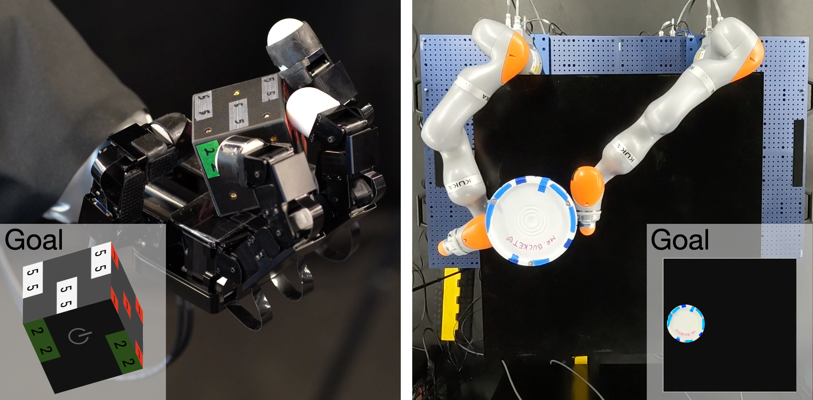
Figure 1: Hardware experiments illustrating the utility of our proposed method in contact-rich manipulation. Left: Dexterous in-hand manipulation with the Allegro hand moving a cube. Right: Whole-body manipulation with bimanual iiwas moving a bucket.

The apparent discrepancy between these two approaches raises the question of how they are related. In fact, analytically deriving the gradients from differentiable simulators shows that the Taylor expansions they produce and the complementarity constraints ubiquitous in contact-implicit trajectory optimization are fundamentally connected (Pang et al., 2023, Example 5). However, the form of each approximation hides a deeper question: where can we trust this local model? In optimization, this region is known as the trust region (Sorensen, 1982). Intuitively, the trust region describes where the local model closely approximates the original function, making it reliable for local improvements. As the quality of Taylor approximations typically degrades as we move further from the nominal point, previous works have often employed an ellipsoidal trust region (Sorensen, 1982; Nocedal and Wright, 2006; More, 1993).

Our first contribution (Section 3) is to elucidate the inconsistency between the ellipsoidal trust region and the unilateral nature of contact. We then address this issue by examining the structure of modern differentiable simulators and proposing the contact trust region (CTR). By augmenting Taylor expansions from these simulators explicitly with feasibility constraints from contact-implicit trajectory optimization, the CTR correctly characterizes the local region in which the Taylor expansions approximate the true contact dynamics well. Not only does CTR connect the Taylor expansions to classical concepts such as the wrench set, it can also be readily derived by combining standard components of existing differentiable simulators.

In this work, we develop CTR based on the quasidynamic differentiable simulator proposed in Pang et al. (2023), called the Convex Quasidynamic Differentiable Contact (CQDC) contact model. The approach could be extended to other contact dynamics models. The CQDC model, recapped in Section 2, is very representative of approaches taken by modern differentiable simulators through contact (Pang et al., 2023; Howell et al., 2023a; Zhong et al., 2022; Werling et al., 2021). It treats simulation of contact as a convex optimization problem whose primal solution becomes the next state $x_{+}$, and gives gradients by performing sensitivity analysis in convex optimization.

However, while a bulk of previous approaches (Suh et al., 2022b; Pang et al., 2023; Howell et al., 2023b; Kurtz and Lin, 2022) have only focused on building a Taylor approximation of the configurations based on sensitivity gradients, our CTR also builds a linear model over the contact forces by utilizing sensitivity analysis to obtain gradients with respect to dual variables. A linear model over the contact forces can further qualify the ellipsoidal trust region by imposing friction cone constraints which are often present in works that directly encode contact complementarity constraints.

The CTR and its connection to convex formulations of contact dynamics also allows us to seamlessly integrate the advances in contact smoothing for planning and control (Howell et al., 2023a; Suh et al., 2022b; Pang et al., 2023; Posa et al., 2014; Onol et al., 2019). Without contact smoothing, many classical methods as well as local trajectory optimizers are limited to fixed contact-mode sequences. Thus, their ability to describe contact mechanics locally has been limited to the relationship between possible contact forces and changes in state within a contact mode. The myopicness of this local model is inconsistent with the non-smooth nature of contact, which also spells trouble for gradient-based Taylor approximations of contact dynamics.

While complementarity-based representations (Aydinoglu et al., 2022) and mixed-integer formulations (Marcucci et al., 2017; Marcucci and Tedrake, 2019; Marcucci et al., 2024; Graesdal et al., 2024) attempt to alleviate this limitation by considering contact mode changes globally, optimizing through these models often require searching through all possible contact-mode sequences. Given the near-exponential scalability of contact modes (Huang et al., 2020), these methods have struggled to tackle problems that are rich in contact. Thus, many successful algorithms go through an approximate representation in which complementarity is omitted in practice (Aydinoglu and Posa, 2022; Todorov, 2014; Jin, 2024).

To alleviate these limitations, smoothing-based methods relax contact dynamics by reasoning about the average result of all the contact modes around a nominal state given some distribution of state and action disturbances. Recent works (Suh et al., 2022b, a) have attributed the success and scalability of Reinforcement Learning (RL) to this mechanism. Surprisingly, however, Pang et al. (2023); Zhang et al. (2023); Howell et al. (2023a) show that for contact dynamics simulated by convex optimization, this process can be done without Monte-Carlo by using barrier smoothing which performs interior-point relaxation of the original contact dynamics and produces force from a distance. However, despite occasional successes, naively applying classical control methods such as LQR on smoothed linearization of contact dynamics often leads to catastrophic failures (Shirai et al., 2024a).

CTR advances the discussion on smoothing by indicating where the smoothed dynamics remain reliable. As our approach draws directly on convex optimization concepts, particularly the sensitivity analysis of primal and dual solutions, we can enjoy the same smoothing benefits by applying an interior-point relaxation that perturbs the original problem’s Karush-Kuhn-Tucker (KKT) optimality conditions.

As our second contribution, we present a highly efficient, contact-implicit Model Predictive Control (MPC) method (Le Cleac’h et al., 2024; Aydinoglu and Posa, 2022) in Section 4. Specialized for contact-rich manipulation, it can be viewed as a natural extension of iterative LQR (Li and Todorov, 2004): we leverage Taylor expansions from CQDC dynamics as linear dynamics constraints, and we include the CTR as additional constraints to capture local contact dynamics. By formulating the CTR as a convex set—specifically, an intersection of multiple second-order cone constraints—each iteration of the proposed MPC remains a convex optimization problem.

We show the efficacy of the proposed CTR and MPC method on two representative contact-rich manipulation problems in Figure 1: i) whole-body manipulation on the bimanual iiwa and cylinder system, and ii) in-hand reorientation on the Allegro hand and cube system. For both systems, we aim to answer the following two questions: i) is the MPC method successful in planning for goals under quasidynamic equations of motion (Section 5), and ii) can the MPC method successfully stabilize quasidynamic plans under true second-order dynamics (Section 6)? Through $2000$ trajectory runs in simulation and $100$ runs on hardware, our results delve into the efficacy and the limitations of our approach, as well as the benefits of CTR over the ellipsoidal one in the context of planning and control.

While our MPC is highly effective in local planning, the goals it can achieve are fundamentally limited by local reachability. For further goals that require non-trivial exploration, its capacity is limited in the absence of a good initial guess. Furthermore, when the MPC encounters such goals, its performance is relatively hard to characterize.

As our final contribution, we address global planning by chaining local trajectories discovered by MPC. To do this, we follow a roadmap (Kavraki et al., 1996) approach where we seed each node with a stable object configuration. Then, we connect these nodes by first finding good actuator configurations for local MPC to start from using CTR (Section 7), then rolling out the MPC plan. To demonstrate the constructed roadmap’s robustness, we perform on the Allegro hand system $150$ consecutive edge traversals before the hardware shuts down due to overheating. For new goals that are not in the roadmap, we simply find the closest node to the goal, then connect them by the same process of finding a good initial actuator configuration and then rolling out MPC.

Our proposed global planning method (Section 8) enables efficient dexterous re-orientation on the Allegro hand, and has several advantages compared to existing approaches. Compared to single-query algorithms (Cheng et al., 2022, 2024; Pang et al., 2023; Khandate et al., 2024), most of the computation time for our algorithm happens offline in the roadmap-building stage, enabling fast online inference. Moreover, the offline roadmap construction only takes minutes on a standard laptop, which is orders-of-magnitude less than approaches based on deep RL(OpenAI et al., 2019; Chen et al., 2022; Handa et al., 2022).

Through our three contributions of i) the contact trust region that approximates contact mechanics efficiently, ii) a highly effective gradient-based MPC controller specialized to local contact-rich manipulation, and iii) a global planner that stitches together local trajectories, our method succeeds in dramatically reducing computation time compared to state-of-the-art methods in RL (OpenAI et al., 2019; Chen et al., 2022; Handa et al., 2022) or sampling-based MPC methods (Howell et al., 2022; Li et al., 2024) without the need for parallelization. We hope digging deep into the structure of contact mechanics can bring efficiency to the current state-of-the-art approaches for whole-body manipulation and dexterous in-hand reorientation.

2 Contact Dynamics as Convex Optimization

Many state-of-art methods for simulating contact solve a constrained optimization problem at every step (Stewart and Trinkle, 2000; Anitescu, 2006; Todorov et al., 2012; Pang and Tedrake, 2021; Howell et al., 2023a; Han et al., 2023; Pang et al., 2023). In this paper, we use the quasi-dynamic formulation of contact dynamics presented in (Pang et al., 2023), where we assume the system is highly damped by frictional forces.

2.1 Setup & Notation

We assume the state consists of configurations, which we denote by $q\in\mathbb{R}^{n_{q}}$, and omit velocities due to the quasi-dynamic assumption. These configurations are divided into actuated configurations ${q^{\mathrm{a}}}\in\mathbb{R}^{n_{q_{\mathrm{a}}}}$ that belong to the robot, and object configurations ${q^{\mathrm{o}}}\in\mathbb{R}^{{n_{q_{\mathrm{o}}}}}$ which are unactuated. Furthermore, the actions are represented as a position command $u\in\mathbb{R}^{n_{q_{\mathrm{a}}}}$ to a stiffness controller with a diagonal gain matrix $\mathbf{K}_{\mathrm{a}}\in\mathbb{R}^{n_{q_{\mathrm{a}}}\times n_{q_{\mathrm{a}}}}$.

2.2 Equations of Motion

At a configuration $q$, the equations of motion are framed as a search for next configurations $q_{\texttt{+}}=({q^{\mathrm{a}}_{\texttt{+}}},{q^{\mathrm{o}}_{\texttt{+}}})$ such that the following force balance equations holds,

$$\mathbf{K}_{\mathrm{a}}({q^{\mathrm{a}}_{\texttt{+}}}-u) =\tau^{\mathrm{a}}+\sum^{n_{c}}_{i=1}(\mathbf{J}_{\mathrm{a}_{i}}(q))^{\top}\lambda_{i}$$ (1a)

$$\epsilon\mathbf{M}_{\mathrm{o}}(q)\frac{{q^{\mathrm{o}}_{\texttt{+}}}-{q^{\mathrm{o}}}}{h^{2}} =\tau^{\mathrm{o}}+\sum^{n_{c}}_{i=1}(\mathbf{J}_{\mathrm{o}_{i}}(q))^{\top}\lambda_{i}$$ (1b)

where $h\in\mathbb{R}_{>0}$ is the timestep, $\tau^{\mathrm{a}}\in\mathbb{R}^{n_{q_{\mathrm{a}}}}$ and $\tau^{\mathrm{o}}\in\mathbb{R}^{{n_{q_{\mathrm{o}}}}}$ are external torques acting on actuated and unactuated bodies respectively (e.g. gravity), and $\epsilon\in\mathbb{R}_{\geq 0}$ is a regularization constant.

In addition, we define an index set $\mathcal{I}_{c}$ over pairs of contact geometries, which we can obtain from a collision detection algorithm. For each contact pair $i\in\mathcal{I}_{c}$, $\lambda_{i}\in\mathbb{R}^{3}$ corresponds to the average contact force over the timestep $h$ at contact $i$, so that $h\lambda_{i}$ is the net impulse generated at contact $i$ during the timestep. By convention, we denote $\lambda_{i}=(\lambda_{\mathrm{n}_{i}},\lambda_{\mathrm{t}_{i}}$) where $\lambda_{\mathrm{n}_{i}}\in\mathbb{R}$ corresponds to contact forces along the normal direction of the contact frames, and $\lambda_{\mathrm{t}_{i}}\in\mathbb{R}^{2}$ corresponds to the frictional forces along the tangential planes.

We also define the contact Jacobians $\mathbf{J}_{i}\in\mathbb{R}^{3\times n_{q}}$ as local mappings from the configurations $q$ to the contact frame. The top row corresponds to the normal direction of the contact frame, where as the bottom two rows orthogonally span the tangential plane. The Jacobians can further be decomposed into mappings into actuated and unactuated DOFs,

$$\mathbf{J}_{i}\coloneqq[\mathbf{J}_{\mathrm{o}_{i}},\mathbf{J}_{\mathrm{a}_{i}}]\coloneqq\begin{bmatrix}\mathbf{J}_{\mathrm{n}_{i}}\\ \mathbf{J}_{\mathrm{t}_{i}}\end{bmatrix}\in\mathbb{R}^{3\times n_{q}}.$$ (2)

With this notational setup, (1a) describes that the configuration of the actuated bodies at the next step, ${q^{\mathrm{a}}_{\texttt{+}}}$, will be decided such that the sum of the forces must be balanced by the force experienced by the stiffness controller at the next step. Similarly, (1b) states that the unbalanced forces result in relative displacements of the object. We can write (1) more succinctly as

$$\mathbf{P}(q){q_{\texttt{+}}}+b(q,u)-\sum_{i=1}^{n_{c}}\mathbf{J}(q)^{\top}\lambda_{i}=0,\;\text{where}$$ (3a)

$$\mathbf{P}(q)\coloneqq\begin{bmatrix}\epsilon\mathbf{M}_{\mathrm{o}}(q)/h^{2}&0\\ 0&\mathbf{K}_{\mathrm{a}}\end{bmatrix},$$ (3b)

$$b(q,u)\coloneqq-\begin{bmatrix}\epsilon\mathbf{M}_{\mathrm{o}}(q){q^{\mathrm{o}}}/h^{2}+\tau^{\mathrm{o}}\\ \mathbf{K}_{\mathrm{a}}u+\tau^{\mathrm{a}}\end{bmatrix}.$$ (3c)

2.3 Contact Constraints

Additional constraints further qualify the relationship between the next configurations ${q_{\texttt{+}}}$ and contact forces $\lambda_{i}$: i) non-penetration: next configuration is non-penetrating; ii) friction cone: $\lambda_{i}$ must be inside the friction cone; iii) complementarity: contact cannot be applied from a distance, and the direction of friction opposes the movement (i.e. maximum dissipation).

To impose these constraints, we first define the feasible velocity cone $\mathcal{K}_{i}$, and then introduce its dual cone $\mathcal{K}_{i}^{\star}$, which corresponds to the friction cone:

$$\mathcal{K}_{i} \coloneqq\left\{\nu_{i}=(\nu_{\mathrm{n}_{i}},\nu_{\mathrm{t}_{i}})\in\mathbb{R}^{3}|\nu_{\mathrm{n}_{i}}\geq\mu_{i}\sqrt{\nu_{\mathrm{t}_{i}}^{\top}\nu_{\mathrm{t}_{i}}}\right\},$$ (4a)

$$\mathcal{K}_{i}^{\star} \coloneqq\left\{\lambda_{i}=(\lambda_{\mathrm{n}_{i}},\lambda_{\mathrm{t}_{i}})\in\mathbb{R}^{3}|\mu_{i}\lambda_{\mathrm{n}_{i}}\geq\sqrt{\lambda_{\mathrm{t}_{i}}^{\top}\lambda_{\mathrm{t}_{i}}}\right\}.$$ (4b)

Anistescu’s relaxation (Anitescu, 2006) allows us to write down these contact constraints in a convex manner by introducing a mild non-physical artifact, where sliding in the tangential plane results in separation in the normal direction,

$$\nu_{i}\coloneqq\mathbf{J}_{i}(q)({q_{\texttt{+}}}-q)+[\phi_{i},0,0]^{\top} \in\mathcal{K}_{i},$$ (5a)

$$\lambda_{i} \in\mathcal{K}_{i}^{\star},$$ (5b)

$$\nu_{i}^{\top}\lambda_{i} =0,$$ (5c)

where $\phi_{i}$ is the current signed distance for contact pair $i$.

2.4 Contact Dynamics as Convex Optimization

We can frame the equations of motion with contact as a search for the next configurations ${q_{\texttt{+}}}$ that satisfy the constraints introduced in Section 2.2 and Section 2.3,

$$\mathrm{find}\quad q_{+}$$ (6a)

s.t. $$\eqref{eq:balance_single_equation},\eqref{eq:friction_constraints:primal_feasibility},\eqref{eq:friction_constraints:dual_feasibility},\eqref{eq:friction_constraints:complementary_slackness}.$$ (6b)

Remarkably, this is equivalent to the KKT conditions of the following Second-Order Cone Program (SOCP),

$$\underset{{q_{\texttt{+}}}}{\mathrm{min}.}\;\frac{1}{2}{q_{\texttt{+}}}^{\top}\mathbf{P}(q){q_{\texttt{+}}}+b(q,u)^{\top}{q_{\texttt{+}}},\;\text{subject to}$$ (7a)

$$\qquad\mathbf{J}_{i}(q){q_{\texttt{+}}}+c_{i}(q)\in\mathcal{K}_{i},\;\forall i\in\mathcal{I}_{c},\;\text{where}$$ (7b)

$$c_{i}(q)\coloneqq[\phi_{i}(q),0,0]^{\top}-\mathbf{J}_{i}(q)q.$$ (7c)

where $\mathcal{I}_{c}$ is the index set over potential contact pairs. Note that stationarity (3), primal feasibility (5a), dual feasibility (5b), and complementary slackness (5c) are the KKT conditions of this SOCP. For complementary slackness of SOCPs, we note that we do not impose element-wise slackness: the primal and dual vectors can both be non-zero as long as they are orthogonal (Boyd and Vandenberghe, 2004; Pang et al., 2023).

In dynamical systems and control theory, it is conventional to represent the dynamic system as a map $f$ that takes a state and input then maps it to the next state. As our state only consists of configurations $q$ for quasidynamic systems, we use the following notation for contact dynamics,

$$q_{+}= f(q,u)$$ (8a)

$$= \text{argmin}_{q_{+}}\;\;\frac{1}{2}q_{+}^{\top}\mathbf{P}(q)q_{+}+b(q,u)^{\top}q_{+},$$

$$\text{subject to}\;\;\mathbf{J}_{i}(q)q_{+}+c_{i}(q)\in\mathcal{K}_{i},\forall i\in\mathcal{I}_{c}.$$ (8b)

Due to the quasidynamic assumption, velocity is omitted from the state, which only consists of the system configuration $$q \mathbf{P},b,\mathbf{J}_{i} c_{i} (q,u)$$. We sometimes omit the explicit dependence of , and on when it is clear from context.

2.5 Smoothing of Contact Dynamics

Despite being continuous and piecewise smooth, the contact dynamics map (8) is well known to have discontinuous gradients (Posa et al., 2014), complicating the application of planning and control methods that rely on local smooth approximations. More specifically, gradient-based methods can be destabilized by fast-changing gradients induced by quickly switching between smooth pieces of the contact dynamics (also called contact modes) (Suh et al., 2022b). In addition, the gradient landscape can have flat regions if none of the contact modes are active, leaving optimizers stranded without informative directions of improvement (Suh et al., 2022a). As such, various dynamic smoothing methods have been proposed to relax this numerical difficulty (Howell et al., 2023a; Pang et al., 2023; Suh et al., 2022b; Posa et al., 2014; Onol et al., 2019; Le Lidec et al., 2024).

In Howell et al. (2023a); Pang et al. (2023), a method of smoothing out optimization-based dynamics was introduced based on the log-barrier (interior-point) relaxation of (7), which solves for the KKT equations where the complementarity condition is perturbed by a positive constant $\kappa$ ,

$$\lambda_{\kappa,i}^{\top}\nu_{i}=2\kappa^{-1}.$$ (9)

The resulting solution is equivalent to solving the log-barrier relaxation of $\eqref{eq:q_dynamic_socp}$,

$$\min_{q_{+}}\;\frac{1}{2}q_{+}^{\top}\mathbf{P}q_{+}+b^{\top}q_{+}-\frac{1}{\kappa}\sum^{n_{c}}_{i=1}\log\left(\nu_{\mathrm{n}_{i}}^{2}/\mu_{i}^{2}-\|\nu_{\mathrm{t}_{i}}\|^{2}\right),$$ (10)

where $\nu_{i}=\mathbf{J}_{i}q_{+}+c_{i}$, and $\nu_{i}=(\nu_{\mathrm{n}_{i}},\nu_{\mathrm{t}_{i}})$ with $\nu_{\mathrm{n}_{i}}\in\mathbb{R}$ and $\nu_{\mathrm{t}_{i}}\in\mathbb{R}^{2}$. The resulting dynamics creates a force-field effect where bodies that are not in contact apply forces inversely proportional to their distance (9).

As the optimization (10) is an unconstrained convex program, its optimality conditions can be obtained by simply setting the gradient of the cost function w.r.t. $q_{+}$ to $0$:

$$\mathbf{P}q_{+}+b-\sum_{i=1}^{n_{\mathrm{c}}}\frac{2\kappa^{-1}}{\nu_{\mathrm{n}_{i}}^{2}/\mu_{i}^{2}-\|\nu_{\mathrm{t}_{i}}\|^{2}}\mathbf{J}_{i}^{\top}\begin{bmatrix}\nu_{\mathrm{n}_{i}}/\mu_{i}^{2}\\ -\nu_{\mathrm{t}_{i}}\\ \end{bmatrix}=0.$$ (11)

As an unconstrained optimization problem, (10) technically does not have dual variables. However, if we consider solving the SOCP dynamics (7) with the interior point method, (10) corresponds to one major iteration along the central path (Boyd and Vandenberghe, 2004, §11.6). Therefore, we can identify average contact forces with the dual feasible points of (7) along the central path:

$$\lambda_{\kappa,i}=\frac{2\kappa^{-1}}{\nu_{\mathrm{n}_{i}}^{2}/\mu_{i}^{2}-\|\nu_{\mathrm{t}_{i}}\|^{2}}\begin{bmatrix}\nu_{\mathrm{n}_{i}}/\mu_{i}^{2}\\ -\nu_{\mathrm{t}_{i}}\end{bmatrix}.$$ (12)

We note that this force i) has a direction opposing the movement in the tangential plane, ii) has a magnitude that satisfies (9), and iii) lies in the friction cone. In addition, plugging (12) into (11) yields

$$\mathbf{P}q_{+}+b-\sum_{i=1}^{n_{c}}\mathbf{J}_{i}^{\top}\lambda_{\kappa,i}=0,$$ (13)

which is equivalent to the force balance equation (3).

Similar to (8), we denote the dynamics map over the relaxed contact dynamics throughout the manuscript as

$$q_{+} =f_{\kappa}(q,u)$$ (14a)

$$=\text{argmin}_{q_{+}}\Big{(}\frac{1}{2}q^{\top}_{+}\mathbf{P}q_{+}+b^{\top}q_{+}$$

$$\quad\quad\quad\quad\quad-\frac{1}{\kappa}\sum^{n_{c}}_{i=1}\log\left(\nu^{2}_{\mathrm{n}_{i}}/\mu_{i}^{2}-\|\nu_{\mathrm{t}_{i}}\|^{2}\right)\Big{)}.$$ (14b)

2.6 Sensitivity Analysis of Smoothed Contact Dynamics

The dynamics map (14) can be interpreted as a solution map from the change in the state and input pair $(q,u)$ to the optimal solutions of the optimization program (10). As various first-order methods in numerical optimization and optimal control often utilize the gradients of the dynamics map $f$ with respect to $q$ and $u$, we detail the computation of these gradients in this section.

The gradients can be computed through sensitivity analysis, which states that as we locally perturb the problem parameters, the solution of (14) change in a way that preserves (up to first-order) the optimality conditions of (14). This is equivalent to stating that the derivative of the equality constraints with respect to $q$ and $u$ are also zero at optimality. For instance, rewriting the derivative of (13) and (9) in matrix form ($\nu_{i}$ and $c_{i}$ need to be expanded using their definitions in (5a) and (7c), respectively) gives

$$\begin{bmatrix}\mathbf{P}&\mathcal{H}_{i}\left[-\mathbf{J}_{i}^{\top}\right]\\ \mathcal{V}_{i}\left[\lambda^{\top}_{i}\mathbf{J}_{i}\right]&\mathcal{D}_{i}\left[\left(\mathbf{J}_{i}q_{+}+c_{i}\right)^{\top}\right]\end{bmatrix}\begin{bmatrix}\frac{\partial{q_{+}}}{\partial{u}}\\ \mathcal{V}_{i}\left[\frac{\partial{\lambda_{\kappa,i}}}{\partial{u}}\right]\end{bmatrix}=\begin{bmatrix}-\frac{\partial{b}}{\partial{u}}\\ 0\end{bmatrix}$$ (15)

where $\mathcal{H}_{i},\mathcal{V}_{i},\mathcal{D}_{i}$ stands for horizontal, vertical, and diagonal stacking of the terms from all contact pairs. Then, we can use the implicit function theorem to solve the system of equations and obtain the derivatives $\partial q_{+}/\partial u$ and $\partial\lambda_{i}/\partial u$ (more details in Section A.1). The derivatives with respect to $q$ may be obtained in a similar fashion, but are more involved due to the $\partial\mathbf{J}_{i}/\partial q$ term (curvature).

3 Local Approximation of Contact Dynamics

Consider a simple, single-horizon optimization problem that involves the contact dynamics (7) as a constraint,

$$\min_{q_{+},u}\quad \|q_{\mathrm{goal}}-q_{+}\|^{2}$$ (16a)

s.t. $$q_{+}=f(q,u).$$ (16b)

A majority of first-order algorithms for optimization and optimal control rely on iteratively making a local approximation of the problem that is more amenable for computation. For instance, gradient-descent makes a linear approximation, and Newton’s method makes a quadratic one. However, we rarely handle the case where the constraint itself is the result of an optimization. In this section, we answer the question: what is the right local approximation of the contact dynamics that i) is computationally convenient, and ii) captures the correct local behavior?

3.1 Linear Model over Smoothed Primal and Dual Variables

Previous works on smooth dynamical systems have often resorted to a first-order Taylor approximation of the dynamics around some nominal coordinates $(\bar{q},\bar{u})$, and approximate the dynamics with a linear model. This Taylor approximation can be compactly written as

$$\hat{q}_{+} =\mathbf{A}\delta q+\mathbf{B}\delta u+f(\bar{q},\bar{u}),$$ (17a)

$$\mathbf{A} \coloneqq\partial f/\partial q(\bar{q},\bar{u}),\;\;\mathbf{B}\coloneqq\partial f/\partial u(\bar{q},\bar{u}),$$ (17b)

$$\delta q \coloneqq q-\bar{q},\;\;\delta u\coloneqq u-\bar{u}.$$ (17c)

However, many previous works (Suh et al., 2022a; Howell et al., 2023a; Pang et al., 2023; Shirai et al., 2024b; Posa et al., 2014) have noted that due to the non-smooth nature of contact, it is beneficial to smooth the dynamics where a first-order Taylor approximation would be valid beyond the contact mode to which $(\bar{q},\bar{u})$ belongs (Pang et al., 2023). A first-order Taylor expansion under such a smoothed dynamics model can be written as

$$\hat{q}_{+} =\mathbf{A}_{\kappa}\delta q+\mathbf{B}_{\kappa}\delta u+f_{\kappa}(\bar{q},\bar{u}),$$ (18a)

$$\mathbf{A}_{\kappa} \coloneqq\partial f_{\kappa}/\partial q(\bar{q},\bar{u}),\;\;\mathbf{B}_{\kappa}\coloneqq\partial f_{\kappa}/\partial u(\bar{q},\bar{u}),$$ (18b)

$$\delta q \coloneqq q-\bar{q},\;\;\delta u\coloneqq u-\bar{u}.$$ (18c)

where $\kappa$ is the barrier smoothing parameter introduced in (9).

Still, as this linear model only gives a local approximation, we would naturally expect the quality of this approximation to degrade as we get further from the nominal coordinates $(\bar{q},\bar{u})$. In order to more rigorously characterize the validity of the local linear model, we need to analyze the behavior of $(q_{+},\lambda_{+,i})$ as we vary $(\delta q,\delta u)$, where $\lambda_{+,i}$ are the linearized dual variables defined by:

$$\hat{\lambda}_{+,i} =\mathbf{C}_{\kappa,i}\delta q+\mathbf{D}_{\kappa,i}\delta u+\lambda_{\kappa,i}(\bar{q},\bar{u}),$$ (19a)

$$\mathbf{C}_{\kappa,i} \coloneqq\partial\lambda_{\kappa,i}/\partial q(\bar{q},\bar{u}),\;\;\mathbf{D}_{\kappa,i}\coloneqq\partial\lambda_{\kappa,i}/\partial u(\bar{q},\bar{u}).$$ (19b)

Lemma 1 (Taylor Approximation).

Consider the joint linear model of the primal and dual variables,

$$\begin{bmatrix}\hat{q}_{+}\\ \mathcal{V}_{i}[\hat{\lambda}_{+,i}]\end{bmatrix}=\begin{bmatrix}\mathbf{A}_{\kappa}&\mathbf{B}_{\kappa}\\ \mathcal{V}_{i}[\mathbf{C}_{\kappa,i}]&\mathcal{V}_{i}[\mathbf{D}_{\kappa,i}]\end{bmatrix}\begin{bmatrix}\delta q\\ \delta u\end{bmatrix}+\begin{bmatrix}f_{\kappa}(\bar{q},\bar{u})\\ \mathcal{V}_{i}[\lambda_{\kappa,i}(\bar{q},\bar{u})]\end{bmatrix}.$$ (20)

Then, this linear model satisfies (13) and (9), the optimality conditions of the perturbed SOCP (10), to first order:

$$\begin{bmatrix}\hat{\mathbf{P}}\hat{q}_{+}+\hat{b}-\sum^{n_{c}}_{i=1}\hat{\mathbf{J}}_{i}^{\top}\hat{\lambda}_{+,i}\\ \mathcal{V}_{i}\left[(\hat{\mathbf{J}}_{i}\hat{q}_{+}+\hat{c}_{i})^{\top}\hat{\lambda}_{+,i}-2\kappa^{-1}\right]\end{bmatrix}=\mathcal{O}\left((\delta q,\delta u)^{2}\right)$$ (21)

with $\hat{\mathbf{P}}\coloneqq\mathbf{P}(\bar{q},\bar{u})+\frac{\partial\mathbf{P}}{\partial q}\delta q+\frac{\partial\mathbf{P}}{\partial u}\delta u$, and similarly for $\hat{b}$, $\hat{\mathbf{J}}$, and $\hat{c}_{i}$.

Proof.

If we expand the Taylor-approximated equations and drop the terms above first-order, we are left with i) the original equality conditions over nominal coordinates which must hold due to the nominal values being obtained at optimality and ii) its first-order expansion, which must hold due to the definition of the sensitivity gradients (15). ∎

3.2 Ellipsoidal Trust Region (ETR)

Lemma 1 implies that the linear model will no longer be accurate far away from $(\bar{q},\bar{u})$, even with the benefits of smoothing (Pang et al., 2023). As such, many optimization methods are further concerned with where we can trust the local model, and introduce the concept of a trust region around ($\bar{q},\bar{u})$, which further qualifies the accuracy of the linear model (Sorensen, 1982; More, 1993). To simplify computation, these trust regions are often chosen to be simple geometric primitives.

Following classical works, let us first consider an ellipsoidal trust region which can be described in quadratic form:

$$\mathcal{E}_{\mathbf{\Sigma}}(\bar{q},\bar{u})\coloneqq\{\delta z=(\delta q,\delta u)|\delta z^{\top}\mathbf{\Sigma}\delta z\leq 1\}.$$ (22)

The set of ${q}_{+}$ achievable with this ellipsoidal trust region can be written as

$$\{\hat{q}_{+}|\hat{q}_{+}=\mathbf{A}_{\kappa}\delta q+\mathbf{B}_{\kappa}\delta u+f_{\kappa}(\bar{q},\bar{u}),(\delta q,\delta u)\in\mathcal{E}_{\mathbf{\Sigma}}(\bar{q},\bar{u})\}$$ (23)

We emphasize the set (23) is still an ellipsoid, as it is the image of the ellipsoid $\mathcal{E}_{\mathbf{\Sigma}}(\bar{q},\bar{u})$ under the linear map $(\mathbf{A}_{\kappa},\mathbf{B}_{\kappa})$ with a constant offset $f_{\kappa}(\bar{q},\bar{u})$.

In order for this linear model to be consistent with the true dynamics within the trust region, choosing an appropriate trust region parameter $\mathbf{\Sigma}$ is imperative. If $\mathbf{\Sigma}$ has too large of a volume, it is likely that there will be large errors in the behavior of the system within the trust region. On the other hand, if $\mathbf{\Sigma}$ is too small, iterative algorithms will have to take more iterations to converge.

3.3 Contact Trust Region (CTR)

However, contact is more special in that it is a unilaterally constrained dynamical system. If points in the trust region predicts a behavior of primal and dual variables that are not feasible, this can also cause a large discrepancy in the approximated model within the trust region. In practice solvers would also try to find an ellipsoidal trust region such that all the elements within the trust region would result in a feasible prediction (Moré and Sorensen, 1983; Niu and Yuan, 2010). However, this is often achieved by shrinking the ETR centered at the linearization point, resulting in overly conservative(small) trust regions.

Thus, we propose to separate the role of the ellipsoid in keeping Taylor approximation error low, and having to be inscribed within the feasible set. This is achievable by intersecting the ellipsoidal trust region and the primal and dual feasible set of the SOCP contact dynamics (7) under linearized approximations of the primal and dual variables. We formalize this object in Definition 1.

Definition 1 (Contact Trust Region).

We define the Contact Trust Region (CTR) at $(\bar{q},\bar{u})$ as the set of all allowable perturbations that do not result in violation of the primal and dual feasibility constraints under a linear model,

$$\mathcal{S}_{\mathbf{\Sigma},\kappa}(\bar{q},\bar{u})\coloneqq\{ (\delta q,\delta u)|\delta z^{\top}\mathbf{\Sigma}\delta z\leq 1,\delta z=(\delta q,\delta u),$$ (24a)

$$\hat{q}_{+} =\mathbf{A}_{\kappa}\delta q+\mathbf{B}_{\kappa}\delta u+f_{\kappa}(\bar{q},\bar{u}),$$ (24b)

$$\hat{\lambda}_{+,i} =\mathbf{C}_{\kappa,i}\delta q+\mathbf{D}_{\kappa,i}\delta u+\lambda_{\kappa,i}(\bar{q},\bar{u}),$$ (24c)

$$\hat{\mathbf{J}}_{i}\hat{q}_{+}+\hat{c}_{i} \in\mathcal{K}_{i},$$ (24d)

$$\hat{\lambda}_{+,i} \in\mathcal{K}^{\star}_{i}\}.$$ (24e)

Although the linearizations (24b) and (24c) are taken under the smoothed, unconstrained dynamics (10), enforcing the feasibility constraints of the SOCP dynamics (7) is still justified. Firstly, the primal feasibility constraint (24d) is implied by the domain of the logarithm in (10). Furthermore, although the nominal contact forces $\lambda_{\kappa,i}$ in are dual feasible (because of (12)), we still need to ensure the feasibility of the linearization $\hat{\lambda}_{\kappa,i}$ by including (24e).

Oftentimes we are also interested in the effect of action perturbations for a fixed nominal state. Therefore, we introduce a simplified case of the CTR that has zero perturbations in configuration $(\delta q=0)$.

Definition 2 (Action-only Contact Trust Region).

We define the Action-only Contact Trust Region (A-CTR) as

$$\mathcal{S}^{\mathcal{A}}_{\mathbf{\Sigma},\kappa}(\bar{q},\bar{u})\coloneqq\{\delta u| \delta u^{\top}\mathbf{\Sigma}\delta u\leq 1,$$ (25a)

$$\hat{q}_{+} =\mathbf{B}_{\kappa}\delta u+f_{\kappa}(\bar{q},\bar{u}),$$ (25b)

$$\hat{\lambda}_{+,i} =\mathbf{D}_{\kappa,i}\delta u+\lambda_{\kappa,i}(\bar{q},\bar{u}),$$ (25c)

$$\mathbf{J}_{i}\hat{q}_{+}+c_{i} \in\mathcal{K}_{i},$$ (25d)

$$\hat{\lambda}_{+,i} \in\mathcal{K}^{\star}_{i}\}.$$ (25e)

Both the CTR (24) and the A-CTR (25) are convex as they each can be expressed as an intersection of convex constraints.

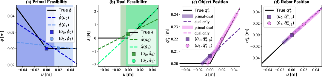
Figure 2: A-CTR illustrations for the system in Figure 3b at $(\bar{q}^{\mathrm{o}},\bar{q}^{\mathrm{a}})=(0.2,0)$. Sub-figures show how (a) the signed distance function $\phi$, (b) the contact force $\lambda$, (c) the object configuration ${q^{\mathrm{o}}_{\texttt{+}}}$ and (d) the robot configuration ${q^{\mathrm{a}}_{\texttt{+}}}$ change as a function of the action $u$. In every sub-figure, the black solid line represents the true, non-smooth dynamics (8). The markers (squares and circles) represent linearization points. In (a) and (b), the deeper-colored dotted lines represent the linearization at $\bar{u}_{0}=0$, and the lighter-colored lines represent the linearization at $\bar{u}_{1}=0.02$. The shaded regions represent the feasible set of the corresponding color. For instance, the dark blue shaded region in (a) represents $\hat{\phi}\left(\bar{q}=(0.2,0),\bar{u}=0\right)\geq 0$; the light green region in (b) represents $\hat{\lambda}_{+}\left(\bar{q}=(0.2,0),\bar{u}=0.02\right)\geq 0$. In (c) and (d), the dotted lines show parts of the linearizations that satisfy only the dual constraints; the thick shaded lines around dotted lines satisfy both the primal and dual constraints.

Example 1 (A-CTR for 1D Pushing).

Consider the 1D system in Figure 3 with two bodies of width $0.2\mathrm{m}$, one actuated (red sphere) and one unactuated (gray box), both constrained to slide on a frictionless surface along the $x$ axis.

In this example, we illustrate the A-CTRs for the nominal configuration in Figure 3b, where $\bar{q}=(\bar{q}^{\mathrm{o}},\bar{q}^{\mathrm{a}})=(0.2,0)$: the ball is touching the left face of the box.

Firstly, we note that the true, non-smooth contact dynamics (defined by (8) and shown as the black line segments in Figure 2a-c) has two contact modes: (i) a no-contact mode corresponding to the left linear piece with domain $u\leq 0$, and (ii) an in-contact mode corresponding to the right piece with domain $u\geq 0$. The two modes are also present in the robot dynamics in Figure 2d, but the slope difference between the two modes is barely noticeable.

Secondly, the dual feasibility constraints (25e) are crucial to prevent unphysical behaviors, such as pulling the object via contact forces. As shown in Figure 2b, the linearizations (dotted lines) incorrectly suggest the box can pull the object with a negative $u$. However, once the system switches to no-contact mode according to the true dynamics, the box remains stationary. By enforcing dual feasibility on $\hat{\lambda}$, the vast majority of negative $u$ is restricted, as demonstrated by the green shaded regions in Figure 2b. A small amount of negative $u$ is still allowed due to mismatch between the gradients of the smoothed and true dynamics.

Interestingly, we observe that although the smoothed gradient does not perfectly match the gradient of the true dynamics, the mismatch can be reduced by tweaking the linearization point. As shown in Figure 2, the linearization at $\bar{u}_{0}=0.0$ under smoothed contact dynamics does not match the gradient of either mode well, as $\bar{u}_{0}$ is on the boundary between the two modes. As a result, the boundary of the feasible regions computed from the linearization (e.g. dark green shaded region in Figure 2b) does not match the boundary of the in-contact mode perfectly. On the other hand, for $\bar{u}_{1}=0.02$, a linearization point further away from the boundary of the domain of the in-contact mode, both the linearization (light green dotted line) and the approximated boundary of the dual feasible set (light green shaded region) match the in-contact piece much more closely.

Lastly, we argue that enforcing the primal feasibility constraint (25d) can needlessly restrict robot motion. As shown in Figure 2a, under the true signed-distance function, the entire in-contact piece satisfies the non-penetration constraint with $\phi=0$. However, due to the slight gradient mismatch introduced by smoothing, the linear approximation $\hat{\phi}$ is never perfectly flat. Consequently, the primal-dual feasible regions (shaded regions in Figure 2c and Figure 2d) end just a few centimeters ahead of the linearization points, whereas the linear approximations alone remain valid over a much larger domain defined solely by the dual constraints (dashed lines in the same sub-figures).

However, imposing the primal and dual feasibility constraints in (24) does not always reduce the trust region size, which we illustrate in Example 2.

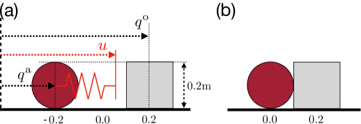
Figure 3: (a) Schematic of the 1-dimensional pusher system used in Example 1. (b) corresponds to the configuration $({q^{\mathrm{o}}},{q^{\mathrm{a}}})=(0.2,0)$.

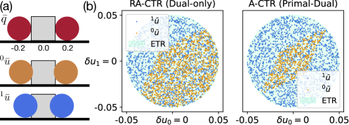
Figure 4: (a) Nominal configuration and actions for Example 2. $u_{0}$ and $u_{1}$ are the position commands of the left and right ball, respectively. (b) Samples in the action space that satisfy the primal (24d) and dual (24e) feasibility constraints for different nominal actions.

Example 2 (A-CTR for 1D Squeezing).

Consider the 1D system in Figure 4. Similar to Example 1, both the robot and the object slide on a frictionless surface. But the robot now consists of two actuated spheres, one on each slide of the box. We illustrate the A-CTRs for the nominal configuration in Figure 4a, where $\bar{q}^{\mathrm{o}}=0.0$ and $\bar{q}^{\mathrm{a}}=(-0.2,0.2)$: each side of the box has a ball touching it. The action space for this system is 2D. In the ETR constraint (24a), we set $\mathbf{\Sigma}=\mathrm{diag}([0.05^{2},0.05^{2}])^{-1}$, i.e. the ETR is a sphere of radius $0.05$ (blue spheres in Figure 4b).

We sample 2000 points from the ETR, reject samples that violate the primal and/or dual feasibility constraints, and plot the remaining samples in Figure 4b. For the nominal action ${}^{0}\bar{u}=(-0.19,0.19)$ (orange dots), the feasibility constraints eliminate a fair amount of samples. Enforcing both primal and dual constraints eliminate more samples than enforcing only the dual constraints.

However, as the nominal action gets deeper into penetration, e.g. ${}^{1}\bar{u}=(-0.16,0.16)$ (blue dots), both the primal-dual and the dual-only feasible regions grow and completely contain the ETR, as shown by the blue dots covering the blue spheres entirely in Figure 4b.

This is not a surprising result: as the spheres squeeze the box harder (deeper commanded penetration), there is more room to wiggle the nominal action without losing contact.

3.4 Relaxed Contact Trust Region (R-CTR)

We believe the unnecessary restrictions on trust region sizes caused by the primal feasibility constraint in Example 1 are not an isolated phenomenon, and we hypothesize that imposing primal feasibility in general is too conservative. In particular, under a linear model of the smoothed dynamics, the sensitivity of the actuated bodies is often larger than the sensitivity of unactuated objects: this is a relaxation of the sensitivity of the unactuated body being $\mathbf{0}$ and the actuated body being $\mathbf{I}$ when not in contact. Therefore, the actuated body catches up to penetrate the unactuated object upon very small perturbations.

Accordingly, we define variants of CTR and A-CTR that relax the primal feasibility constraint.

Definition 3 (Relaxed Contact Trust Region).

We define the Relaxed Contact Trust Region (R-CTR) at $(\bar{q},\bar{u})$ as the set of all allowable perturbations that satisfy only the dual feasibility constraints under a linear model,

$$\tilde{\mathcal{S}}_{\mathbf{\Sigma},\kappa}(\bar{q},\bar{u})\coloneqq\{ (\delta q,\delta u)|\delta z^{\top}\mathbf{\Sigma}\delta z\leq 1,\delta z=(\delta q,\delta u),$$ (26a)

$$\hat{q}_{+} =\mathbf{A}_{\kappa}\delta q+\mathbf{B}_{\kappa}\delta u+f_{\kappa}(\bar{q},\bar{u}),$$ (26b)

$$\hat{\lambda}_{+,i} =\mathbf{C}_{\kappa,i}\delta q+\mathbf{D}_{\kappa,i}\delta u+\lambda_{\kappa,i}(\bar{q},\bar{u}),$$ (26c)

$$\hat{\lambda}_{+,i} \in\mathcal{K}^{\star}_{i}\}.$$ (26d)

Definition 4 (Relaxed Action-only Contact Trust Region).

We define the Relaxed Action-only Contact Trust Region (RA-CTR) as

$$\tilde{\mathcal{S}}^{\mathcal{A}}_{\mathbf{\Sigma},\kappa}(\bar{q},\bar{u})\coloneqq\{\delta u| \delta u^{\top}\mathbf{\Sigma}\delta u\leq 1,$$ (27a)

$$\hat{q}_{+} =\mathbf{B}_{\kappa}\delta u+f_{\kappa}(\bar{q},\bar{u}),$$ (27b)

$$\hat{\lambda}_{+,i} =\mathbf{D}_{\kappa,i}\delta u+\lambda_{\kappa,i}(\bar{q},\bar{u}),$$ (27c)

$$\hat{\lambda}_{+,i} \in\mathcal{K}^{\star}_{i}\}.$$ (27d)

In both Definition 3 and Definition 4, we keep $\hat{q}^{\mathrm{a}}$ although they are not directly used in the trust region definitions: they are useful for imposing joint and torque limits, which are detailed in Section 3.6.

Furthermore, we make the following definition for the predicted dynamics over the relaxed trust regions.

Definition 5 (Motion Set).

We define the image of $\tilde{\mathcal{S}}(\bar{q},\bar{u})$ under the linearized primal solution map as the Motion Set,

$$\mathcal{M}_{\mathbf{\Sigma,\kappa}}(\bar{q},\bar{u})\coloneqq\{\hat{q}_{+}| \hat{q}_{+}=\mathbf{A}_{\kappa}\delta q+\mathbf{B}_{\kappa}\delta u+f_{\kappa}(\bar{q},\bar{u}),$$ (28a)

$$(\delta q,\delta u)\in\tilde{\mathcal{S}}_{\mathbf{\Sigma},\kappa}(\bar{q},\bar{u})\}.$$ (28b)

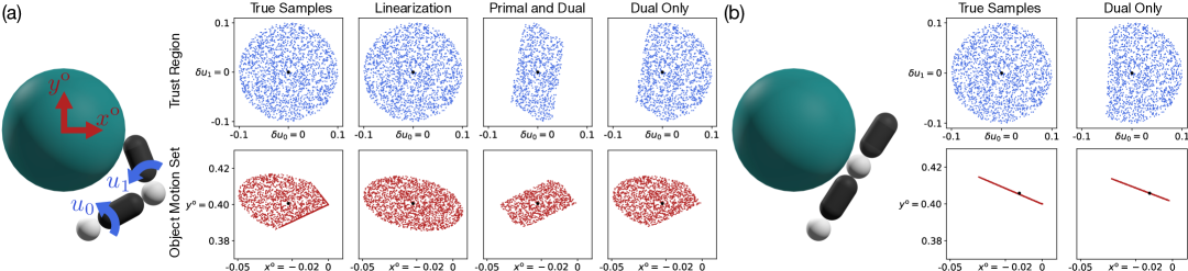
Figure 5: Visualization of the A-CTR $\mathcal{S}^{\mathcal{A}}_{\mathbf{\Sigma},\kappa}$ (primal and dual), RA-CTR $\tilde{\mathcal{S}}^{\mathcal{A}}_{\mathbf{\Sigma},\kappa}$ (dual only) and the action-only object motion set $\mathcal{M}^{\mathcal{A},\mathrm{o}}_{\mathrm{\Sigma},\kappa}$ under the different linearization points shown in the illustrations. In the “Trust Region” row, the “True Samples” subplot is obtained by uniformly sampling 2000 points from the ball $\left\lVert{\delta u}\right\rVert\leq 0.1$; samples in the following columns are obtained by rejecting samples that do not satisfy the respective constraints. In the “Object Motion Set” row, the “True Samples” subplot is obtained by passing the $\delta u$ samples from the trust region subplot above through the true contact dynamics (8); samples in the following columns are obtained by mapping the $\delta u$ samples from the corresponding trust region subplot through the linear map defined in (29).

Definition 6 (Action-only Motion Set).

We define the image of $\tilde{\mathcal{S}}^{\mathcal{A}}_{\Sigma,\kappa}(\bar{q},\bar{u})$ under the linearized primal solution map as the Action-only Motion Set,

$$\mathcal{M}^{\mathcal{A}}_{\mathbf{\Sigma,\kappa}}(\bar{q},\bar{u})\coloneqq\{\hat{q}_{+}| \hat{q}_{+}=\mathbf{B}_{\kappa}\delta u+f_{\kappa}(\bar{q},\bar{u}),$$ (29a)

$$\delta u\in\tilde{\mathcal{S}}^{\mathcal{A}}_{\mathbf{\Sigma},\kappa}(\bar{q},\bar{u})\}.$$ (29b)

Similar to how we partition $q$ into ${q^{\mathrm{o}}}$ and ${q^{\mathrm{a}}}$, we use superscripts $\cdot^{\mathrm{o}}$ and $\cdot^{\mathrm{a}}$ to denote subsets of $\mathcal{M}_{\mathbf{\Sigma,\kappa}}$ corresponding to the object and robot configurations, respectively. For example, $\mathcal{M}^{\mathcal{A},\mathrm{o}}_{\mathbf{\Sigma},\kappa}(\bar{q},\bar{u})\coloneqq\{\hat{q}^{\mathrm{o}}_{+}|\hat{q}_{+}\in\mathcal{M}^{\mathcal{A}}_{\mathbf{\Sigma},\kappa}(\bar{q},\bar{u})\}$. In addition, as a linear map of a convex set, the motion set (28) is also convex.

Example 3 (A-CTRs and Motion Sets).

Consider the simple robotic system in Figure 5, where a 2-joint robot arm attempt to move a sphere which has two translational DOFs $(x^{\mathrm{o}},y^{\mathrm{o}})$ and does not rotate. The motion sets attempt to approximate the 1-step reachable set at the nominal configurations in the figure. Nominal actions are chosen so that the robot is slightly in penetration with the object.

Firstly, the motion set with only the linearization and no feasibility constraints cannot capture the unilateral nature of contact, as ellipsoids are bi-directional.

Secondly, imposing both primal and dual feasibility constraints yields an overly conservative representation of the object’s possible motion. In contrast, enforcing only dual feasibility provides a closer match to the true object motion set. This is consistent with our observations from Example 1.

Lastly, from Figure 5b, we note the proposed action-only motion set, $\mathcal{M}^{\mathcal{A},\mathrm{o}}_{\mathrm{\Sigma},\kappa}$, respects singular robot configurations, as the sensitivity analysis procedure factor in the configuration of the manipulator.

3.5 Mechanics Derivation of the Motion Set

We can further motivate the idea that relaxing the primal feasibility constraints improves local approximations of feasible object motions by connecting the RA-CTR to classical constructs in manipulation, such as the motion cone (Mason, 1986; Chavan-Dafle et al., 2020) and the wrench set (Ferrari and Canny, 1992; Lynch and Park, 2017). In this section, we establish these connections by providing an alternative derivation of the action-only motion set (Definition 6), starting from contact forces instead of Taylor expansions.

The Contact Force Set. For a single contact pair $i$, the predicted linear model of how the contact force changes as we vary $\delta u$ is given by $\hat{\lambda}_{+,i}=\mathbf{D}_{\kappa,i}\delta u+\lambda_{\kappa,i}(\bar{q},\bar{u})$, as long as the prediction $\hat{\lambda}_{+,i}$ lies within the friction cone $\mathcal{K}^{\star}_{i}$. Thus, the set of allowable contact forces for this pair is given by

$$\mathcal{C}^{\mathcal{A}}_{\mathbf{\Sigma},\kappa,i}(\bar{q},\bar{u})\coloneqq\big{\{}\hat{\lambda}_{+,i}| \hat{\lambda}_{+,i}=\mathbf{D}_{\kappa,i}\delta u+\lambda_{\kappa,i}(\bar{q},\bar{u})$$ (30a)

$$\hat{\lambda}_{+,i}\in\mathcal{K}_{i}^{\star},$$ (30b)

$$\delta u^{\top}\mathbf{\Sigma}\delta u\leq 1\big{\}}.$$ (30c)

The Generalized Friction Cone. The generalized friction cone (Erdmann, 1994) is a linear mapping of the friction cone to the space of object wrenches. This can be obtained by applying the contact Jacobian that linearizes the kinematics of the contact point with respect to object coordinates,

$$\mathcal{JC}^{\mathcal{A}}_{\mathbf{\Sigma},\kappa,i}(\bar{q},\bar{u})\coloneqq\left\{w_{i}|w_{i}=\mathbf{J}_{\mathrm{o}_{i}}^{\top}\lambda_{+,i},\;\lambda_{+,i}\in\mathcal{C}^{\mathcal{A}}_{\mathbf{\Sigma},\kappa,i}\right\}.$$ (31a)

The Wrench Set. The wrench set (Ferrari and Canny, 1992; Lynch and Park, 2017) is defined as the set of all achievable wrenches that can be applied to an object given all possible contact forces that can be applied from a given configuration. This quantity has classically served as an important metric in grasping analysis (Ferrari and Canny, 1992; Han et al., 2000; Dai et al., 2016). While the classical wrench set has bounds on the contact force, we instead apply bounds on the actuator input ($\|\delta u\|_{\mathbf{\Sigma}}^{2}\leq 1$).

Our version of the wrench set is defined by taking Minkowski sums of each generalized friction cone $\mathcal{JC}^{\mathcal{A}}_{\mathbf{\Sigma},\kappa,i}$ for all contact pairs,

$$\mathcal{W}^{\mathcal{A}}_{\mathbf{\Sigma},\kappa}(\bar{q},\bar{u})\coloneqq\{w|w =\tau^{\mathrm{o}}+\textstyle\sum_{i}w_{i}$$ (32a)

$$w_{i} \in\mathcal{JC}^{\mathcal{A}}_{\mathbf{\Sigma},\kappa,i}(\bar{q},\bar{u})\},$$ (32b)

where $h\tau^{\mathrm{o}}$ is some external impulse on the object (e.g. by gravity). The wrench set adequately describes the set of all wrenches that can be applied on the object from a given nominal configuration and input $(\bar{q},\bar{u})$.

The Motion Set. The motion set is analogous to motion cones (Mason, 1986; Chavan-Dafle et al., 2020). While classical motion cones describe the set of feasible object velocity under a single patch contact, we define motion cone as the set of all feasible displacements achievable by multiple contacts in one time step.

We construct this object by utilizing a quasistatic relation between the object movement and the applied impulse (1b),

$$\mathcal{M}^{\mathcal{A},\mathrm{o}}_{\mathbf{\Sigma},\kappa}(\bar{q},\bar{u})=\{\hat{q}_{+}^{\mathrm{o}}| \epsilon\mathbf{M}_{\mathrm{o}}(\bar{q})\left(\hat{q}^{\mathrm{o}}_{+}-\bar{q}^{\mathrm{o}}\right)/h=hw,$$ (33a)

$$w\in\mathcal{W}^{\mathcal{A}}_{\mathbf{\Sigma},\kappa}(\bar{q},\bar{u})\}.$$ (33b)

We are now ready to draw the connection between the construction of motion sets in this section, and the definition of the motion set as the image of the trust region in Definition 6.

Lemma 2.

The object motion set derived in (33) is equivalent to object subset of the Action-only Motion Set $\mathcal{M}^{\mathcal{A}}_{\mathbf{\Sigma,\kappa}}(\bar{q},\bar{u})$ defined in Definition 6.

Proof.

Section A.2. ∎

3.6 Additional Constraints

We list some additional constraints and costs that may be added to this formulation to further restrict the CTR.

3.6.1 Joint Limits

Consider joint limits $q^{\mathrm{a}}_{lb}$ and $q^{\mathrm{a}}_{lb}$ that must be enforced by the robot. Then, we can add the constraint that limits the position command that we send to the robot,

$$q^{\mathrm{a}}_{lb}\leq\bar{u}+\delta u\leq q^{\mathrm{a}}_{ub}.$$ (34)

3.6.2 Torque Limits

We often want to limit the torque applied by the robot to the object by imposing lower and upper bounds $\tau_{lb}$ and $\tau_{ub}$ on joint torque. Although the quasi-dynamic formulation cannot account for dynamic transient torques, we can compute the steady-state torque experienced by the robot using the difference in the sent position command and the predicted position (Pang and Tedrake, 2022). Thus, the set of achievable $\delta u$ that does not violate this steady-state torque limit can be written as

$$\tau_{lb}\leq\mathbf{K}_{\mathrm{a}}^{-1}\left(\bar{q}^{\mathrm{a}}_{+}+\mathbf{B}^{\mathrm{a}}\delta u-(\bar{u}+\delta u)\right)\leq\tau_{ub}.$$ (35)

where $\tau^{\mathrm{a}}$ accounts for gravitational torques on the robot.

4 Local Planning and Control

We now study local gradient-based planning and control, which is one of the core applications of our proposed contact trust region. Among possible formulations of this problem, we focus on computing a configuration and input sequence that moves the system towards a goal configuration $q_{\text{goal}}$. The full nonlinear form of this problem can be written as

$$\min_{q_{0:T},u_{0:T-1}}\quad \|q_{\text{goal}}-q_{T}\|^{2}_{\mathbf{Q}}+\sum^{T-1}_{t=0}\|u_{t}-u_{t-1}\|^{2}_{\mathbf{R}},$$ (36a)

s.t. $$q_{t+1}=f(q_{t},u_{t})\quad\forall t,$$ (36b)

$$|u_{t}-u_{t-1}|\leq\eta\quad\forall t,$$ (36c)

$$q_{0}=\bar{q}_{0},$$ (36d)

where (36b) enforces dynamics constraints, (36c) enforces input limits (recall that $u_{t}$ is a position command, thus input limits are enforced in relative form), and (36d) enforces the initial condition.

One of the biggest challenges in solving (36) is handling the non-smooth contact dynamics constraint (36b). Although MIP-based methods (Marcucci et al., 2017; Marcucci and Tedrake, 2019) have struggled to scale up to complex, contact-rich problems, the MIP formulation reveals why the problem is hard: the search through the exponentially many contact modes.

In this section, we present a method for solving (36) by incorporating contact dynamics smoothing and the contact trust region into an iLQR-like (Li and Todorov, 2004) trajectory optimization scheme. Through two toy problems, we show that the proposed method can iteratively approach an advantageous contact mode for reaching the given goals, even when the initial guess is in a contact mode with non-informative gradient. In addition, we present how the method can be used as a model predictive controller and be extended to control contact forces.

4.1 Trajectory Optimization with R-CTR

Consider a trajectory optimization scheme, where we first obtain some guess of the nominal input $\bar{u}_{0:T-1}$, then roll it out under the dynamics to get the nominal configuration trajectory $\bar{q}_{0:T}$. Under a local approximation of (36) around this nominal trajectory $(\bar{q}_{0:T},\bar{u}_{0:T-1})$ utilizing gradients of smoothed dynamics and R-CTR, we search for optimal perturbations $(\delta q_{0:T},\delta u_{0:T-1})$ by solving the following local trajectory optimization problem with linear dynamics constraints:

$$\mathrm{SubTrajOpt}(\bar{q}_{0:T},\bar{u}_{0:T-1},q_{\text{goal}})=\delta u^{\star}_{0:T-1},\text{where}$$ (37a)

$$\min_{\delta q_{0:T},\delta u_{0:T-1}}\quad\|q_{\text{goal}}-q_{T}\|^{2}_{\mathbf{Q}}+\sum^{T-1}_{t=0}\|u_{t}-u_{t-1}\|^{2}_{\mathbf{R}},$$ (37b)

$$\text{s.t.}\quad\delta q_{t+1}=\mathbf{A}_{\kappa,t}\delta q_{t}+\mathbf{B}_{\kappa,t}\delta u_{t},\;t=0\dots T-1,$$ (37c)

$$\quad\quad(\delta q_{t},\delta u_{t})\in\tilde{\mathcal{S}}_{\mathbf{\Sigma,\kappa}}(\bar{q}_{t},\bar{u}_{t}),\;t=0\dots T-1,$$ (37d)

$$\quad\quad q_{t}=\bar{q}_{t}+\delta q_{t},\;t=0\dots T,$$ (37e)

$$\quad\quad u_{t}=\bar{u}_{t}+\delta u_{t},\;t=0\dots T-1,$$ (37f)

$$\quad\quad|u_{t}-u_{t-1}|\leq\eta,\;t=1\dots T-1,$$ (37g)

$$\quad\quad\delta q_{0}=0,$$ (37h)

Here (37c) is the standard linear dynamics constraint in linear MPC, where $\delta q_{t+1}\coloneqq q_{t+1}-f(\bar{q}_{t},\bar{u}_{t})$; $\tilde{\mathcal{S}}_{\mathbf{\Sigma,\kappa}}$ in (37d) is the R-CTR (26); (37c) and (37d) constitute our local approximation of the contact dynamics constraint (36b); (37h) is due to the initial condition constraint (36d). The sub trajectory optimization problem (37) is a standard SOCP that can be solved by off-the-shelf conic solvers. We note that other constraints as joint limits and torque limits in Section 3.6 can be added trivially to this formulation by incorporating them into $\tilde{\mathcal{S}}_{\mathbf{\Sigma},\kappa}$.

After obtaining the optimal values $\delta q_{t}^{\star},\delta u_{t}^{\star}$, we update the nominal input trajectory with $\bar{u}_{t}\leftarrow\bar{u}_{t}+\delta u_{t}^{\star}$, and repeat the process of rolling out to obtain nominal configuration trajectory, and searching for local improvements. This iterative scheme is summarized in Algorithm 1.

Notably, the rollout step (Algorithm 1) is analogous to the forward pass in iLQR; the $\mathbf{SubTrajOpt}$ step (Algorithm 1) is analogous to the backward pass. Unlike iLQR’s backward pass, which solves for the optimal action perturbations $\delta u_{t}$ iteratively using Bellman recursion, $\mathbf{SubTrajOpt}$ solves for all $\delta u_{t}$ jointly with convex optimization.

Lastly, we impose the relaxed CTR constraint in (37d) instead of the full CTR, as the full CTR often leads to under approximation of the 1-step reachable set of the true dynamics. We have shown this via simple examples in Section 3, and will show more experimental support for the choice of using R-CTR in Section 5.

1 Input: Initial state $q_{0}$, goal state $q_{\text{goal}}$, input trajectory guess $\bar{u}_{0:T-1}$, iterations limit $n_{\mathrm{max}}$;

2 Output: Optimized input trajectory $\bar{u}_{0:T-1}^{\star}$;

3 $n\leftarrow 0$;

4 while not converged $\mathrm{and}$ $n<n_{\mathrm{max}}$ do

5    $\bar{q}_{0:T}\leftarrow$ Rollout $f$ from $q_{0}$ with $\bar{u}_{0:T-1}$ ;

6    $\delta u_{0:T-1}^{\star}\leftarrow\mathbf{SubTrajOpt}(\bar{q}_{0:T},\bar{u}_{0:T-1})$ ;

7    $\bar{u}_{t}\leftarrow\bar{u}_{t}+\delta u_{t}^{\star}\quad\forall t$;

8    $n\leftarrow n+1$

return$\;\bar{u}_{0:T-1}$

Algorithm 1 CTR Trajectory Optimization-CtrTrajOpt

4.2 Initial Guess Heuristic

As the trajectory optimization problem (36) is nonconvex, the solution that Algorithm 1 converges to can be sensitive to the choice of initial guesses for the input trajectory $\bar{u}_{0:T-1}$. The most uninformed initial guess would be to set the position command to be the current configuration of actuated bodies ($\bar{u}_{t}=\bar{q}^{\mathrm{a}}_{0},\forall t$). However, this can be problematic especially when the robots are not in contact with the object in $q_{0}$, as $\mathbf{B}_{\kappa}^{\mathrm{u}}$, the gradient of object motion w.r.t. robot actions, can get close to $0$ even with dynamics smoothing when the distance between them are far away.

To alleviate this problem, we can compute a position command that would result in the closest contacting configuration from $q_{0}$, and pass this command as the initial guess for $\bar{u}_{0:T-1}$.

To compute this initial guess, we utilize the intuition that the log-barrier smoothed dynamics in (10) results in a force-from-a-distance like effect that pushes away objects even when not in contact. We simply reverse this force field by sending the following torque to the robot,

$$\tau=-\sum_{i}{\mathbf{J}^{\mathrm{o}}_{i}}^{\top}\lambda_{i}$$ (38)

and simulate forward using Drake (Han et al., 2023) until the robot is in contact with the object.

4.3 Examples

To elucidate the role of R-CTR in Algorithm 1, we show how a single-horizon ($T=1$) trajectory optimizer solves two toy problems in Example 4 and Example 5. We note that the R-CTR reduces to the RA-CTR (Definition 4) when $T=1$ as the initial condition constraint (37h) eliminates the perturbations on $q$.

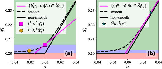
Figure 6: Running Algorithm 1 on the 1D sphere-box system in Figure 3 from the nominal configuration $(\bar{q}_{0}^{\mathrm{o}},\bar{q}_{0}^{\mathrm{a}})=(-0.02,0.2)$. In both subplots, the black solid line represents true non-smooth dynamics, and the black dashed line represents the smoothed dynamics. The yellow circle marks the naive nominal action ${}^{0}\bar{u}=\bar{q}^{\mathrm{a}}_{0}$ and its resulting object configuration ${}^{0}\bar{q}^{\mathrm{o}}_{0}$. Similarly, the magenta square indicates the next nominal action ${}^{1}\bar{u}$ after applying the initial guess heuristics, and the green star shows the final nominal action ${}^{2}\bar{u}$ after running Algorithm 1. The magenta lines depict the set $\{(\hat{q}_{+},\bar{u}+\delta u)|\hat{q}_{+}=\mathbf{B}_{\kappa}\delta u+f_{\kappa}(\bar{q},\bar{u}),\delta u\in\tilde{\mathcal{S}}^{\mathcal{A}}_{\mathbf{\Sigma},\kappa}(\bar{q},\bar{u})\}$ for the different nominal actions. The green, blue, red colored zones denote zones of $q^{\mathrm{o}}_{\text{goal}}$ where the inverse dynamics controller behaves similarly.

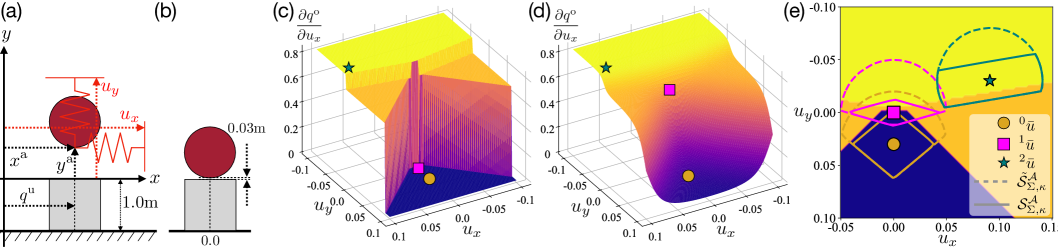
Figure 7: (a) A schematic of the system in Example 5. (b) The nominal configuration $q^{\mathrm{o}}_{0}=0$ and $q^{\mathrm{a}}_{0}=(x^{\mathrm{a}}_{0},y^{\mathrm{a}}_{0})=(0,0.03)$: the ball is hovering above but not touching the box. (c) Gradient landscape of the non-smooth dynamics at the nominal configuration in (b). The blue region at the bottom corresponds to the separation contact mode, the two orange regions the sliding modes, and the yellow region the sticking mode. (d) Gradient landscape of the smoothed dynamics at the same nominal configuration. The dynamics is smoothed with $\kappa=1000$. (e) A-CTR ($\mathcal{S}^{\mathcal{A}}_{\Sigma,\kappa}$) and RA-CTR($\tilde{\mathcal{S}}^{\mathcal{A}}_{\Sigma,\kappa}$) for different $\bar{u}$’s, overlaid on the non-smooth gradient landscape in (c).

Example 4 (1D Pushing).

Revisiting the 1D sphere-box system in Figure 3, we would like to push the box to a goal position $q^{\mathrm{o}}_{\text{goal}}$ by running Algorithm 1. We begin with the nominal configuration $\bar{q}_{0}=(\bar{q}_{0}^{\mathrm{o}},\bar{q}_{0}^{\mathrm{a}})=(-0.02,0.2)$, where the ball nearly touches the box, and a nominal action ${}^{0}\bar{u}=\bar{q}^{\mathrm{a}}_{0}$. The nominal action is depicted by the yellow circle in Figure 6a. Even with the help of dynamics smoothing, the slope at this point is still small and thus provides limited guidance for planning.

Applying the initial guess heuristics in Section 4.2 brings the robot into contact with the object, yielding ${}^{1}\bar{u}=0.0$ (magenta square in Figure 6). The updated ${}^{1}\bar{u}$ produces the new linearized dynamics (magenta line in Figure 6a), whose slope more closely matches the “in contact” piece of the non-smooth contact dynamics. Meanwhile, the dual feasibility constraint (27d) keeps the ball from pulling the box back.

However, the slope at ${}^{1}\bar{u}$ is still quite different from the slope of the in-contact mode. Under this somewhat inaccurate linear approximation of the true dynamics, we further analyze the behavior of the optimizer depending on the given goal configuration $q^{\mathrm{o}}_{\text{goal}}$:

• Green zone: If $q^{\mathrm{o}}_{\text{goal}}$ is in the green zone, the optimizer will move in a positive $u$ direction, correctly moving the box towards the goal. However, as the slope is smaller than the slope of the non-smooth dynamics, the commanded $u$ will overshoot $q^{\mathrm{o}}_{\text{goal}}$.

• Blue zone: If $q^{\mathrm{o}}_{\text{goal}}$ is in the blue zone, then the optimizer will move backwards even though the optimal action is to move forward. This is due to the non-physical behavior caused by smoothing: according to the smoothed linearization, when $u=0$ is commanded, the object will be pushed away by the barrier forces to a location further than $q^{\mathrm{o}}_{\text{goal}}$. To lessen this effect, the optimizer chooses to move backwards.

• Red zone: If $q^{\mathrm{o}}_{\text{goal}}$ is in the red zone, the optimizer would move backwards but stop at the boundary of the red region, which corresponds to the leftmost point in the RA-CTR in Figure 6c. Without dual feasibility (27d), a naive linear model with an ETR will move backwards into the red region to attempt pulling the object.

The analysis above suggests that ${}^{1}\bar{u}$, obtained by applying the initial guess heuristics to ${}^{0}\bar{u}$, is still not ideal for planning: as ${}^{1}\bar{u}$ is located at the boundary between two contact modes which have distinct gradients, a single linear model at ${}^{1}\bar{u}$ approximates neither mode well.

Interestingly, Algorithm 1 can iteratively improve the local linear approximation with the help of dynamics smoothing. Let us consider running Algorithm 1 to reach $q^{\mathrm{o}}_{\text{goal}}=0.22$ from $\bar{q}_{0}$ and ${}^{1}\bar{u}$. At the first iteration, (37) is solved with the RA-CTR in Figure 6a. Due to overshooting caused by underestimating the slope of the true dynamics, ${}^{2}\bar{u}\leftarrow 0.03$. At the second iteration, the optimizer constructs the RA-CTR at ${}^{2}\bar{u}$, which is shown in Figure 6b. As ${}^{2}\bar{u}$ is deeper in penetration, the RA-CTR aligns more closely with $\{u|u\geq 0\}$, the domain of the in-contact piece of the non-smooth dynamics. Moreover, the blue zone under the new RA-CTR, representing the non-physical artifacts caused by smoothing, also shrinks. Under this better local approximation of the non-smooth dynamics, the second iteration returns ${}^{3}\bar{u}=0.0202$, bringing $q^{\mathrm{o}}_{+}$ to within $0.001\mathrm{m}$ of $q^{\mathrm{o}}_{\text{goal}}$.

Example 5 (2D Ball Pushing a Box).

To further illustrate how Algorithm 1 iteratively improves the local linear approximation of the non-smooth contact dynamics, we study a slightly more complex system shown in Figure 7a. The system consists of an unactuated box constrained to slide frictionlessly along the $x$ axis, and an actuated ball that can move in the $xy$ plane and make frictional contact with the box’s top surface.

The non-smooth contact dynamics of this system consists of 4 contact modes: sticking, sliding left, sliding right, and separation. Each mode can be identified with an affine piece in the Piecewise-Affine (PWA) contact dynamics, which is continuous but has discontinuous gradients. Specifically, we examine $\partial q^{\mathrm{o}}_{+}/\partial u_{x}$, the component of $\mathbf{B}_{\kappa}^{\mathrm{o}}=\partial q^{\mathrm{o}}_{+}/\partial u$ that describes how much the object(box) moves along the $x$ axis relative to how much the ball(robot) moves along the same axis. As shown in Figure 7c, $\partial q^{\mathrm{o}}_{+}/\partial u_{x}$ is constant within each mode, but is separated from nearby modes by cliffs. The gradient can be made continuous with dynamics smoothing, which is shown in Figure 7d.

Consider moving the box to $q^{\mathrm{o}}_{\text{goal}}=0.2$ from the initial configuration in Figure 7b: $q^{\mathrm{o}}_{0}=0$ and $q^{\mathrm{a}}_{0}=(x^{\mathrm{a}}_{0},y^{\mathrm{a}}_{0})=(0,0.03)$. Starting with ${}^{0}\bar{u}=q^{\mathrm{a}}_{0}$ (yellow circle in Figure 7) puts the system in the “separation” mode, but accomplishing the task requires the ball to push down and drag the object to the right with friction, which is best done in the “sticking” mode.

We now show that Algorithm 1 is able to iteratively nudge $\bar{u}$ to the “sticking” mode. Similar to Example 4, we first apply the initial guess heuristics, bringing ${}^{0}\bar{u}$ to ${}^{1}\bar{u}=(0,0)$ (magenta square). Looking at the smoothed gradient landscape in Figure 7d, we see that the smoothed $\partial q^{\mathrm{o}}_{+}/\partial u_{x}$ climbs up a lot from $\bar{u}=q^{\mathrm{a}}_{0}$ to $\bar{u}=(0,0)$. Furthermore, after running Algorithm 1 for 2 iterations, the nominal action ${}^{3}\bar{u}$ (green star) reaches the yellow plateau. This sequence of $\bar{u}$’s is plotted in Figure 7d.

Plotting the same $\bar{u}$ sequence over the non-smooth gradient landscape in Figure 7c reveals that $\bar{u}$ jumps from the “separation” mode at the bottom to the “sticking” mode at the top. Without smoothing, mode switches can also be achieved by encoding modes with integer variables and solving the resulting MIP. However, for systems with more contact modes, this approach becomes prohibitively expensive.

Lastly, we plot the A-CTR and the RA-CTR for the above sequence of $\bar{u}$ in Figure 7e. Here we use $\mathbf{\Sigma}=\mathrm{diag}(0.05^{-2},0.05^{-2})$, which bounds $\delta u$ in a circle of radius $0.05$. The curved part of the trust region boundaries arises from the ellipsoidal constraint (25c), whereas the straight part follows from the feasibility constraints (25d) and (25e). Compared with the RA-CTR at ${}^{0}\bar{u}$ (dark yellow), the RA-CTR at ${}^{1}\bar{u}$ (magenta), obtained from applying the initial guess heuristics to ${}^{0}\bar{u}$, approximates the sticking region much better. Furthermore, as ${}^{2}\bar{u}$ (dark green) gets deeper into the “sticking” mode, the straight edge of its RA-CTR aligns more closely with the boundary between sticking and sliding. Finally, compared to the RA-CTRs, the non-relaxed A-CTRs are always smaller. As a result, Algorithm 1 may need more iterations to converge if the RA-CTR constraint in (37d) is replaced by A-CTRs.

4.4 Model Predictive Control

The CTR-based trajectory optimizer in Section 4.1 can be readily turned to a controller through Model Predictive Control (MPC). As shown in Algorithm 2, we obtain the optimal trajectory $u^{\star}_{t}$ by solving (36) with Algorithm 1 (Algorithm 2), only use the first input $u^{\star}_{0}$ to deploy on the true CQDC dynamics Algorithm 2, then re-plan after observing the next configuration. Moreover, we initialize $\mathbf{CtrTrajOpt}$ from the initial guess heuristics (Section 4.2) at the first iteration (Algorithm 2), and from the solution of the previous iteration at later iterations (Algorithm 2).

1 Input: Initial state $q_{0}$, goal state $q_{\text{goal}}$, planning horizon $T$, iterations limit $n_{\mathrm{max}}$, MPC rollout horizon $H$;

2 Output: Lists of visited states $L_{q}$, applied inputs $L_{u}$;

3 $L_{q}\leftarrow[q_{0}]$, $L_{u}\leftarrow[]$;

4 for $t=0$ to $H-1$ do

5    if $t==0$ then

6       $\bar{u}_{0:T-1}\leftarrow$ Apply initial guess heuristics to $q_{t}^{\mathrm{a}}$;

7      

8   else

9       $\bar{u}_{0:T-1}\leftarrow$ Initialize from the previous $u_{0:T-1}^{\star}$;

10      

11   

12   $u_{0:T-1}^{\star}\leftarrow\mathbf{CtrTrajOpt}(q_{t},q_{\text{goal}},\bar{u}_{0:T-1},n_{\mathrm{max}}$);

13    $q_{t+1}=f(q_{t},u_{0}^{\star})$;

14    $L_{q}$.append($q_{t+1}$), $L_{u}$.append($u_{0}^{\star}$);

15   

return$\;L_{q},\;L_{u}$

Algorithm 2 MPC Rollout ($\mathbf{MPC}$)

In Example 6, we demonstrate the effectiveness and scalability of the proposed MPC on the IiwaBimanual example, which has many more contact modes compared to the simple examples we have considered so far.

Example 6 (MPC on IiwaBimanual).

Consider the planar IiwaBimanual system where each iiwa arm has 4 of the 7 available DOFs locked, constraining its motion to the $xy$ plane. The system is tasked with moving a cylindrical object to a desired location. From the initial configuration $q^{\mathrm{o}}_{0}=(q^{\mathrm{o}}_{x},q^{\mathrm{o}}_{y},q^{\mathrm{o}}_{\theta})=(0.65,0,0)$, we command a relative large rotation to reach $q^{\mathrm{o}}_{\text{goal}}=(0.65,0.1,5\pi/6)$. The controller is rolled out in closed-loop for $35$ steps, and the resulting trajectories are displayed in Figure 8.

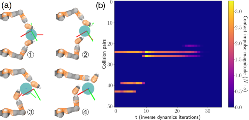
Figure 8: Visualization for Example 6. (a) Visualization of key frames of the closed-loop sequence, with the current $q^{\mathrm{o}}$ and the goal $q^{\mathrm{o}}_{\text{goal}}$ displayed as frames. (b) Visualization of contact forces of every potential collision pair in the IiwaBimanual system.

The contact forces in Figure 8b tells us that the controller is able to scalably search across local changes in contact modes and arrive at a different contact sequence than the initial configuration.

5 Local MPC Experiments

In this section, we investigate evaluate the performance of the CTR-based MPC in Algorithm 2 under the CQDC dynamics constraints. We are particularly interested in answering the following questions:

• How does R-CTR compare with CTR and ETR?

• Does the method successfully reach a diverse set of goals on complex systems such as dexterous hands?

To answer these questions and demonstrate the scalability of our method, we conduct statistical analysis on two contact-rich robotic systems:

• the planar IiwaBimanual system in Example 6, which comprises of 3 unactauted DOFs, 6 actuated DOFs and 29 collision geometries. The whole system is constrained to the $xy$ plane, with gravity pointing along the negative $z$ direction. The bucket measures $0.28\mathrm{m}$ in diameter. The task is to rotate the object, a cylindrical bucket, to target $SE(2)$ poses.

• the 3D AllegroHand system, which comprises 6 unactauted DOFs, 16 actuated DOFs and 39 collision geometries. The object, a $6\mathrm{cm}$ cube, is unconstrained. The hand’s wrist is welded to the world frame. The task is to reorient the cube to target $SE(3)$ poses.

5.1 Experiment Setup

5.1.1 Goal Generation

When evaluating the proposed MPC statistically, the success rate depends on which goals are commanded from which initial configurations. For local optimization, selecting these pairs is nontrivial: goals that are too easy are uninformative, while those requiring highly non-local movements are beyond the scope of local stabilization.

For both the IiwaBimanual and AllegroHand systems, we generate about 1000 pairs of initial conditions and goals which are locally reachable yet far enough to be challenging for MPC. Details about the goal generation scheme can be found in Section A.3.

The sampled pairs are shown in the scatter plots in Figure 9, which exhibit a broad distribution, indicating a high level of diversity in the samples. Moreover, as we only care about moving the object to desired configurations, we do not generate robot goal configurations.

5.1.2 Evaluation Metrics

We evaluate the performance of MPC by comparing the difference between $q^{\mathrm{o}}_{\text{final}}$, the final object configuration reached by the by Algorithm 2, and $q^{\mathrm{o}}_{\text{goal}}$, the goal object configuration. As we are only concerned with reaching object goals, we set the robot-related entries in the cost matrix $\mathbf{Q}$ in (37) to $0$, and rely on the action cost (37b) and the CTR constraint (37d) to stay close to the linerization points.

We split the object configuration ${q^{\mathrm{o}}}$ into a quaternion $Q$ and a position $p$: ${q^{\mathrm{o}}}\coloneqq(Q,p)$, both expressed relative to the world frame. We divide the error in ${q^{\mathrm{o}}}$ into a translation error $\|p_{\text{goal}}-p_{\text{final}}\|$, and an rotation error $\Delta\theta(Q_{\text{goal}},Q_{\text{final}})$, where $\Delta\theta(\cdot,\cdot)$ returns the angular difference between two unit quaternions.

5.1.3 Implementation Details

The numerical experiments are run on a M2 Max Macbook Pro with 64GB of RAM. We use the same open-sourced implementation of the CQDC dyanmics as in Pang et al. (2023). The convex subproblem (37) in Algorithm 1 is solved with Mosek ApS (2024).

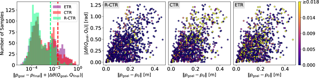
(a) Iiwa Bimanual

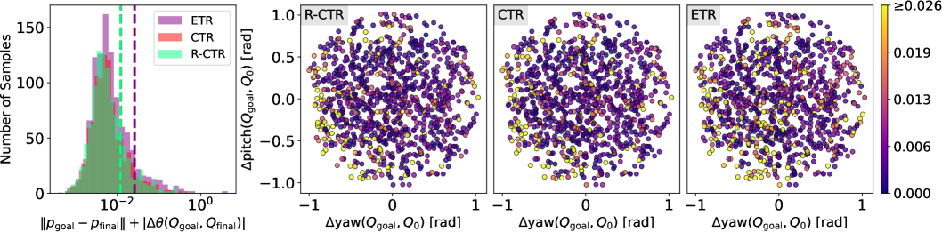
(b) Allegro Hand

Figure 9: Results for running Algorithm 2 with R-CTR, CTR and ETR constraints on the pairs of goals and initial conditions generated in Section 5.1.1. The histogram shows how many samples reached a specified error in the $x$ axis, where error is defined as $\|p_{\text{goal}}-p_{\text{final}}\|+|\Delta\theta(Q_{\text{goal}},Q_{\text{final}})|$. The dotted lines in the histogram represent the average errors. Some dotted lines are barely visible due to overlapping (their values are available in Table 2). Each dot in the scatter plot corresponds to a pair of an initial condition $q^{\mathrm{o}}_{0}$ and a goal $q^{\mathrm{o}}_{\text{goal}}$. Color of the dots is determined by the error: warmer colors indicate bigger errors. The three scatter plots in each row share the same color scale, whose maximum value is the average of the errors for reaching the goals with ETR. (a) For IiwaBimanual, the $x$ axis of the scatter plots is the position difference between $q^{\mathrm{o}}_{0}$ and $q^{\mathrm{o}}_{\text{goal}}$, the $y$ axis the angular difference. (b) For AllegroHand, as the position difference is small for all goals, the $x$ axis shows the yaw angle difference between $q^{\mathrm{o}}_{0}$ and $q^{\mathrm{o}}_{\text{goal}}$, and the $y$ axis the pitch angle difference. The roll, pitch and yaw axes are defined in Figure 14a.

5.2 Effect of Trust Region Radius $\mathbf{\Sigma}$ and Rollout Horizon $H$

In this section, we explore how the two parameters affect the performance of our MPC scheme on both the IiwaBimanual and AllegroHand systems. We also study how these parameters interplay with different trust region formulations, including R-CTR, CTR and ETR. We measure performance in terms of average tracking errors for the goals selected in Section 5.1.1.

As we sweep the two parameters, we fix the planning horizon $T=1$ in Algorithm 2, since increasing $T$ does not improve performance (see Section A.4 for details). Furthermore, we use $n_{\mathrm{max}}=2$ IiwaBimanual and $n_{\mathrm{max}}=3$ for AllegroHand.

5.2.1 Trust Region Radius

How does the trust region radius $\mathbf{\Sigma}$ affect the performance of R-CTR, CTR and ETR? To answer this question, we run Algorithm 2 on both systems with different trust region radii. We set $\mathbf{\Sigma}$ to a constant scaling of the identity matrix, i.e. $\mathbf{\Sigma}=r^{-2}\mathbf{I}$ where $r\in\mathbb{R}_{+}$ is the radius. The results are illustrated in Figure 10a and b, where we measure performance by the average tracking errors for the goals generated in Section 5.1.1.

On both systems, we observe less performance difference between the trust region variants as the radius $r$ shrinks. This is because the feasibility constraints (24d) and (24e) would less likely become active, simply due to the ellipsoid in (24a) being small. However, smaller $r$ also leads to larger tracking errors, as the MPC lacks sufficient authority to progress towards the goal. As $r$ increases, performance initially improves but then starts degrade as $r$ becomes too large, allowing the MPC solution may drift too far from the linearization point.

For IiwaBimanual, we find that R-CTR performs the best among the trust region variants: ETR can be overly relaxed, while CTR can be somewhat restrictive. In contrast, on AllegroHand, all trust region variants behave more similarly, suggesting that AllegroHand may activate the feasibility constraints less frequently than IiwaBimanual. We hypothesize that IiwaBimanual more frequently encounters the unilateral contact scenario in Figure 5a, whereas AllegroHand typically operates in the bilateral contact regime depicted in Figure 4a.

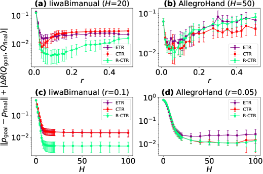
Figure 10: How tracking errors, defined as the sum of translation and rotation errors, change with different trust region radius $r$ ($\mathbf{\Sigma}=r^{-2}\mathbf{I}$) and rollout horizon $H$. The plotted curves denote the average error for the goals generated in Section 5.1.1, and the error bars denote $0.1\sigma$ where $\sigma$ is the standard deviation.

5.2.2 Rollout Horizon $H$

In Figure 10(c) and (d), we examine how performance changes as the MPC rollout horizon $H$ increases. As expected, the tracking errors decrease initially and then plateau for both systems. For IiwaBimanual, R-CTR again outperforms ETR and CTR in terms of average tracking error. On AllegroHand, both CTR-based approaches display comparable performance; although they still outperform ETR, their respective error bars overlap significantly.

For large $H$ ($\geq 80$), while IiwaBimanual’s error curves remain stable, AllegroHand’s curves trend slightly up with larger variances. We attribute this to numerical instability: since AllegroHand has an order of magnitude more collision pairs than IiwaBimanual, numerical issues in collision detection and CQDC dynamics evaluation are more likely to occur. Such issues sometimes destabilize MPC, terminating a run with large final errors.

5.3 Can Our Method Reach Goals?

Finally, for all initial condition and goal pairs generated in Section 5.1.1, we run Algorithm 2 and analyze the results using the metrics in Section 5.1.2. A subset of the MPC hyperparameters is summarized in Table 1.

System	$T$	$n_{\max}$	$r$	$H$
IiwaBimanual	1	2	0.10	20
AllegroHand	1	3	0.05	50

Table 1: MPC hyperparameters: $T$ and $n_{\mathrm{max}}$ are defined in Algorithm 1; $r$ is the trust region radius ($\mathbf{\Sigma}=r^{-2}\mathbf{I}$); $H$ is the MPC rollout horizon in Algorithm 2. These parameters are chosen based on Figure 10.

As shown in Figure 9, MPC with R-CTR achieves the lowest average error on both IiwaBimanual and AllegroHand. As Figure 9 combines rotation and translation errors, we present them separately in Table 2 to better illustrate their relative magnitudes. Notably, MPC with R-CTR also achieves the lowest variance.

	IiwaBimanual		AllegroHand
	Trans. [mm]	Rot. [mrad]	Trans. [mm]	Rot. [mrad]
R-CTR	2.0 (11.5)	2.1 (10.1)	2.2 (5.7)	9.8 (26.9)
CTR	9.4 (30.9)	8.9 (33.3)	2.2 (5.6)	9.9 (28.3)
ETR	8.6 (23.8)	9.6 (37.9)	4.5 (53.8)	21.4 (136.4)

Table 2: Mean translation and rotation errors for the combined errors in Figure 9. Each cell displays the mean (std).

On IiwaBimanual, R-CTR does significantly better than CTR and ETR. In contrast, for AllegroHand, the advantage of R-CTR over the other variants is much more nuanced. This corroborates our analysis in Section 5.2.1.

We also report the wall clock time for the most time-consuming steps in Algorithm 2, shown in Table 3. For AllegroHand, $\mathbf{CtrTrajOpt}$ is considerably slower due to its high-dimensional state and action space, as well as the larger number of collision pairs. The slowness is further compounded by our CQDC dynamics implementation, which has not yet been optimized to leverage problem sparsity. Among the three trust region variants, ETR is the fastest due to the absence of feasibility constraints. In contrast, CTR is the slowest, as it enforces both primal and dual feasibility.

Time unit [ms]		IiwaBimanual	AllegroHand
Per IGH		16.8 (0.05)	32.0 (0.6)
Per $\mathbf{CtrTrajOpt}$	R-CTR	5.1 (0.4)	99.2 (28.6)
	CTR	7.0 (0.2)	205.7 (32.5)
	ETR	2.4 (0.2)	52.9 (21.8)
Per $q_{t+1}=f(q_{t},u_{0}^{\star})$		0.9 (0.05)	5.92 (0.38)

Table 3: Breakdown of the average runtime (wall clock) for Algorithm 2. IGH stands for Initial Guess Heuristic. Each cell displays the mean (standard deviation).

6 Stabilization under Second-Order Dynamics

In Section 5, we presented results for running MPC on the CQDC dynamics (8). However, although the CQDC dynamics removes the force-at-a-distance effect from smoothing, it is still different from real contact physics: not only are second-order effects ignored, it also introduces a small gap between objects undergoing sliding friction (Pang and Tedrake, 2021, Section IV-A2), which is an artifact known as “hydroplaning” (Tedrake, 2023, Appendix B) shared by contact dynamics formulations that utilize Anitescu’s convex relaxation for contact dynamics (Anitescu, 2006).

In this section, we would like to understand how the gap between the CQDC and real physics affect MPC performance in more realistic settings. Specifically, we focus on answering the question: can the MPC controller using the CQDC dynamics perform closed-loop stabilization i) on high-fidelity simulated second-order dynamics, and ii) on hardware?

6.1 Implementation Heuristics for Second-order Dynamics

Fast forwarding to the goal-tracking results in Figure 11, we can see the performance degradation caused by the physics gap is significant. Rather than re-implementing Algorithm 2 with second-order dynamics and a contact model without the hydroplaning artifact, we would like to understand how far we can push CQDC-based MPC through practical adjustments. Specifically, we introduce two modifications to Algorithm 2 which have empirically boosted MPC performance on second-order dynamics (which we denote by the symbol $f_{\text{2nd}}$) . The modified MPC algorithm is summarized in Algorithm 3.

Firstly, instead of running MPC as quickly as possible, we compute a longer trajectory (usually 1-2 seconds) using Algorithm 2 for multiple steps ($H>1$) (Algorithm 3), roll out $L_{u}$ in its entirety on the second-order dynamics (Algorithm 3), and repeat. Although we can re-plan at a higher rate by simply replacing the CQDC dynamics ($f$ in Algorithm 2 of Algorithm 2) with $f_{\text{2nd}}$, we observed that doing high-rate MPC without waiting for the system to stabilize is inconsistent with the quasi-dynamic nature of the CQDC model. In practice, we found CQDC-based MPC works better when we let the system stabilize to an equilibrium before re-planning.

Secondly, we apply the initial guess heuristics more frequently to compensate for the side effects of the hydroplaning artifact. When running trajectories generated by Algorithm 2 open-loop on second-order dynamics, we observed that the robot sometimes loses contact with the object. We hypothesized that this is caused by the hydroplaning artifact of the CQDC dynamics, which allows the robot to exert sliding friction forces on the object without actually touching it. As the hydroplaning artifact does not exist for sticking friction (Anitescu, 2006), we can alleviate hydroplaning by regularly pulling the robot back into contact with object using the initial guess heuristics (Section 4.2). Specifically, in Algorithm 2, instead of only applying the initial guess heuristics at the first iteration (Algorithm 2 to Algorithm 2), we apply it at every iteration to the corresponding $q_{t}^{\mathrm{a}}$.

We denote this modified version of MPC with the symbol $\mathbf{MPC}_{\text{Proj}}$ in Algorithm 3 of Algorithm 3, where the subscript denotes the projection back to the contact manifold, which is the effect of applying the initial guess heuristics.

1 Input: Initial state $q_{0}$, goal state $q_{\text{goal}}$, planning horizon $T$, iterations limit $n_{\mathrm{max}}$, MPC rollout horizon $H$, number of re-plans $N$;

2 $i\leftarrow 0$;

3 while $q_{\mathrm{goal}}$ not reached $\mathrm{and}$ $i<N$ do

4    $q_{0:H}^{\star},u_{0:H-1}^{\star}\leftarrow\mathbf{MPC}_{\text{Proj}}(q_{0},q_{\text{goal}},T,n_{\text{max}},H)$;

5    $q_{\text{final}}\leftarrow$ Apply $u_{0:H-1}^{\star}$ to $f_{\text{2nd}}$;

6    $q_{0}\leftarrow q_{\text{final}}$;

7    $i\leftarrow i+1$

Algorithm 3 MPC with 2nd-order Dynamics $f_{\text{2nd}}$

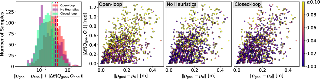
(a) Iiwa Bimanual

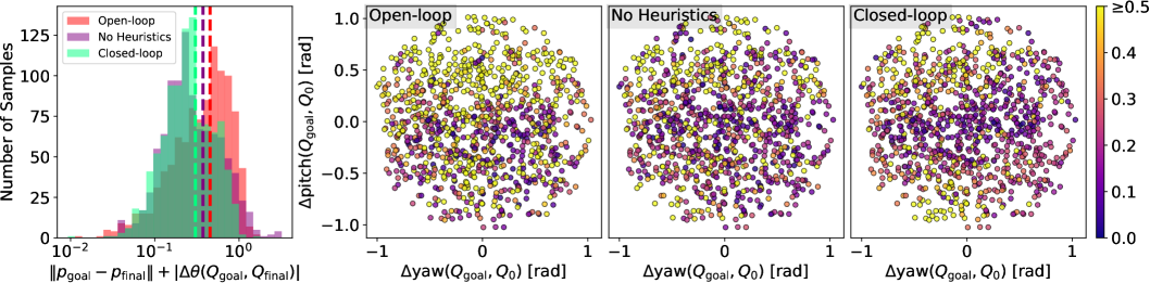
(b) Allegro Hand

Figure 11: Results for running the three variants of Algorithm 3, namely open-loop, no heuristics and close-loop, on the pairs of goals and initial conditions generated in Section 5.1.1. All figure elements follow the same definitions used in Figure 9.

6.2 Experiment Setup

We evaluate Algorithm 3 using the same final-distance-to-goal metric proposed in Section 5.1.2 on both IiwaBimanual and AllegroHand. Hyperparameter choices are summarized in Section A.5. For each system, we run two ablation variants of our algorithm, each omitting a crucial component.

• Closed-loop. This is running Algorithm 3 as is with multiple re-plans ($N>1$).

• No Heuristics. We replace $\mathbf{MPC}_{\text{proj}}$ with the $\mathbf{MPC}$ defined in Algorithm 2. In other words, we apply the initial guess heuristics only at the first iteration in MPC, instead of at every iteration.

• Open-loop. This can be interpreted as reducing feedback rate to the extreme: there is no re-planning at all. Instead, we plan a long trajectory that gets the object all the way to the goal and run it open-loop.

Simulation Setup. We incorporate the IiwaBimanual and AllegroHand systems presented in Section 5 into Drake (Tedrake and the Drake Development Team, 2019), which employs a complete second-order dynamics model along with state-of-the-art contact solvers (Castro et al., 2023) that do not have the hydroplaning effect. We maintain identical collision geometries, robot controller stiffness, and friction coefficients between the CQDC dynamics and Drake.

Hardware Setup. We keep the MPC and physical parameters of the system, such as robot feedback gains, object shape, mass, and friction, consistent between Drake and hardware.

We measure the object pose utilizing the OptiTrack motion capture system. Passive spherical reflectors are sufficient for the bucket in IiwaBimanual. For the cube in AllegroHand, in order to not alter the collision geometry with external markers, we embed light-emitting active markers in the cube. In addition, we post-process the cube pose by solving an inverse kinematics problem that projects the raw OptiTrack measurement out of penetration with the Allegro hand.

6.3 Results & Discussion

We plot the results of our experiments in Figure 11, and display the translation and rotation errors separately in Table 4. We discuss some of our findings from the experiments.

	IiwaBimanual		AllegroHand
	Trans. [m]	Rot. [rad]	Trans. [m]	Rot. [rad]
Open-loop Sim	0.033	0.115	0.011	0.443
	(0.152)	(0.191)	(0.007)	(0.286)
No-Heuristics Sim	0.041	0.066	0.015	0.358
	(0.156)	(0.153)	(0.017)	(0.335)
Closed-loop Sim	0.020	0.039	0.014	0.290
	(0.065)	(0.079)	(0.009)	(0.197)
Open-loop HW	0.016	0.056	0.014	0.323
	(0.019)	(0.064)	(0.007)	(0.256)
Closed-loop HW	0.013	0.024	0.018	0.258
	(0.016)	(0.038)	(0.011)	(0.215)

Table 4: Translation and rotation errors for simulation (Sim) and hardware (HW) experiments. Each cell displays the mean (standard deviation).

6.3.1 Closed-loop vs. Open-loop

Closed-loop MPC clearly outperforms open-loop on both systems. This suggests that feedback is still crucial to reduce object tracking errors despite the gap between CQDC and second-order dynamics.

6.3.2 AllegroHand vs. IiwaBimanual

The average errors from closed-loop MPC is much smaller on IiwaBimanual, which we attribute to the Allegro task’s inherently difficulty. As reaching goal poses on the Allegro often requires lifting the cube (Figure 14b), any slip can cause the cube to slide back to the palm, resetting progress and resulting in large errors. In contrast, on IiwaBimanual, the bucket remains on a tabletop, so slipping merely slows progress without eliminating it.

Challenges due to slipping is also evident in the distribution of tracking errors in the scatter plots in Figure 11b. Under the closed-loop MPC, Allegro’s tracking error remains low for large yaw angles when pitch angle is near zero, because the cube’s bottom face stays close the palm for such goals. In other goal orientations requiring more lift, the cube is less supported by the palm, increasing the risk of losing grip.

6.3.3 Closed-loop vs. No Heuristics

Although the initial guess heuristics only slightly reduces the mean error (see the histograms in Figure 11), it significantly lower the incidence of large errors (i.e., those close to or exceeding 1). Such large errors usually happen when the object falls off the supporting surface (Figure 13d and Figure 14d) after contact is lost during MPC. By regularly applying the initial guess heuristics, the robot is constantly pulled back to the object, greatly reducing the chances of losing contact. As demonstrated in Figure 13b and Figure 14c, although lost contact occurred and caused some error, the object did not fall, thanks to the initial guess heuristics.

Moreover, applying the initial guess heuristics results in cleaner, shorter trajectories. Once contact is lost during the execution of Algorithm 3(e.g. Figure 13), the subsequent $\mathbf{MPC}$ step (Algorithm 3) typically starts by commanding a large robot movement to reestablish contact. However, under the closed-loop variant of Algorithm 3 where the initial guess heuristics is applied more frequently, this movement is significantly smaller.

In fact, for each pair of iniditial and goal configurations, we can compute the path length travelved by the robot as follows:

$$\text{Robot Path Length}\;=\;\int_{0}^{t_{\text{final}}}\|\dot{q}^{\mathrm{a}}(t)\|_{2}\,\mathrm{d}t,$$ (39)

where $t_{\text{final}}$ is the duration of the experiment and ${q}^{\mathrm{a}}(t):\mathbb{R}\rightarrow\mathbb{R}^{n_{\mathrm{a}}}$ the robot trajectory. As shown in Figure 12, closed-loop MPC results in shorter robot path lengths.

6.3.4 Hardware Experiments

Using voxel-grid down-sampling, we get 50 uniformly-spaced pairs of initial states and goals for each system from the pairs used for simulation experiments. Shown in the last two rows of Table 4, the average errors of hardware experiments are comparable to those of simulation. All hardware and simulation videos are available in an interactive plot on our project website.

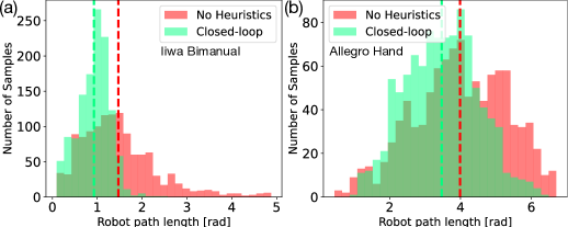
Figure 12: Robot Path Length Comparison between the Closed-loop and No Heuristics variants of Algorithm 3. Dotted vertical lines indicate the mean values of each color-coded sample set.

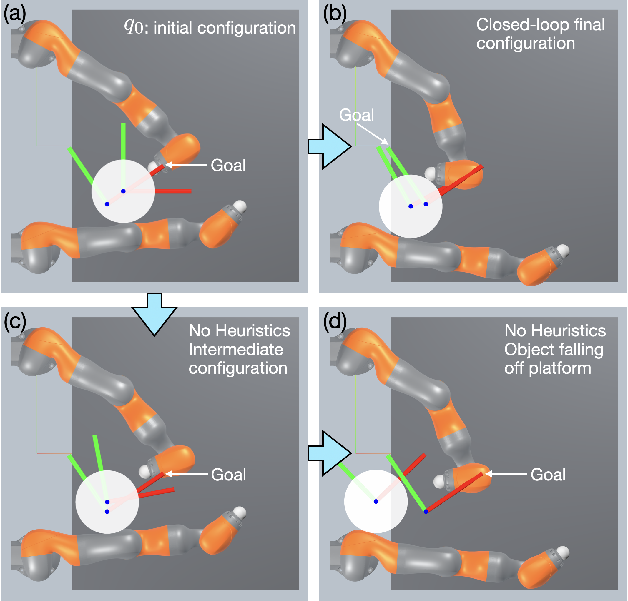
Figure 13: Failures of Algorithm 3 on Iiwabimanual. The dark gray box represents the table top which supports the bucket. The light gray area represents empty space.

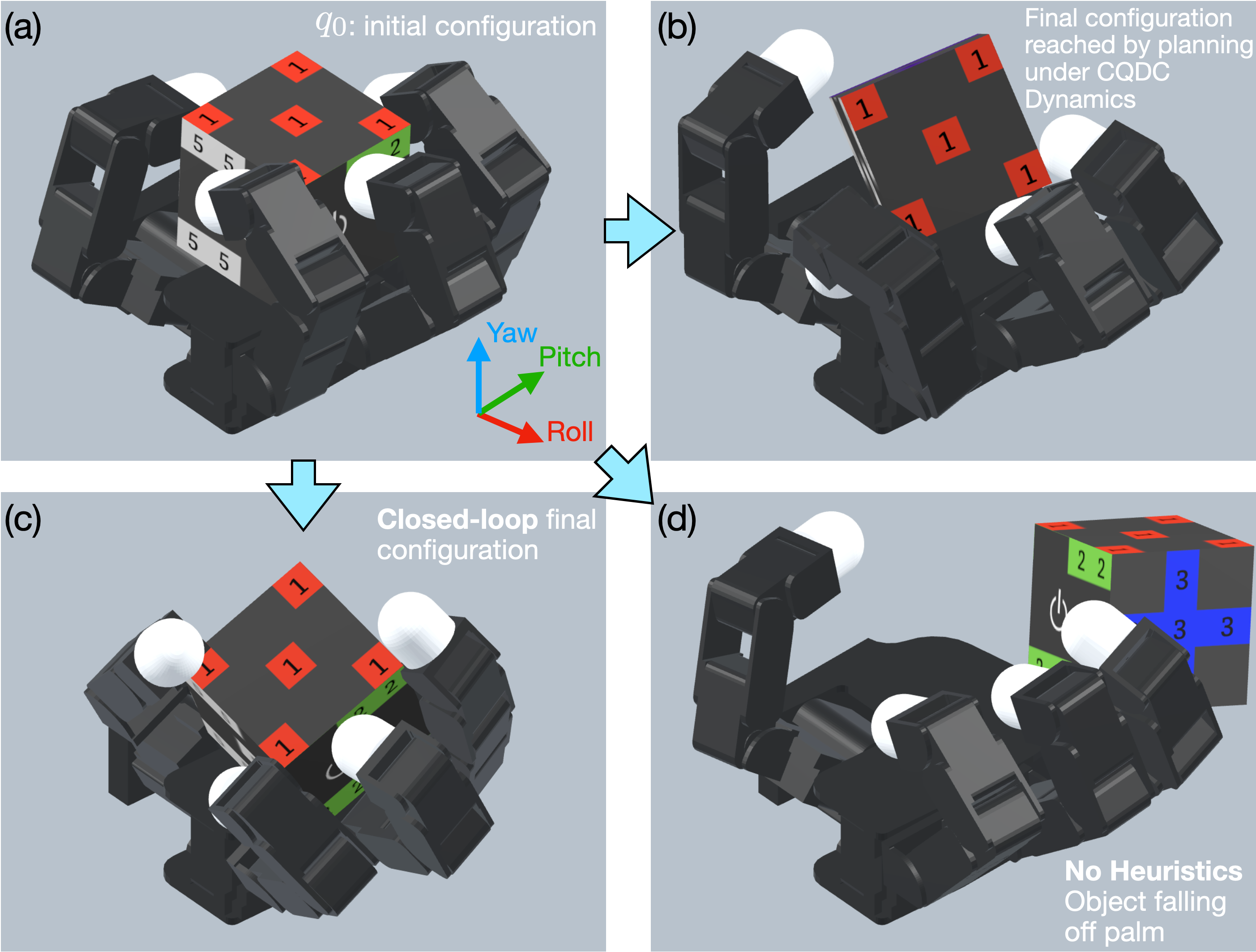
Figure 14: Failures of Algorithm 3 on AllegroHand.

7 Generating Goal-conditioned Contact Configurations

Through our method presented in Section 4, as well as the results in Section 5 and Section 6, we have shown how our proposed MPC allows successful stabilization to local goals.

However, relying solely on finite-horizon MPC formulations can be limiting if the goal is sufficiently “far away”. Specifically, goals that are more difficult to reach require the controller to momentarily make suboptimal actions in order to be optimal in the long run. Such problems inherently cannot be addressed solely by greedy finite-horizon MPC, as illustrated by key examples in Figure 15. To tackle such problems, classical motion planning and RL literature either resort to sophisticated exploration strategies or utilize dynamic programming to estimate a long-horizon value function.

To efficiently conduct long-horizon planning for contact-rich manipulation, we utilize two key insights. The first insight comes from dynamic programming: knowledge of key intermediate states allows us to decompose a difficult long-horizon problem into multiple shorter subproblems in which greedy strategies can be more effective. For the planar-pushing example in Figure 15, consider the configuration in which the ball is at the bottom of the box as opposed to the top. If the planner had i) seen this configuration before and ii) known that this configuration is significantly more advantageous for pushing the box upward using local control, it can attempt to go towards this advantageous configuration first before attempting to establish contact with the box.

Next, we use the fact that because we have full control of the actuated DOFs, it is possible to leverage collision-free motion planning to move from one configuration to another without reasoning about contact dynamics (provided that a feasible path exists). This allows us to abstract away the details of collision-free motion planning at when we plan contact interactions, and assume that the robot can teleport from one configuration when the object is at a stable configuration. For instance, in the planar-pushing example in Figure 15, we can freely search for a good pusher configuration to push the box upwards without having to worry about the details of which path the robot has to take.

In this section, we leverage the CTR and our proposed MPC method to first search for key configurations for reaching given goals. As these configurations are almost always on the contact manifold, we refer to them as contact configurations. In the next section, we will show how we can chain these contact configurations together.

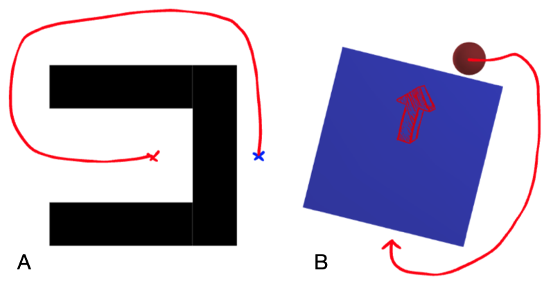
Figure 15: Difficult cases for greedy finite-horizon MPC that require long-horizon exploration capabilities. A. A classical example for path-finding where the robot needs to go from the red X to the blue X. Note that the robot needs go back first, momentarily suffering an increase in Euclidean distance, before it can proceed towards the blue X and reach the goal. B. A similar planar-pushing example in manipulation, where the goal is to push the box upwards. From this configuration, the agent must break contact and travel all around to the back of the box, causing no effect in making progress towards the goal in terms of box movement, in order to push the box up.

7.1 Problem Specification

Given a current configuration of the object ${q^{\mathrm{o}}}$ and some goal configuration $q^{\mathrm{o}}_{g}$, we ask: what is a good robot configuration $q^{\mathrm{a}}$, if we want the resulting full configuration $q=(q^{\mathrm{a}},q^{\mathrm{u}})$ to be advantageous for driving ${q^{\mathrm{o}}}$ to $q^{\mathrm{o}}_{g}$ with local MPC? Formally, we write this optimization problem as

$$\min_{q^{\mathrm{a}}}\;\; C(q^{\mathrm{a}};{q^{\mathrm{o}}},q^{\mathrm{o}}_{g})$$ (40a)

s.t. $$q_{lb}^{\mathrm{a}}\leq q^{\mathrm{a}}\leq q_{ub}^{\mathrm{a}},$$ (40b)

$$\phi_{i}(q^{\mathrm{a}},q^{\mathrm{o}})\geq 0\quad\forall i,$$ (40c)

where (40b) are joint-limit constraints, (40c) enforce non-penetration constraints for every collision pair indexed by $i$, and $\eqref{eq:nonlinear-grasp-sampling:cost}$ is our cost criteria for judging how fit $q^{\mathrm{a}}$ is in driving ${q^{\mathrm{o}}}$ to $q^{\mathrm{o}}_{g}$. Our cost $C$ consists of two terms: the finite-horizon value function of the MPC policy (Section 7.1.1), and a regularization term for robustness (Section 7.1.2).

7.1.1 Finite-Horizon Value Function of the MPC Policy

A natural way to query the fitness of $q^{\mathrm{a}}$ is to utilize the cost of our finite-horizon MPC problem (36a) incurred from the MPC rollout defined in Algorithm 2,

$$V(q^{\mathrm{a}};{q^{\mathrm{o}}}, q^{\mathrm{o}}_{g})=\|q^{\mathrm{o}}_{g}-q^{\mathrm{o}}_{T}\|^{2}_{\mathbf{Q}}+\sum^{T-1}_{t=0}\|u_{t}-u_{t-1}\|^{2}_{\mathbf{R}},$$ (41a)

s.t. $$q_{0:T},u_{0:T-1}=\textbf{MPC}(q_{0},q^{\mathrm{o}}_{g},T,n_{\mathrm{max}},H),$$ (41b)

$$q_{0}=(q^{\mathrm{a}},q^{\mathrm{o}}).$$ (41c)

We note that although MPC rollout in Algorithm 2 accepts a full configuration $q_{g}$ as a goal, we can give it unactuated configurations only ($q^{\mathrm{o}}_{g}$) by setting the cost terms of the actuated objects to zero, $\mathbf{Q}_{a}=\mathbf{0}$, as we did in Section 5.1.2. In addition, due to the efficiency of the MPC controller, the finite-hozion value function can be quickly queried online. However, the landscape of this value function, as visualized for a simple problem in Figure 16, is multi-modal with many local minima and maxima. This hints at the necessity of global optimization when we search for the minimizers of (41).

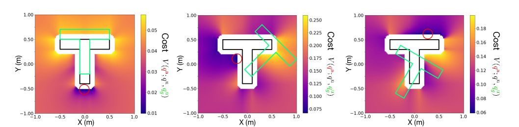
Figure 16: Visualization of the landscape of (41) for the planar pusher-T example inspired by (Chi et al., 2024). The black T corresponds to the current object configuration ${q^{\mathrm{o}}}$, and the green T the goal object configuration $q^{\mathrm{o}}_{g}$. The landscape corresponds to the position of the round pusher $q^{\mathrm{a}}$, colored with the cost function $V({q^{\mathrm{a}}};{q^{\mathrm{o}}},q^{\mathrm{o}}_{g})$. The red pusher configuration corresponds to the global optima of the landscape.

7.1.2 Robustness Regularizer

Is the value function in (41) sufficient as a cost? Although it correctly evaluates the fitness of a given ${q^{\mathrm{a}}}$ in terms of closed-loop goal reaching, we found that there may be cases where multiple configurations are equally fit, yet one configuration provides more robustness compared to others.

For example, consider the task of pushing the ball slightly to the right in Figure 17. Both configurations are nearly equal in the goal-reaching cost (see Table 5); yet, the configuration in Figure 17a would be preferred in practice, as both fingers can be used to reject small disturbances.

To formalize this notion of robustness, we take inspiration from classical grasping metrics (Ferrari and Canny, 1992; Dai et al., 2018; Li et al., 2023), as well as the connection between the RA-CTR and the classical wrench set in Section 3.5. Specifically, we adopt a worst-case metric (Ferrari and Canny, 1992) that reasons about the maximum wrench a grasp can resist along any direction. Geometrically, this quantity corresponds to the maximum-inscribed sphere in the wrench set.

Formally, consider a unit vector $v\in\mathbb{R}^{n_{q_{\mathrm{u}}}}$. Then, the radius of the maximum-inscribed sphere within the wrench set can be described as the following mini-max problem,

$$r({q^{\mathrm{a}}},{q^{\mathrm{o}}})\coloneqq\min_{v} \max_{r\in\mathbb{R}}\;r$$ (42a)

s.t. $$\|v\|=1$$ (42b)

$$rv\in\mathcal{W}_{\mathbf{\Sigma},\kappa}^{\mathcal{A}}(\bar{q}=({q^{\mathrm{a}}},{q^{\mathrm{o}}}),\bar{u}=q^{\mathrm{a}}).$$ (42c)

To evaluate this quantity, we first make a polytopic approximation of the wrench set $\mathcal{W}_{\mathbf{\Sigma},\kappa}^{\mathcal{A}}$ by sampling from the RA-CTR using a rejection sampling scheme. This scheme i) first samples from the ETR ellipsoid and ii) rejects samples that do not obey feasibility constraints (this is the same procedure which generated the samples in Figure 5). Then, we fit a convex hull to these samples using the Qhull library.

Once we have a polytopic representation of the convex set in $H$-rep, (i.e. $\{z|\mathbf{a}_{\mathcal{W},i}^{\top}z+b_{\mathcal{W},i}\leq 0\;\forall i\}$), we can find $r$ by solving a variant of the Chebyshev center problem,

$$\max_{r\geq 0}\; r$$ (43a)

s.t. $$\|a_{i}\|_{2}r+b_{i}\leq 0\quad\forall i.$$ (43b)

7.1.3 Total Cost

We combine the two costs in Section 7.1.1 and Section 7.1.2 use a weighting term $\alpha\in\mathbb{R}_{\geq 0}$:

$$C({q^{\mathrm{a}}};{q^{\mathrm{o}}},q^{\mathrm{o}}_{g})=V({q^{\mathrm{a}}};{q^{\mathrm{o}}},q^{\mathrm{o}}_{g})-\alpha r({q^{\mathrm{a}}};{q^{\mathrm{o}}})^{2},$$ (44)

where we note that the radius is subtracted as it is a reward.

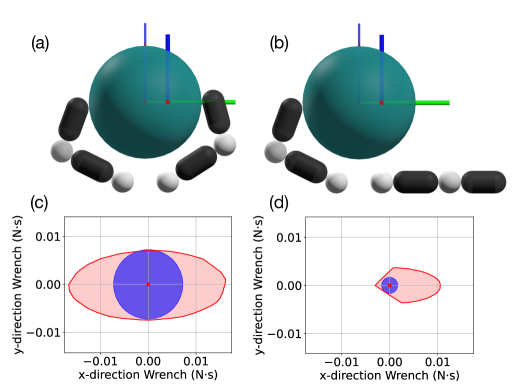
Figure 17: Top Row: Comparison of two configurations (a) and (b) for the 2D planar hand system in Figure 5. Although both configurations are advantageous for moving the object to the goal, they share the same MPC value function cost (Table 5). Bottom Row: Plot of the wrench set (illustrated in red) and the maximum inscribed sphere (blue), where (c) corresponds to configuration (a) and (d) corresponds to (b). Note that configuration (a) has a much larger inscribed sphere due to the anti-podal grasp.

Configuration	(a)	(b)
MPC value function $V$	$2.82\times 10^{-4}$	$2.16\times 10^{-4}$
Max inscribed sphere radius	$7.12\times 10^{-3}$	$1.68\times 10^{-3}$

Table 5: Comparison of MPC value function cost and maximum inscribed sphere radius for two configurations in Figure 17.

7.2 Solving (40) by Sampling-based Optimization

Solving (40) is challenging, as i) the gradient of the cost function is quite difficult to obtain (Li et al., 2023), and ii) it requires global search, as evidenced by the nonconvex cost landscape in Figure 16. As a result, we resort to a simple sampling-based search which samples from the feasible set of (40) by rejection sampling, then chooses the best sample.

However, due to the high variance of this process in high-dimensional spaces, as well as the complexity of navigating high-dimensional configuration spaces, we found that directly applying this strategy is not very effective beyond simple planar problems. To scale the sampling-based search to AllegroHand, we introduce a few heuristic changes to make this optimization more tractable, which we detail in Section A.6.

Figure 18: Initial actuator configurations found by our method for (a) yaw $0^{\circ}$ to $45^{\circ}$, (b) yaw $45^{\circ}$ to $90^{\circ}$, and (c) pitch $0^{\circ}$ to $90^{\circ}$. The initial configuration of the cube is marked with a long and thin triad, while the goal configuration of the cube a short and thick triad.

Task	Position [mm]	Rotation [mrad]	Time [s]
Yaw $0^{\circ}\!\to\!45^{\circ}$	12.05 (3.49)	32.41 (27.14)	57.83 (2.08)
Yaw $45^{\circ}\!\to\!90^{\circ}$	9.85 (10.88)	15.72 (21.08)	57.28 (0.72)
Pitch $0^{\circ}\!\to\!90^{\circ}$	21.42 (8.91)	32.12 (32.03)	57.84 (0.73)

Table 6: Performance of our algorithm for finding initial actuator configurations. Results are obtained with $10$ repeated runs. Each run is optimized using $1000$ samples. Each cell displays the mean (standard deviation).

7.3 Results

We test the performance of our method on the AllegroHand system. We first set up three representative pairs of initial and goal configurations for the cube, then run our algorithm to solve (40), whose solution corresponds to the optimal initial configuration of the Allegro hand. Then, we evaluate the fitness of the solution by rolling out MPC (Algorithm 2) from the found initial configuration, and record the error between the final rollout and the goal configurations.

Results in Table 6 indicate that our method achieves error on the order of $10$mm in position, and $30$ mrad ($1.7^{\circ}$) in orientation. Moreover, the discovered initial hand configurations in Figure 18 agree with our intuition on how the cube should be grasped if we want to move the cube towards the goals.

We note that the given result was obtained with $1000$ samples on the reduced-order model. Reducing the number of samples for lower computation time is possible, but would result in higher variance in performance. In addition, we found that other types of motions, such as pitch $0^{\circ}$ to $-90^{\circ}$, or rotation along the $x$-axis (roll), are physically very difficult on the Allegro hand.

8 Global Planning with Roadmaps

Using the method for generating contact configurations in Section 7, we present a simple recipe for global search, in which we chain local plans together to efficiently reach global goals which are challenging for local MPC. Our method, inspired by the Probabilistic Roadmap (PRM)(Choset et al., 2005), consists of an offline phase in which the roadmap is constructed, and an online phase where we reach arbitrary goals using the roadmap.

8.1 Roadmap Construction

In the offline phase, we build a roadmap in which the vertices are grasping configurations and the edges are local plans that transition between these configurations.

We present the roadmap construction method in Algorithm 4. The set of contact configurations $R$ in Algorithm 4 are generated by solving (40) for $q^{\mathrm{o}}$’s from a set of stable object configurations which sufficiently cover the object workspace. For each pair of configurations $(q_{i},q_{j})$ in $R$, we first try to reach $q^{\mathrm{o}}_{j}$ from $q_{i}$ by running MPC (Algorithm 4), and then reach $q^{\mathrm{a}}_{j}$ by standard collision-free motion planning (Algorithm 4). This procedure is illustrated in Figure 19. We repeat this procedure and add all successful connections to the roadmap.

1 Input: MPC Parameters: $T$, $n_{\mathrm{max}}$ and $H$;

2 Output: Sets of vertices $V$ and edges $E$;

3 $V\leftarrow\emptyset$, $E\leftarrow\emptyset$;

4 Generate contact configurations $R\coloneqq\{(q^{\mathrm{o}}_{i},q^{\mathrm{a}}_{i})\}_{i=1}^{m}$ ;

5 for ordered pair $q_{i}\coloneqq(q^{\mathrm{o}}_{i},q^{\mathrm{a}}_{i}),q_{j}\coloneqq(q^{\mathrm{o}}_{j},q^{\mathrm{a}}_{j})$ in $R$ do

6    $q_{0:H},u_{0:H-1}\leftarrow\mathbf{MPC}(q_{i},q^{\mathrm{o}}_{j},T,n_{\mathrm{max}},H)$;

7    $q_{H:M},u_{H:M-1}\leftarrow\mathbf{CollisionFree}(q_{H},q_{j})$;

8    if $\mathbf{MPC}$ and $\mathbf{CollisionFree}$ both successful then

9       $V$.add($q_{i}$), $V$.add($q_{j}$);

10       $E$.add($q_{i}$, $q_{j}$, $(q_{0:M},u_{0:M-1})$);

11      

12   

return$\;V,\;E$

Algorithm 4 Roadmap Construction

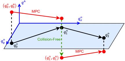
Figure 19: Illustration of roadmap construction described by Algorithm 4. The vertical axis represents the actuator configuration ${q^{\mathrm{a}}}$, while the horizontal plane the space of object configurations ${q^{\mathrm{o}}}$. To connect the vertices $q_{0}:=(q^{\mathrm{o}}_{0},q^{\mathrm{a}}_{0})$ and $q_{1}:=(q^{\mathrm{o}}_{1},q^{\mathrm{a}}_{1})$, we first plan from $q_{0}$ to $q^{\mathrm{o}}_{1}$ with MPC, reaching the top red dot. As the top red dot and $q_{1}$ share the same object configuration $q^{\mathrm{o}}_{1}$, we can connect them with a collision free planner.

We further note that in the special case of manipulating objects with geometric symmetries (such as AllegroHand), a single grasping configuration can represent multiple equivalent configurations. For example, a single grasping configuration for a cube can be expanded into $24$ distinct configurations, due to the cube’s $24$ rotational symmetries. By exploiting this property, the same grasp and action sequence can be used to generate multiple edges in the roadmap.

Consider the cube configuration in Figure 20a, which corresponds to the identity rotation (i.e. no rotation). By leveraging symmetry, we can reach its 24 rotational symmetries using just three basic operations: i) yaw from $0^{\circ}$ to $90^{\circ}$, ii) yaw from $0^{\circ}$ to $-90^{\circ}$ and iii) pitch from $0^{\circ}$ to $90^{\circ}$. These three operations require just five grasps in total: 2 for each yaw and 1 for the pitch (see Figure 18). The grasps take about 5 minutes to generate (Table 6). Moreover, connecting each pair of grasping configurations with MPC and collision-free motion planning takes a few seconds (Table 3), keeping the total roadmap construction time under 10 minutes. Parallelizing these steps can further reduce computation time.

To verify the robustness of the constructed roadmap, we conducted a random walk on the roadmap on hardware, and recorded 150 successful consecutive edge transitions before hardware failure occurred (the hand overheated). Recording of this experiment can be found in the supplementary video.

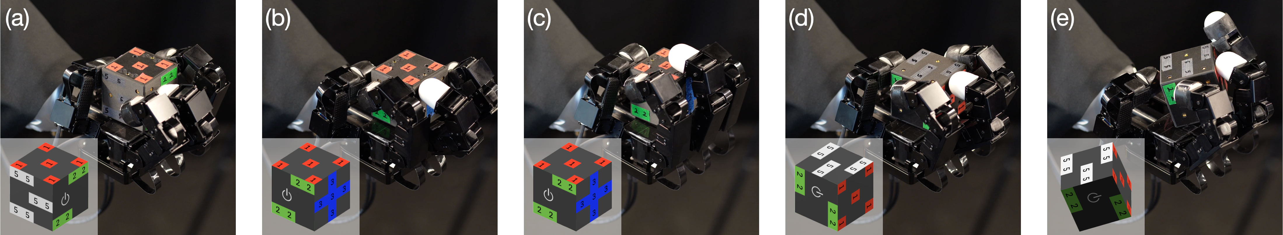
Figure 20: A complete path generated by our roadmap-based global planner. The object configuration in each frame is highlighted at the lower-left corner. (a) shows the starting configuration, which in this example is a vertex already in the roadmap. (b) can be reached from (a) with a $-90^{\circ}$ yaw. (c) has the same object configuration as (b), but the hand has repositioned for a $90^{\circ}$ pitch. (d) is system configuration after the pitch. (e) shows the system reaching the goal configuration from (d). The path (a)-(d) is part of the roadmap and generated offline. (d)-(e) is generated online using collision-free planning and local MPC.

8.2 Inference on a Roadmap

After the roadmap $(V,E)$ is constructed, we can synthesize plans connecting any starting configuration $q_{0}$ to any goal object configuration $q^{\mathrm{o}}_{\text{goal}}$. To do this, we first connect $q_{0}$ and $q^{\mathrm{o}}_{\text{goal}}$ to their respective nearest vertices in the vertex set $V$, which can be done using the same procedure in Algorithm 4 and Algorithm 4 of Algorithm 4. Then, the problem reduces to finding the shortest path between two vertices on a graph, which can be solved with standard methods. An example path generated using this approach is shown in Figure 20. More roadmap planning examples can be found in the supplementary video.

9 Conclusion

Have we solved the problem of planning and control through contact dynamics? Locally—on CQDC dynamics—the proposed MPC with Contact Trust Region constraints can achieve small tracking errors for the vast majority of the goals we sampled based on local reachability criteria. However, we do not understand this problem nearly as well as we do the simple pendulum: not only do we lack solid explanations for the small but non-zero number of planner failures, but we also have yet to fully understand the different roles played by feasibility constraints on IiwaBimanual vs AllegroHand.

Much more remains to be understood for second-order dynamics, both in simulation and on hardware. In particular, keeping the robot in contact with the object, without exploiting the artifact of CQDC dynamics, remains one of the biggest unsolved challenges. Incorporating the CTR constraints in MPC greatly alleviates the problem of lost contact, and the initial guess heuristics empirically helps a bit more. However, we occasionally still observe loss of contact, and its root cause remains unclear.

Nevertheless, the tools presented in this paper already enable capabilities that were previously out of reach for model-based methods. By accounting for the unilateral nature of contact, our contact trust region makes it possible to apply a broad range of robotics algorithms to contact-rich manipulation problems. We hope the MPC, grasp synthesis, and roadmap-based global planning methods introduced here are only a small sample of the many contact-rich manipulation algorithms yet to come. We thank Stephen Proulx, Xinpei Ni, and Velin Dimitrov for building the cube with active OptiTrack markers, and Giovanni Remigi for making the project website.

This work is funded by the Defense Science & Technology Agency Award DST00OECI20300823, Amazon Award PO#2D-15694085, and the Boston Dynamics AI Institute Award Agmd Dtd 8/1/2023.

Appendix A Appendix

A.1 Derivation of (15)

The optimality conditions of (10) consists of the stationarity condition (13) and the relaxed complementary slackness (9), which we reproduce below as

$$\mathbf{P}q_{+}+b-\sum_{i}\mathbf{J}_{i}^{\top}\lambda_{i} =0,$$ (45a)

$$\nu^{\top}_{i}\lambda_{i} =2\kappa^{-1},\quad\forall i.$$ (45b)

The structure of the optimization problem parameters $(\mathbf{P},b,\mathbf{J}_{i},c_{i})$ tells us that $b$ is the only variable dependent on $u$. As the primal and dual variables $q_{+},\lambda_{i}$ are also dependent variables, differentiating both equations w.r.t. $u$ gives us

$$\mathbf{P}\frac{\partial q_{+}}{\partial u}+\frac{\partial b}{\partial u}-\sum_{i}\mathbf{J}_{i}^{\top}\frac{\partial\lambda_{i}}{\partial u} =0$$ (46a)

$$\left(\mathbf{J}_{i}\frac{\partial q_{+}}{\partial u}\right)^{\top}\lambda_{i}+\frac{\partial\lambda_{i}}{\partial u}^{\top}(\mathbf{J}_{i}q_{+}+c_{i}) =0\quad\forall i$$ (46b)

Rewriting in matrix form gives us (15).

We note that the matrix equation (15) is not invertible unless the primal and dual cones defined in (5) were one-dimensional, e.g. $\mathcal{K}=\mathbb{R}_{+}$ and $\mathcal{K^{\star}}=\mathbb{R}_{+}$. This holds in the quadratic programming formulation of contact dynamics (Pang and Tedrake, 2021) where constraints are simple inequalities instead of conic inequalities. For higher-dimensional conic constraints such as (5), differentiating (13) and (12) (instead of (9)) together would produce an invertible systems of equation to which the implicit function theorem can be applied. However, since deriving the derivatives involves complicated matrix differential calculus (Magnus and Neudecker, 2019), we omit its derivation in this paper.

A.2 Proof of Lemma 2

Writing the wrench set gives us

$$\mathcal{W}(\bar{q},\bar{u})=\{w |w=\sum_{i}\mathbf{J}_{\mathrm{o}_{i}}^{\top}\hat{\lambda}_{i}$$ (47a)

$$\hat{\lambda}_{i} =\mathbf{D}_{i}\delta u+\lambda(\bar{q},\bar{u})$$ (47b)

$$\delta u^{\top}\mathbf{\Sigma}\delta u \leq 1$$ (47c)

$$\hat{\lambda}_{i} \in\mathcal{K}^{\star}_{i}\}.$$ (47d)

and we want to prove that the set,

$$\mathcal{M}_{\Sigma,\kappa}^{\mathcal{A},\mathrm{o}}(\bar{q},\bar{u})\coloneqq\{\mathbf{B}^{\mathrm{o}}\delta u+f^{\mathrm{o}}(\bar{q},\bar{u})|\delta u\in\tilde{\mathcal{S}}^{\mathcal{A}}_{\Sigma,\kappa}(\bar{q},\bar{u})\}$$ (48)

is equivalent to

$$\{{q^{\mathrm{o}}_{\texttt{+}}}|\frac{\epsilon}{h}\mathbf{M}_{\mathrm{o}}(\bar{q})(q^{\mathrm{o}}_{+}-\bar{q}^{\mathrm{o}})=h\tau^{\mathrm{o}}+w,w\in\mathcal{W}\}.$$ (49)

To prove this, we utilize Lemma 1 to argue that for any given $\delta u$, the next configuration $\hat{q}_{+}^{\mathrm{o}}$ and contact impulses $\bar{\lambda}_{i}$ that are defined by a linear map on $\delta u$,

$$\hat{q}_{+}^{\mathrm{o}} =\mathbf{B}^{\mathrm{o}}\delta u+f^{\mathrm{o}}(\bar{q},\bar{u}),$$ (50)

$$\hat{\lambda}_{i} =\mathbf{D}_{i}\delta u+\lambda_{i}(\bar{q},\bar{u}),$$ (51)

must jointly satisfy

$$\frac{\varepsilon}{h}\mathbf{M}_{\mathrm{o}}\left(\hat{q}_{+}^{\mathrm{o}}-\bar{q}^{\mathrm{o}}\right)=h\tau^{\mathrm{o}}+\sum_{i}\mathbf{J}_{\mathrm{o}_{i}}^{\top}\hat{\lambda}_{i}.$$ (52)

A.3 Goal Generation for Local MPC

To generate goals that are considered more locally reachable yet far enough to be challenging for the planner, we utilize the following schemes. For the IiwaBimanual environment, we first prescribe some initial state $\bar{q}$ by sampling contact points on the surface of the object and solving inverse kinematics; then, the goals are sampled from the boundary of the action-only object motion set $\mathcal{M}^{\mathcal{A},\mathrm{o}}_{\mathbf{\Sigma},\kappa}(\bar{q},\bar{u})$ with $\bar{u}=\bar{q}^{\mathrm{a}}$. To make the goals sufficiently challenging, we use large ellipsoid radius for the purpose of sampling goals. The resulting goals have maximum $120^{\circ}$ rotation and $0.4m$ translation from the initial state (see Figure 9 for the distrubtion of goals). Similarly, we prescribe some grasp for AllegroHand and sample orientations that have about a $60^{\circ}$ difference from the initial state according to the axis-angle metric. With the above procedure, we sampled $1233$ pairs of initial states and goals for IiwaBimanual and $1000$ pairs for AllegroHand.

We summarize in Table 7 the average amount of translation and rotation between the initial and goal object configurations generated here. These would be the object pose tracking errors if the planning algorithm being evaluated did nothing.

	IiwaBimanual	AllegroHand
Mean $\lVert p_{\text{goal}}-p_{0}\rVert$ [mm]	152	16
Mean $\lvert\Delta\theta(Q_{\text{goal}},Q_{0})\rvert$ [mrad]	356	788

Table 7: Mean translation and rotation differences for pairs of initial and goal object states generated in this section.

A.4 Effect of Planning Horizon for Local MPC

We study how the planning horizon $T$ used in (36) affects the MPC errors. Specifically, for the IiwaBimanual system and the corresponding goals generated using the scheme in Section A.3, we run Algorithm 2 with planning horizon from $1$ to $5$, a maximum iteration of $2$ ($T=1\dots 5$, $n_{\mathrm{max}}=2$ in Algorithm 1), and a MPC rollout horizon $H$ of $10$.

The results are summarized in Table 8. Surprisingly, we found that the planning horizon $T$ has little to no effect on the final error for MPC: our method is able to reach the goals within a tight tolerance for all values of $T$. We believe that this is due to two reasons: i) we have chosen the initial configurations and goals to be reasonably reachable using our trust region, and ii) the CQDC model allows large change in configurations within a single step, so we are able to get away with significantly less horizon compared to other MPC tasks such as dynamic locomotion.

	$T=1$	$T=2$	$T=3$	$T=4$	$T=5$
Translation [mm]	2.02	1.99	1.64	2.11	2.10
	(3.10)	(4.38)	(3.14)	(3.79)	(3.17)
Rotation [mrad]	2.72	3.51	3.25	4.13	5.03
	(0.75)	(1.18)	(2.87)	(1.41)	(2.82)

Table 8: Translation and rotation Errors for IiwaBimanual under different planning horizon $T$. The first row is the mean; the second row (numbers in brackets) is the standard deviation.

A.5 Hyperparameters for 2nd-order Dynamics Stabilization

We use the same $\mathbf{CtrTrajOpt}$ parameters from Table 1. Other important MPC hyperparameters are summarized in Table 9. For closed-loop IiwaBimanual experiments, we use larger $N$ for goals that are further away, while keeping $N\times H$ around $25$. In contrast, as slippage happens a lot more often on the AllegroHand system, we keep $N$ constant for all goals to give MPC more chances to recover.

	$N$ (Number of re-plans)		$H$ (MPC rollout horizon)
System	open-loop	closed-loop	open-loop	closed-loop
IiwaBimanual	1	Variable	25	5
AllegroHand	1	5	50	10

Table 9: Hyperparameters for the MPC in Algorithm 3. No Heurisitcs and Closed-loop share the same parameters.

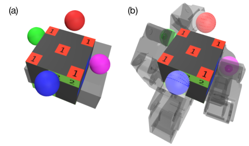
Figure 21: (a) Visualization of the reduced-order system for the Allegro in Section A.6.1, which consists of four spheres. (b) Visualization of the IK result on the optimized solution, mapping the reduced-order system to the full system.

A.6 Heuristics for Generating Allegro Contact Configurations

A.6.1 A Reduced-Order Model

Inspired by (Murray et al., 1994, §5.4), instead of solving (40) directly on the full configuration space of ${q^{\mathrm{a}}}$, we first solve the problem on a reduced-order model, then map the solution to ${q^{\mathrm{a}}}$. For the Allegro hand, our reduced-order model consists of four spheres, each free to move in 3 dimensions with bounding-box joint limits (Figure 21a). Then, we solve for ${q^{\mathrm{a}}}$ by matching the fingertip positions to those of the spheres with Inverse Kinematics (IK), as shown in Figure 21b. Our IK procedure solves the following Quadratic Program (QP) iteratively,

$$\min_{\delta q,p_{+,k}}\;\; \sum_{k}\|p_{+,k}-p_{\text{des},k}\|^{2}$$ (53a)

s.t. $$p_{+,k}=p_{k}+\frac{\partial{p_{k}}}{\partial q}\delta q$$ (53b)

$$\mathbf{J}_{n_{i}}\delta q+\phi_{i}\geq 0$$ (53c)

$$-\varepsilon\mathbf{1}\leq\delta q\leq\varepsilon\mathbf{1},$$ (53d)

where $k$ indexes each fingertip and its corresponding sphere, $p_{\text{des},k}\in\mathbb{R}^{3}$ is the location of the sphere, $p_{k}$ is the location of the fingertips at the current iteration $q$. Note that (53b) corresponds to a linearization of forward kinematics and (53c) enforces non penetration at every iteration. After an optimal $\delta q^{\star}$ is found, we start the next iteration with $q\leftarrow q+\delta q^{\star}$.

A.6.2 Contact Sampling Distribution

Furthermore, we noticed that when we sample from the feasible set of (40), the spheres in the reduced-order model frequently do not fully end up in contact with the cube, resulting in a low robustness metric. Thus, after sampling sphere positions from their respective joint limits, we project the spheres to the nearest point on the surface of the cube, so that we are effectively sampling from a distribution of grasps.

References

- Anitescu (2006) Anitescu M (2006) Optimization-based simulation of nonsmooth rigid multibody dynamics. Mathematical Programming 105(1): 113–143. 10.1007/s10107-005-0590-7. URL https://doi.org/10.1007/s10107-005-0590-7.
- Aydinoglu and Posa (2022) Aydinoglu A and Posa M (2022) Real-time multi-contact model predictive control via admm. In: 2022 International Conference on Robotics and Automation (ICRA). pp. 3414–3421. 10.1109/ICRA46639.2022.9811957.
- Aydinoglu et al. (2022) Aydinoglu A, Sieg P, Preciado VM and Posa M (2022) Stabilization of complementarity systems via contact-aware controllers. IEEE Transactions on Robotics 38(3): 1735–1754. 10.1109/TRO.2021.3120931.
- Boyd and Vandenberghe (2004) Boyd S and Vandenberghe L (2004) Convex optimization. Cambridge university press.
- Castro et al. (2023) Castro A, Han X and Masterjohn J (2023) A theory of irrotational contact fields. arXiv preprint arXiv:2312.03908 .
- Chavan-Dafle et al. (2020) Chavan-Dafle N, Holladay R and Rodriguez A (2020) Planar in-hand manipulation via motion cones. The International Journal of Robotics Research 39(2-3): 163–182. 10.1177/0278364919880257.
- Chen et al. (2022) Chen T, Xu J and Agrawal P (2022) A system for general in-hand object re-orientation. In: Faust A, Hsu D and Neumann G (eds.) Proceedings of the 5th Conference on Robot Learning, Proceedings of Machine Learning Research, volume 164. PMLR, pp. 297–307. URL https://proceedings.mlr.press/v164/chen22a.html.
- Cheng et al. (2022) Cheng X, Huang E, Hou Y and Mason MT (2022) Contact mode guided motion planning for quasidynamic dexterous manipulation in 3d. In: 2022 International Conference on Robotics and Automation (ICRA). pp. 2730–2736. 10.1109/ICRA46639.2022.9811872.
- Cheng et al. (2024) Cheng X, Patil S, Temel Z, Kroemer O and Mason MT (2024) Enhancing dexterity in robotic manipulation via hierarchical contact exploration. IEEE Robotics and Automation Letters 9(1): 390–397. 10.1109/LRA.2023.3333699.
- Chi et al. (2024) Chi C, Xu Z, Feng S, Cousineau E, Du Y, Burchfiel B, Tedrake R and Song S (2024) Diffusion policy: Visuomotor policy learning via action diffusion. The International Journal of Robotics Research .
- Choset et al. (2005) Choset H, Lynch KM, Hutchinson S, Kantor GA and Burgard W (2005) Principles of robot motion: theory, algorithms, and implementations. MIT press.
- Craig (1986) Craig J (1986) Introduction to robotics : mechanics & control. Reading, Mass.: Addison-Wesley Pub. Co. ISBN 0201103265.
- Dai et al. (2018) Dai H, Majumdar A and Tedrake R (2018) Synthesis and Optimization of Force Closure Grasps via Sequential Semidefinite Programming. Cham: Springer International Publishing. ISBN 978-3-319-51532-8, pp. 285–305. 10.1007/978-3-319-51532-8_18. URL https://doi.org/10.1007/978-3-319-51532-8_18.
- Dai et al. (2016) Dai H et al. (2016) Robust multi-contact dynamical motion planning using contact wrench set. PhD Thesis, Massachusetts Institute of Technology.
- Ding et al. (2019) Ding Y, Pandala A and Park HW (2019) Real-time model predictive control for versatile dynamic motions in quadrupedal robots. In: 2019 International Conference on Robotics and Automation (ICRA). pp. 8484–8490. 10.1109/ICRA.2019.8793669.
- Erdmann (1994) Erdmann M (1994) On a representation of friction in configuration space. The International Journal of Robotics Research 13(3): 240–271. 10.1177/027836499401300306. URL https://doi.org/10.1177/027836499401300306.
- Ferrari and Canny (1992) Ferrari C and Canny J (1992) Planning optimal grasps. In: Proceedings 1992 IEEE International Conference on Robotics and Automation. pp. 2290–2295 vol.3. 10.1109/ROBOT.1992.219918.
- Freeman et al. (2021) Freeman CD, Frey E, Raichuk A, Girgin S, Mordatch I and Bachem O (2021) Brax - a differentiable physics engine for large scale rigid body simulation. URL http://github.com/google/brax.
- Graesdal et al. (2024) Graesdal BP, Chia SYC, Marcucci T, Morozov S, Amice A, Parrilo PA and Tedrake R (2024) Towards tight convex relaxations for contact-rich manipulation. arXiv preprint arXiv:2402.10312 .
- Han et al. (2000) Han L, Trinkle J and Li Z (2000) Grasp analysis as linear matrix inequality problems. IEEE Transactions on Robotics and Automation 16(6): 663–674. 10.1109/70.897778.
- Han et al. (2023) Han X, Masterjohn J and Castro A (2023) A convex formulation of frictional contact between rigid and deformable bodies. IEEE Robotics and Automation Letters 8(10): 6219–6226. 10.1109/LRA.2023.3304543.
- Handa et al. (2022) Handa A, Allshire A, Makoviychuk V, Petrenko A, Singh R, Liu J, Makoviichuk D, Van Wyk K, Zhurkevich A, Sundaralingam B, Narang Y, Lafleche JF, Fox D and State G (2022) Dextreme: Transfer of agile in-hand manipulation from simulation to reality. arXiv .
- Howell et al. (2022) Howell T, Gileadi N, Tunyasuvunakool S, Zakka K, Erez T and Tassa Y (2022) Predictive sampling: Real-time behaviour synthesis with mujoco. URL https://arxiv.org/abs/2212.00541.
- Howell et al. (2023a) Howell TA, Cleac’h SL, Brüdigam J, Kolter JZ, Schwager M and Manchester Z (2023a) Dojo: A differentiable physics engine for robotics. URL https://arxiv.org/abs/2203.00806.
- Howell et al. (2023b) Howell TA, Cleac’h SL, Singh S, Florence P, Manchester Z and Sindhwani V (2023b) Trajectory optimization with optimization-based dynamics. URL https://arxiv.org/abs/2109.04928.
- Huang et al. (2020) Huang E, Cheng X and Mason MT (2020) Efficient contact mode enumeration in 3d.
- Jin (2024) Jin W (2024) Complementarity-free multi-contact modeling and optimization for dexterous manipulation. URL https://arxiv.org/abs/2408.07855.
- Kavraki et al. (1996) Kavraki L, Svestka P, Latombe JC and Overmars M (1996) Probabilistic roadmaps for path planning in high-dimensional configuration spaces. IEEE Transactions on Robotics and Automation 12(4): 566–580. 10.1109/70.508439.
- Khandate et al. (2024) Khandate G, Saidi TL, Shang S, Chang ET, Liu Y, Dennis S, Adams J and Ciocarlie M (2024) R times r: Rapid exploration for reinforcement learning via sampling-based reset distributions and imitation pre-training. Autonomous Robots 48(7): 17. 10.1007/s10514-024-10170-8. URL https://doi.org/10.1007/s10514-024-10170-8.
- Kong et al. (2023) Kong NJ, Li C, Council G and Johnson AM (2023) Hybrid ilqr model predictive control for contact implicit stabilization on legged robots. IEEE Transactions on Robotics 39(6): 4712–4727. 10.1109/TRO.2023.3308773.
- Kurtz and Lin (2022) Kurtz V and Lin H (2022) Contact-implicit trajectory optimization with hydroelastic contact and ilqr. URL https://arxiv.org/abs/2202.13986.
- Le Cleac’h et al. (2024) Le Cleac’h S, Howell TA, Yang S, Lee CY, Zhang J, Bishop A, Schwager M and Manchester Z (2024) Fast contact-implicit model predictive control. IEEE Transactions on Robotics 40: 1617–1629. 10.1109/TRO.2024.3351554.
- Le Lidec et al. (2024) Le Lidec Q, Schramm F, Montaut L, Schmid C, Laptev I and Carpentier J (2024) Leveraging randomized smoothing for optimal control of nonsmooth dynamical systems. Nonlinear Analysis: Hybrid Systems 52: 101468. https://doi.org/10.1016/j.nahs.2024.101468. URL https://www.sciencedirect.com/science/article/pii/S1751570X24000050.
- Li et al. (2023) Li AH, Culbertson P, Burdick JW and Ames AD (2023) Frogger: Fast robust grasp generation via the min-weight metric. In: 2023 IEEE/RSJ International Conference on Intelligent Robots and Systems (IROS). pp. 6809–6816. 10.1109/IROS55552.2023.10341806.
- Li et al. (2024) Li AH, Culbertson P, Kurtz V and Ames AD (2024) Drop: Dexterous reorientation via online planning. arXiv preprint arXiv:2409.14562 Available at: https://arxiv.org/abs/2409.14562.
- Li and Todorov (2004) Li W and Todorov E (2004) Iterative linear quadratic regulator design for nonlinear biological movement systems. In: First International Conference on Informatics in Control, Automation and Robotics, volume 2. SciTePress, pp. 222–229.
- Li et al. (2025) Li Y, Han H, Kang S, Ma J and Yang H (2025) On the surprising robustness of sequential convex optimization for contact-implicit motion planning. arXiv preprint arXiv:2502.01055 .
- Lynch and Park (2017) Lynch K and Park F (2017) Modern Robotics: Mechanics, Planning, and Control. Cambridge university press.
- Macklin (2022) Macklin M (2022) Warp: A high-performance python framework for gpu simulation and graphics. https://github.com/nvidia/warp. NVIDIA GPU Technology Conference (GTC).
- Magnus and Neudecker (2019) Magnus JR and Neudecker H (2019) Matrix differential calculus with applications in statistics and econometrics. John Wiley & Sons.
- Marcucci et al. (2017) Marcucci T, Deits R, Gabiccini M, Bicchi A and Tedrake R (2017) Approximate hybrid model predictive control for multi-contact push recovery in complex environments. In: 2017 IEEE-RAS 17th International Conference on Humanoid Robotics (Humanoids). pp. 31–38. 10.1109/HUMANOIDS.2017.8239534.
- Marcucci and Tedrake (2019) Marcucci T and Tedrake R (2019) Mixed-integer formulations for optimal control of piecewise-affine systems. In: Proceedings of the 22nd ACM International Conference on Hybrid Systems: Computation and Control. pp. 230–239.
- Marcucci et al. (2024) Marcucci T, Umenberger J, Parrilo P and Tedrake R (2024) Shortest paths in graphs of convex sets. SIAM Journal on Optimization 34(1): 507–532.
- Mason (1986) Mason MT (1986) Mechanics and planning of manipulator pushing operations. Int. J. Rob. Res. 5(3): 53–71. 10.1177/027836498600500303. URL https://doi.org/10.1177/027836498600500303.
- Mason and Salisbury (1985) Mason MT and Salisbury JK (1985) Robot hands and the mechanics of manipulation. Cambridge, MA, USA: MIT Press. ISBN 0262132052.
- More (1993) More JJ (1993) Generalizations of the trust region problem. Optimization Methods and Software 2(3-4): 189–209. 10.1080/10556789308805542.
- Moré and Sorensen (1983) Moré JJ and Sorensen DC (1983) Computing a trust region step. SIAM Journal on Scientific and Statistical Computing 4(3): 553–572. 10.1137/0904038. URL https://doi.org/10.1137/0904038.
- Mosek ApS (2024) Mosek ApS (2024) MOSEK Optimizer API for Python 10.2.1. URL https://docs.mosek.com/latest/pythonapi/index.html.
- Murray et al. (1994) Murray RM, Sastry SS and Zexiang L (1994) A Mathematical Introduction to Robotic Manipulation. 1st edition. USA: CRC Press, Inc. ISBN 0849379814.
- Niu and Yuan (2010) Niu L and Yuan Y (2010) A new trust-region algorithm for nonlinear constrained optimization. Journal of Computational Mathematics 28(1): 72–86. https://doi.org/10.4208/jcm.2009.09-m2924. URL http://global-sci.org/intro/article_detail/jcm/8508.html.
- Nocedal and Wright (2006) Nocedal J and Wright SJ (2006) Numerical Optimization. Springer.
- Onol et al. (2019) Onol AO, Long P and Padır T (2019) Contact-implicit trajectory optimization based on a variable smooth contact model and successive convexification. In: 2019 International Conference on Robotics and Automation (ICRA). pp. 2447–2453. 10.1109/ICRA.2019.8794250.
- OpenAI et al. (2019) OpenAI, Andrychowicz M, Baker B, Chociej M, Jozefowicz R, McGrew B, Pachocki J, Petron A, Plappert M, Powell G, Ray A, Schneider J, Sidor S, Tobin J, Welinder P, Weng L and Zaremba W (2019) Learning dexterous in-hand manipulation. URL https://arxiv.org/abs/1808.00177.
- Pang et al. (2023) Pang T, Suh HJT, Yang L and Tedrake R (2023) Global planning for contact-rich manipulation via local smoothing of quasi-dynamic contact models. IEEE Transactions on Robotics 39(6): 4691–4711. 10.1109/TRO.2023.3300230.
- Pang and Tedrake (2021) Pang T and Tedrake R (2021) A convex quasistatic time-stepping scheme for rigid multibody systems with contact and friction. In: 2021 IEEE International Conference on Robotics and Automation (ICRA). pp. 6614–6620. 10.1109/ICRA48506.2021.9560941.
- Pang and Tedrake (2022) Pang T and Tedrake R (2022) Easing reliance on collision-free planning with contact-aware control. In: 2022 International Conference on Robotics and Automation (ICRA). IEEE, pp. 8375–8381.
- Posa et al. (2014) Posa M, Cantu C and Tedrake R (2014) A direct method for trajectory optimization of rigid bodies through contact. The International Journal of Robotics Research 33(1): 69–81. 10.1177/0278364913506757.
- Prattichizzo and Trinkle (2008) Prattichizzo D and Trinkle JC (2008) Grasping. Berlin, Heidelberg: Springer Berlin Heidelberg. ISBN 978-3-540-30301-5, pp. 671–700. 10.1007/978-3-540-30301-5_29. URL https://doi.org/10.1007/978-3-540-30301-5_29.
- Shirai et al. (2024a) Shirai Y, Zhao T, Suh HJT, Zhu H, Ni X, Wang J, Simchowitz M and Pang T (2024a) Is linear feedback on smoothed dynamics sufficient for stabilizing contact-rich plans? URL https://arxiv.org/abs/2411.06542.
- Shirai et al. (2024b) Shirai Y, Zhao T, Suh HT, Zhu H, Ni X, Wang J, Simchowitz M and Pang T (2024b) Is linear feedback on smoothed dynamics sufficient for stabilizing contact-rich plans?
- Sorensen (1982) Sorensen DC (1982) Newton’s method with a model trust region modification. SIAM Journal on Numerical Analysis 19(2): 409–426. 10.1137/0719026. URL https://doi.org/10.1137/0719026.
- Stewart and Trinkle (2000) Stewart DE and Trinkle JC (2000) An implicit time-stepping scheme for rigid body dynamics with coulomb friction. Proceedings 2000 ICRA. Millennium Conference. IEEE International Conference on Robotics and Automation. Symposia Proceedings (Cat. No.00CH37065) 1: 162–169 vol.1. URL https://api.semanticscholar.org/CorpusID:10920958.
- Suh et al. (2022a) Suh HJ, Simchowitz M, Zhang K and Tedrake R (2022a) Do differentiable simulators give better policy gradients? In: Chaudhuri K, Jegelka S, Song L, Szepesvari C, Niu G and Sabato S (eds.) Proceedings of the 39th International Conference on Machine Learning, Proceedings of Machine Learning Research, volume 162. PMLR, pp. 20668–20696. URL https://proceedings.mlr.press/v162/suh22b.html.
- Suh et al. (2022b) Suh HJT, Pang T and Tedrake R (2022b) Bundled gradients through contact via randomized smoothing. IEEE Robotics and Automation Letters 7(2): 4000–4007. 10.1109/LRA.2022.3146931.
- Tassa et al. (2012) Tassa Y, Erez T and Todorov E (2012) Synthesis and stabilization of complex behaviors through online trajectory optimization. In: 2012 IEEE/RSJ International Conference on Intelligent Robots and Systems. pp. 4906–4913. 10.1109/IROS.2012.6386025.
- Tedrake (2023) Tedrake R (2023) Underactuated Robotics. URL https://underactuated.csail.mit.edu.
- Tedrake and the Drake Development Team (2019) Tedrake R and the Drake Development Team (2019) Drake: Model-based design and verification for robotics. URL https://drake.mit.edu.
- Todorov (2014) Todorov E (2014) Convex and analytically-invertible dynamics with contacts and constraints: Theory and implementation in mujoco. In: 2014 IEEE International Conference on Robotics and Automation (ICRA). pp. 6054–6061. 10.1109/ICRA.2014.6907751.
- Todorov et al. (2012) Todorov E, Erez T and Tassa Y (2012) Mujoco: A physics engine for model-based control. In: 2012 IEEE/RSJ International Conference on Intelligent Robots and Systems. pp. 5026–5033. 10.1109/IROS.2012.6386109.
- Wensing et al. (2024) Wensing PM, Posa M, Hu Y, Escande A, Mansard N and Prete AD (2024) Optimization-based control for dynamic legged robots. IEEE Transactions on Robotics 40: 43–63. 10.1109/TRO.2023.3324580.
- Werling et al. (2021) Werling K, Omens D, Lee J, Exarchos I and Liu CK (2021) Fast and feature-complete differentiable physics for articulated rigid bodies with contact. arXiv preprint arXiv:2103.16021 .
- Zhang et al. (2023) Zhang S, Jin W and Wang Z (2023) Adaptive barrier smoothing for first-order policy gradient with contact dynamics. In: Krause A, Brunskill E, Cho K, Engelhardt B, Sabato S and Scarlett J (eds.) Proceedings of the 40th International Conference on Machine Learning, Proceedings of Machine Learning Research, volume 202. PMLR, pp. 41219–41243. URL https://proceedings.mlr.press/v202/zhang23s.html.
- Zhong et al. (2022) Zhong YD, Han J and Brikis GO (2022) Differentiable physics simulations with contacts: Do they have correct gradients w.r.t. position, velocity and control? URL https://arxiv.org/abs/2207.05060.