Minimisation of Quasar-Convex Functions Using Random Zeroth-Order Oracles

Abstract

This study explores the performance of a random Gaussian smoothing zeroth-order (ZO) scheme for minimising quasar-convex (QC) and strongly quasar-convex (SQC) functions in both unconstrained and constrained settings. For the unconstrained problem, we establish the ZO algorithm’s convergence to a global minimum along with its complexity when applied to both QC and SQC functions. For the constrained problem, we introduce the new notion of proximal-quasar-convexity and prove analogous results to the unconstrained case. Specifically, we show the complexity bounds and the convergence of the algorithm to a neighbourhood of a global minimum whose size can be controlled under a variance reduction scheme. Theoretical findings are illustrated through investigating the performance of the algorithm applied to a range of problems in machine learning and optimisation. Specifically, we observe scenarios where the ZO method outperforms gradient descent. We provide a possible explanation for this phenomenon.

1 Introduction

In this paper, we study the minimisation problem of the form

$$\min_{x\in\mathcal{X}}\quad f(x)$$ (1)

where $f:\mathbb{R}^{n}\rightarrow\mathbb{R}$ is differentiable, integrable, possibly non-convex and bounded below and $\mathcal{X}\subseteq\mathbb{R}^{n}$ is a non-empty convex set.

To solve Problem 1, several categories of optimisation methods has been proposed in the literature. Most existing methods rely on access to the function’s gradient, limiting their applicability to many real-world scenarios. For instance, in many practical systems, one can only observe the input and output of a Deep Neural Network (DNN) without access to its internal configurations, such as the network structure and weights. Optimisation methods that rely solely on the (noisy) evaluations of the objective function are commonly referred to as zeroth-order (ZO) or derivative-free frameworks (Rios & Sahinidis, 2013; Audet & Hare, 2017). These schemes have attracted increasing interests in recent years due to their success in solving black-box problems arising in machine learning and signal processing, such as automated backpropagation in deep learning (DL) (Liu et al., 2020b) and evaluating the adversarial robustness of DL networks (Goodfellow et al., 2014), where explicit expressions of gradients are expensive to compute (Cartis et al., 2010) or even unattainable (Maass et al., 2021). ZO methods provide a solution to these challenges by estimating gradients using function evaluations.

Multiple ZO algorithms have been developed to solve various optimisation problems, for example, methods inspired by evolutionary strategies (Moriarty et al., 1999), methods based on direct search (Vicente, 2013) (Anagnostidis et al., 2021), and those the rely on unbiased variance-bounded approximators of the gradient (Ghadimi et al., 2016). Recently, (Nesterov & Spokoiny, 2017) proposed and analysed a random ZO oracle based on Gaussian smoothing that yields a gradient estimate of a point by computing the function values of the point and a point in its neighbourhood based on Gaussian sampling. As an unbiased estimator of the gradient of the Gaussian smoothed function, this zeroth-order method is gaining attention in optimisation because of the desirable properties of the Gaussian smoothed function. For example, the Gaussian smoothed function is shown to inherit the convexity and Lipschitzness of the original function and possess Lipschitz gradient as long as the original function is globally Lipschitz (Nesterov & Spokoiny, 2017). Existing results indeed demonstrate its efficacy when applying different optimisation problems. The authors in (Nesterov & Spokoiny, 2017) show that their proposed algorithm, in expectation, converges to an $\epsilon$-optimal point (i.e., $f(x)-f(x^{\ast})\leq\epsilon$) in $\mathcal{O}(n\epsilon^{-1})$ iterations and $\mathcal{O}(n\log(\epsilon^{-1}))$ iterations when applied to a smooth convex function and a smooth strongly convex function, respectively. When applied to a non-smooth convex function, the algorithm converges to an $\epsilon$-optimal point in $\mathcal{O}(n^{2}\epsilon^{-2})$ iterations. They analyse the non-convex smooth case and show the convergence to an $\epsilon$-stationary point (i.e., $\|\nabla f(x)\|\leq\epsilon$) in $\mathcal{O}(n^{2}\epsilon^{-2})$ iterations. Considering non-convex functions, a recent work Farzin & Shames (2024) focuses on solving the minimisation problem with smooth objective functions satisfying Polyak-Łojasiewicz inequality. It is shown that their proposed methods converges to an $\epsilon$-optimal point in $\mathcal{O}(n\epsilon^{-1})$ iterations in the unconstrained case and converges to a neighbourhood of the set of $\epsilon$-optimal points in $\mathcal{O}(\epsilon^{-1})$ iterations in the constrained case where the size of the neighbourhood is proportional to the variance of the norm of the error of gradient estimate constructed by the ZO method. Another work (Pougkakiotis & Kalogerias, 2023) shows that the proximal Gaussian-smoothing ZO oracle converges to an $\epsilon$-stationary point of the smoothed objective function in $\mathcal{O}(\sqrt{n}\epsilon^{-4})$ iterations, when applied to a non-smooth weakly-convex function. In (Vicente, 2013), the author analyses the unconstrained non-convex minimisation, leveraging the direct search method and shows the convergence to an $\epsilon$-stationary point in $\mathcal{O}(n^{2}\epsilon^{-2})$ iterations.

In this paper, we study the application of the Gaussian-smoothing ZO oracle to a class of non-convex functions that satisfy quasar-convexity. Quasar-convexity is a weaker notion than star-convexity and has been found in a number of problems that are closely related to DL. For example, Hardt et al. (2018) shows that the problem of learning linear dynamical systems, which is known to be closely related to recurrent neural networks, satisfies quasar-convexity under some mild assumptions. Wang & Wibisono (2023) shows that generalised linear models with activation functions including leaky ReLU, quadratic, logistic, and ReLU functions, satisfy quasar-convexity. Results from a number of recent research works also suggest that neural networks may satisfy some kind of quasar-convexity Lin et al. (2024); Zhou et al. (2018). Moreover, we are interested in exploring the convergence of the ZO oracle when applied to strong quasar-convex functions. While it is known that Polyak-Łojasiewicz (PŁ) (Polyak, 1964) condition is weaker than strong quasar-convexity (Hinder et al., 2020), it can be seen that a function which is PŁ (or satisfying quadratic growth) and quasar-convex is strongly quasar-convex (Wang & Wibisono, 2023, Lemma 7). Therefore, a number of learning problems, including linear residual networks (in large regions of parameter space) (Hardt & Ma, 2017) and entropy regularised policy gradient optimisation in a class of reinforcement learning problems (Mei et al., 2020), might be of interest.

These applications have spurred exciting algorithmic design and analysis for functions that satisfy quasar-convexity. For example, (Hinder et al., 2020) develops an accelerated first-order algorithm and shows its iteration complexity for both strong quasar-convex and quasar-convex functions. Guminov et al. (2017) studies the convergence of Nemirovski’s conjugate gradients when applied to functions satisfying quasar-convexity and quadratic growth condition. (Nesterov et al., 2018) proposes an accelerated gradient method and shows the convergence when minimising quasar-convex functions. Jin (2020) studies the convergence of stochastic gradient descent when applied to both strong quasar-convex and quasar-convex functions. However, to the best of our knowledge, all the mentioned papers on (strong) quasar-convex function minimisation are leveraging first-order algorithms and our work is the first that studies the convergence of a random zeroth-order method for (strong) quasar-convex functions.

Contributions

In this paper, we study the random ZO oracle in (Nesterov & Spokoiny, 2017) to solve the minimisation problem of a class of quasar-convex functions. First, we consider the unconstrained setting. We show that the random ZO oracle converges to an $\epsilon$-optimal point in $\mathcal{O}(n\epsilon^{-1})$ number of iterations when applied to quasar-convex functions and in $\mathcal{O}(n\log(\epsilon^{-1}))$ iterations when applied to strongly quasar-convex functions. Despite the non-convexity, our results give the same order of iteration complexity as those for convex and strongly convex functions in the literature, respectively. Next, we consider the constrained setting. We introduce a new notion, called proximal quasar-convex, as an analogue to quasar-convexity in non-smooth optimisation. We show that, when the function satisfies proximal quasar-convexity (resp. strongly proximal quasar-convexity), the projected random ZO oracle converges to a neighbourhood of the set of $\epsilon$-optimal points in $\mathcal{O}(n\epsilon^{-1})$ iterations (resp. in $\mathcal{O}(n\log(\epsilon^{-1}))$ iterations). We further note that the size of the neighbourhood can be reduced to values close to zero using the variance reduction scheme.

While the performance of ZO methods have been generally considered inferior to first-order methods, our numerical results show that the random ZO oracle performs better than gradient descent method when learning a linear dynamical system. Indeed, we find that the random ZO oracle can reduce the chance of exploding gradients, which may be a critical issue commonly found in linear dynamical system identification and recurrent neural network training Pascanu et al. (2013). Our finding may shed light on future algorithmic development in recurrent neural network training problem. Lastly, extensive numerical results demonstrate the efficacy of the random ZO oracle in a range of problems arising in machine learning and optimisation.

Outline

In Section 2, we outline the problems of interest and the Gaussian-smoothing ZO oracle. Section 3 presents the main results on convergence results and the iteration complexities of the Gaussian-smoothing ZO oracle when applied to (strongly) quasar-convex function in unconstrained setting and when applied to (strongly) proximal quasar-convex function in constrained setting. In section 4, we discuss the intuition behind the superior performance of ZO method over gradient descent when learning linear dynamical systems. Section 5 offers illustrative examples. Lastly, we conclude our paper and discuss potential future research directions in Section 6. Auxiliary lemmas, proofs of the main theorems, and some complementary materials and additional numerical experiments can be found in the appendix.

Notation:

In this paper, $\mathbb{R}^{n}$, $n\in\mathbb{N}$, denotes the $n$-dimensional Euclidean space with $\langle\cdot,\cdot\rangle$ as the inner product. Let $\|\cdot\|$ be the Euclidean norm of its argument if it is a vector and the corresponding induced operator norm if the argument is a matrix. The projection operator to a closed convex set $\mathcal{X}\subset\mathbb{R}^{d}$, is defined as $\mathrm{Proj}_{\mathcal{X}}(z)\overset{\text{def}}{=}\arg\underset{x\in\mathcal{X}}{\min}\|x-z\|^{2}.$ The expectation operator with respect to a random variable $u$ is denoted by $E_{u}[\cdot].$ For $k\in\mathbb{N}$, we denote by $\mathcal{U}_{k}=(u_{1},\dots,u_{k})$ a set comprising of independent and identically distributed random vectors $\{u_{k}\}_{k>0}$. The conditional expectation over $\mathcal{U}_{k}$ is denoted by $E_{\mathcal{U}_{k}}[\cdot].$ The diameter of a set $\mathcal{X}$ is denoted by $d$ and is equal to $\sup\{\|x_{1}-x_{2}\|:x_{1},x_{2}\in\mathcal{X}\}.$

2 Problems of Interest And Framework

In this paper, we study the performance of a random Gaussian smoothing ZO method for optimising (strong) quasar-convex functions for both unconstrained and constrained cases. The Gaussian smoothed version of $f,$ given by $f_{\mu}:\mathbb{R}^{n}\to\mathbb{R},$ is defined as:

$$f_{\mu}(x)\overset{\mathrm{def}}{=}\frac{1}{\kappa}\int_{\mathbb{R}^{n}}f(x+\mu u)\mathrm{e}^{-\frac{1}{2}||u||^{2}}\mathrm{d}u$$ (2)

$$\;\kappa\overset{\mathrm{def}}{=}\int_{\mathbb{R}^{n}}\mathrm{e}^{-\frac{1}{2}||u||^{2}}\mathrm{d}u=\frac{(2\pi)^{n/2}}{[\det B]^{\frac{1}{2}}}$$

where $u\in\mathbb{R}^{n}$ is sampled from zero mean Gaussian distribution with a positive definite correlation operator $B^{-1}$ and $\mu>0$ is the smoothing parameter. The random oracle $g_{\mu}:\mathbb{R}^{n}\rightarrow\mathbb{R}^{n}$ is defined as (Nesterov & Spokoiny, 2017, Section 3)

$$g_{\mu}(x)\overset{\mathrm{def}}{=}\frac{f(x+\mu u)-f(x)}{\mu}Bu,$$ (3)

where $u\in\mathbb{R}^{n}$ and $B\in\mathbb{R}^{n\times n}$ are defined above. It is shown that $g_{\mu}$ is an unbiased estimator of $\nabla f_{\mu}$; i.e., $\nabla f_{\mu}(x)=E_{u}[g_{\mu}(x)]$. We use this random ZO oracle to update our estimate. To ensure the feasibility of the generated points in the constrained case, we leverage a projection step. In our setting, without any loss of generality, the matrix $B$ is set to the identity matrix. The algorithm is summarised in Algorithm 1, where $x_{0}$ is the initial guess, $\mu>0$ is the smoothing parameter, $h_{k}$ is the step size and $N$ is the number of iterations.

Algorithm 1 Random Min ($\mathrm{RM}_{\mu}$)

1:Input: $x_{0}\in\mathcal{X},\ N\in\mathbb{N},\ \{h_{k}\}_{k=1}^{N},\ \mu>0$

2:for $k=0$ to $N$ do

3:  Sample $u_{k}$ from $\mathcal{N}(0,\mathbb{I})$

4:  Calculate $g_{\mu}(x_{k})$ using $u=u_{k}$ and (3)

5:  Compute $x_{k+1}=\text{Proj}_{\mathcal{X}}\left(x_{k}-h_{k}g_{\mu_{x}}(x_{k})\right)$

6:end for

7:return $x_{N}$

We aim to investigate the performance of Algorithm 1 when applied to quasar-convex functions. First, we consider the unconstrained setting of Problem 1; i.e., $\mathcal{X}=\mathbb{R}^{n}$. Then, we analyse the performance in the constrained setting of Problem 1; i.e., $\mathcal{X}\subset\mathbb{R}^{n}$. Before proceeding further, we need to define quasar-convexity.

Definition 1 (Quasar-convex function).

Let $f:\mathbb{R}^{n}\rightarrow\mathbb{R}$ be a continuously differentiable function, $\gamma\in(0,1],$ $\beta>0$, and $x^{\ast}$ be a minimiser of $f.$ We say that $f$ is $\gamma$-quasar-convex with respect to $x^{\ast}$ if for all $x\in\mathbb{R}^{n}$,

$$f(x^{\ast})\geq f(x)+\frac{1}{\gamma}\langle\nabla f(x),x^{\ast}-x\rangle$$ (4)

and $f$ is $\beta$-strongly-$\gamma$-quasar-convex with respect to $x^{\ast}$ if for all $x\in\mathbb{R}^{n}$,

$$f(x^{\ast})\geq f(x)+\frac{1}{\gamma}\langle\nabla f(x),x^{\ast}-x\rangle+\frac{\beta}{2}\|x^{\ast}-x\|^{2}$$ (5)

Quasar-convexity is found in a number of optimisation problems that are closely related to DL or machine learning Hardt et al. (2018); Wang & Wibisono (2023); Hardt & Ma (2017); Mei et al. (2020). It also possesses benign properties for the ease of analysis. For example, it can be seen that any stationary point of a quasar-convex function is its global minimum and the minimiser of a strongly-quasar-convex function is unique.

Next, we consider the constrained setting of Problem 1. Suppose that $\mathcal{X}\subset\mathbb{R}^{n}$ is a non-empty compact convex set with diameter $d$. Since quasar-convexity is well-defined only for unconstrained problems with the objective being differentiable Hinder et al. (2020), we reformulate the constrained problem to a non-differentiable unconstrained problem and introduce the notion of proximal quasar-convex

Definition 2 (Proximal $\gamma$-quasar-convex Functions).

Let $\gamma\in(0,1]$ and $\beta>0$. Consider $\mathcal{X}\subseteq\mathbb{R}^{n}$ and the function $F(x)=f(x)+l(x)$ where $f:\mathbb{R}^{n}\rightarrow\mathbb{R}$ is differentiable and $l:\mathbb{R}^{n}\rightarrow\mathbb{R}\cup\{\infty\}$ is convex and possibly non-differentiable. Let $x^{\ast}\in\mathcal{X}$ be the minimiser of $F$. We say that $F$ is proximal $\gamma$-quasar-convex with respect to $x^{\ast}$ if for all $x\in\mathcal{X}$,

$$F(x^{\ast})-F(x)\geq\frac{1}{\gamma}\langle Q_{l}(x,a),x^{\ast}-x\rangle,$$ (6)

and $F$ is proximal $\beta$-strongly-$\gamma$-quasar-convex with respect to $x^{\ast}$ if for all $x\in\mathcal{X}$,

$$F(x^{\ast})-F(x)\geq\frac{1}{\gamma}\langle Q_{l}(x,a),x^{\ast}-x\rangle+\frac{\beta}{2}\|x-x^{\ast}\|^{2}.$$ (7)

Here,

$$\begin{split}Q_{l}(x,a)\overset{\mathrm{def}}{=}-\frac{1}{a}(\mathrm{Prox}_{l}(x-a\nabla f(x))-x)\end{split}$$ (8)

with $a$ being a positive scalar and $\mathrm{Prox}_{l}(x)=\arg\underset{z}{\min}(\|z-x\|^{2}+l(z)-l(x))$.

As can be seen in Remark 1, when $l\equiv 0$, the proximal quasar-convexity reduces to quasar-convexity. Indeed, it shares similar properties as quasar-convexity. For example, any fixed point of a proximal quasar-convex function (i.e., $x=\mathrm{Prox}_{l}(x-a\nabla f(x))$) is a global minimum and the minimiser of a proximal strongly-quasar-convex function is unique. Moreover, every proximal strongly-quasar-convex function satisfies proximal error bound condition; see Appendix E. An example of a proximal quasar-convex function is $f(x,y)=x^{2}y^{2}$ over $\mathcal{X}=\{(x,y):x\geq 1\}$ or $\mathcal{X}=\{(x,y):y\geq 1\}$, where $f$ is quasar-convex without constraints and satisfies proximal quasar-convexity with the aforementioned constraints. Also, one can consider $f(x,y)=xy.$ This is not a quasar-convex function, but it is a proximal quasar-convex function over the constraint set $\mathcal{X}=\{(x,y):x\geq 0,y\geq 0\}$

Having this set up, we can consider Problem 1 as

$$\min_{x}\{F(x):=f(x)+\mathcal{I}_{\mathcal{X}}(x)\},$$ (9)

where $\mathcal{I}_{\mathcal{X}}:\mathbb{R}^{n}\to\mathbb{R}\cup\{\infty\}$ is the indicator function of the set $\mathcal{X}$; i.e.,

$$\mathcal{I}_{\mathcal{X}}(x)=\begin{cases}0&x\in\mathcal{X}\\ \infty&x\not\in\mathcal{X}.\end{cases}$$

Therefore, for a constrained problem, Definition 2 is equivalent to

$$f(x^{\ast})-f(x)\geq\frac{1}{\gamma}\langle P_{\mathcal{X}}(x,a),x^{\ast}-x\rangle+\frac{\beta}{2}\|x-x^{\ast}\|^{2},$$

for any $x\in\mathcal{X}$, where

$$P_{\mathcal{X}}(x,a)\overset{\text{def}}{=}\frac{1}{a}[x-\mathrm{Proj}_{\mathcal{X}}(x-a\nabla f(x))].$$ (10)

When $F$ is proximal quasar-convex $\beta=0$ and $\beta>0$ when $F$ is proximal strongly quasar-convex.

3 Main Results

In this section, we present results on the convergence and iteration complexity of Algorithm 1 when applied to quasar-convex functions. The proofs of lemmas and theorems can be found in Appendix A and Appendix B, respectively. In the following, we make a standard Lipschitz gradient assumption on the function $f$.

Assumption 1 (Lipschitz Gradients).

Let $f:\mathbb{R}^{n}\rightarrow\mathbb{R}$ be a continuously differentiable function. Then the gradient of $f$ is said to be globally Lipschitz if there exists a Lipschitz constant $L_{1}>0$ such that

$$\|\nabla f(x)-\nabla f(y)\|\leq L_{1}\|x-y\|,\forall x,y\in\mathbb{R}^{n}.$$ (11)

3.1 Unconstrained Problem

In this subsection, we explore problem 1 with $\mathcal{X}=\mathbb{R}^{n}$. The following lemma characterises the behaviour of $f_{\mu}$ defined in (2), when $f$ is a quasar-convex function.

Lemma 1.

Let function $f:\mathbb{R}^{n}\rightarrow\mathbb{R}$ satisfy Assumption 1 and be a $\gamma$-quasar-convex function with respect to some minimiser $x^{\ast}\in\mathbb{R}^{n}$, then $f_{\mu}$ satisfies the below inequality,

$$\gamma(f_{\mu}(x^{\ast})-f_{\mu}(x))+\mu^{2}L_{1}n\geq\langle\nabla f_{\mu}(x),x^{\ast}-x\rangle$$

The proof of Lemma 1 can be found in Appendix A.

Now, Using Lemma 1, the following theorem and corollary characterise the convergence of Algorithm 1 when the objective function is quasar-convex.

Theorem 1.

Let $f:\mathbb{R}^{n}\to\mathbb{R}$ be $\gamma$-quasar-convex with respect to some minimiser $x^{\ast}\in\mathbb{R}^{n}$ and satisfies Assumption 1. Consider the sequence $\{x_{k}\}_{k\geq 0}$ be generated by Algorithm 1 with step size $h_{k}=h=\frac{\gamma}{4(n+4)L_{1}}$. Let $\mathcal{U}_{k-1}=\{u_{0},u_{1},\dots,u_{k-1}\}.$. Then, for any $N\geq 0$:

$$\frac{1}{N+1}\sum_{k=0}^{N}E_{\mathcal{U}_{k-1}}[f(x_{k})]-f(x^{\ast})\leq\frac{4(n+4)L_{1}}{\gamma^{2}}\frac{\|x_{0}-x^{\ast}\|^{2}}{N+1}+\frac{2\mu^{2}L_{1}n(1+\gamma)}{\gamma}+\frac{\mu^{2}(n+6)^{3}L_{1}}{8(n+4)}.$$ (12)

The proof of Theorem 1 can be found in Appendix B. From the upper bound in Theorem 1, the first right-hand side term of (12) is due to initialisation error and becomes arbitrarily small for $N\rightarrow\infty$. The second and third terms are due to the error caused by the difference between the true function and the smoothed function and using the random oracle defined in (3) instead of gradient of the function. They can become arbitrarily small if $\mu\rightarrow 0$. The next corollary gives a guideline on how to choose the number of iterations and the smoothing parameter $\mu$ for a given specific tolerance $\epsilon$.

Corollary 1.

Adopt the hypothesis of Theorem 1. For a given tolerance $\epsilon>0$, let $R=\|x_{0}-x^{\ast}\|$. If $\mu\leq\sqrt{\epsilon(\frac{4L_{1}n(1+\gamma)}{\gamma}+\frac{(n+6)^{3}}{4(n+4)}L_{1})^{-1}}$ and $\begin{aligned} N\geq\Bigg{\lceil}\frac{4(n+4)L_{1}R^{2}}{\gamma^{2}\epsilon}-1\Bigg{\rceil},\end{aligned}$ then,

$$E_{\mathcal{U}_{N-1}}(f(\hat{x}_{N}))-f(x^{\ast})\leq\dfrac{1}{N+1}\sum_{k=0}^{N}E_{\mathcal{U}_{k-1}}[f(x_{k})]-f(x^{\ast})\leq\epsilon,$$

where $\hat{x}_{N}\overset{\mathrm{def}}{=}\arg\min_{x}[f(x):x\in\{x_{0},\cdots,x_{N}\}].$

The following lemma characterises the behaviour of $f_{\mu}$ defined in (2), when $f$ is a strongly quasar convex function.

Lemma 2.

Let function $f:\mathbb{R}^{n}\rightarrow\mathbb{R}$ satisfy Assumption 1 and be a $\beta$-strongly-$\gamma$-quasar-convex function with respect to some minimiser $x^{\ast}\in\mathbb{R}^{n}$. Then $f_{\mu}$ satisfies the below inequality,

$$\gamma(f_{\mu}(x^{\ast})- f_{\mu}(x))+\mu^{2}L_{1}n-\frac{\beta\gamma}{2}\|x-x^{\ast}\|^{2}\geq\langle\nabla f_{\mu}(x),x^{\ast}-x\rangle$$

The proof of Lemma 2 can be find in Appendix A.

Now, Using Lemma 2, we characterise the convergence of Algorithm 1 when the objective function is strongly quasar-convex.

Theorem 2.

Let $f:\mathbb{R}^{n}\to\mathbb{R}$ be $\beta$-strongly-$\gamma$-quasar-convex with respect to some minimiser $x^{\ast}\in\mathbb{R}^{n}$ and satisfy Assumption 1. Consider the sequence $\{x_{k}\}_{k\geq 0}$ generated by Algorithm 1 with step size $h_{k}=h\leq\min\{\frac{\gamma}{2(n+4)L_{1}},\frac{1}{\gamma\beta}\}$. Then, for any $N\geq 0$, we have

$$\sum_{k=0}^{N}(1-\gamma\beta h)^{N-k}(E_{\mathcal{U}_{k-1}}[f(x_{k})]-f(x^{\ast})) \leq\frac{(1-\gamma\beta h)^{N+1}R^{2}}{2h(\gamma-2(n+4)L_{1}h)}+\frac{\mu^{2}L_{1}n(1+\gamma)}{h\gamma\beta(\gamma-2(n+4)L_{1}h)}$$

$$\qquad+\frac{\mu^{2}L_{1}^{2}(n+6)^{3}}{4\gamma\beta(\gamma-2(n+4)L_{1}h)},$$ (13)

where $\mathcal{U}_{k-1}=\{u_{0},u_{1},\dots,u_{k-1}\},$ $R=\|x_{0}-x^{\ast}\|$.

The proof of Theorem 2 can be found in Appendix B. Given the upper bound provided by Theorem 2, the first right-hand side term of (2) is due to initialisation error and becomes arbitrarily small for $N\rightarrow\infty$. The second and third terms are due to the error caused by the difference between the true function and the smoothed function and using the random oracle defined in (3) instead of gradient of the function.. They can become arbitrarily small if $\mu\rightarrow 0$. The next corollary gives a guideline on how to choose the number of iterations and the smoothing parameter $\mu$ for a given specific tolerance $\epsilon$.

Corollary 2.

Adopt the hypothesis of Theorem 2. For a given tolerance $\epsilon>0,$ let $a=\frac{L_{1}n(1+\gamma)}{h\gamma\beta(\gamma-2(n+4)L_{1}h)},$ $b=\frac{L_{1}^{2}(n+6)^{3}}{4\gamma\beta(\gamma-2(n+4)L_{1}h)},$ and $q=2h(\gamma-2(n+4)L_{1}h).$ If $\mu\leq\sqrt{\frac{\epsilon}{2}(a+b)^{-1}}$ and $\begin{aligned} N\geq\Bigg{\lceil}\frac{1}{\gamma\beta h}\log\left(\frac{R^{2}}{q\epsilon}\right)-1\Bigg{\rceil},\end{aligned}$ then,

$$E_{\mathcal{U}_{N-1}}[f(x_{N})]-f(x^{\ast})\leq\epsilon.$$

Theorems 1 and 2 show that, when $f$ is quasar-convex (resp. strongly quasar-convex), Algorithm 1 achieves the same iteration complexity $\mathcal{O}(n\epsilon^{-1})$ (resp. $\mathcal{O}(n\log(\epsilon^{-1}))$) as for convex functions (resp. strongly convex function) to converge to an $\epsilon$-optimal (i.e., $f(x)-f(x^{\ast})\leq\epsilon$ ) point.

Corollary 3.

Adopting the hypothesis of Theorem 2, for a given tolerance $\epsilon>0,$ let $a=\frac{8L_{1}^{2}n(1+\gamma)}{h\gamma^{3}\beta^{3}(\gamma-2(n+4)L_{1}h)},$ $b=\frac{2L_{1}^{3}(n+6)^{3}}{\gamma^{3}\beta^{3}(\gamma-2(n+4)L_{1}h)},$ and $q=2h\gamma^{2}\beta^{2}(\gamma-2(n+4)L_{1}h).$ If $\mu\leq\sqrt{\frac{\epsilon}{2}(a+b)^{-1}}$ and $\begin{aligned} N\geq\Bigg{\lceil}\frac{1}{\gamma\beta h}\log\left(\frac{8L_{1}R^{2}}{q\epsilon}\right)-1\Bigg{\rceil},\end{aligned}$ then, $E_{\mathcal{U}_{N-1}}[\|x_{N}-x^{\ast}\|^{2}]\leq\epsilon.$

3.2 Constrained Problem

In this subsection, we consider the constrained optimisation problem, where $\mathcal{X}\subset\mathbb{R}^{n}$ is a compact convex set. In the following, we make an assumption on the variance of the random ZO oracle.

Assumption 2.

The variance of oracle $g_{\mu}$ defined in (3) is upper bounded by $\sigma^{2}\geq 0$; i.e.,

$$E_{u}[||g_{\mu}(x)-\nabla f_{\mu}(x)||^{2}]\leq\sigma^{2}.$$

This is a common assumption in the literature of ZO stochastic optimisation; see, for example, Maass et al. (2021); Liu et al. (2020a); Farzin et al. (2025). The variance upper bound $\sigma^{2}$ can be approximated via $E_{u}[\|g_{\mu}(x)\|^{2}]$; see more details in Remark 2 in Appendix A.

Now, we can characterise the convergence and iteration complexity of Algorithm 1 when the function is proximal quasar-convex.

Theorem 3.

Let $F:\mathbb{R}^{n}\to\mathbb{R}\cup\{\infty\}$ be the function defined in (9) and $\mathcal{X}$ be the constraint set defined in (1). Suppose that $F$ is proximal $\gamma$-quasar-convex with respect to $\mathcal{X}$ and some minimiser $x^{\ast}\in\mathcal{X}$ and $f:\mathbb{R}^{n}\to\mathbb{R}$ satisfies Assumption 1. Assume that the constraint set $\mathcal{X}$ is a compact convex set with $d$ as its diameter. Consider the sequence $\{x_{k}\}_{k\geq 0}$ be generated by Algorithm 1 with step size $h_{k}=h=\frac{\gamma}{4(n+4)L_{1}}$. Then, under Assumption 2, for any $N\geq 0$, we have

$$\frac{1}{N+1}\sum_{k=0}^{N}E_{\mathcal{U}_{k-1}}[F(x_{k})]-F(x^{\ast})\leq\frac{4(n+4)L_{1}}{\gamma^{2}}\frac{||x_{0}-x^{\ast}||^{2}}{N+1}+\frac{d\mu L_{1}(n+3)^{3/2}}{\gamma}+\frac{\mu^{2}(n+6)^{3}}{8(n+4)}L_{1}+\frac{2d\sigma}{\gamma},$$ (14)

where $\mathcal{U}_{k-1}=\{u_{0},u_{1},\dots,u_{k-1}\}.$

The proof of Theorem 3 can be found in Appendix B. Given the upper bound provided by Theorem 3, the first right-hand side term of (14) becomes arbitrarily small for $N\rightarrow\infty$. The second and third terms, in turns, can become arbitrarily small if $\mu\rightarrow 0$. The forth term can be made arbitrarily small using the variance reduction technique (See Appendix C for more details). Comparing the bounds in Theorems 3 and 1, besides the terms caused by using the random oracle $g_{\mu}$ instead of the gradient and initialisation error, in the constrained case there exists an extra term, caused by the variance of the random oracle. The next corollary gives a guideline on how to choose the number of iterations and the smoothing parameter $\mu$ for a given specific tolerance $\epsilon$.

Corollary 4.

Adopt the hypothesis of Theorem 3. For a given tolerance $\epsilon>0$, let $R=\|x_{0}-x^{\ast}\|$, $a=\frac{(n+6)^{3}}{8(n+4)}L_{1}$, and $b=\frac{dL_{1}(n+3)^{3/2}}{\gamma}$. If $\mu\leq\frac{\sqrt{b^{2}+4a\epsilon}-b}{2a}$ and $\begin{aligned} N\geq\Bigg{\lceil}\frac{8(n+4)L_{1}R^{2}}{\gamma^{2}\epsilon}-1\Bigg{\rceil},\end{aligned}$ then,

$$E_{\mathcal{U}_{N-1}}(f(\hat{x}_{N})-f(x^{\ast}))\leq\dfrac{1}{N+1}\sum_{k=0}^{N}E_{\mathcal{U}_{k-1}}[f(x_{k})]-f(x^{\ast})\leq\epsilon+\frac{2d\sigma}{\gamma},$$

where $\hat{x}_{N}\overset{\mathrm{def}}{=}\arg\min_{x}[f(x):x\in\{x_{0},\cdots,x_{N}\}].$ Thus, we can guarantee there exists an integer $\tilde{N}$ such for all $N\geq\tilde{N},$ $E_{\mathcal{U}_{N-1}}[f(x_{k})]$ is in a neighbourhood of $f(x^{\ast}).$

As it can be seen, the projected Gaussian smoothing ZO estimate is only guaranteed to converge to a neighbourhood of $\epsilon$-optimal points. In fact, similar phenomenon is observed for other ZO algorithms when solving constrained non-convex problems; see e.g. Ghadimi et al. (2016); Liu et al. (2018). However, the size of the neighbourhood can be made arbitrarily small using a variance reduction scheme (See Remark 4). We leave the details to Appendix C.

Next, we present the convergence of Algorithm 1 when the $f$ is proximal strongly-quasar-convex.

Theorem 4.

Let $F:\mathbb{R}^{n}\to\mathbb{R}\cup\{\infty\}$ be the function defined in (9) and $\mathcal{X}$ be the constraint set defined in (1). Suppose that $F$ is proximal $\gamma$-quasar-convex with respect to $\mathcal{X}$ and some minimiser $x^{\ast}\in\mathcal{X}$ and $f:\mathbb{R}^{n}\to\mathbb{R}$ satisfies Assumption 1. Assume that the constraint set $\mathcal{X}$ is a compact convex set with $d$ as its diameter. Consider the sequence $\{x_{k}\}_{k\geq 0}$ be generated by Algorithm 1 with step size $h_{k}=h\leq\min\{\frac{\gamma}{2(n+4)L_{1}},\frac{1}{\gamma\beta}\}$. Then, under Assumption 2, for any $N\geq 0$, we have

$$\sum_{k=0}^{N}(1-\gamma\beta h)^{N-k}(E_{\mathcal{U}_{k-1}}[F(x_{k})]-F(x^{\ast})) \leq\frac{(1-\gamma\beta h)^{N+1}||x_{0}-x^{\ast}||^{2}}{2h(\gamma-2(n+4)L_{1}h)}+\frac{d\sigma}{h\gamma\beta(\gamma-2(n+4)L_{1}h)}$$

$$\quad+\frac{\mu^{2}L_{1}^{2}(n+6)^{3}}{4\gamma\beta(\gamma-2(n+4)L_{1}h)}+\frac{d\mu L_{1}(n+3)^{3/2}}{2\gamma\beta h(\gamma-2(n+4)L_{1}h)},$$ (15)

where $\mathcal{U}_{k-1}=\{u_{0},u_{1},\dots,u_{k-1}\}.$

The proof of Theorem 4 can be found in Appendix B. Given the upper bound provided by Theorem 4, the first right-hand side term of (4) becomes arbitrarily small for $N\rightarrow\infty$. The third and fourth terms, in turns, can become arbitrarily small if $\mu\rightarrow 0$. The second term can be made arbitrarily small using the variance reduction technique (See Remark 5). We leave the details to Appendix C. Comparing the bounds in Theorems 4 and 2, besides the terms caused by using the random oracle $g_{\mu}$ instead of the gradient and initialisation error, in the constrained case there exists an extra term, caused by the variance of the random oracle. The next corollary gives a guideline on how to choose the number of iterations and the smoothing parameter $\mu$ for a given specific tolerance $\epsilon$.

Corollary 5.

Adopt the hypothesis of Theorem 4. For a given tolerance $\epsilon>0$, let $R=\|x_{0}-x^{\ast}\|$, $a=\frac{L_{1}^{2}(n+6)^{3}}{4\gamma\beta(\gamma-2(n+4)L_{1}h)},$ $b=\frac{dL_{1}(n+3)^{3/2}}{2\gamma\beta h(\gamma-2(n+4)L_{1}h)},$ and $q=2h(\gamma-2(n+4)L_{1}h).$ If $\mu\leq\frac{-b+\sqrt{b^{2}+4a\epsilon}}{2a}$ and $\begin{aligned} N\geq\Bigg{\lceil}\frac{1}{\gamma\beta h_{k}}\log\left(\frac{R^{2}}{q\epsilon}\right)-1\Bigg{\rceil},\end{aligned}$ then,

$$E_{\mathcal{U}_{N-1}}[f(x_{N})]-f(x^{\ast})\leq\epsilon+\zeta(\sigma)$$

where $\zeta(\sigma)=\frac{d\sigma}{h\gamma\beta(\gamma-2(n+4)L_{1}h)}$.

Similarly, the convergence is only guaranteed to a neighbourhood of the functions $\epsilon$-optimal points. However, the size of the neighbourhood can be made arbitrarily small via a variance reduction scheme, as described in Appendix C.

4 ZO Methods Average Landscape in the Neighbourhood

While the performance of ZO methods have been generally considered inferior to first-order methods with less information available, our experiments have shown that it actually performs better than stochastic gradient method when learning a linear dynamical system. In this section, we will examine this phenomenon, which may shed light on future algorithmic development on learning linear dynamical systems and recurrent neural network training.

Let $f\colon\mathbb{R}^{n}\to\mathbb{R}$ be a twice differentiable function. Recall that each update is given by $x_{k+1}=x_{k}-h_{k}g_{\mu}(x_{k})$ for some step size $h_{k}>0$ and some gradient approximation $g_{\mu}(x_{k})$ with $\mathbb{E}[g_{\mu}(x_{k})]=\nabla f_{\mu}(x_{k})$. Therefore, given the iterate $x_{k}$ at the $k$-th iteration, the expected is

$$\mathbb{E}[x_{k+1}|x_{k}]=x_{k}-h_{k}\nabla f(x_{k})-h_{k}(\nabla f_{\mu}(x_{k})-\nabla f(x_{k})).$$ (16)

A natural question then arises: Where does the vector $-h_{k}(\nabla f_{\mu}(x_{k})-\nabla f(x_{k}))$ drift the iterate to and how does smoothing take place in the iterate?

To answer this, let us compute the vector explicitly. Nesterov & Spokoiny (2017) shows that the gradient of the Gaussian smoothed function can be written as

$$\nabla f_{\mu}(x)=\frac{1}{\kappa}\int_{\mathbb{R}^{n}}\frac{f(x+\mu u)-f(x)}{\mu}Bue^{-\frac{1}{2}\|u\|^{2}}udu$$

with $\kappa$ defined in (2). Therefore, using Taylor series, we have (4). we can see that

$$\,\nabla f_{\mu}(x)-\nabla f(x)=\frac{1}{\kappa}\int_{\mathbb{R}^{n}}\left(\frac{f(x+\mu u)-f(x)}{\mu}-\langle\nabla f(x),u\rangle\right)Bue^{-\frac{1}{2}\|u\|^{2}}udu$$

$$=\frac{1}{\kappa}\int_{\mathbb{R}^{n}}\left(\frac{f(x)+\mu\nabla f(x)^{T}u+\frac{\mu^{2}}{2}u^{T}\nabla^{2}f(\xi(x,u))u-f(x)}{\mu}-\langle\nabla f(x),u\rangle\right)Bue^{-\frac{1}{2}\|u\|^{2}}udu$$

$$=\frac{\mu}{2\kappa}\int_{\mathbb{R}^{n}}u^{T}\nabla^{2}f(\xi(x,u))uBue^{-\frac{1}{2}\|u\|^{2}}udu$$ (17)

where $\xi(x,u)\in\mathbb{R}^{n}$ is some vector on the line segment between $x$ and $x+u$; i.e., $\xi(x,u)=tx+(1-t)(x+u)$ for some $t\in[0,1]$. Since each $\xi(x,u)$ depends on the direction $u$, it is very hard to compute the integral out. Having said that, the integral sheds light on the information possessed by the vector $\nabla f_{\mu}(x)-\nabla f(x)$.

For simplicity, let us assume the entries of the random vector in Gaussian smoothing to be independently and identically distributed; i.e., $B=I_{n}$. Consider some $u\in\mathbb{R}^{n}$ and write $\xi=\xi(x,u)$ for a shorthand. Suppose that the second derivative is continuous and thus the Hessian $\nabla^{2}f(\xi)$ can be diagonalised as $\nabla^{2}f(\xi)=\sum_{i=1}^{n}\lambda_{i}v_{i}v_{i}^{T}$ for some eigenvectors $\{v_{i}\}_{i=1}^{n}$ and eigenvalues $\{\lambda_{i}\}_{i=1}^{n}$. Moreover, write the vector $u=\sum_{i=1}^{n}a_{i}v_{i}$ as the linear combination of the vectors on the new basis. Putting aside the probability density, then, each vector $u$ carries a weight of $u^{T}\nabla^{2}f(\xi(x,u))u=\sum_{i=1}^{n}\lambda_{i}a_{i}^{2}.$ This implies that the integral $\frac{1}{\kappa}\int_{\mathbb{R}^{n}}u^{T}\nabla^{2}f(\xi(x,u))uBue^{-\frac{1}{2}\|u\|^{2}}udu$ takes the average of the landscape of the neighbourhood of $x$, in the sense that more weight is given to the direction whose curvature is large. Contrary to the issues of exploding or vanishing gradients of gradient descent when learning a linear dynamical system, this “stablises” the gradient approximation and therefore reduces the chance of exploding gradients; see Section 5.1 for numerical results. As a side remark, such inference also applies to other zeroth-order methods, such as uniform smoothing Huang et al. (2022) and coordinate-wise smoothing Chen et al. (2024).

The above development sheds light on the algorithmic design in a recurrent neural network training problem. Having a similar representation as a linear dynamical system identification problem (except for the non-linear transition of the state), it is known that gradient-based learning algorithms encounter the problem of exploding and vanishing gradients; see, e.g., Bengio et al. (1994); Pascanu et al. (2013); Hardt et al. (2018). As Pascanu et al. (2013) hypothesised that the problem of exploding gradient of recurrent neural network occurs when the curvature along some direction explodes, we see that the expected update of Gaussian smoothing ZO oracle (16) avoids the issue by escaping from such direction.

5 Numerical Examples

In this section, we illustrate the performance of Algorithm 1 via extensive numerical examples. In our experiments, we use the performance of gradient descent (GD) as benchmark. Although GD acquires the first-order information of the function and thus is generally considered superior than ZO method, we see that in some of our examples, ZO method performs as good as, or even better than GD. Due to limited space, we have included a subset of scenarios in this section. More scenarios and examples as well as more extensive commentary on the simulations presented below can be found in Appendix F.

5.1 Learning Linear Dynamical System

In this subsection, we evaluate the scheme on the problem of linear dynamical systems identification (LDSI), which is shown to possess quasar-convexity under some assumption in Hardt et al. (2018). Suppose that observations ${(x_{t},y_{t})}_{i=1}^{T}\in\mathbb{R}\times\mathbb{R}$ are generated by a linear time-invariance system $h_{t+1}=Ah_{t}+Bx_{t};\;y_{t}=Ch_{t}+Dx_{t}+\xi_{t},$ where $h_{t}\in\mathbb{R}^{n}$ is the hidden state at time $t$ and accordingly $A\in\mathbb{R}^{n\times n},$ $B\in\mathbb{R}^{n\times 1},$ $C\in\mathbb{R}^{1\times n},$ $D\in\mathbb{R}.$ The parameters of the system ($A,B,C,D$) are unknown and we seek to learn them by minimising $\frac{1}{T}\sum_{i=1}^{T}(y_{t}-\hat{y}_{t})^{2},$ over ($\hat{A},\hat{B},\hat{C},\hat{D}$), where $\hat{h}_{t+1}=\hat{A}\hat{h}_{t}+\hat{B}x_{t};\;\hat{y}_{t}=\hat{C}\hat{h}_{t}+\hat{D}x_{t},$ and $\hat{h}_{0}=0.$ More details can be found in Appendix F.3. In Figure 1 it can be observed the average of the objective function value and its standard deviation over 5 runs in both number of iterations and CPU time. As discussed in Section 4, the ZO method exhibits favourable properties compared to the gradient descent method.

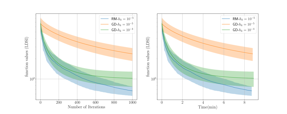
Figure 1: Average of the LDSI objective function value

5.2 Support Vector Machine with smoothed hinge loss function

In this subsection, we illustrate the algorithm’s performance over a real-world task. We train a support vector machine (SVM) on the Breast Cancer dataset Dua & Graff (2019) using Algorithm 1. The SVM loss function we use is the smoothed version of the hinge loss function Hinder et al. (2020) $f(x)=\sum_{i=1}^{m}\phi_{\alpha}(1-b_{i}a_{i}^{T}x),$ where $a_{i}\in\mathbb{R}^{n},$ $b_{i}=\pm 1$ are given by the training dataset ($m=569$ and $n=30$). Function $\phi_{\alpha}(t)=0$ for $t\leq 0$, $\frac{t^{2}}{2}$ for $t\in[0,1]$, and $\frac{t^{\alpha}-a}{\alpha}+\frac{1}{2}$ for $t\geq 1$. When $\alpha=1$ it is convex and for all $\alpha\in[0,1]$, it is smooth and $\alpha$-quasar-convex. We choose $\alpha=0.5,$ $N=10000,$ $\mu=10^{-7},$ and five initial points which are sampled from $\mathcal{N}(0,I_{n})$. We consider seven different step sizes $[10^{-4},5\times 10^{-5},10^{-5},5\times 10^{-6},10^{-6},5\times 10^{-7},10^{-7}].$ To compare the performance of Algorithm 1 and GD, we run each algorithm using each step size and initial value. For each step size and initial point, RM is run for four times and the average is considered. For each step size, the average CPU time (wall-clock time) and decay rate ($1-\frac{f(x_{N})}{f(x_{0})}$) over different initial points are reported in Table 1. The average of the loss function value and its standard deviation, for $h=10^{-4}$, in both number of iterations and CPU time, are presented Figure 6. It can be seen that with the same hyper-parameters, the performance of Algorithm 1 is very similar to GD while having less information available.

Step size	RM		GD
	Time (s)	Decay Rate	Time (s)	Decay Rate
$1\times 10^{-4}$	$8.805$	$97.170$	$8,676$	$97.163$
$5\times 10^{-5}$	$8.925$	$96.693$	$8.708$	$96.714$
$1\times 10^{-5}$	$9.106$	$93.855$	$8.966$	$93.810$
$5\times 10^{-6}$	$9.112$	$91.841$	$9.210$	$91.839$
$1\times 10^{-6}$	$9.374$	$53.010$	$9.738$	$83.934$
$5\times 10^{-7}$	$9.540$	$65.256$	$10.190$	$74.523$
$1\times 10^{-7}$	$9.994$	$45.368$	$11.481$	$45.106$

Table 1: Mean execution time and decay rate for RM and GD algorithms for different learning rates. For all scenarios the two algorithms return almost identical solutions.

6 Conclusions And Future Research Directions

The performance of the Gaussian smoothing ZO random oracles on minimising (strong) quasar-convex functions, with or without constraints, was explored. For the unconstrained problem, the convergence and complexity bounds of the ZO scheme were studied when applied to both strong quasar-convex and quasar-convex loss functions. For the constrained problem, we introduced the notion of proximal quasar-convexity and established the convergence and complexity bounds of the ZO method. We also discussed the phenomenon that the ZO method outperforms stochastic gradient descent when learning a linear dynamical system. A number of numerical examples were presented to illustrate the findings. A future research direction includes the exploration of the constrained case with unbounded constraint set. Another possible future direction is to study minimax problems by taking advantage of the quasar-convexity/concavity structure.

Appendix A Auxiliary Lemmas and more background material

Lemma 3–7 are adopted from (Nesterov & Spokoiny, 2017). The results are used in the proofs of the main lemmas and theorems.

Lemma 3.

(Nesterov & Spokoiny, 2017, Lemma 1) If we define $M_{p}\overset{\mathrm{def}}{=}\frac{1}{\kappa}\int||u||^{p}e^{-\frac{1}{2}||u||^{2}}\mathrm{d}u_{1}$ , For $p\in[0,2]$ we have

$$M_{p}\leq n^{p/2}.$$

For $p\geq 2$ we have

$$n^{p/2}\leq M_{p}\leq(p+n)^{p/2}$$

Lemma 4.

(Nesterov & Spokoiny, 2017, Theorem 1) If $f(x):D\rightarrow R$ satisfies Assumption 1, we have

$$|f_{\mu}(x)-f(x)|\leq\frac{\mu^{2}}{2}L_{1}n,\;\;\forall x\in D,$$ (18)

Lemma 5.

(Nesterov & Spokoiny, 2017, Lemma 3) If $f(x):D\rightarrow R$ satisfies Assumption 1, we have

$$||\nabla f_{\mu}(x)-\nabla f(x)||\leq\frac{\mu}{2}L_{1}(n+3)^{\frac{3}{2}},\;\;\forall x\in D.$$ (19)

Lemma 6.

(Nesterov & Spokoiny, 2017, Theorem 4) If $f(x):D\rightarrow R$ satisfies Assumption 1, we have

$$E_{u}[||g_{\mu}(x)||^{2}]\leq\frac{\mu^{2}}{2}L_{1}^{2}(n+6)^{3}+2(n+4)||\nabla f(x)||^{2}\;\;\forall x\in D.$$ (20)

Lemma 7.

(Nesterov & Spokoiny, 2017, Lemma 5) If $f(x):D\rightarrow R$ satisfies Assumption 1, we have

$$E_{u}[||g_{\mu}(x)||^{2}]\leq 4(n+4)||\nabla f_{\mu}(x)||^{2}+3\mu^{2}L_{1}^{2}(n+4)^{3}\;\;\forall x\in D,$$ (21)

We continue with a proof of Lemma 1.

Proof of Lemma 1.

From (2) we have

$$f_{\mu}(x) =\frac{1}{\kappa}\int f(x+\mu u)P(u)du$$

$$\leq\frac{1}{\kappa}\int\left(f(x^{\ast})+\frac{1}{\gamma}\langle\nabla f(x+\mu u),x+\mu u-x^{\ast}\rangle\right)P(u)du$$

$$\leq\frac{1}{\kappa}\int\left(f(x^{\ast}+\mu u)+\frac{1}{\gamma}\langle\nabla f(x+\mu u),x-x^{\ast}\rangle+\frac{1}{\gamma}\langle\nabla f(x+\mu u),\mu u\rangle\right)P(u)du$$

$$\leq f_{\mu}(x^{\ast})+\frac{1}{\gamma}\langle\nabla f_{\mu}(x),x-x^{\ast}\rangle+\frac{\mu}{\gamma\kappa}\int\langle\nabla f(x+\mu u),u\rangle P(u)du.$$

Second inequality is due to quasar-convexity of $f$. The third inequality is due to the fact that always $f(x^{\ast})\leq f(x^{\ast}+\mu u)$. Thus we have

$$f_{\mu}(x^{\ast})\geq f_{\mu}(x)+\frac{1}{\gamma}\langle\nabla f_{\mu}(x),x^{\ast}-x\rangle-\frac{\mu}{\gamma\kappa}\int\langle\nabla f(x+\mu u),u\rangle P(u)du,$$

or

$$\gamma(f_{\mu}(x^{\ast})-f_{\mu}(x))+E_{u}[\langle\nabla f(x+\mu u),\mu u\rangle]\geq\langle\nabla f_{\mu}(x),x^{\ast}-x\rangle$$

Now to bound $E_{u}[\langle\nabla f(x+\mu u),\mu u\rangle]$, we consider Assumption 1 and accordingly we have

$$f(x)\leq f(x+\mu u)+\langle\nabla f(x+\mu u),-\mu u\rangle+\frac{L_{1}\mu^{2}}{2}\|u\|^{2},$$

which is

$$\langle\nabla f(x+\mu u),\mu u\rangle\leq f(x+\mu u)-f(x)+\frac{L_{1}\mu^{2}}{2}\|u\|^{2},$$

Computing the expectation with respect to $u$ and considering Lemmas 3 and 4, we get

$$E_{u}[\langle\nabla f(x+\mu u),\mu u\rangle] \leq f_{\mu}(x)-f(x)+\frac{L_{1}\mu^{2}n}{2}$$

$$\leq\mu^{2}L_{1}n,$$

The second inequality is obtained using Lemma 4. Thus

$$\gamma(f_{\mu}(x^{\ast})-f_{\mu}(x))+\mu^{2}L_{1}n\geq\langle\nabla f_{\mu}(x),x^{\ast}-x\rangle$$

∎

Next, the proof of Lemma 2 is given.

Proof of Lemma 2.

From (2) we have

$$f_{\mu}(x) =\frac{1}{\kappa}\int f(x+\mu u)P(u)du$$

$$\leq\frac{1}{\kappa}\int\left(f(x^{\ast})+\frac{1}{\gamma}\langle\nabla f(x+\mu u),x+\mu u-x^{\ast}\rangle-\frac{\beta}{2}\|x+\mu u-x^{\ast}\|^{2}\right)P(u)du$$

$$\leq\frac{1}{\kappa}\int\Big{(}f(x^{\ast}+\mu u)+\frac{1}{\gamma}\langle\nabla f(x+\mu u),x-x^{\ast}\rangle+\frac{1}{\gamma}\langle\nabla f(x+\mu u),\mu u\rangle-\frac{\beta}{2}\|x-x^{\ast}\|^{2}-\frac{\mu^{2}\beta}{2}\|u\|^{2}$$

$$\qquad-2\langle x-x^{\ast},\mu u\rangle\Big{)}P(u)du$$

$$\leq f_{\mu}(x^{\ast})+\frac{1}{\gamma}\langle\nabla f_{\mu}(x),x-x^{\ast}\rangle-\frac{\beta}{2}\|x-x^{\ast}\|^{2}+\frac{\mu}{\gamma\kappa}\int\langle\nabla f(x+\mu u),u\rangle P(u)du.$$

The second line is due to strong quasar-convexity of $f$. The third line is due to the fact that always $f(x^{\ast})\leq f(x^{\ast}+\mu u)$. The last line is due to the fact that $E[\langle x-x^{\ast},\mu u\rangle]=0$. Moreover, from Lemma 3, $E[-\frac{\mu^{2}\beta}{2}\|u\|^{2}]\leq-\frac{\mu^{2}\beta n}{2}$ and a negative value can be eliminated from the upper bound. Thus we have

$$\gamma(f_{\mu}(x^{\ast})-f_{\mu}(x))+E_{u}[\langle\nabla f(x+\mu u),\mu u\rangle]-\frac{\beta\gamma}{2}\|x-x^{\ast}\|^{2}\geq\langle\nabla f_{\mu}(x),x^{\ast}-x\rangle$$

Similar to proof of Lemma 1, $E_{u}[\langle\nabla f(x+\mu u),\mu u\rangle]$ can be upper bounded and the proof will be complete. ∎

Remark 1.

Extending $Q_{l}(x,a)$, we have

$$Q_{l}(x,a)=-\frac{1}{a}(\arg\underset{z\in\mathcal{X}}{\min}\big{[}\|z-x\|^{2}+2a\langle\nabla f(x),z-x\rangle+l(z)-l(x)\big{]}-x).$$

We can say that

$$z^{\prime} =\arg\underset{z}{\min}\big{[}\|z-x\|^{2}+2a\langle\nabla f(x),z-x\rangle+l(z)-l(x)\big{]}$$

$$=\arg\underset{z}{\min}\big{[}\frac{1}{a^{2}}\|z-x\|^{2}+2\langle\nabla f(x),z-x\rangle+\frac{1}{a^{2}}(l(z)-l(x))\big{]}$$

$$=\arg\underset{z}{\min}\big{[}\frac{1}{a^{2}}\|z-x\|^{2}+2\langle\nabla f(x),z-x\rangle+\|\nabla f(x)\|^{2}+\frac{1}{a^{2}}(l(z)-l(x))\big{]}$$

$$=\arg\underset{z}{\min}\big{[}\|\frac{1}{a}(z-x)+\nabla f(x)\|^{2}+\frac{1}{a^{2}}(l(z)-l(x))\big{]}$$

So, if $l(\cdot)$ is constant, then $z^{\prime}=x-a\nabla f(x)$, $Q_{l}(x,a)=\nabla f(x)$ and proximal $\gamma$-quasar-convex reduces to $\gamma$-quasar-convex independent of positive scalar $a$.

Remark 2.

If obtaining $\sigma$ is of interest, we can see that

$$E_{u}[\|g_{\mu}(x_{k})-\nabla f_{\mu}(x_{k})\|^{2}] \leq E_{u}[\|g_{\mu}(x_{k})\|^{2}-2\|g_{\mu}(x_{k})\|\|\nabla f_{\mu}(x_{k})\|+\|\nabla f_{\mu}(x_{k})\|^{2}]$$

$$\leq E_{u}[\|g_{\mu}(x_{k})\|^{2}-\|\nabla f_{\mu}(x_{k})\|^{2}]$$

$$\leq E_{u}[\|g_{\mu}(x_{k})\|^{2}].$$

The second inequality is due to $E_{u}[g_{\mu}(x_{k})]=\nabla f_{\mu}(x_{k}).$ An upper bound for $E_{u}[||g_{\mu}(x_{k})||^{2}]$ can be obtained and the upper bounds can be candidates for $\sigma^{2}$. For example, from (Nesterov & Spokoiny, 2017, Theorem 4) we know for a Lipschitz continuous function $f$ we have $E_{u}[||g_{\mu}(x)||^{2}]\leq L_{0}(f)^{2}(n+4)^{2},$ where $L_{0}$ is the Lipschitz parameter. Moreover, for a function $f$ with Lipschitz continuous gradients, we have $E_{u}[||g_{\mu}(x)||^{2}]\leq\frac{\mu^{2}}{2}L_{1}^{2}(f)(n+6)^{3}+2(n+4)||\nabla f(x)||^{2}.$ These upper bounds can be used as candidates for $\sigma^{2}$.

Appendix B Proofs of the theorems and corrollaries

In this section, we give proofs of the main results presented in this paper.

Proof of Theorem 1.

Let $r_{k}\overset{\text{def}}{=}||x_{k}-x^{\ast}||$, then we have

$$\begin{split}r_{k+1}^{2}&=||x_{k}-hg_{\mu}(x_{k})-x^{\ast}||^{2}\\ &\leq r_{k}^{2}-2h\langle g_{\mu}(x_{k}),x_{k}-x^{\ast}\rangle+h^{2}||g_{\mu}(x_{k})||^{2}.\end{split}$$ (22)

Taking the expectation with respect to $u_{k,1}$ and considering Lemma 6 leads to

$$\begin{split}&E_{u_{k}}[r_{k+1}^{2}]\leq r_{k}^{2}-2h\langle\nabla f_{\mu}(x_{k}),x_{k}-x^{\ast}\rangle+h^{2}(\frac{\mu^{2}(n+6)^{3}}{2}L_{1}^{2}+2(n+4)||\nabla f(x_{k})||^{2})\\ &\leq r_{k}^{2}-2h(\gamma(f_{\mu}(x)-f_{\mu}(x^{\ast}))-\mu^{2}L_{1}n)+h^{2}(\frac{\mu^{2}(n+6)^{3}}{2}L_{1}^{2}+2(n+4)||\nabla f(x_{k})||^{2})\\ &\leq r_{k}^{2}-2h(\gamma(f(x)-f(x^{\ast})-\mu^{2}L_{1}n)-\mu^{2}L_{1}n)+h^{2}\left[\frac{\mu^{2}(n+6)^{3}}{2}L_{1}^{2}+4(n+4)L_{1}(f(x_{k})-f(x^{\ast}))\right]\\ &\leq r_{k}^{2}-2h(\gamma-2h(n+4)L_{1})(f(x_{k})-f(x^{\ast}))+2h\mu^{2}L_{1}n(1+\gamma)+\frac{\mu^{2}(n+6)^{3}}{2}L_{1}^{2}h^{2}\\ &=r_{k}^{2}-h\gamma(f(x_{k})-f(x^{\ast}))+2h\mu^{2}L_{1}n(1+\gamma)+\frac{\mu^{2}(n+6)^{3}}{2}L_{1}^{2}h^{2}\end{split}$$ (23)

The second inequality is due to Lemma 1 and the third one is due to Lemma 4 and $f$ having Lipschitz gradients. Now, we take the expectations with respect to $\mathcal{U}_{k-1}$ and let $\rho_{k}\overset{\text{def}}{=}E_{\mathcal{U}_{k-1}}[r_{k}^{2}]$ and $\rho_{0}=r_{0}^{2}.$ Thus,

$$E_{\mathcal{U}_{k-1}}[f(x_{k})]-f(x^{\ast})\leq\frac{\rho_{k}-\rho_{k+1}}{\gamma h}+\frac{2\mu^{2}L_{1}n(1+\gamma)}{\gamma}+\frac{\mu^{2}(n+6)^{3}}{2\gamma}L_{1}^{2}h.$$ (24)

Summing this inequality from $k=0$ to $k=N$ and dividing it by $N+1$, yields

$$\frac{1}{N+1}\sum_{k=0}^{N}E_{\mathcal{U}_{k-1}}[f(x_{k})]-f(x^{\ast},y^{\ast}) \leq\frac{4(n+4)L_{1}}{\gamma^{2}}\frac{||x_{0}-x^{\ast}||^{2}}{N+1}+\frac{2\mu^{2}L_{1}n(1+\gamma)}{\gamma}+\frac{\mu^{2}(n+6)^{3}}{8(n+4)}L_{1},$$

∎

Proof of Corollary 1.

Adopting the hypothesis of theorem 1, we want to upper bound the addition of side terms of (12) by $\epsilon.$ Thus, by upper bounding each terms dependent on $N$ and $\mu$ by $\frac{\epsilon}{2}$, we obtain the lower bound on number of iterations $N$ and upper bound on smoothing parameter $\mu.$ ∎

Proof of Theorem 2.

Let $r_{k}\overset{\text{def}}{=}||x_{k}-x^{\ast}||$, then we have

$$\begin{split}r_{k+1}^{2}&=||x_{k}-hg_{\mu}(x_{k})-x^{\ast}||^{2}\\ &\leq r_{k}^{2}-2h\langle g_{\mu}(x_{k}),x_{k}-x^{\ast}\rangle+h^{2}||g_{\mu}(x_{k})||^{2}.\end{split}$$ (25)

Taking the expectation with respect to $u_{k,1}$ and considering Lemma 6 leads to

$$\begin{split}&E_{u_{k}}[r_{k+1}^{2}]\leq r_{k}^{2}-2h\langle\nabla f_{\mu}(x_{k}),x_{k}-x^{\ast}\rangle+h^{2}(2(n+4)||\nabla f(x_{k})||^{2}+\frac{\mu^{2}}{2}L_{1}^{2}(n+6)^{3})\\ &\leq r_{k}^{2}-2h(\gamma(f_{\mu}(x_{k})-f_{\mu}(x^{\ast}))+\frac{\beta\gamma}{2}\|x_{k}-x^{\ast}\|^{2}-\mu^{2}L_{1}n)+h^{2}(4(n+4)L_{1}(f(x_{k})-f(x^{\ast}))+\frac{\mu^{2}}{2}L_{1}^{2}(n+6)^{3})\\ &\leq(1-h\gamma\beta)r_{k}^{2}-2h(\gamma-2(n+4)L_{1}h)(f(x_{k})-f(x^{\ast}))+2h\mu^{2}L_{1}n(1+\gamma)+\frac{h^{2}\mu^{2}L_{1}^{2}(n+6)^{3}}{2}\end{split}$$ (26)

The second inequality is due to Lemma 2 and $f_{\mu}$ having Lipschitz gradients. Third inequality is obtained by considering Lemma 4. Now, we take the expectations with respect to $\mathcal{U}_{k-1}$ and recursively apply the above inequality, we have that

$$\sum_{k=0}^{N} (1-\gamma\beta h)^{N-k}(E_{\mathcal{U}_{k-1}}[f(x_{k})]-f(x^{\ast}))\leq\frac{(1-\gamma\beta h)^{N+1}R^{2}}{2h(\gamma-2(n+4)L_{1}h)}$$

$$\qquad+\frac{\mu^{2}L_{1}n(1+\gamma)}{h\gamma\beta(\gamma-2(n+4)L_{1}h)}+\frac{\mu^{2}L_{1}^{2}(n+6)^{3}}{4\gamma\beta(\gamma-2(n+4)L_{1}h)},$$ (27)

which is obtained considering geometric sequence summation rule.

$$\sum_{k=0}^{N} (1-\gamma\beta h)^{N-k}=\sum_{k=0}^{N}\frac{(1-\gamma\beta h)^{N}}{(1-\gamma\beta h)^{k}}=\frac{1-(1-\gamma\beta h)^{N+1}}{(1-(1-\gamma\beta h))(1-\gamma\beta h)^{N}}(1-\gamma\beta h)^{N}$$

$$\leq\frac{1-(1-\gamma\beta h)^{N+1}}{1-(1-\gamma\beta h)}\leq\frac{1}{\gamma\beta h}$$

∎

Proof of Corollary 2.

Adopting the hypothesis of theorem 2, we want to upper bound the addition of side terms of (2) by $\epsilon.$ Thus, by upper bounding each terms dependent on $N$ and $\mu$ by $\frac{\epsilon}{2}$, we obtain the lower bound on number of iterations $N$ and upper bound on smoothing parameter $\mu.$ By plugging in $a,b,q$, and $\mu$ into (2), we have

$$\sum_{k=0}^{N}(1-\gamma\beta h)^{N-k}(E_{\mathcal{U}_{k-1}}[f(x_{k})]-f(x^{\ast}))\leq\epsilon.$$

Since the left hand side of the above inequality is the summation of $N+1$ positive terms and each should be less than $\epsilon$, we obtain the desired result. ∎

Proof of Corollary 3.

Any strongly quasar-convex function with Lipschitz gradients satisfies PL inequality, or equivalently, the quadratic growth condition; Considering (2) and using Lemma 8 and Remark 8 in Appendix D, we have

$$\sum_{k=0}^{N} (1-\gamma\beta h)^{N-k}\frac{\gamma^{2}\beta^{2}}{8L_{1}}(E_{\mathcal{U}_{k-1}}[\|x_{k}-x^{\ast}\|^{2}])\leq\frac{(1-\gamma\beta h)^{N+1}R^{2}}{2h(\gamma-2(n+4)L_{1}h)}$$

$$\qquad+\frac{\mu^{2}L_{1}n(1+\gamma)}{h\gamma\beta(\gamma-2(n+4)L_{1}h)}+\frac{\mu^{2}L_{1}^{2}(n+6)^{3}}{4\gamma\beta(\gamma-2(n+4)L_{1}h)},$$ (28)

By plugging in $a,b,q$, and $\mu$ into (B), we have

$$\sum_{k=0}^{N}(1-\gamma\beta h)^{N-k}E_{\mathcal{U}_{N-1}}[\|x_{N}-x^{\ast}\|^{2}]\leq\epsilon.$$

Since the left hand side of above inequality is the summation of $N+1$ positive terms and each should be less than $\epsilon$, we obtain the desired result. ∎

Before we continue with a proof of Theorem 3, we need to define new auxiliary variables. Considering Algorithm 1 and using (10), we define the below auxiliary variables:

$$s_{k}\overset{\text{def}}{=}P_{\mathcal{X}}(x_{k},g_{\mu}(x_{k}),h_{k}),\;v_{k}\overset{\text{def}}{=}P_{\mathcal{X}}(x_{k},\nabla f_{\mu}(x_{k}),h_{k}),\;p_{k}\overset{\text{def}}{=}P_{\mathcal{X}}(x_{k},\nabla f(x_{k}),h_{k}).$$ (29)

As a result, we can see that in the constrained case we have $x_{k+1}=x_{k}-h_{k}s_{k}.$

Remark 3.

Considering Algorithm 1, Definition 2, when $l(x)=I_{\mathcal{X}}(x)$, we have $\mathrm{Prox}_{l}(\cdot)=\mathrm{Proj}_{\mathcal{X}}(\cdot)$, $Q_{l}(x,h_{k})=p_{k}$ and $F(x^{\ast})-F(x_{k})\geq\frac{1}{\gamma}\langle Q_{l}(x_{k},h_{k}),x^{\ast}-x_{k}\rangle$ or $f(x^{\ast})-f(x_{k})\geq\frac{1}{\gamma}\langle p_{k},x^{\ast}-x_{k}\rangle.$

Proof of Theorem 3.

Let $r_{k}\overset{\text{def}}{=}||x_{k}-x^{\ast}||$ and $g_{\mu}(x_{k})-\nabla f_{\mu}(x_{k})=\xi_{k}$, and auxiliary variables $s_{k},v_{k},p_{k}$ be defined in (29), then we have

$$\begin{split}r_{k+1}^{2}&=||x_{k}-hs_{k}-x^{\ast}||^{2}\\ &\leq r_{k}^{2}-2h\langle s_{k},x_{k}-x^{\ast}\rangle+h^{2}||s_{k}||^{2}\\ &\leq r_{k}^{2}-2h\langle p_{k},x_{k}-x^{\ast}\rangle-2h\langle s_{k}-v_{k},x_{k}-x^{\ast}\rangle-2h\langle v_{k}-p_{k},x_{k}-x^{\ast}\rangle+h^{2}||g_{\mu}(x_{k})||^{2}\\ &\leq r_{k}^{2}-2h\langle p_{k},x_{k}-x^{\ast}\rangle+2h\|s_{k}-v_{k}\|\|x_{k}-x^{\ast}\|+2h\|v_{k}-p_{k}\|\|x_{k}-x^{\ast}\|+h^{2}||g_{\mu}(x_{k})||^{2}\\ &\leq r_{k}^{2}-2h\langle p_{k},x_{k}-x^{\ast}\rangle+2hd\|g_{\mu}(x_{k})-\nabla f_{\mu}(x_{k})\|+2hd\|\nabla f_{\mu}(x_{k})-\nabla f(x_{k})\|+h^{2}||g_{\mu}(x_{k})||^{2}\\ &\leq r_{k}^{2}-2h\langle p_{k},x_{k}-x^{\ast}\rangle+2hd\|\xi_{k}\|+hd\mu L_{1}(n+3)^{3/2}+h^{2}||g_{\mu}(x_{k})||^{2}\end{split}$$ (30)

The second inequality is due to $\|s_{k}\|\leq\|g_{\mu}(x_{k})\|$ which can be obtained from (Ghadimi et al., 2016, Lemma 1) noting that the function $h$ defined in (Ghadimi et al., 2016, (1)) is the constraint set indicator function with $h(x_{k})=0$ and $\alpha=1.$ The latter is the consequence of the fact that in our case $V(x,z)$ defined in (Ghadimi et al., 2016, (8)) is equal to $\|x-z\|^{2}_{2}/2$. The fourth inequality is due to $\|s_{k}-v_{k}\|\leq\|g_{\mu}(x_{k})-\nabla f_{\mu}(x_{k})\|$ and $\|v_{k}-p+k\|\leq\|\nabla f_{\mu}(x_{k})-\nabla f(x_{k})\|$, which can be obtained directly from (Ghadimi et al., 2016, Proposition 1) (letting $\alpha=1$). The last inequality is due to Lemma 5. Taking the expectation with respect to $u_{k,1}$ and considering $I_{\mathcal{X}}(x^{\ast})=I_{\mathcal{X}}(x_{k})=0$, $E_{u_{k}}[\|\xi_{k}\|]\leq\sigma$ (due to Jensen inequality $E_{u_{k}}[\|\xi_{k}\|]^{2}\leq E_{u_{k}}[\|\xi_{k}\|^{2}]\leq\sigma^{2}$), Lemma 6, Remark 3, and Definition 2 leads to

$$\begin{split}&E_{u_{k}}[r_{k+1}^{2}]\leq r_{k}^{2}-2h\langle p_{k},x_{k}-x^{\ast}\rangle+2hd\sigma+hd\mu L_{1}(n+3)^{3/2}+h^{2}(\frac{\mu^{2}(n+6)^{3}}{2}L_{1}^{2}+2(n+4)||\nabla f(x_{k})||^{2})\\ &\leq r_{k}^{2}-2h\gamma(F(x_{k})-F(x^{\ast}))+2hd\sigma+hd\mu L_{1}(n+3)^{3/2}+h^{2}(\frac{\mu^{2}(n+6)^{3}}{2}L_{1}^{2}+2(n+4)||\nabla f(x_{k})||^{2})\\ &\leq r_{k}^{2}-2h\gamma(F(x_{k})-F(x^{\ast}))+2hd\sigma+hd\mu L_{1}(n+3)^{3/2}+h^{2}\left[\frac{\mu^{2}(n+6)^{3}}{2}L_{1}^{2}+4(n+4)L_{1}(f(x_{k})-f(x^{\ast}))\right]\\ &\leq r_{k}^{2}-2h(\gamma-2h(n+4)L_{1})(F(x_{k})-F(x^{\ast}))2hd\sigma+hd\mu L_{1}(n+3)^{3/2}+\frac{\mu^{2}(n+6)^{3}}{2}L_{1}^{2}h^{2}\\ &=r_{k}^{2}-h\gamma(F(x_{k})-F(x^{\ast}))+2hd\sigma+hd\mu L_{1}(n+3)^{3/2}+\frac{\mu^{2}(n+6)^{3}}{2}L_{1}^{2}h^{2}\end{split}$$ (31)

Now, we take the expectations with respect to $\mathcal{U}_{k-1}$ and let $\rho_{k}\overset{\text{def}}{=}E_{\mathcal{U}_{k-1}}[r_{k}^{2}]$ and $\rho_{0}=r_{0}^{2}.$ Thus,

$$E_{\mathcal{U}_{k-1}}[F(x_{k})]-F(x^{\ast})\leq\frac{\rho_{k}-\rho_{k+1}}{\gamma h}+\frac{d\mu L_{1}(n+3)^{3/2}}{\gamma}+\frac{\mu^{2}(n+6)^{3}}{2\gamma}L_{1}^{2}h+\frac{2d\sigma}{\gamma}.$$ (32)

Summing this inequality from $k=0$ to $k=N$ and dividing it by $N+1$, yields

$$\frac{1}{N+1}\sum_{k=0}^{N}E_{\mathcal{U}_{k-1}}[F(x_{k})]-F(x^{\ast}) \leq\frac{4(n+4)L_{1}}{\gamma^{2}}\frac{||x_{0}-x^{\ast}||^{2}}{N+1}+\frac{d\mu L_{1}(n+3)^{3/2}}{\gamma}+\frac{\mu^{2}(n+6)^{3}}{8(n+4)}L_{1}+\frac{2d\sigma}{\gamma}.$$ (33)

∎

Proof of Corollary 4.

Adopting the hypothesis of theorem 3, we want to upper bound the addition of side terms of (14) by $\epsilon.$ Thus, by upper bounding each terms dependent on $N$ and $\mu$ by $\frac{\epsilon}{2}$, we obtain the lower bound on number of iterations $N$ and upper bound on smoothing parameter $\mu.$ ∎

Proof of Theorem 4.

Let $r_{k}\overset{\text{def}}{=}||x_{k}-x^{\ast}||$ and $g_{\mu}(x_{k})-\nabla f_{\mu}(x_{k})=\xi_{k}$, and auxiliary variables $s_{k},v_{k},p_{k}$ be defined in (29), then we have

$$\begin{split}r_{k+1}^{2}&=||x_{k}-hs_{k}-x^{\ast}||^{2}\\ &\leq r_{k}^{2}-2h\langle s_{k},x_{k}-x^{\ast}\rangle+h^{2}||s_{k}||^{2}\\ &\leq r_{k}^{2}-2h\langle p_{k},x_{k}-x^{\ast}\rangle-2h\langle s_{k}-v_{k},x_{k}-x^{\ast}\rangle-2h\langle v_{k}-p_{k},x_{k}-x^{\ast}\rangle+h^{2}||g_{\mu}(x_{k})||^{2}\\ &\leq r_{k}^{2}-2h\langle p_{k},x_{k}-x^{\ast}\rangle+2h\|s_{k}-v_{k}\|\|x-x^{\ast}\|+2h\|v_{k}-p_{k}\|\|x-x^{\ast}\|+h^{2}||g_{\mu}(x_{k})||^{2}\\ &\leq r_{k}^{2}-2h\langle p_{k},x_{k}-x^{\ast}\rangle+2hd\|g_{\mu}(x_{k})-\nabla f_{\mu}(x_{k})\|+2hd\|\nabla f_{\mu}(x_{k})-\nabla f(x_{k})\|+h^{2}||g_{\mu}(x_{k})||^{2}\\ &\leq r_{k}^{2}-2h\langle p_{k},x_{k}-x^{\ast}\rangle+2hd\|\xi_{k}\|+hd\mu L_{1}(n+3)^{3/2}+h^{2}||g_{\mu}(x_{k})||^{2}\end{split}$$ (34)

The second inequality is due to $\|s_{k}\|\leq\|g_{\mu}(x_{k})\|$ which can be obtained from (Ghadimi et al., 2016, Lemma 1) noting that the function $h$ defined in (Ghadimi et al., 2016, (1)) is the constraint set indicator function with $h(x_{k})=0$ and $\alpha=1.$ The latter is the consequence of the fact that in our case $V(x,z)$ defined in (Ghadimi et al., 2016, (8)) is equal to $\|x-z\|^{2}_{2}/2$. The fourth inequality is due to $\|s_{k}-v_{k}\|\leq\|g_{\mu}(x_{k})-\nabla f_{\mu}(x_{k})\|$ and $\|v_{k}-p_{k}\|\leq\|\nabla f_{\mu}(x_{k})-\nabla f(x_{k})\|$, which can be obtained directly from (Ghadimi et al., 2016, Proposition 1) (letting $\alpha=1$). The last inequality is due to Lemma 5. Taking the expectation with respect to $u_{k,1}$ and considering $I_{\mathcal{X}}(x^{\ast})=I_{\mathcal{X}}(x_{k})=0$, $E_{u_{k}}[\|\xi_{k}\|]\leq\sigma$ (due to Jensen inequality $E_{u_{k}}[\|\xi_{k}\|]^{2}\leq E_{u_{k}}[\|\xi_{k}\|^{2}]\leq\sigma^{2}$), Lemma 6, Remark 3, and Definition 2 leads to

$$\begin{split}&E_{u_{k}}[r_{k+1}^{2}]\leq r_{k}^{2}-2h\langle p_{k},x_{k}-x^{\ast}\rangle+2hd\sigma+hd\mu L_{1}(n+3)^{3/2}+h^{2}(\frac{\mu^{2}}{2}L_{1}^{2}(n+6)^{3}+2(n+4)||\nabla f(x)||^{2})\\ &\leq r_{k}^{2}-2h\gamma(F(x_{k})-F(x^{\ast})+\frac{\beta}{2}\|x_{k}-x^{\ast}\|^{2})+2hd\sigma+hd\mu L_{1}(n+3)^{3/2}\\ &\qquad+h^{2}(\frac{\mu^{2}}{2}L_{1}^{2}(n+6)^{3}+2(n+4)||\nabla f(x)||^{2})\\ &\leq r_{k}^{2}-2h\gamma(F(x_{k})-F(x^{\ast})+\frac{\beta}{2}\|x_{k}-x^{\ast}\|^{2})+2hd\sigma+hd\mu L_{1}(n+3)^{3/2}\\ &\qquad+h^{2}(\frac{\mu^{2}}{2}L_{1}^{2}(n+6)^{3}+4(n+4)L_{1}(f(x_{k})-f(x^{\ast})))\\ &\leq(1-h\gamma\beta)r_{k}^{2}-2h(\gamma-2(n+4)L_{1}h)(F(x_{k})-F(x^{\ast}))+2hd\sigma+hd\mu L_{1}(n+3)^{3/2}+h^{2}\frac{\mu^{2}}{2}L_{1}^{2}(n+6)^{3}\end{split}$$ (35)

Now, we take the expectations with respect to $\mathcal{U}_{k-1}$ and recursively apply the above inequality, we have that

$$\sum_{k=0}^{N}(1-\gamma\beta h)^{N-k}(E_{\mathcal{U}_{k-1}}[F(x_{k})]-F(x^{\ast}))\leq\frac{(1-\gamma\beta h)^{N+1}R^{2}}{2h(\gamma-2(n+4)L_{1}h)}$$

$$\qquad+\frac{d\sigma}{h\gamma\beta(\gamma-2(n+4)L_{1}h)}+\frac{\mu^{2}L_{1}^{2}(n+6)^{3}}{4\gamma\beta(\gamma-2(n+4)L_{1}h)}+\frac{d\mu L_{1}(n+3)^{3/2}}{2\gamma\beta h(\gamma-2(n+4)L_{1}h)},$$ (36)

which is obtained considering geometric sequence summation rule.

$$\sum_{k=0}^{N} (1-\gamma\beta h)^{N-k}=\sum_{k=0}^{N}\frac{(1-\gamma\beta h)^{N}}{(1-\gamma\beta h)^{k}}=\frac{1-(1-\gamma\beta h)^{N+1}}{(1-(1-\gamma\beta h))(1-\gamma\beta h)^{N}}(1-\gamma\beta h)^{N}$$

$$\leq\frac{1-(1-\gamma\beta h)^{N+1}}{1-(1-\gamma\beta h)}\leq\frac{1}{\gamma\beta h}$$

∎

Proof of Corollary 5.

Adopting the hypothesis of theorem 4, we want to upper bound the addition of side terms of (4) by $\epsilon.$ Thus, by upper bounding each terms dependent on $N$ and $\mu$ by $\frac{\epsilon}{2}$, we obtain the lower bound on number of iterations $N$ and upper bound on smoothing parameter $\mu.$ By plugging in $a,b,q$, and $\mu$ into (4), we have

$$\sum_{k=0}^{N}(1-\gamma\beta h)^{N-k}(E_{\mathcal{U}_{k-1}}[f(x_{k})]-f(x^{\ast}))\leq\epsilon+\mathcal{O}(\sigma).$$

Since left hand side of the above inequality is the summation of $N+1$ positive terms and each should be less than $\epsilon+\mathcal{O}(\sigma)$, we obtain the desired result. ∎

Appendix C Variance Reduction Technique

This variance reduction technique is used in many studies, for example see Balasubramanian & Ghadimi (2022). In Algorithm 1, if in each iteration instead of sampling one $u$ and calculate the corresponding $g_{\mu}$, we sample $t$ numbers of directions the algorithm changes to Algorithm 2.

Algorithm 2 Variance-Reduced Random Min

1:Input: $x_{0},\ N,\ \{h_{k}\}_{k=1}^{N},\ \mu,\ t$

2:for $k=1$ to $N$ do

3:  Sample $u_{k}^{0},\dots,u_{k}^{t}$ from $\mathcal{N}(0,\mathbb{I})$

4:  Calculate $g_{\mu}^{0}(x_{k}),\dots,g_{\mu}^{t}(x_{k})$

5:  $g_{\mu}(x_{k})=\frac{1}{t}\sum_{i=0}^{t}g_{\mu}^{i}(x_{k})$

6:  $x_{k+1}=\text{Proj}_{\mathcal{X}}\left(x_{k}-hg_{\mu_{x}}(x_{k})\right)$

7:end for

8:return $x_{N}$

Each $g_{\mu}^{i}(x_{k})$ is calculated according to (3) and using $x_{k}$ and $u_{k}^{i},\;i\in[0,\cdots,t].$ Leveraging this technique the variance of the random oracle changes to $E_{u}[||g_{\mu}(x_{k})-\nabla f_{\mu}(x_{k})||^{2}]\leq\frac{\sigma^{2}}{t},\;\;\sigma\geq 0.$ Thus, by increasing the number of samples, we will have lower variance. It is easy to see that in this case, still $E_{u}[g_{\mu}(x)]=\nabla f_{\mu}(x)$ and none of the mentioned lemmas would change.

Remark 4.

Considering Remark 2, we know that in this case $\sigma\leq\frac{\sqrt{2}}{2}\mu L_{1}(n+6)^{3/2}+\sqrt{2}(n+4)^{1/2}\|\nabla f(x)\|$ and considering the fact that problem is constrained and the function’s gradients are Lipschitz continuous, $\|\nabla f(x)\|$ is bounded. So we define the positive scalar $D$ as the upper-bound on $\sigma$. Also if we use the variance-reduction technique (Appendix C) in Algorithm 1, Theorem 3 main result changes to

$$\frac{1}{N+1}\sum_{k=0}^{N}E_{\mathcal{U}_{k-1}}[F(x_{k})]-F(x^{\ast}) \leq\frac{4(n+4)L_{1}}{\gamma^{2}}\frac{||x_{0}-x^{\ast}||^{2}}{N+1}+\frac{d\mu L_{1}(n+3)^{3/2}}{\gamma}+\frac{\mu^{2}(n+6)^{3}}{8(n+4)}L_{1}+\frac{2dD}{\sqrt{t}\gamma},$$

where $t$ is number of the samples in each iteration. In this case, let $R=\|x_{0}-x^{\ast}\|$, $a=\frac{(n+6)^{3}}{8(n+4)}L_{1}$, and $b=\frac{dL_{1}(n+3)^{3/2}}{\gamma}$. If $t=(N+1)^{2}$, $\mu\leq\frac{\sqrt{4b^{2}+8a\epsilon}-2b}{4a},$ and

$$N\geq\Bigg{\lceil}\frac{8(n+4)L_{1}R^{2}\gamma^{-2}+2dD\gamma^{-1}}{\epsilon}-1\Bigg{\rceil},$$

then,

$$\dfrac{1}{N+1}\sum_{k=0}^{N}E_{\mathcal{U}_{k-1}}[F(x_{k})]-F(x^{\ast})\leq\epsilon,$$

or

$$E_{\mathcal{U}_{N-1}}(f(\hat{x}_{N})-f(x^{\ast})\leq\epsilon,$$

where $\epsilon$ is a positive scalar.

Remark 5.

Considering Remark 4, we know $\sigma\leq D$ and using the variance-reduction technique (Appendix C) in Algorithm 1, Theorem 3 main result changes as

$$\sum_{k=0}^{N}(1-\gamma\beta h)^{N-k}(E_{\mathcal{U}_{k-1}}[F(x_{k})]-F(x^{\ast}))\leq\frac{dD}{\sqrt{t}h\gamma\beta(\gamma-2(n+4)L_{1}h)}$$

$$+\frac{(1-\gamma\beta h)^{N+1}\|x_{0}-x^{\ast}\|^{2}}{2h(\gamma-2(n+4)L_{1}h)}+\frac{\mu^{2}L_{1}^{2}(n+6)^{3}}{4\gamma\beta(\gamma-2(n+4)L_{1}h)}+\frac{d\mu L_{1}(n+3)^{3/2}}{2\gamma\beta h(\gamma-2(n+4)L_{1}h)},$$

where $t$ is number of the samples in each iteration. So by choosing $t$ from $\mathcal{O}(\epsilon^{-2})$ we can be sure that

$$E_{\mathcal{U}_{N-1}}[f(x_{N})]-f(x^{\ast})\leq\epsilon.$$

Appendix D Some Other Function Classes Related to Quasar-Convexity

In the Introduction section, we pointed to the classes of convex, star-convex, and Polyak-Łojasiewicz functions besides the (strong) quasar-convex. Here, for the sake of completeness, we will give their definitions (For more details see Hinder et al. (2020)). Also, we prove that PL condition can be implied by strong quasar-convexity and give the relation between their parameters.

Definition 3 ((strong) star-convexity).

Let $x^{\ast}$ be a minimiser of the differentiable function $f:\mathbb{R}^{n}\rightarrow\mathbb{R}.$ The function $f$ is star-convex with respect to $x^{\ast}$ if for all $x\in\mathbb{R}^{n}$,

$$f(x^{\ast})\geq f(x)+\langle\nabla f(x),x^{\ast}-x\rangle,$$

and is strong star-convex with respect to $x^{\ast}$ if for all $x\in\mathbb{R}^{n}$,

$$f(x^{\ast})\geq f(x)+\langle\nabla f(x),x^{\ast}-x\rangle+\frac{\beta}{2}\|x-x^{\ast}\|^{2}.$$

Remark 6.

(Strong) star-convexity is a special case of (strong) quasar-convexity when $\gamma$ in Definition 1 is equal to $1$.

Definition 4 ((Strong) convexity).

Let function $f:\mathbb{R}^{n}\rightarrow\mathbb{R}$ be differentiable. The function $f$ is convex if for all $x_{1},x_{2}\in\mathbb{R}^{n}$,

$$f(x_{2})\geq f(x_{1})+\langle\nabla f(x_{1}),x_{2}-x_{1}\rangle,$$

and is strong convex if for all $x_{1},x_{2}\in\mathbb{R}^{n}$,

$$f(x_{2})\geq f(x_{1})+\langle\nabla f(x_{1}),x_{2}-x_{1}\rangle+\frac{\beta}{2}\|x_{1}-x_{2}\|^{2}.$$

Remark 7.

(Strong) convexity is a special case of (strong) star-convexity when $x_{2}$ in Definition 4 is fixed at the minimiser ($x^{\ast}$).

Definition 5 (Polyak-Łojasiewicz functions).

Let $\eta>0$ and $x^{\ast}$ be a minimiser of the differentiable function $f:\mathbb{R}^{n}\rightarrow\mathbb{R}.$ The function $f$ is PL if for all $x\in\mathbb{R}^{n}$,

$$\frac{1}{2}\|\nabla f(x)\|^{2}\geq\eta(f(x)-f(x^{\ast}))$$ (37)

Lemma 8.

Let $f:\mathbb{R}^{n}\rightarrow\mathbb{R}$ be a $\beta$-Strongly-$\gamma$-quasar-convex function and satisfy Assumption 1, then it satisfies the PL condition with $\frac{\gamma^{2}\beta^{2}}{4L_{1}}$ as the PL parameter.

Proof.

Considering Definition 1 and the fact that $f(x^{\ast})-f(x)\leq 0,$ we have

$$\langle\nabla f(x),x-x^{\ast}\rangle\geq\frac{\gamma\beta}{2}\|x^{\ast}-x\|^{2}.$$

Considering Cauchy-Schwartz inequality, we obtain

$$\|\nabla f(x)\|\geq\frac{\gamma\beta}{2}\|x^{\ast}-x\|.$$

From Lipschitz gradient inequality and the fact that $\nabla f(x^{\ast})=0$, we have

$$f(x)\leq f(x^{\ast})+\langle\nabla f(x^{\ast}),x-x^{\ast}\rangle+\frac{L_{1}}{2}\|x-x^{\ast}\|^{2}\leq f(x^{\ast})+\frac{L_{1}}{2}\|x-x^{\ast}\|^{2}.$$

Thus

$$f(x)-f(x^{\ast})\leq\frac{2L_{1}}{\gamma^{2}\beta^{2}}\|\nabla f(x)\|^{2},$$

or

$$\frac{1}{2}\|\nabla f(x)\|^{2}\geq\frac{\gamma^{2}\beta^{2}}{4L_{1}}(f(x)-f(x^{\ast})).$$

∎

Remark 8.

From Karimi et al. (2016), it is known that if function $f$ satisfies PL condition with $\eta$ as the PL parameter, then $f(x)-f(x^{\ast})\geq\frac{\eta}{2}\|x-x^{\ast}\|^{2}$ (Quadratic growth). Thus if $f:\mathbb{R}^{n}\rightarrow\mathbb{R}$ be a $\beta$-Strongly-$\gamma$-quasar-convex function and have Lipschitz continuous gradients, considering Lemma 8, we have

$$f(x)-f(x^{\ast})\geq\frac{\gamma^{2}\beta^{2}}{8L_{1}}\|x-x^{\ast}\|^{2}$$

Appendix E Strong Proximal Quasar-Convexity Implies Proximal Error Bound

It is known that strong quasar-convexity implies Polyak-Łojasiewicz condition. One may wonder whether the proximal version of it has similar relation. It turns out that a strong proximal quasar-convex function indeed satisfies proximal error bound condition (or equivalently, proximal Polyak-Łojasiewicz or Kurdyka-Łojasiewicz condition) Karimi et al. (2016).

Suppose that $F=f+l$ satisfy strong proximal quasar-convexity. Using the definition of strong proximal quasar-convexity, we have

$$F(x^{*})-F(x)\geq\frac{1}{a\gamma}\langle{\rm prox}_{al}(x-a\nabla f(x))-x,x^{*}-x\rangle+\frac{\beta}{2}\|x-x^{*}\|^{2}.$$

This implies that

$$\frac{1}{a\gamma}\langle x-{\rm prox}_{al}(x-a\nabla f(x)),x^{*}-x\rangle+\frac{\beta}{2}\|x-x^{*}\|^{2}\leq 0.$$

When $x=x^{*}$, the proximal error bound condition holds trivially. Now, let us assume that $x\neq x^{*}$. Rearranging terms, we have

$$\frac{\beta}{2}\|x^{*}-x\|^{2} \leq\frac{1}{a\gamma}\langle{\rm prox}_{al}(x-a\nabla f(x))-x,x^{*}-x\rangle$$

$$\leq\frac{1}{a\gamma}\|{\rm prox}_{al}(x-a\nabla f(x))-x\|\|x^{*}-x\|.$$

Therefore, let $\mathcal{X}^{*}$ to be the set of minimisers of $F$, we see that

$$\min_{x_{p}\in\mathcal{X}^{*}}\|x-x_{p}\|\leq\|x^{*}-x\|\leq\frac{2}{a\beta\gamma}\|{\rm prox}_{al}(x-a\nabla f(x))-x\|,$$

as desired.

Appendix F Numerical Examples Complementary Details

All experiments are done using Python and a Dell Latitude 7430 laptop with an Intel Core i7-1265U processor. The Python codes for all the numerical examples are publicly available at https://github.com/amirali78frz/Minimisation_projects.git.

F.1 Generalised Linear Model

This set of examples are based on optimising the empirical risk of Generalised Linear Model (GLM) with link functions, i.e., solving $\min_{w}\frac{1}{m}\sum_{i=1}^{m}[\frac{1}{2}(\lambda(w^{T}x_{i})-y_{i})^{2}]$ , where $m$ is the number of samples. Wang & Wibisono (2023) shows that generalised linear models with activation functions including leaky ReLU, quadratic, logistic, and ReLU functions, satisfy quasar-convexity. Each data point $x_{i}$ is sampled from $\mathcal{N}(0,I_{n})$ and the label $y_{i}$ is generated as $y_{i}=\lambda(w^{T}_{\ast}x_{i}),$ where $w_{\ast}\sim\mathcal{N}(0,I_{n})$ is the true vector and $\lambda(.)$ is the link function which can be sigmoid, ReLU, and leaky ReLU (with $\alpha=0.5$ as its parameter). Due to existence of randomness in the scheme and initial points, the experiment was run for 20 times for both RM and GD and the average is reported. We considered $m=1000$ samples and the dimension is $n=50.$ The initial points are sampled from $10^{-2}\mathcal{N}(0,I_{n})$. The parameters $L_{1}$ and $\gamma$ are unknown. Thus, we tuned them numerically and the step size for both of the algorithms are chosen equal to $10^{-2}$. Number of iterations for the case with sigmoid as the link function is $2\times 10^{4}$ and for the other two cases is $6\times 10^{3}$. In Figure 2, 3, and 4 one can observe the average of the objective function value and its standard deviation over 20 runs in both number of iterations and CPU time, for the Sigmoid, leaky ReLU, and ReLU link functions.

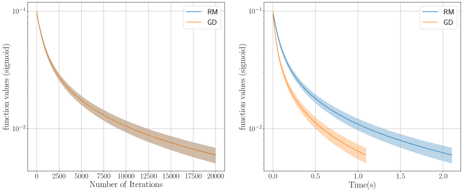
Figure 2: Average of the objective function value with sigmoid link function

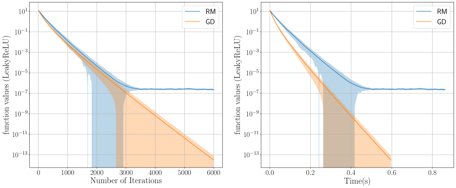
Figure 3: Average of the objective function value with Leaky ReLU link function

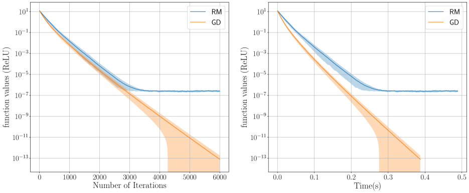
Figure 4: Average of the objective function value with ReLU link function

F.2 Function $\bar{f}_{T,\sigma}$

In Hinder et al. (2020) a function was introduced and proved to be quasar-convex and they named it as “hard function”. It is denoted by $\bar{f}_{T,\sigma}$. Function $\bar{f}_{T,\sigma}\overset{\text{def}}{=}q(x)+\sigma\sum_{i=0}^{T}\Upsilon(x_{i}),$ where $\Upsilon(\theta)\overset{\text{def}}{=}120\int_{1}^{\theta}\frac{t^{2}(t-1)}{1+t^{2}}\mathrm{d}t$ and $q(x)\overset{\text{def}}{=}\frac{1}{4}(x_{1}-1)^{2}+\frac{1}{4}\sum_{i=1}^{T-1}(x_{i}-x_{i+1})^{2}.$ They showed $L_{1}=3$ and $\gamma=\frac{1}{100T\sqrt{\sigma}}$ for this function. We choose $T=20,$ $\sigma=10^{-6},$ $N=50000,$ $h=10^{-3},$ $\mu=10^{-4},$ and the initial point is sampled from $\mathcal{N}(0,I_{T})$. The average of the loss function value and its standard deviation over 10 runs, in both number of iterations and CPU time, are presented for both RM and GD in Figure 5.

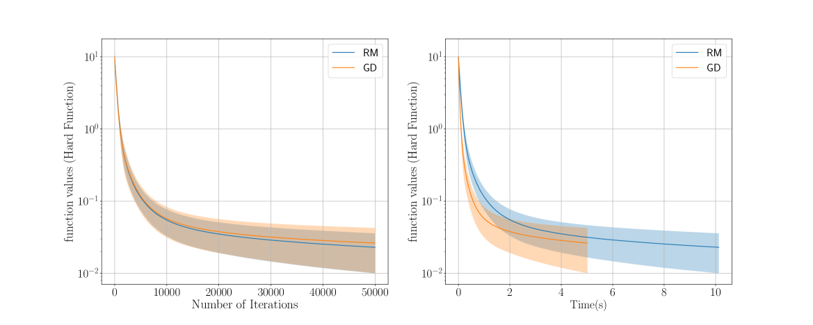
Figure 5: Average of the $\bar{f}_{T,\sigma}$ objective function value

F.3 LDSI

We generate the true parameters and inputs the same way as Hardt et al. (2018) with $n=20$ and $T=500$. Following Hinder et al. (2020), we generate 100 sequences at the beginning and we actually minimise $\frac{1}{|\mathcal{B}|}\sum_{(x,y)\in\mathcal{B}}\big{(}\frac{1}{T-T_{1}}\sum_{i=T_{1}}^{T}(y_{t}-\hat{y}_{t})^{2}\big{)},$ where $\mathcal{B}$ is batch of 100 sequences and $T_{1}\overset{\text{def}}{=}\frac{T}{4}.$ The initial point $(\hat{A}_{0},\hat{C}_{0},\hat{D}_{0})$ by perturbing the true parameters $(A,C,D)$ and considering that the spectral radius of $\hat{A}_{0}$ remains less than $1$. Note that $B$ is known and $\hat{B}=B.$ The quasar-convexity parameter $\gamma$ calculated in Hardt et al. (2018), is difficult to calculate precisely in practice and we simply tune that numerically in the simulations (same happened for $L_{1}(f$)). Following Fu et al. (2023), the random noise $\xi_{t}\sim 10^{-2}\mathcal{N}(0,I_{n})$. We choose $N=1000,$ $h=10^{-5},$ $\mu=10^{-4}$. We note that RM can diverge when $h$ is bigger than this value, but we repeated the experiment using GD with $h=10^{-4}$ too.

F.4 SVM with smoothed hinge loss

This numerical example is explained completely in Section 5.2. The average of the loss function value and its standard deviation, for $h=10^{-4}$, in both number of iterations and CPU time, are presented Figure 6.

Figure 6: Average of the SVM objective function value

F.5 Entropy Regularised Policy gradient Reinforcement Learning

In this subsection, we evaluate Algorithm 1 on entropy regularised RL. It is shown in (Mei et al., 2020, Lemma 15) that the problem satisfies the PL inequality and has Lipschitz gradients. It is known that a PL function, which is quasar-convex, is strongly-quasar convex. Following the example in (Mei et al., 2020, Appendix D.2), we choose one state (bandit case) and $20$ actions. The reward ($r(a)\in[0,1]$) is chosen randomly, initial $\theta$ is sampled randomly from the Gaussian distribution, the step size is set to $0.1$, and $\mu=10^{-5}$. See more details and complete formulation in (Mei et al., 2020, Section 2 and 4)). The loss function is $\underset{{\theta}}{\max}\underset{a\sim\pi_{\theta}}{\mathbb{E}}[r(a)-\tau\log(\pi_{\theta}(a))]$ and the convergence criteria is soft sub-optimality error ($\delta_{t}={\pi_{\tau}^{\ast}}^{T}(r-\tau\log(\pi_{\tau}^{\ast})))-\pi_{\theta_{t}}^{T}(t-\tau\log(\pi_{\theta_{t}}))$). Figure 7 depicts the average of soft sub-optimality error over 20 runs, for $\tau=0.5$ and $\tau=5$. Similarly as Cen et al. (2022), it can be seen that by increasing $\tau$ the final $\delta_{t}$ gets smaller and the convergence is faster.

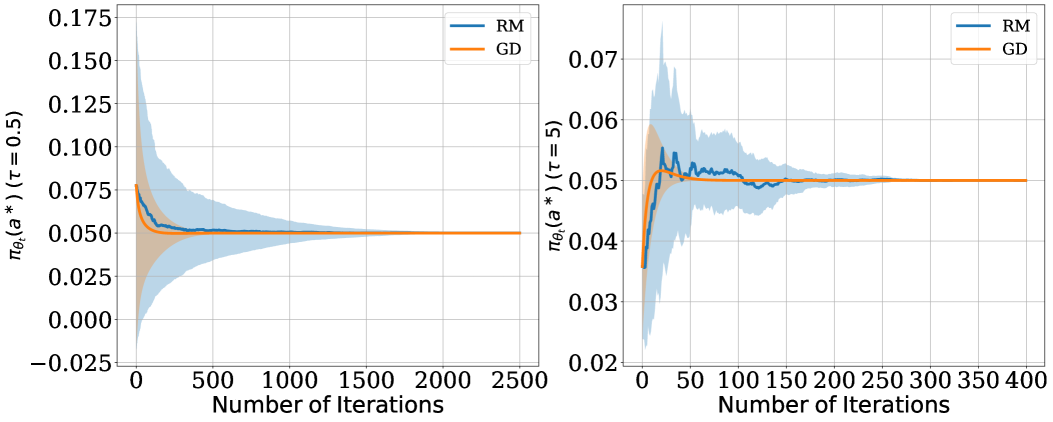
Figure 7: The soft sub-optimality error value

F.6 Recurrent Neural Network with Residues

In this section we evaluate the performance of Algorithm 1 on a deep network with one hidden layer. The formulation of recurrent neural networks with linear activation functions are very similar to what we have in previous experiment. The structure of the evaluated network is shown in Figure 8. We are given observations ${(x_{t},y_{t})}_{i=1}^{T}\in\mathbb{R}\times\mathbb{R}$ and the predicted output will be obtained using $h_{t+1}=\Gamma(Ah_{t}+Bx_{t});\;\hat{y}_{t}=Ch_{t}+Dx_{t},$ where $\Gamma(.)$ is the activation function, $h_{t}\in\mathbb{R}^{n}$ is the hidden state at time $t,$ and accordingly $A\in\mathbb{R}^{n\times n},$ $B\in\mathbb{R}^{n\times 1},$ $C\in\mathbb{R}^{1\times n},$ $D\in\mathbb{R}.$ We seek to learn the unknown weights ($A,B,C,D$) by minimising the well known loss function : $\frac{1}{T}\sum_{i=1}^{T}(y_{t}-\hat{y}_{t})^{2}.$ We choose $n=20$ (number of cells in the hidden layer), $T=100$(length of the input sequence), and generate 500 samples (sequences with length $T$ and their target) which are randomly sampled from zero mean unit variance Normal distribution. The sigmoid function is used as the activation layer($\Gamma(.)$). We choose to have a full batch approach and actually minimise $\frac{1}{|\mathcal{B}|}\sum_{(x,y)\in\mathcal{B}}\big{(}\frac{1}{T-T_{1}}\sum_{i=T_{1}}^{T}(y_{t}-\hat{y}_{t})^{2}\big{)},$ where $\mathcal{B}$ is batch of 500 sequences and $T_{1}\overset{\text{def}}{=}\frac{T}{10}.$ The initial weights are randomly sampled from zero mean unit variance Normal distribution too. The other parameters are tuned numerically and $N=1000,$ $h=10^{-4},$ $\mu=10^{-4}$. Note that while it this structure is not shown to satisfy any particular property, in Hardt & Ma (2017), it is established that linear residual networks (along with certain assumptions) satisfy the PL condition. In light of Lemma 8, and knowing the properties of the aforementioned linear dynamical system, even-though this network is not linear, we decided to evaluate the algorithm on this task as well. One can see the average of the objective function value and its standard deviation over 3 runs in both number of iterations and CPU time, for both RM and GD, in Figure 9. it can be seen that Algorithm 1 performs better than GD in this example.

Figure 8: Structure of the trained deep network

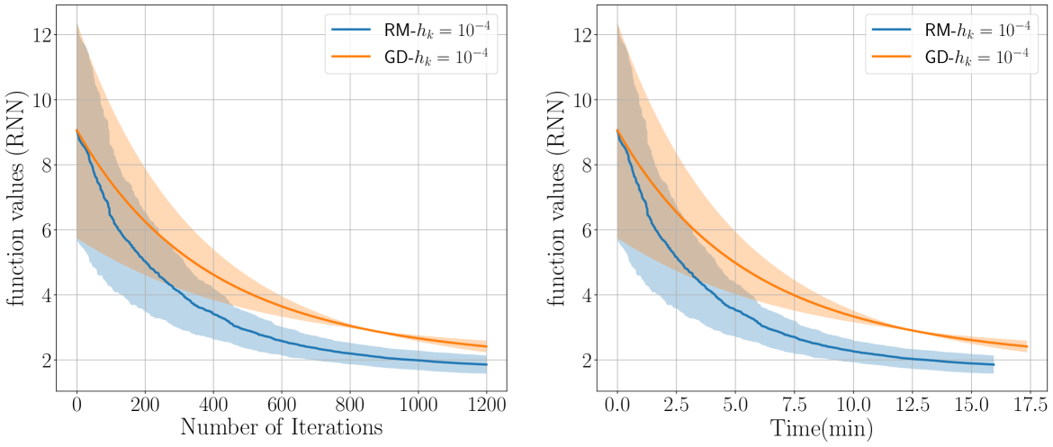
Figure 9: Average of the RNN objective function value

References

- Anagnostidis et al. (2021) Sotirios-Konstantinos Anagnostidis, Aurelien Lucchi, and Youssef Diouane. Direct-search for a class of stochastic min-max problems. In International Conference on Artificial Intelligence and Statistics, pp. 3772–3780. PMLR, 2021.
- Audet & Hare (2017) Charles Audet and Warren Hare. Introduction: tools and challenges in derivative-free and blackbox optimization. Springer, 2017.
- Balasubramanian & Ghadimi (2022) Krishnakumar Balasubramanian and Saeed Ghadimi. Zeroth-order nonconvex stochastic optimization: Handling constraints, high dimensionality, and saddle points. Foundations of Computational Mathematics, 22(1):35–76, 2022.
- Bengio et al. (1994) Yoshua Bengio, Patrice Simard, and Paolo Frasconi. Learning long-term dependencies with gradient descent is difficult. IEEE transactions on neural networks, 5(2):157–166, 1994.
- Cartis et al. (2010) Coralia Cartis, Nicholas IM Gould, and Ph L Toint. On the complexity of steepest descent, newton’s and regularized newton’s methods for nonconvex unconstrained optimization problems. Siam journal on optimization, 20(6):2833–2852, 2010.
- Cen et al. (2022) Shicong Cen, Chen Cheng, Yuxin Chen, Yuting Wei, and Yuejie Chi. Fast global convergence of natural policy gradient methods with entropy regularization. Operations Research, 70(4):2563–2578, 2022.
- Chen et al. (2024) Aochuan Chen, Yimeng Zhang, Jinghan Jia, James Diffenderfer, Konstantinos Parasyris, Jiancheng Liu, Yihua Zhang, Zheng Zhang, Bhavya Kailkhura, and Sijia Liu. Deepzero: Scaling up zeroth-order optimization for deep model training. In ICLR, 2024.
- Dua & Graff (2019) Dheeru Dua and Casey Graff. Uci machine learning repository, 2019. URL http://archive.ics.uci.edu/ml.
- Farzin & Shames (2024) Amir Ali Farzin and Iman Shames. Minimisation of polyak-Łojasewicz functions using random zeroth-order oracles. In 2024 European Control Conference (ECC), pp. 3207–3212, 2024. doi: 10.23919/ECC64448.2024.10590822.
- Farzin et al. (2025) Amir Ali Farzin, Yuen Man Pun, Philipp Braun, Antoine Lesage-landry, Youssef Diouane, and Iman Shames. Min-max optimisation for nonconvex-nonconcave functions using a random zeroth-order extragradient algorithm. arXiv preprint arXiv:2504.07388, 2025.
- Fu et al. (2023) Qiang Fu, Dongchu Xu, and Ashia Camage Wilson. Accelerated stochastic optimization methods under quasar-convexity. In International Conference on Machine Learning, pp. 10431–10460. PMLR, 2023.
- Ghadimi et al. (2016) Saeed Ghadimi, Guanghui Lan, and Hongchao Zhang. Mini-batch stochastic approximation methods for nonconvex stochastic composite optimization. Mathematical Programming, 155(1-2):267–305, 2016.
- Goodfellow et al. (2014) Ian J Goodfellow, Jonathon Shlens, and Christian Szegedy. Explaining and harnessing adversarial examples. arXiv preprint arXiv:1412.6572, 2014.
- Guminov et al. (2017) Sergey Guminov, Alexander Gasnikov, and Ilya Kuruzov. Accelerated methods for -weakly-quasi-convex problems. arXiv preprint arXiv:1710.00797, 2017.
- Hardt & Ma (2017) Moritz Hardt and Tengyu Ma. Identity matters in deep learning. In International Conference on Learning Representations, 2017.
- Hardt et al. (2018) Moritz Hardt, Tengyu Ma, and Benjamin Recht. Gradient descent learns linear dynamical systems. Journal of Machine Learning Research, 19(29):1–44, 2018.
- Hinder et al. (2020) Oliver Hinder, Aaron Sidford, and Nimit Sohoni. Near-optimal methods for minimizing star-convex functions and beyond. In Conference on learning theory, pp. 1894–1938. PMLR, 2020.
- Huang et al. (2022) Feihu Huang, Shangqian Gao, Jian Pei, and Heng Huang. Accelerated zeroth-order and first-order momentum methods from mini to minimax optimization. Journal of Machine Learning Research, 23(36):1–70, 2022.
- Jin (2020) Jikai Jin. On the convergence of first order methods for quasar-convex optimization. arXiv preprint arXiv:2010.04937, 2020.
- Karimi et al. (2016) Hamed Karimi, Julie Nutini, and Mark Schmidt. Linear convergence of gradient and proximal-gradient methods under the polyak-łojasiewicz condition. In Machine Learning and Knowledge Discovery in Databases: European Conference, ECML PKDD 2016, Riva del Garda, Italy, September 19-23, 2016, Proceedings, Part I 16, pp. 795–811. Springer, 2016.
- Lin et al. (2024) Zhanran Lin, Puheng Li, and Lei Wu. Exploring neural network landscapes: Star-shaped and geodesic connectivity. arXiv preprint arXiv:2404.06391, 2024.
- Liu et al. (2018) Sijia Liu, Bhavya Kailkhura, Pin-Yu Chen, Paishun Ting, Shiyu Chang, and Lisa Amini. Zeroth-order stochastic variance reduction for nonconvex optimization. Advances in Neural Information Processing Systems, 31, 2018.
- Liu et al. (2020a) Sijia Liu, Songtao Lu, Xiangyi Chen, Yao Feng, Kaidi Xu, Abdullah Al-Dujaili, Mingyi Hong, and Una-May O’Reilly. Min-max optimization without gradients: Convergence and applications to black-box evasion and poisoning attacks. In International Conference on Machine Learning, pp. 6282–6293. PMLR, 2020a.
- Liu et al. (2020b) Sijia Liu, Parikshit Ram, Deepak Vijaykeerthy, Djallel Bouneffouf, Gregory Bramble, Horst Samulowitz, Dakuo Wang, Andrew Conn, and Alexander Gray. An admm based framework for automl pipeline configuration. In Proceedings of the AAAI Conference on Artificial Intelligence, volume 34, pp. 4892–4899, 2020b.
- Maass et al. (2021) Alejandro I Maass, Chris Manzie, Iman Shames, and Hayato Nakada. Zeroth-order optimization on subsets of symmetric matrices with application to mpc tuning. IEEE Transactions on Control Systems Technology, 30(4):1654–1667, 2021.
- Mei et al. (2020) Jincheng Mei, Chenjun Xiao, Csaba Szepesvari, and Dale Schuurmans. On the global convergence rates of softmax policy gradient methods. In International conference on machine learning, pp. 6820–6829. PMLR, 2020.
- Moriarty et al. (1999) David E Moriarty, Alan C Schultz, and John J Grefenstette. Evolutionary algorithms for reinforcement learning. Journal of Artificial Intelligence Research, 11:241–276, 1999.