Hyper Boris integrators for kinetic plasma simulations

Abstract

We propose a family of numerical solvers for the nonrelativistic Newton–Lorentz equation in kinetic plasma simulations. The new solvers extend the standard 4-step Boris procedure, which has second-order accuracy in time, in three ways. First, we repeat the 4-step procedure multiple times, using an $n$-times smaller timestep ($\Delta t/n$). We derive a formula for the arbitrary subcycling number $n$, so that we obtain the result without repeating the same calculations. Second, prior to the 4-step procedure, we apply Boris-type gyrophase corrections to the electromagnetic field. In addition to a well-known correction to the magnetic field, we correct the electric field in an anisotropic manner to achieve higher-order ($N=2,4,6\dots$th order) accuracy. Third, combining these two methods, we propose a family of high-accuracy particle solvers, the hyper Boris solvers, which have two hyperparameters of the subcycling number $n$ and the order of accuracy, $N$. The $n$-cycle $N$th-order solver gives a numerical error of $\sim(\Delta t/n)^{N}$ at affordable computational cost.

1 Introduction

Kinetic plasma simulations such as particle-in-cell (PIC) simulation [8, 3, 18] and hybrid simulation [11] are very useful for understanding complex phenomena in space, solar, and astrophysical plasmas. These simulations resolve Lagrange motions of many charged particles, typically $10^{2}$–$10^{3}$ particles in a grid cell, and $10^{8}$–$10^{12}$ particles in the entire simulation domain. Even though they are computationally very expensive, kinetic simulations are capable of reproducing various kinetic processes from the first principle.

One of the most important components of kinetic plasma simulations is a particle integrator, also referred to as a particle pusher, which advances individual particles in the electromagnetic field by using the Newton–Lorentz equation. One of the most popular particle integrators is the Boris solver [4], or the so-called Buneman–Boris solver. The Boris solver is relatively simple, consists of four-step operations as will be shown in this paper, and it is proven to preserve the phase-space volume [14]. The solver has a second-order accuracy in time, i.e., it produces an error $\propto(\Delta t)^{2}$ in velocity, where $\Delta t$ is the timestep. Owing to its simplicity, numerical stability, and good accuracy, it has been used as the de facto standard method for over a half century.

Since there is always a demand for better simulation results, scientists have been actively developing high-accuracy integrators [13, 7, 19, 16, 17, 21, 22, 12]. In addition, modern processors are so fast that the data transfer inside the chip or from the memory often becomes a bottleneck for simulations. In such a case, even though computationally expensive, higher-order or higher-accuracy integrators that provide good results without extra data transfer are favorable. Nevertheless, most of the current integrators have second-order accuracy, and they do not drastically outperform the second-order Boris solver. The number of higher-order particle integrators is still limited [19].

In this study, we propose a new family of high-accuracy Boris-type integrators for nonrelativistic kinetic simulations. Three enhancements to the standard Boris solver are presented. In Section 2, we briefly review basic issues. We outline the standard Boris solver and its gyrophase correction in Section 2.1, and the multiple Boris solver [22] which subcycles the Lorentz-force part of the Newton–Lorentz equation in Section 2.2. In Section 3, we propose a new subcycling method that repeats the entire 4-step procedure. In Section 4, we propose higher-order corrections to the 4-step Boris solver. In Section 5, combining the two methods, we propose a family of high-accuracy particle solvers, the hyper Boris solvers. It has two hyperparameters of the subcycling number $n$ and the order of accuracy, $N$. Section 6 presents numerical tests of the proposed methods. Section 7 contains discussion and summary.

2 Review

2.1 Boris solver

Here we discuss a popular implementation of the Boris solver [4]. We limit our attention to the nonrelativistic particle motion. We use SI units. We consider the equation of motion in a leap-frog and discrete manner,

$$\frac{\bm{x}^{t+\Delta t/2}-\bm{x}^{t-\Delta t/2}}{\Delta t} =\bm{v}^{t}$$ (1)

$$\frac{\bm{v}^{t+\Delta t}-\bm{v}^{t}}{\Delta t} =\frac{q}{m}\left(\bm{E}^{t+\frac{\Delta t}{2}}+\frac{{\bm{v}^{t+\Delta t}+\bm{v}^{t}}}{2}\times\bm{B}^{t+\frac{\Delta t}{2}}\right)$$ (2)

where $\bm{x}$ is the position, $\bm{v}$ is the velocity, $q$ is the charge, $m$ is the mass of the particle, $\bm{E}$ is the electric field at the particle position, $\bm{B}$ is the magnetic field, and $\Delta t$ is the timestep. The superscript indicates the time, i.e., $\bm{v}^{t}$ is the velocity of the particle at time $t$. The electromagnetic fields are customarily assumed uniform and stationary from $t$ and $t+\Delta t$, and we drop the superscripts from $\bm{E}$ and $\bm{B}$ for simplicity. We further define the element magnetic/electric vectors,

$$\bm{\tau}_{1} \equiv\frac{q\Delta t}{2m}\bm{B},~~~\bm{\varepsilon}_{1}\equiv\frac{q\Delta t}{2m}\bm{E}$$ (3)

These vectors are basic elements of numerical procedures in this paper. Eq. (2) approximates an exact solution for the next velocity $\bm{v}^{t+\Delta t}$,

$$\bm{v}^{t+\Delta t} =\cos(2\tau_{1})\bm{v}^{t}+2{\rm sinc}(2\tau_{1})(\bm{v}^{t}\times\bm{\tau}_{1}+\bm{\varepsilon}_{1})$$

$$~~~+2{\rm sinc}^{2}(\tau_{1})\Big{(}(\bm{v}^{t}\cdot\bm{\tau}_{1})\bm{\tau}_{1}+\bm{\varepsilon}_{1}\times\bm{\tau}_{1}\Big{)}+\frac{2(1-{\rm sinc}(2\tau_{1}))}{\tau_{1}^{2}}(\bm{\varepsilon}\cdot\bm{\tau}_{1})\bm{\tau}_{1},$$ (4)

where ${\rm sinc}(x)\equiv\sin(x)/x$ is the sinc function and $\tau_{1}=|\bm{\tau}_{1}|$. For reference, Eq. (4) is derived in A. When $\tau_{1}=0$, Eq. (4) contains divisions by zero inside the sinc function and in the coefficient of the last term, and therefore the equation is not convenient for numerical calculation.

The Boris solver gives a second-order approximation of Eq. (4). We tentatively set $\bm{t}_{1}=\bm{\tau}_{1}$ and $\bm{e}_{1}=\bm{\varepsilon}_{1}$. It accelerates the particle velocity by the following 4 steps.

$$\left\{\begin{array}[]{ll}\bm{v}^{-}&=\bm{v}^{t}+\bm{e}_{1}\\ \bm{v}^{{}^{\prime}}&=\bm{v}^{-}+\bm{v}^{-}\times\bm{t}_{1}\\ \bm{v}^{+}&=\bm{v}^{-}+\dfrac{2}{1+t_{1}^{2}}~\bm{v}^{{}^{\prime}}\times\bm{t}_{1}\\ \bm{v}^{t+\Delta t}&=\bm{v}^{+}+\bm{e}_{1}\end{array}\right.$$ (9)

Here, $\bm{v}^{+},\bm{v}^{-},\bm{v}^{\prime}$ are intermediate velocities. The first and fourth equations represent the half-acceleration by $\bm{E}$, and the second and third equations stand for the gyration about $\bm{B}$. The gyration part is schematically illustrated by the gray dashed lines in Fig. 1(a). One can see that the gyration, the circular motion in the velocity space, is approximated by a combination of two triangles. The phase angle $\theta$ is approximated by

$$\theta=\dfrac{qB}{m}\Delta t=2\tau_{1}\approx 2\alpha_{1}\equiv 2\arctan\tau_{1}$$ (10)

where $\alpha_{1}=\arctan\tau_{1}$ is a half angle of the approximated gyration. Examining the tangent vector from $\bm{v}^{-}$ to $\bm{v}^{\prime}$, one can see the ratio between the true tangent to the approximation is

$$f(\tau_{1})=\frac{\tan\tau_{1}}{\tau_{1}}=1+\frac{1}{3}\tau_{1}^{2}+\frac{2}{15}\tau_{1}^{4}+\frac{17}{315}\tau_{1}^{6}+\dots$$ (11)

This indicates that there is a second-order error in the tangent line and in other places accordingly. The second-order error is usually small, and therefore the 4-step procedure (Eq. (9)) is widely used. We call the 4-step procedure the standard Boris solver (This corresponds to the Boris-B solver in Zenitani & Umeda [21]).

To cancel this error (Eq. (11)), Boris [4] amplified the element magnetic vector by a factor of $f_{N}=f_{N}({\tau}_{1})$, taken from the Taylor expansion up to the $(N-2)$th order ($N=2,4,6,\dots$). For example, for $N=6$,

$$\bm{t}_{1}\equiv f_{6}(\tau_{1})\bm{\tau_{1}}=\left(1+\frac{1}{3}\tau_{1}^{2}+\frac{2}{15}\tau_{1}^{4}\right)\bm{\tau_{1}}$$ (12)

Using this $\bm{t}_{1}$, we use the standard 4-step procedure. Then we can improve the gyration part to the $N$th-order accuracy: $2\alpha_{\rm 1,corr}=\theta+\mathcal{O}(\tau_{1}^{N})$, where the subscript ${\rm corr}$ indicates the corrected value. The corrected gyration is illustrated by the gray solid lines in Fig. 1(a). This correction is known as the gyrophase correction. Note that we only amplifies the magnetic vector $\bm{\tau_{1}}$ for advancing an individual particle. We do not amplify the magnetic field $\bm{B}^{t+\frac{\Delta t}{2}}$ to calculate the fields at the next timestep $\bm{B}^{t+\frac{3\Delta t}{2}}$ and $\bm{E}^{t+\frac{3\Delta t}{2}}$. We call the entire procedure the Boris solver with gyrophase correction (the Boris-A solver in Ref. [21]).

The gyrophase correction allows us to solve the gyration part to a higher-order of accuracy; however, the solver consists of the gyration part and the half-acceleration parts by the electric field. Unless $\bm{E}=0$, the entire 4-step procedure falls back to a second-order accuracy [21]. For this reason, the standard Boris solver without the gyrophase correction is popularly used.

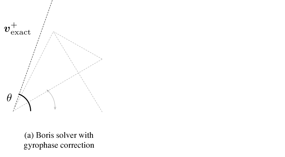
Figure 1: (a) Schematic diagram of the Lorentz-force part of the Boris solver with gyrophase correction. The subscript ‘corr’ emphasizes a corrected value. (b) The Lorentz-force part of the multiple Boris solver [22] with $n=2$.

2.2 Multiple Boris solver

Next, we outline the multiple Boris solver [22], which subcycles the gyration part of the Boris solver. The middle two procedures in Eq. (9) that advance the pre-gyration state $\bm{v}^{-}$ to the post-gyration state $\bm{v}^{+}$ are repeated $n$ times with a $n$-times smaller timestep, $\Delta t/n$. The gyration part of the $n=2$ case is illustrated in Figure 1(b). Here, we use the element magnetic vector $\bm{t}_{n}$ and the relevant half angle $\alpha_{n}$,

$$\bm{t}_{n}\equiv\bm{\tau}_{n}\equiv\frac{\bm{\tau}_{1}}{n},~~\alpha_{n}\equiv\arctan t_{n}.$$ (13)

Zenitani & Kato [22] have derived the post-gyration state $\bm{v}^{+}$ of the multiple Boris solver for an arbitrary positive integer $n$.

$$\bm{v}^{+} =c_{n1}\bm{v}^{-}+c_{n2}~(\bm{v}^{-}\times\bm{t}_{n})+c_{n3}(\bm{v}^{-}\cdot\bm{t}_{n})\bm{t}_{n}$$ (14)

where $c_{n1}$, $c_{n2}$, and $c_{n3}$ are the following coefficients,

$$c_{n1} =\cos(2n\alpha_{n})=T_{n}(p_{n})$$ (15)

$$c_{n2} =\cfrac{\sin(2n\alpha_{n})}{t_{n}}=\frac{2}{1+t_{n}^{2}}U_{n-1}(p_{n})$$ (16)

$$c_{n3} =\cfrac{1-\cos(2n\alpha_{n})}{t_{n}^{2}}=\left\{\begin{array}[]{ll}\dfrac{2}{1+t_{n}^{2}}&{\rm(for~{\it n}=1)}\\ \dfrac{2}{1+t_{n}^{2}}\Big{(}U_{k}(p_{n})+U_{k-1}(p_{n})\Big{)}^{2}&{\rm(for~{\it n}=2k+1)}\\ \dfrac{8}{(1+t_{n}^{2})^{2}}\Big{(}U_{k-1}\big{(}p_{n})\Big{)}^{2}&{\rm(for~{\it n}=2k)}\end{array}\right.$$ (20)

where $T_{n}(x)$ and $U_{n}(x)$ are Chebyshev polynomials of the first kind and the second kind, $k$ in Eq. (20) is a positive integer, and $p_{n}$ is the cosine parameter,

$$p_{n}\equiv\cos 2\alpha_{n}=\frac{1-t_{n}^{2}}{1+t_{n}^{2}}.$$ (21)

Importantly, by using Eq. (14), we can immediately obtain the post-gyration state $\bm{v}^{+}$ without repeating the 2-step calculation $n$ times. The numerical error of the gyration part is $\propto(\Delta t/n)^{2}$, as expected [22].

3 Multicycle solver

Motivated by the multiple Boris solver, we propose to subcycle the entire 4-step procedure of the particle integrator. We call this method the multicycle method. Note that the multiple Boris solver subcycles the Lorentz-force part inside the 4-step procedure, but the multicycle solver subcycles the entire 4-step procedure.

We first define

$$\bm{t}_{n}\equiv\bm{\tau}_{n}\equiv\frac{\bm{\tau}_{1}}{n},~~\bm{e}_{n}\equiv\bm{\varepsilon}_{n}\equiv\frac{\bm{\varepsilon}_{1}}{n},~~\alpha_{n}\equiv\arctan t_{n},$$ (22)

We rewrite $\bm{v}^{(0)}=\bm{v}^{t}$, $\bm{v}^{(n)}=\bm{v}^{t+\Delta t}$, and the intermediate states $\bm{v}^{(1)},\bm{v}^{(2)},\cdots,\bm{v}^{(n-1)}$. Each subcycle advances $\bm{v}^{(k)}$ to $\bm{v}^{(k+1)}$. The entire procedure is equivalent to

$$\left.\begin{array}[]{c}\left\{\begin{array}[]{ll}\bm{v}^{-}&=\bm{v}^{(0)}+\bm{e}_{n}\\ \bm{v}^{+}&=\mathbb{R}_{\bm{b}}(2\alpha_{n})~\bm{v}^{-}\\ \bm{v}^{(1)}&=\bm{v}^{+}+\bm{e}_{n}\end{array}\right.\\ \vdots\\ \left\{\begin{array}[]{ll}\bm{v}^{-}&=\bm{v}^{(n-1)}+\bm{e}_{n}\\ \bm{v}^{+}&=\mathbb{R}_{\bm{b}}(2\alpha_{n})~\bm{v}^{-}\\ \bm{v}^{(n)}&=\bm{v}^{+}+\bm{e}_{n}\end{array}\right.\end{array}~~~~~~~\right\}\times~n~{\rm cycles}$$ (32)

Here we express the 4-step procedure in three lines. The gyration part is rewritten by a rotation operator $\mathbb{R}_{\bm{b}}(2\alpha_{n})$ on the pre-gyration state $\bm{v}^{-}$. It stands for a rotation about the $\bm{b}\equiv\bm{B}/|B|$ axis with a rotation angle $2\alpha_{n}$.

After $n$ cycles, the result of Eq. (32) is given by

$$\bm{v}^{(n)} =\mathbb{R}_{\bm{b}}(2n\alpha_{n})~\bm{v}^{(0)}+\bigg{(}\mathbb{R}_{\bm{b}}(2n\alpha_{n})+2\sum_{j=1}^{n-1}\mathbb{R}_{\bm{b}}(2j\alpha_{n})+\mathbb{I}\bigg{)}~\bm{e}_{n}$$

$$=\mathbb{R}_{\bm{b}}(2n\alpha_{n})~\bm{v}^{(0)}+\sum_{j=0}^{n-1}\bigg{(}\mathbb{R}_{\bm{b}}(2(j+1)\alpha_{n})+\mathbb{R}_{\bm{b}}(2j\alpha_{n})\bigg{)}~\bm{e}_{n}.$$ (33)

In the multiple Boris solver (Sec. 2.2), we notice that the post-gyration vector $\bm{v}^{+}$ is rotated from $\bm{v}^{-}$ with an angle $2\alpha_{n}$. Then we can apply the multi-Boris formula (Eq. (14)) to the first term of the right hand side of Eq. (33),

$$\mathbb{R}_{\bm{b}}(2n\alpha_{n})~\bm{v}^{(0)} =c_{n1}\bm{v}^{(0)}+c_{n2}~(\bm{v}^{(0)}\times\bm{t}_{n})+c_{n3}(\bm{v}^{(0)}\cdot\bm{t}_{n})\bm{t}_{n}$$ (34)

The coefficients $c_{n1},c_{n2},c_{n3}$ are given by Eqs. (15)–(20). We similarly apply the formula to the second term of the right hand side of Eq. (33), and then obtain

$$\sum_{j=0}^{n-1}\bigg{(}\mathbb{R}_{\bm{b}}(2(j+1)\alpha_{n})+\mathbb{R}_{\bm{b}}(2j\alpha_{n})\bigg{)}~\bm{e}_{n}~~~~~~~~~~~~~~~~~~~~~~~~~$$

$$~~~~=\Big{(}\sum_{j=0}^{n-1}\left(c_{j+1,1}+c_{j1}\right)\Big{)}\bm{e}_{n}+\Big{(}\sum_{j=0}^{n-1}\left(c_{j+1,2}+c_{j2}\right)\Big{)}(\bm{e}_{n}\times\bm{t}_{n})+\Big{(}\sum_{j=0}^{n-1}\left(c_{j+1,3}+c_{j3}\right)\Big{)}(\bm{e}_{n}\cdot\bm{t}_{n})\bm{t}_{n},$$ (35)

where $c_{n1},c_{n2},c_{n3}$ are the coefficients by Eqs. (15)–(20). We further examine the terms in the right hand side of Eq. (35). Using Eqs. (15) and (16), we find

$$\sum_{j=0}^{n-1}\left(c_{j+1,1}+c_{j1}\right) =\frac{\sin\alpha_{n}}{\sin\alpha_{n}}\cdot\sum_{j=0}^{n-1}\Big{(}\cos(2j+2)\alpha_{n}+\cos 2j\alpha_{n}\Big{)}$$

$$=\frac{\cos\alpha_{n}}{\sin\alpha_{n}}\cdot\sum_{j=0}^{n-1}\Big{(}\sin(2j+2)\alpha_{n}-\sin 2j\alpha_{n}\Big{)}$$

$$=\frac{\sin 2n\alpha_{n}}{t_{n}}=c_{n2}.$$ (36)

Using Eqs. (15)–(20), we similarly find

$$\sum_{j=0}^{n-1}\left(c_{j+1,2}+c_{j2}\right) =\frac{\sin\alpha_{n}}{\sin\alpha_{n}}\cdot\frac{1}{t_{n}}\sum_{j=0}^{n-1}\Big{(}\sin(2j+2)\alpha_{n}+\sin 2j\alpha_{n}\Big{)}$$

$$=-\frac{\cos\alpha_{n}}{\sin\alpha_{n}}\cdot\frac{1}{t_{n}}\sum_{j=0}^{n-1}\Big{(}\cos(2j+2)\alpha_{n}-\cos 2j\alpha_{n}\Big{)}$$

$$=\frac{1-\cos 2n\alpha_{n}}{t^{2}_{n}}=c_{n3}.$$ (37)

Using Eqs. (15)–(20) and (36), we obtain

$$\sum_{j=0}^{n-1}\left(c_{j+1,3}+c_{j3}\right) =\frac{1}{t_{n}^{2}}\left(2n-\sum_{j=0}^{n-1}\left(c_{j+1,1}+c_{j1}\right)\right)=\frac{2n-c_{n2}}{t_{n}^{2}}=\frac{2}{t_{n}^{2}}\bigg{(}n-\frac{1}{1+t_{n}^{2}}U_{n-1}(p_{n})\bigg{)}$$ (38)

Summarizing Eqs. (33)–(38) and recovering the original notation of $\bm{v}^{t+\Delta t}$ and $\bm{v}^{t}$, we obtain the following form

$$\bm{v}^{t+\Delta t} =c_{n1}\bm{v}^{t}+c_{n2}~(\bm{v}^{t}\times\bm{t}_{n})+c_{n3}(\bm{v}^{t}\cdot\bm{t}_{n})\bm{t}_{n}+c_{n4}\bm{e}_{n}+c_{n5}(\bm{e}_{n}\times\bm{t}_{n})+c_{n6}(\bm{e}_{n}\cdot\bm{t}_{n})\bm{t}_{n}$$ (39)

where we use the following coefficients, $c_{n1}\dots c_{n6}$. The first three coefficients and the cosine parameter $p_{n}$ are identical to ones in Section 2.2, but we show them here for completeness.

$$c_{n1} =T_{n}\left(p_{n}\right)$$ (40)

$$c_{n2} =c_{n4}=\frac{2}{1+t_{n}^{2}}U_{n-1}\left(p_{n}\right)$$ (41)

$$c_{n3} =c_{n5}=\left\{\begin{array}[]{ll}\dfrac{2}{1+t_{n}^{2}}&{\rm(for~{\it n}=1)}\\ \dfrac{2}{1+t_{n}^{2}}\left(U_{k}\left(p_{n}\right)+U_{k-1}\left(p_{n}\right)\right)^{2}&{\rm(for~{\it n}=2k+1)}\\ \dfrac{8}{(1+t_{n}^{2})^{2}}\left(U_{k-1}\left(p_{n}\right)\right)^{2}&{\rm(for~{\it n}=2k)}\end{array}\right.$$ (45)

$$c_{n6} =\frac{2}{t_{n}^{2}}\left(n-\frac{1}{1+t_{n}^{2}}U_{n-1}\left(p_{n}\right)\right)$$ (46)

$$p_{n} =\frac{1-t_{n}^{2}}{1+t_{n}^{2}}$$ (47)

The multicycle formula (Eq. (39)) holds true, even for $\bm{t}_{n}=0$. In practice, we can just use Eq. (39) to obtain $\bm{v}^{t+\Delta t}$. This is much quicker than repeating the 4-step procedure $n$ times.

The new solver will be tested in Section 6. For reference, we list some coefficients here ($n=1,2,4$).

$$c_{11}=\frac{1-t_{1}^{2}}{1+t_{1}^{2}},~~c_{12}=c_{13}=c_{14}=c_{15}=c_{16}=\frac{2}{1+t_{1}^{2}},$$ (48)

$$c_{21}=\frac{1-6t_{2}^{2}+t_{2}^{4}}{(1+t_{2}^{2})^{2}},~~c_{22}=c_{24}=\frac{4(1-t_{2}^{2})}{(1+t_{2}^{2})^{2}},~~c_{23}=c_{25}=\frac{8}{(1+t_{2}^{2})^{2}},~~c_{26}=\frac{4(3+t_{2}^{2})}{(1+t_{2}^{2})^{2}},$$ (49)

$$c_{41}=\frac{1-28t_{4}^{2}+70t_{4}^{4}-28t_{4}^{6}+t_{4}^{8}}{(1+t_{4}^{2})^{4}},~~c_{42}=c_{44}=\frac{8(1-7t_{4}^{2}+7t_{4}^{4}-t_{4}^{6})}{(1+t_{4}^{2})^{4}},~~$$

$$c_{43}=c_{45}=\frac{32(1-t_{4}^{2})^{2}}{(1+t_{4}^{2})^{4}},~~c_{46}=\frac{8(11-t_{4}^{2}+5t_{4}^{4}+t_{4}^{6})}{(1+t_{4}^{2})^{4}}$$ (50)

4 Higher-order correction

In this section, we develop a higher-order correction. We consider the standard Boris solver without gyrophase correction. We retain $\bm{t}_{1}\equiv\bm{\tau}_{1}$ and $\bm{e}_{1}\equiv\bm{\varepsilon}_{1}$. Substituting $n=1$ into Eq. (39), we rewrite the 4-step procedure (Eq. (9))

$$\bm{v}^{t+\Delta t} =\frac{1-t_{1}^{2}}{1+t_{1}^{2}}\bm{v}^{t}+\frac{2}{1+t_{1}^{2}}\bm{v}^{t}\times\bm{t}_{1}+\frac{2}{1+t_{1}^{2}}\left(\bm{v}^{t}\cdot\bm{t}_{1}\right)\bm{t}_{1}$$

$$~~~+\frac{2}{1+t_{1}^{2}}\bm{e}_{1}+\frac{2}{1+t_{1}^{2}}\bm{e}_{1}\times\bm{t}_{1}+\frac{2}{1+t_{1}^{2}}(\bm{e}_{1}\cdot\bm{t}_{1})\bm{t}_{1}$$ (51)

For a moment we assume $|\bm{t}_{1}|\neq 0$. We rewrite the fourth term of the right hand side, by using a vector triplet $-(\bm{e}_{1}\times\bm{t}_{1})\times\bm{t}_{1}=t_{1}^{2}\bm{e}_{1}-{(\bm{e}_{1}\cdot\bm{t}_{1})\bm{t}_{1}}$,

$$\bm{v}^{t+\Delta t} =\frac{1-t_{1}^{2}}{1+t_{1}^{2}}\bm{v}^{t}+\frac{2}{1+t_{1}^{2}}\bm{v}^{t}\times\bm{t}_{1}+\frac{2}{1+t_{1}^{2}}\left(\bm{v}^{t}\cdot\bm{t}_{1}\right)\bm{t}_{1}$$

$$~~~+\frac{2}{1+t_{1}^{2}}\bm{e}_{1}\times\bm{t}_{1}-\frac{2}{1+t_{1}^{2}}\frac{(\bm{e}_{1}\times\bm{t}_{1})}{t_{1}^{2}}\times\bm{t}_{1}+2\frac{(\bm{e}_{1}\cdot\bm{t}_{1})}{t_{1}^{2}}\bm{t}_{1}$$ (52)

then we further arrange the terms.

$$\left(\bm{v}^{t+\Delta t}-\frac{\bm{e}_{1}\times\bm{t}_{1}}{t_{1}^{2}}\right) =\frac{1-t_{1}^{2}}{1+t_{1}^{2}}\left(\bm{v}^{t}-\frac{\bm{e}_{1}\times\bm{t}_{1}}{t_{1}^{2}}\right)+\frac{2}{1+t_{1}^{2}}\left(\bm{v}^{t}-\frac{\bm{e}_{1}\times\bm{t}_{1}}{t_{1}^{2}}\right)\times\bm{t}_{1}$$

$$~~~+\frac{2}{1+t_{1}^{2}}\left(\bm{v}^{t}\cdot\bm{t}_{1}\right)\bm{t}_{1}+2\frac{(\bm{e}_{1}\cdot\bm{t}_{1})\bm{t}_{1}}{t_{1}^{2}}$$ (53)

From Eqs. (15) and (16), we find $\sin 2\alpha_{1}=2t_{1}/(1+t_{1}^{2})$ and $\cos 2\alpha_{1}=(1-t_{1}^{2})/(1+t_{1}^{2})$. Then we rewrite Eq. (53) in the physics notation,

$$\left(\bm{v}^{t+\Delta t}-\frac{\bm{E}\times\bm{B}}{B^{2}}\right) =\left(\bm{v}^{t}-\frac{\bm{E}\times\bm{B}}{B^{2}}\right)\cos 2\alpha_{1}+\left(\Big{(}\bm{v}^{t}-\frac{\bm{E}\times\bm{B}}{B^{2}}\Big{)}\times\bm{\hat{b}}\right)\sin 2\alpha_{1}$$

$$~~~+\left(\bm{v}^{t}-\frac{\bm{E}\times\bm{B}}{B^{2}}\right)_{\parallel}(1-\cos 2\alpha_{1})+\frac{q\bm{E}_{\parallel}}{m}\Delta t$$ (54)

where $\bm{\hat{b}}\equiv\bm{t}_{1}/t_{1}=\bm{B}/B$ is the unit vector parallel to the magnetic field and the subscript $\parallel$ indicates the parallel component of the vectors. This is identical to the time reversible formula, earlier derived by Buneman [5] (Eq. (50) in Ref. [5]), except the last term, because Ref. [5] assumed $\bm{E}_{\parallel}=0$. Comparing Eq. (54) and Rodrigues’ rotation formula, we immediately see that Eq. (54) indicates gyration around the E $\times$ B velocity with the angle of $2\alpha_{1}$. In fact, Eq. (54) is a good approximation of the exact solution of the particle velocity in a constant electromagnetic field:

$$\left(\bm{v}^{t+\Delta t}-\frac{\bm{E}\times\bm{B}}{B^{2}}\right) =\left(\bm{v}^{t}-\frac{\bm{E}\times\bm{B}}{B^{2}}\right)\cos 2\tau_{1}+\bigg{(}\Big{(}\bm{v}^{t}-\frac{\bm{E}\times\bm{B}}{B^{2}}\Big{)}\times\bm{\hat{b}}\bigg{)}\sin 2\tau_{1}$$

$$~~~~+\left(\bm{v}^{t}-\frac{\bm{E}\times\bm{B}}{B^{2}}\right)_{\parallel}(1-\cos 2\tau_{1})+\frac{q\bm{E}_{\parallel}}{m}\Delta t$$ (55)

The two equations ((54) and (55)) only differ in the rotation angle, $2\tau_{1}\neq 2\alpha_{1}$.

Using these equations, we discuss the influence of the gyrophase correction, presented in Section 2.1. Following Eqs. (11) and (12), we amplify the element magnetic vector $\bm{t}_{1}=f_{N}(\tau_{1})\bm{\tau}_{1}$ by a factor $f_{N}(\tau_{1})$ ($f_{N}$ for short in this section; $N=2,4,6,\cdots$). Then Eq. (54) can be rewritten to

$$\left(\bm{v}^{t+\Delta t}-\frac{\bm{E}\times\bm{B}}{f_{N}B^{2}}\right) =\left(\bm{v}^{t}-\frac{\bm{E}\times\bm{B}}{f_{N}B^{2}}\right)\cos 2\alpha_{1,corr}+\left(\Big{(}\bm{v}^{t}-\frac{\bm{E}\times\bm{B}}{f_{N}B^{2}}\Big{)}\times\bm{\hat{b}}\right)\sin 2\alpha_{1,corr}$$

$$~~~+\left(\bm{v}^{t}-\frac{\bm{E}\times\bm{B}}{f_{N}B^{2}}\right)_{\parallel}(1-\cos 2\alpha_{1,corr})+\frac{q\bm{E}_{\parallel}}{m}\Delta t$$ (56)

Note that the magnetic field is amplified to $\bm{B}\rightarrow f_{N}\bm{B}$ and that the gyration angle is corrected to $2\alpha_{1}\rightarrow 2\alpha_{1,corr}$. Eq. (56) tells us that the gyrophase correction makes the E$\times$B velocity unphysically slow,

$$\frac{\bm{E}\times\bm{B}}{B^{2}}\rightarrow\frac{\bm{E}\times\bm{B}}{f_{N}B^{2}}$$ (57)

In other words, this is the reason why the Boris solver with higher-order gyrophase correction fall back to the second-order accuracy.

To deal with this, we propose to amplify the electric field perpendicular to the magnetic field $\bm{E}_{\perp}$ by a factor of $f_{N}$: $\bm{E}_{\perp}\rightarrow f_{N}\bm{E}_{\perp}$. Then we can eliminate the unwanted $f_{N}$ in Eq. (57). Importantly, we amplify only the perpendicular components of the element electric vector, but retain the parallel component, in order not to modify the last term in Eq. (56). With this in mind, we amplify the element electric vector in the following way,

$$\bm{e}_{1}\equiv f_{N}\bm{\varepsilon}_{1}+\Big{(}1-f_{N}\Big{)}\frac{(\bm{\varepsilon}_{1}\cdot\bm{\tau}_{1})\bm{\tau}_{1}}{\tau_{1}^{2}}$$ (58)

For example, for $N=6$, we have

$$\bm{e}_{1}\equiv\left(1+\frac{1}{3}\tau_{1}^{2}+\frac{2}{15}\tau_{1}^{4}\right)\bm{\varepsilon}_{1}-\left(\frac{1}{3}+\frac{2}{15}\tau_{1}^{2}\right)(\bm{\varepsilon}_{1}\cdot\bm{\tau}_{1})\bm{\tau}_{1}.$$ (59)

Then we use $\bm{e}_{1}$ in the Boris’s 4-step procedure. These equations work for $\bm{\tau}_{1}=0$, too. For example, if we substitute $\bm{\tau}_{1}=0$ into Eq. (59), we just obtain $\bm{e}_{1}=\bm{\epsilon}_{1}$.

In summary, we propose to correct both the magnetic vector $\bm{t}_{1}$ (Eq. (12)) and the electric vector $\bm{e}_{1}$ (Eq. (58)), before using the 4-step procedure. Using the $(N-2)$th-order Taylor polynomial ($N=2,4,6,\dots$) of Eq. (11), the two prescriptions (Eqs. (12) and (58)) can be easily extended. Then the 4-step procedure provides a solution with an $N$th-order accuracy, as will be tested in Section 6.

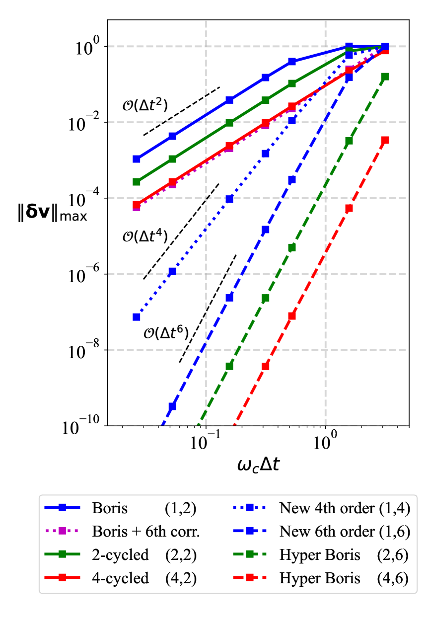
Figure 2: Scaling of maximum numerical errors in the velocity $\bm{v}$, as a function of the timestep $\omega_{c}\Delta t$. The label $(n,N)$ indicates $n$-cycled $N$th order solver.

5 Hyper Boris solver

Both the multicycle method (Section 3) and the higher-order correction (Section 4) use the standard 4-step procedure (Eq. (9)). The former repeats the 4-step procedure multiple times, and the latter corrects the electromagnetic vectors prior to the 4-step procedure. In other words, the two methods do not modify the 4-step procedure itself. Recognizing this fact, we propose a hybrid solver of the multicycle method and the higher-order correction to achieve even better accuracy. In practice, we corrects the electromagnetic vectors, before using the multicycle procedure. The entire procedure is as follows.

1. (Advance the particle position ${\bm{x}^{t+\Delta t/2}\leftarrow\bm{x}^{t-\Delta t/2}}+\bm{v}^{t}{\Delta t}$)

2. Define the element magnetic and electric vectors, $\bm{\tau}_{n}$ and $\bm{\varepsilon}_{n}$ (Eq. (22))

3. Referring to Eq. (11), set $f_{N}(\tau_{n})$ to a truncated Taylor expansion of $f(\tau_{n})$ up to $(N-2)$th order. Note that this is not $\tau_{1}$ but $\tau_{n}$.

4. Referring to Eqs. (12) and (58), calculate the magnetic and electric vectors $\bm{t}_{n}$ and $\bm{e}_{n}$

   $$\bm{t}_{n}\equiv f_{N}\,\bm{\tau_{n}},~~~\bm{e}_{n}\equiv f_{N}\,\bm{\varepsilon}_{n}+\Big{(}1-f_{N}\Big{)}\frac{(\bm{\varepsilon}_{n}\cdot\bm{\tau}_{n})\bm{\tau}_{n}}{\tau_{n}^{2}}$$ (60)

5. Calculate the four coefficients $c_{n1},c_{n2},c_{n3}$, and $c_{n6}$ (Eqs. (40)–(46))

6. Compute the next state $\bm{v}^{t+\Delta t}$ by the multicycle formula (Eq. (39))

We call this the hyper Boris solver, because it has two hyperparameters, $n$ and $N$. One can consider arbitrary combinations of the subcycling number $n$ and $N$th-order accuracy. Their combination excellently works, as will be shown in Section 6.

6 Numerical tests

In order to test the proposed solvers, we have carried out test-particle simulations in a static electromagnetic field. The following solvers are compared:

1. Boris solver with and without the 6th-order gyrophase correction [4]

2. Multicycle Boris solver ($n=2,4$), proposed in Section 3

3. New higher-order Boris solver ($N=4,6$) in Section 4

4. Hyper Boris solver $(n,N)=(2,6),(4,6)$ proposed in Section 5

The particle parameters are set to be $m=1$, $q=1$, $\bm{x}=(0,0,0)$, and $\bm{v}=(0,0,0)$. The electromagnetic fields are set to be $\bm{E}=(0,0.5,0.1)$ and $\bm{B}=(0,0,1)$. The gyro frequency is $\omega_{c}\equiv(qB/m)=1$. In each run, we evaluate an error in the velocity, $\|\bm{v}-\bm{v}_{\rm exact}\|$, where $\bm{v}_{\rm exact}$ is given by Eq. (4). Then we have recorded the maximum error during the six gyroperiods, $0<\omega_{c}t\leq 12\pi$. The timestep ranges from $\omega_{c}\Delta t=\pi/120$ to $\pi$.

Figure 2 shows the results as a function of the timestep $\Delta t$. The standard Boris solver is indicated by the blue solid line. It is evident that it provides the second-order error. Although partially hidden by the red solid line (the $n=4$ multicycle solver), the magenta dotted line indicates the Boris solver with the 6th-order gyrophase correction. It provides smaller errors than the standard Boris solver, but eventually returns the second-order error. The multicycle Boris solvers, indicated by the color solid lines, give expected results. They provide $n^{2}$ times smaller errors than the Boris solver. By definition, the Boris solver does not give a good approximation for $\omega_{c}\Delta t\gtrsim\pi/2$, but the multicycle solvers relax this threshold to $\omega_{c}\Delta t\gtrsim n\pi/2$. The blue dotted and dashed lines indicate the new higher-order Boris solvers. They have $N$th-order accuracy, $\propto(\Delta t)^{N}$, in contrast to the Boris solver with 6th-order gyrophase correction. Finally, the hyper Boris solvers are indicated by the color dashed lines. Since the two improvements work together, they give even better results. Now the error is proportional to $\propto(\Delta t/n)^{N}$.

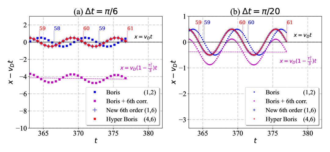
Figure 3: Particle positions in the E$\times$B drift frame $(x-v_{D}t)$ as a function of time $t$, for (a) $\omega_{c}\Delta t=\pi/6$ and (b) $\omega_{c}\Delta t=\pi/20$. The drift speed is set to be $v_{D}=\|\bm{E}\times\bm{B}\|/B^{2}=0.5$. Four particle solvers are compared. The solid red curve indicates the analytic solution. The magenta dashed line indicates the erroneous drift effect of $\approx v_{D}(1-\tau_{1}^{2}/3)t$ (Eq. (61)). The red and blue numbers such as ‘60’ indicate the starting points of the 60th gyroperiod.

Next, in order to check long-term behaviors, we run test particle simulations in the same electromagnetic field over sixty gyroperiods, $\omega_{c}t\leq 120\pi$. Panels in Fig. 3 show particle positions as a function of time for (a) $\omega_{c}\Delta t=\pi/6\approx 0.52$ and (b) $\omega_{c}\Delta t=\pi/20\approx 0.16$. In these cases, while gyrating, the particles drift in the $+x$ direction. Then the $x$-positions in the E$\times$B drift frame are presented, i.e., $(x-v_{D}t)$, where $v_{D}=\|\bm{E}\times\bm{B}\|/B^{2}=0.5$ is the drift speed. The symbols indicate the results of the four particle solvers. The red solid line indicates the analytic solution of particle position. One can see that the gyrophase in the standard Boris solver (the blue squares) differs from the others, because of a numerical delay in phase. There is a larger delay in the $\omega_{c}\Delta t=\pi/6$ case, because of the second-order error in gyrophase. In contrast, even though it better reproduces the gyrophase, the Boris solver with the 6th-order gyrophase correction (the purple squares) moves in $+x$ at the erroneously slow speed. This is in agreement with our estimate (Eq. (57)),

$$\frac{1}{f_{6}}\frac{\|\bm{E}\times\bm{B}\|}{B^{2}}=v_{D}\left(1-\frac{1}{3}\tau_{1}^{2}+\mathcal{O}(\tau_{1}^{4})\right)$$ (61)

The new 6th-order Boris solver and the $(4,6)$ hyper Boris solver do not exhibit this drift-speed problem. Their results are virtually indistinguishable from the exact solutions in Figs. 3(a) and (b). Strictly speaking, there remain small displacements between the particle positions and the exact positions, $\|\bm{r}-\bm{r}_{\rm exact}\|=0.006\sim 0.017\ll r_{L}$, where $r_{L}=|\bm{v}_{\rm t=0}-\bm{v}_{D}|/\omega_{c}=0.5$ is the typical gyroradius, because we advance the particle by the leap-frog method. This second-order displacement does not grow in time.

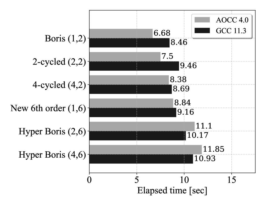
Figure 4: Elapsed time of test-particle simulations by the Boris solver and the hyper Boris solvers. The label $(n,N)$ indicates $n$-cycled $N$th order solver.

In order to evaluate the computational cost, we run the same simulations with $\omega_{c}\Delta t=\pi/6$ until $\omega_{c}t=10^{8}\pi$ on our Linux PC with AMD Ryzen 5955WX processor. We use the AMD optimizing fortran compiler (AOCC) 4.0 and GNU Compiler Collection (GCC) 11.3 with the -O2 option. We use the standard 4-step procedure (Eq. (9)) for $n=1$ and the multicycle formula (Eq. (39)) for $n=2,4$. Their elapsed times are compared in Fig. 4. Thanks to the formula, the program does not need to repeat the 4-step procedure, and therefore the numerical cost increases only reasonably. The field correction requires additional cost. The 4-cycled 6th-order solver is 30–75% more expensive than the standard Boris solver. Even though the benchmark results highly depend on the specific implementation, compiler, and computer, these results suggest that the proposed solvers are promising. For comparison, we have also implemented and tested a direct solver, which uses Eq. (4) in the simulation. In this case, as mentioned earlier, we need to deal with the division by zero inside the sinc function and in the last term, because $\tau_{1}$ can be zero. We only found that the direct solver is substantially slower than other integrators: it took 25.63 (AOCC) and 19.91 (GCC) seconds in the same test. This confirms that the approximate integrators are useful.

7 Discussion

In this article, we have discussed three improvements to the Boris integrator for kinetic plasma simulations. First, we have proposed the multicycle method. Partial or full sub-stepping of the particle integrator was proposed by many authors [1, 6, 2, 16, 17, 22]; however, our unique point is that we have derived and utilized the multicycle formula (Eq. (39)) for arbitrary $n$ for the acceleration part of the particle integrator. The formula contains six coefficients. Conveniently, we only need to calculate four coefficients, because among the six coefficients there are two pairs of coefficients each of which are identical. Second, prior to the 4-step procedure, we use the gyrophase correction to $\bm{B}$ and the anisotropic correction to $\bm{E}$ to achieve higher-order accuracy. A similar idea was discussed in earlier literature (Section 4.3 (p.60) in Birdsall & Langdon [3]; Section 4.7.1 (p.114) in Hockney & Eastwood [8]), but it has not been used over many decades. Third, combining the subcycling and the higher-order correction, we have proposed the hyper Boris solver. We summarize all the procedures in Section 5. It only gives a numerical error of $\propto(\Delta t/n)^{N}$, as confirmed by numerical tests in Section 6.

It is noteworthy that all the solvers are reversible. As evident in Eq. (32), the multicycle procedures are symmetric in time. The higher-order correction is time-symmetric as well, because it uses the electromagnetic fields at the time center $t+\Delta t/2$. So is the hyper Boris solver, because it is a hybrid of the two. We expect that such a time-symmetric solver is stable, because the particle motion is unlikely to be damped or amplified in one specific direction. Another favorable property for the long-term stability is the incompressibility in the phase-space volume, often denoted as the volume-preservation [14]. Eq. (54) and subsequent discussion tell us that the Boris solver with higher-order correction gives a rotation by the angle of $2\alpha_{1,corr}$ and a parallel displacement by $({q\bm{E}_{\parallel}}/m)\Delta t$ in the velocity space. These operations conserve a volume in the velocity-space, and the hyper Boris solver inherits this property. Together with the position part, the hyper Boris solver is volume preserving, similar to the original Boris solver.

The hyper Boris solvers give accurate results at affordable costs. Our numerical tests show that the 4-cycle 6th-order solver needs 30–75% more computational time than the standard Boris solver. Considering its ultrahigh accuracy, this is acceptable. It is also noteworthy that we can reduce the total computational cost, by employing a higher-accuracy solver and a larger timestep $\Delta t$. Our recommendation is $(n,N)=(2,6)$ or $(4,6)$. This is because the 4th-order and 6th-order corrections are not so much different in complexity, and because multi cycles ($n\geq 2$) significantly improve the accuracy for large $\omega_{c}\Delta t$.

Owing to higher accuracy, the hyper Boris solver allows us to use a larger timestep in kinetic simulations. In practice, many factors would limit the timestep. To preserve an apparent gyroradius $r_{L}\approx|\bm{v}-\bm{v}_{D}|/\omega_{c}$, one may want to keep $\omega_{c}\Delta t\lesssim 0.5$–$1.0$, as discussed in Ref. [22]. In PIC simulation, it would be necessary to keep $\Delta t$ small, so that the particle either stays in the same cell or moves to the adjacent cells. Also, the plasma frequency $\omega_{p}$ often constrains $\Delta t$ [3, 20]. Similar to the standard Boris solver, the hyper Boris solver uses the electric and magnetic field at the particle position, which is interpolated from the field in the grid cells. To take full advantage of the higher accuracy in time, it would be useful to interpolate the electromagnetic field at higher-order accuracy with respect to the grid size $\Delta x$. For example, we may need a longer stencil in space [10]. This also involves many other issues such as the self-force and the charge-conservation in PIC simulation. Coupling of the temporal and spatial accuracy needs further investigation.

The hyper Boris solver is nonrelativistic. It cannot be applied to the relativistic particle motion, because the Lorentz factor makes the problem difficult. The subcycling should be useful in the relativistic regime; however, we can no longer use the formula (Eq. (39)), because the Lorentz factor changes every subcycle. We have also used the nonrelativistic formula (Eq. (55)) to derive the higher-order correction. It is not clear whether there is a simple form of a relativistic correction. This is left for future research. For a moment, we recommend the users other Boris-type solvers [16, 21, 22] that improve the Lorentz-force part of the relativistic Newton–Lorentz equation.

Finally, in addition to the Newton–Lorentz equation, the hyper Boris solver can be applied to the particle motion in a differentially rotating system [15, 9], because the equation of motion can be transformed into the Newton–Lorentz equation [9, Appendix C]. Similarly, we expect that the hyper Boris solver is useful for differential equations in the form of $(d/dt)\bm{v}=\bm{A}+\bm{v}\times\bm{B}$.

Author Contributions

SZ: Conceptualization (lead); Formal analysis (equal); Funding acquisition (lead); Investigation (lead); Methodology (equal); Visualization; Writing – original draft; Writing – review & editing (equal). TK: Formal analysis (equal); Methodology (equal); Writing – review & editing (equal).

Conflict of Interest

The authors have no conflicts to disclose.

Data availability

The data will be available from the corresponding author upon reasonable request.

Appendix A Derivation of Eq. (4)

In constant electromagnetic fields, the equation of motion

$$\frac{d\bm{v}}{dt} =\frac{q}{m}\left(\bm{E}+{\bm{v}}\times\bm{B}\right)$$ (62)

gives a gyration around the E$\times$B velocity:

$$\left(\bm{v}^{t+\Delta t}-\frac{\bm{E}\times\bm{B}}{B^{2}}\right) =\left(\bm{v}^{t}-\frac{\bm{E}\times\bm{B}}{B^{2}}\right)\cos\theta+\bigg{(}\Big{(}\bm{v}^{t}-\frac{\bm{E}\times\bm{B}}{B^{2}}\Big{)}\times\bm{\hat{b}}\bigg{)}\sin\theta$$

$$~~~~+\left(\bm{v}^{t}-\frac{\bm{E}\times\bm{B}}{B^{2}}\right)_{\parallel}(1-\cos\theta)+\frac{q\bm{E}_{\parallel}}{m}\Delta t.$$ (63)

where $\theta$ is given by Eq. (10). We rewrite this by using $\bm{\tau}_{1}$ and $\bm{\varepsilon}_{1}$:

$$\left(\bm{v}^{t+\Delta t}-\frac{\bm{\varepsilon}_{1}\times\bm{\tau}_{1}}{{\tau}_{1}^{2}}\right) =\left(\bm{v}^{t}-\frac{\bm{\varepsilon}_{1}\times\bm{\tau}_{1}}{{\tau}_{1}^{2}}\right)\cos 2\tau_{1}+\bigg{(}\Big{(}\bm{v}^{t}-\frac{\bm{\varepsilon}_{1}\times\bm{\tau}_{1}}{{\tau}_{1}^{2}}\Big{)}\times\frac{\bm{\tau}_{1}}{\tau_{1}}\bigg{)}\sin 2\tau_{1}$$

$$~~~~+(1-\cos 2\tau_{1})\left(\left(\bm{v}^{t}-\frac{\bm{\varepsilon}_{1}\times\bm{\tau}_{1}}{{\tau}_{1}^{2}}\right)\cdot\frac{\bm{\tau}_{1}}{\tau_{1}}\right)\frac{\bm{\tau}_{1}}{\tau_{1}}+2\left(\bm{\varepsilon}_{1}\cdot\frac{\bm{\tau}_{1}}{\tau_{1}}\right)\frac{\bm{\tau}_{1}}{\tau_{1}}$$ (64)

This leads to the following solution.

$$\bm{v}^{t+\Delta t} =\cos 2\tau_{1}\bm{v}^{t}+\frac{2\sin 2\tau_{1}}{2\tau_{1}}\bigg{(}\bm{v}^{t}\times{\bm{\tau}_{1}}+\bm{\varepsilon}_{1}\bigg{)}$$

$$~~~~+\frac{(1-\cos 2\tau_{1})}{\tau_{1}^{2}}\Big{(}\left(\bm{v}^{t}\cdot\bm{\tau}_{1}\right)\bm{\tau}_{1}+\bm{\varepsilon}_{1}\times\bm{\tau}_{1}\Big{)}+\frac{2}{\tau_{1}^{2}}\bigg{(}1-\frac{\sin 2\tau_{1}}{2\tau_{1}}\bigg{)}{\left(\bm{\varepsilon}_{1}\cdot\bm{\tau}_{1}\right)\bm{\tau}_{1}}$$ (65)

One can further rewrite this, by using the sinc function: ${\rm sinc}(x)\equiv\sin(x)/x$.

$$\bm{v}^{t+\Delta t} =\cos(2\tau_{1})\bm{v}^{t}+2{\rm sinc}(2\tau_{1})(\bm{v}^{t}\times\bm{\tau}_{1}+\bm{\varepsilon}_{1})$$

$$~~~+2{\rm sinc}^{2}(\tau_{1})\Big{(}(\bm{v}^{t}\cdot\bm{\tau}_{1})\bm{\tau}_{1}+\bm{\varepsilon}_{1}\times\bm{\tau}_{1}\Big{)}+\frac{2(1-{\rm sinc}(2\tau_{1}))}{\tau_{1}^{2}}(\bm{\varepsilon}\cdot\bm{\tau}_{1})\bm{\tau}_{1},$$ (66)

References

- Adam et al. [1982] J. C. Adam, A. G. Serveniere, A. B. Langdon, J. Comput. Phys. 47 (1982) 229.
- Arefiev et al. [2015] A. V. Arefiev, G. E. Cochran, D. W. Schumacher, A. P. L. Robinson, G. Chen, Phys. Plasmas 22 (2015) 013103.
- Birdsall & Langdon [1985] C. K. Birdsall, A. B. Langdon, Plasma Physics via Computer Simulation, McGraw-Hill, New York, 1985.
- Boris [1970] J. P. Boris, in Proceedings of 4th Conference on Numerical Simulation of Plasmas, Naval Research Laboratory, Washington D. C., 1970, pp. 3–67.
- Buneman [1967] O. Buneman, J. Comput. Phys. 1 (1967) 517.
- Friedman et al. [1991] A. Friedman, S. E. Parker, S. Ray, C. K. Birdsall, J. Comput. Phys. 96 (1991) 54.
- He et al. [2015] Y. He, Y. Sun, J. Liu, H. Qin, J. Comput. Phys. 281 (2015) 135.
- Hockney & Eastwood [1981] R. W. Hockney & J. W. Eastwood, Computer simulation using particles, McGraw-Hill, New York, 1981.
- Hoshino [2013] M. Hoshino, Astrophys. J. 773 (2013) 118.
- Lehe et al. [2014] R. Lehe, C. Thaury, E. Guillaume, A. Lifschitz, V. Malka, Phys. Rev. ST Accel. Beams 17 (2014) 121301.
- Lipatov [2002] A. S. Lipatov, The Hybrid Multiscale Simulation Technology, Springer, Berlin, 2002.
- Kato & Zenitani [2021] T.-N. Kato, S. Zenitani, arXiv preprint (2021) arxiv:2108.02426.
- Patacchini & Hutchinson [2009] L. Patacchini, I. H. Hutchinson, J. Comput. Phys. 228 (2009) 2604.
- Qin et al. [2013] H. Qin, S. Zhang, J. Xiao, J. Liu, Y. Sun, W. M. Tang, Phys. Plasmas 20 (2013) 084503.
- Riquelme et al. [2012] M. A. Riquelme, E. Quataert, P. Sharma, A. Spitkovsky, Astrophys. J. 755 (2012) 50
- Umeda [2018] T. Umeda, Comput. Phys. Commun. 228 (2018) 1.
- Umeda [2019] T. Umeda, Comput. Phys. Commun. 237 (2019) 37.
- Verboncoeur [2005] J. P. Verboncoeur, Plasma Phys. Control. Fusion 47 (2005) A231.
- Winkel et al. [2015] M. Winkel, R. Speck, D. Ruprecht, J. Comput. Phys. 295 (2015) 456.
- Winske & Omidi [1996] D. Winske, N. Omidi, J. Geophys. Res. 101 (1996) 17287.
- Zenitani & Umeda [2018] S. Zenitani, T. Umeda, Phys. Plasmas 25 (2018) 112110.
- Zenitani & Kato [2020] S. Zenitani, T.-N. Kato, Comput. Phys. Commun. 247 (2020) 106954.