Stochastic dominance for linear combinations of infinite-mean risks

Abstract

In this paper, we establish a sufficient condition to compare linear combinations of independent and identically distributed (iid) infinite-mean random variables under usual stochastic order. We introduce a new class of distributions that includes many commonly used heavy-tailed distributions and show that within this class, a linear combination of random variables is stochastically larger when its weight vector is smaller in the sense of majorization order. We proceed to study the case where each random variable is a compound Poisson sum and demonstrate that if the stochastic dominance relation holds, the summand of the compound Poisson sum belongs to our new class of distributions. Additional discussions are presented for stable distributions.

Keywords: infinite mean; heavy-tailed distributions; usual stochastic order; majorization order.

MSC2020: 60E05; 60E15.

1 Introduction

Linear combinations of random variables play a crucial role in various fields, including statistics, operations research, reliability theory, and actuarial science. Over the past few decades, extensive studies and advances have been made in comparing linear combinations of random variables. For example, see Proschan (1965), Ma (1998, 2000), Ibragimov, (2005, 2009), Xu and Hu (2011), Yu (2011), Zhao et al. (2011), Pan et al. (2013), Mao et al. (2013), and Zhang and Cheung (2020).

Let $X_{1},\dots,X_{n}$ be independent and identically distributed (iid) random variables. Given two non-negative real vectors $(\theta_{1},\dots,\theta_{n})$ and $(\eta_{1},\dots,\eta_{n})$ such that $(\theta_{1},\dots,\theta_{n})$ is smaller than $(\eta_{1},\dots,\eta_{n})$ in majorization order (see Definition 1), a typical problem in this area is to compare $\sum_{i=1}^{n}\theta_{i}X_{i}$ and $\sum_{i=1}^{n}\eta_{i}X_{i}$ via some notion of stochastic dominance. In the seminal work of Proschan (1965), it is shown that for iid symmetric log-concavely distributed $X_{1},\dots,X_{n}$, $\sum_{i=1}^{n}\theta_{i}X_{i}$ is more peaked than $\sum_{i=1}^{n}\eta_{i}X_{i}$, i.e., $\mathbb{P}(|\sum_{i=1}^{n}\theta_{i}X_{i}|\leq x)\geq\mathbb{P}(|\sum_{i=1}^{n}\eta_{i}X_{i}|\leq x)$ for all $x>0$. This remarkable result was subsequently extended and found applications in economics, statistics, and operations research; see, e.g., Ibragimov, (2005) and the references therein. Notably, Ibragimov, (2005) showed that the peakedness property for log-concave distributions continues to hold for stable distributions with finite mean. A closely related result is that for all iid finite-mean random variables, $\sum_{i=1}^{n}\theta_{i}X_{i}$ is smaller than $\sum_{i=1}^{n}\eta_{i}X_{i}$ in convex order (see, e.g., Theorem 3.A.35 of Shaked and Shanthikumar (2007) and Property 3.4.48 of Denuit et al. (2005)). The above peakedness property and the relation in convex order both suggest that $\sum_{i=1}^{n}\theta_{i}X_{i}$ is less spread-out than $\sum_{i=1}^{n}\eta_{i}X_{i}$.

A key assumption for the above results to hold is that random variables have a finite mean. If the mean of random variables is infinite, the observations for finite-mean models can be quite different or even flipped; see Chen and Wang (2025) for a survey on infinite-mean models in the realms of finance and insurance. For instance, if $X_{1},\dots,X_{n}$ are iid stable random variables with tail parameter strictly less than 1 (thus infinite mean), Ibragimov, (2005) showed that $\sum_{i=1}^{n}\theta_{i}X_{i}$ is less peaked than $\sum_{i=1}^{n}\eta_{i}X_{i}$. In particular, for such stable random variables that are always positive, this result can be equivalently written as

$$\sum_{i=1}^{n}\eta_{i}X_{i}\leq_{\rm st}\sum_{i=1}^{n}\theta_{i}X_{i},$$ (1)

where $\leq_{\rm st}$ denotes usual stochastic order. For two random variables $X$ and $Y$, $X$ is said to be smaller than $Y$ in usual stochastic order if $\mathbb{P}(X\leq x)\geq\mathbb{P}(Y\leq x)$ for all $x\in\mathbb{R}$; for properties of stochastic orders, we refer to Müller and Stoyan, (2002) and Shaked and Shanthikumar (2007). Chen et al., (2025) have recently shown that (1) also holds for Pareto distributions with infinite mean; a special case of (1) for two Pareto random variables with tail parameter 1/2 was previously studied by Embrechts et al., (2002).

Inequality (1) provides an intuitive implication in portfolio diversification: A more diversified portfolio is stochastically larger; see Ibragimov, (2009), Ibragimov et al. (2011), and Nešlehová et al., (2006) for the diversification effects of infinite-mean models in different contexts. Another application of (1) can be found in the optimal bundling problems of Ibragimov and Walden, (2010).

Given its potential applicability, this paper aims to explore sufficient and necessary conditions for (1) to hold. In Section 2, we introduce a new class of distributions, denoted by $\mathcal{H}$, and show that (1) holds for all distributions in $\mathcal{H}$ (Theorem 1). Using the established majorization theory, we present a simple characterization of the continuous distributions in $\mathcal{H}$ (see Propositions 2 (ii)). We apply this characterization to show that many commonly used heavy-tailed distributions belong to $\mathcal{H}$. Together with some closure properties of $\mathcal{H}$ (Propositions 3-5), we demonstrate that the new class is rather rich. We note here that the techniques used in Ibragimov, (2005) and Chen et al., (2025) are designed specifically for stable distributions and Pareto distributions respectively, and there does not seem to be a way to generalize them to other distributions. We develop and apply different methods to prove our main result in Theorem 1.

In Sections 3 and 4, we proceed to study (1) for different classes of distributions. Section 3 assumes that each of $X_{1},\dots,X_{n}$ follows a compound Poisson distribution, which is a standard model for portfolio claims and aggregate risks in banking and insurance sectors; see, e.g., Kaas et al., (2008). Assuming that each summand of the compound Poisson sum is a non-negative random variable, Theorem 3 shows that (1) holds if and only if the distribution of each summand belongs to class $\mathcal{H}$. Section 4 presents further discussions of (1) for stable distributions, complementing the findings of Ibragimov, (2005), who focused on the peakedness property of linear combinations of stable random variables. Section 5 concludes the paper with some open questions. The appendices provide more details for Table 1, which contains further examples of distributions from $\mathcal{H}$, as well as details of the simulation procedure for stable distributions used in the numerical illustration.

Notation

We fix some notation here. Denote by $\mathbb{N}$ the set of all positive integers, $\mathbb{R}_{+}$ the set of all non-negative real numbers, and $\mathbb{R}_{++}$ the set of all positive real numbers. Let $\mathbb{N}_{0}=\mathbb{N}\cup\{0\}$. For $n\in\mathbb{N}$, let $[n]=\{1,\dots,n\}$. Throughout, $n$ is assumed to be larger than or equal to 2. We use $\overline{\theta}$ and $\overline{\eta}$ to denote vectors $(\theta_{1},\dots,\theta_{n})\in\mathbb{R}_{+}^{n}$ and $(\eta_{1},\dots,\eta_{n})\in\mathbb{R}_{+}^{n}$, respectively. Denote by $\varphi_{X}$ the characteristic function of a random variable $X$. For a distribution $F$, define its tail function $\overline{F}=1-F$ and essential infimum $\operatorname*{ess\text{-}inf}F$. We use $\simeq_{\rm st}$ for equality in distribution.

2 Stochastic dominance and a class of distributions

2.1 A stochastic dominance relation

We first recall the notion of majorization order.

Definition 1.

For two vectors $\overline{\theta}:=\left(\theta_{1},\dots,\theta_{n}\right)$ and $\overline{\eta}:=\left(\eta_{1},\dots,\eta_{n}\right)$ in $\mathbb{R}^{n}$, $\overline{\theta}$ is dominated by $\overline{\eta}$ in majorization order, denoted by $\overline{\theta}\preceq\overline{\eta}$ if

$$\sum^{n}_{i=1}\theta_{i}=\sum^{n}_{i=1}\eta_{i}\mbox{~~~and~~~}\sum^{k}_{i=1}\theta_{(i)}\geq\sum^{k}_{i=1}\eta_{(i)}\ \ \mbox{for}\ k\in[n-1],$$

where $\theta_{(i)}$ and $\eta_{(i)}$ represent the $i$th smallest order statistics of $\overline{\theta}$ and $\overline{\eta}$, respectively.

The main focus of the paper is on studying the following stochastic dominance relation

$$\sum_{i=1}^{n}\eta_{i}X_{i}\leq_{\rm st}\sum_{i=1}^{n}\theta_{i}X_{i}\mbox{ for all $\overline{\theta},\overline{\eta}\in\mathbb{R}^{n}_{+}$ such that $\overline{\theta}\preceq\overline{\eta}$,}$$ (SD)

where $X_{1},\dots,X_{n}$ are iid random variables. Let $X$ be a copy of $X_{1},\dots,X_{n}$. If $X_{1},\dots,X_{n}\sim F$ satisfy (SD), we also say $X$ or $F$ satisfies (SD). For some $x\in\mathbb{R}$, let

$$g(\theta_{1},\dots,\theta_{n})=\mathbb{P}\left(\sum_{i=1}^{n}\theta_{i}X_{i}>x\right),~~\overline{\theta}\in\mathbb{R}^{n}_{+}.$$

Then (SD) holds if and only if $g$ is Schur-concave on $\mathbb{R}^{n}_{+}$ for all $x\in\mathbb{R}$; recall that a function $f$ on $\mathbb{R}^{n}$ is Schur-concave if $f(\overline{x})\geq f(\overline{y})$ for $\overline{x}\preceq\overline{y}$.

We present below some elementary properties of (SD).

Proposition 1.

The following statements hold.

1. If random variable $X$ satisfies (SD), then either $X$ is a constant, or $\mathbb{E}[|X|]$ is infinite.

2. If two independent random variables $X$ and $Y$ satisfy (SD), then $X+Y$ satisfies (SD).

3. If random variable $X$ satisfies (SD), then $(X+a)/b$ satisfies (SD) for all $a\in\mathbb{R}$ and $b\in\mathbb{R}_{++}$.

4. If $Y_{k}$ with $k=1,2,\dots$ satisfies (SD) and $Y_{k}\xrightarrow{\mathrm{d}}X$, then $X$ satisfies (SD).

Proof.

If $X$ is a constant, (SD) clearly holds. For a non-degenerate random variable $X$, as (SD) implies $(\sum_{i=1}^{n}\theta_{i})X\leq_{\rm st}\sum_{i=1}^{n}\theta_{i}X_{i}$, by Theorem 2.3 (b) of Müller, (2024), $\mathbb{E}[|X|]=\infty$. Statement (ii) is because usual stochastic order is preserved under convolution (see, e.g., Theorem 1.A.3 (b) of Shaked and Shanthikumar (2007)). Statement (iii) is trivial. Statement (iv) holds as usual stochastic order is preserved under convergence in distribution (Theorem 1.2.14 of Müller and Stoyan, (2002)). ∎

Remark 1.

Property (SD) implies that $(X_{1}+\dots+X_{n})/n$ is increasing in usual stochastic order as $n$ increases, since $(1/n,\dots,1/n,0)$ dominates $(1/(n+1),\dots,1/(n+1))$ in majorization order for all $n$. By Proposition 1, if $X_{1}$ satisfies (SD) and $X_{1}$ is bounded from below, we have $\mathbb{E}[X_{1}]=\infty$. Then by the law of large numbers, $(X_{1}+\dots+X_{n})/n\rightarrow\infty$ almost surely as $n$ goes to infinity (see, e.g., Theorem 2.4.5 of Durrett, (2019)).

2.2 A new class of distributions

Next, we introduce a class of distributions of non-negative random variables, denoted by $\mathcal{H}$. We will show later that this rather large class of distributions satisfies property (SD) and thus, by Proposition 1, the distributions in $\mathcal{H}$ have infinite mean.

Definition 2.

Let $F$ be a distribution function with $\operatorname*{ess\text{-}inf}F=0$. We say $F\in\mathcal{H}$ if the function

$$\phi(x_{1},x_{2})=\overline{F}\left(\frac{1}{x_{1}}\right)+\overline{F}\left(\frac{1}{x_{2}}\right),~~(x_{1},x_{2})\in\mathbb{R}_{++}^{2}$$

is Schur-concave. For $X\sim F$ where $F\in\mathcal{H}$, we also write $X\in\mathcal{H}$.

The following result characterizes distributions in class $\mathcal{H}$.

Proposition 2.

The following statements hold.

1. A distribution function $F\in\mathcal{H}$ if and only if $\overline{F}(1/x)=c(x)+a(x)$ where $c:\mathbb{R}_{++}\rightarrow\mathbb{R}$ is concave and $a:\mathbb{R}_{++}\rightarrow\mathbb{R}$ is additive.

2. Let $F$ be a continuous distribution on $\mathbb{R}_{+}$. Then $F\in\mathcal{H}$ if and only if $\overline{F}(1/x)$ is concave in $x\in\mathbb{R}_{++}$. In addition, if $F$ has density $f$, then $F\in\mathcal{H}$ if and only if $x^{2}f(x)$ is increasing in $x\in\mathbb{R}_{++}$.

Proof.

1. This follows from Theorem 3 of Ng, (1987).

2. By 3.C.1 of Marshall et al. (2011), if $g:\mathbb{R}_{+}\rightarrow\mathbb{R}_{+}$ is concave, then $\phi(x_{1},\dots,x_{n})=\sum_{i=1}^{n}g(x_{i})$ is Schur-concave in $(x_{1},\dots,x_{n})\in\mathbb{R}_{+}^{n}$. Thus, we have the “$\Leftarrow$” direction. By 3.C.1.c of Marshall et al. (2011), for a continuous function $g$ on an interval $I$, if $\psi(x_{1},x_{2})=g(x_{1})+g(x_{2})$ is Schur-concave on $I^{2}$, then $g$ is concave. Then the “$\Rightarrow$” direction follows. ∎

Remark 2.

If distributions have densities of the form $f(x)=x^{-\alpha-1}l(x)$ where function $l$ is increasing and $\alpha\in(0,1]$, the distributions are in $\mathcal{H}$ by Proposition 2. In addition, if $l$ is a slowly-varying function, by the Karamata representation (see Theorem B.1.6 of de Haan and Ferreira (2006)), it may be written as

$$l(x)=\exp\left(c(x)+\int_{0}^{x}\frac{\varepsilon(t)}{t}\mathrm{d}t\right),$$

where $c(x)\to c$ as $x\to\infty$ and $\varepsilon(x)\to 0$ as $x\to\infty$. If $c$ is increasing and $\varepsilon$ is non-negative, the distributions are in $\mathcal{H}$.

One can use Proposition 2 (ii) together with Remark 2 to show that many commonly used heavy-tailed distributions are in $\mathcal{H}$. We present some examples below. Additional examples are collected in Table 1; see Appendix A for more details of Table 1. Some closure properties of $\mathcal{H}$ are collected in Section 2.4.

Example 1 (Fréchet distribution).

The Fréchet distribution function is $F(x)=\exp\left(-x^{-\alpha}\right)$, $x\in\mathbb{R}_{++}$. As its density function is $f(x)=\alpha x^{-\alpha-1}\exp\left(-x^{-\alpha}\right)$ for $x\in\mathbb{R}_{++}$, by Remark 2, $F\in\mathcal{H}$ if $\alpha\leq 1$.

Example 2 (Absolute Cauchy distribution).

The absolute Cauchy distribution is defined as $F(x)=(2/\pi)\arctan(x)$ for $x\in\mathbb{R}_{++}$. As the density function is $f(x)=2/(\pi(x^{2}+1))=x^{-2}(2x^{2}/(\pi(x^{2}+1)))$ for $x\in\mathbb{R}_{++}$, by Remark 2, we have $F\in\mathcal{H}$.

Example 3 (Inverse Gamma distribution).

The density function of the inverse Gamma distribution with parameters $\alpha,\beta\in\mathbb{R}_{++}$ is $f(x)=\beta^{\alpha}x^{-\alpha-1}\exp\left(-\beta/x\right)/\Gamma(\alpha)$, $x\in\mathbb{R}_{++}$. By Remark 2, if $\alpha\leq 1$ and $\beta\in\mathbb{R}_{++}$, we have $F\in\mathcal{H}$. The inverse Gamma distribution with $\alpha=0.5$ is the Lévy distribution, which also belongs to the class of stable distributions.

Example 4 (Feller-Pareto distribution).

The Feller-Pareto distribution with parameters $\mu\in\mathbb{R}$ and $\sigma,\gamma,\gamma_{1},\gamma_{2}\in\mathbb{R}_{++}$, denoted by ${\rm FP}(\mu,\sigma,\gamma,\gamma_{1},\gamma_{2})$, has the density function

$$f(x)=\frac{1}{\gamma\sigma B(\gamma_{1},\gamma_{2})}\left(\frac{x-\mu}{\sigma}\right)^{(\gamma_{2}/\gamma)-1}\left(1+\left(\frac{x-\mu}{\sigma}\right)^{1/\gamma}\right)^{-\gamma_{1}-\gamma_{2}},~~x>\mu,$$

where $B$ is the beta function. The class of Feller-Pareto distributions is very general. If $\gamma_{2}=1$, the Feller-Pareto distribution becomes the Pareto type-IV distribution (${\rm FP}(\mu,\sigma,\gamma,\alpha,1)$), which includes the Pareto type-III distribution (${\rm FP}(\mu,\sigma,\gamma,1,1)$), the Pareto type-II distribution (${\rm FP}(\mu,\sigma,1,\alpha,1)$), and the Pareto type-I distribution (${\rm FP}(\sigma,\sigma,1,\alpha,1)$). Note that the Pareto type-IV distribution is essentially the Burr distribution. See Arnold, (2015) for the statistical properties of the Feller-Pareto distribution. Assume that $\mu=0$ and $\sigma=1$ and let $h(x)=x^{2}f(x)$ for $x\in\mathbb{R}_{+}$. Taking derivative of $h$, we have

$$h^{\prime}(x)=\frac{x^{\gamma_{2}/\gamma}\left(\left(x^{1/\gamma}+1\right)^{-\gamma_{1}-\gamma_{2}-1}\left((\gamma-\gamma_{1})x^{1/\gamma}+\gamma_{2}+\gamma\right)\right)}{\gamma^{2}B(\gamma_{1},\gamma_{2})}.$$

If $\gamma\geq\gamma_{1}$, i.e., the Feller-Pareto distribution has infinite mean, $h$ is increasing. By Proposition 2 (ii), the Feller-Pareto distribution is in $\mathcal{H}$ if $\gamma\geq\gamma_{1}$.

Table 1: Further examples of distributions in $\mathcal{H}$.

	Distribution functions	Parameters
Pareto distribution	$F(x)=1-(x+1)^{-\alpha},~~x\in\mathbb{R}_{++}$	$\alpha\leq 1$
Log-Pareto distribution	$F(x)=1-(\log(x+1)+1)^{-\alpha},~~x\in\mathbb{R}_{++}$	$\alpha\leq 2$
Inverse Burr distribution	$F(x)=(x^{\tau}/(x^{\tau}+1))^{\alpha},~~x\in\mathbb{R}_{++}$	$\tau\leq 1$, $\alpha>0$
Stoppa distribution	$F(x)=(1-(x+1)^{-\alpha})^{\beta},~~x\in\mathbb{R}_{++}$	$\alpha\leq 1$, $\beta\geq 1$
Log-Cauchy distribution	$F(x)=\arctan(\log(x))/\pi+1/2,~~x\in\mathbb{R}_{++}$	NA

2.3 Main result

Let $\overline{\theta}$ and $\overline{\eta}$ be two vectors in $\mathbb{R}^{n}$. Then $\overline{\theta}$ is a $T$-transform of $\overline{\eta}$ if for some $\lambda\in[0,1]$ and $i,j\in[n]$ with $i\neq j$,

$$\theta_{i}=\lambda\eta_{i}+(1-\lambda)\eta_{j},~\theta_{j}=(1-\lambda)\eta_{i}+\lambda\eta_{j},$$

and $\theta_{k}=\eta_{k}$ for $k\in[n]\setminus\{i,j\}$. The following lemma will be useful in our proof.

Lemma 1.

(Marshall et al., 2011, Section 1.A.3)  For $\overline{\theta},\overline{\eta}\in\mathbb{R}^{n}$, $\overline{\theta}\preceq\overline{\eta}$ if and only if $\overline{\theta}$ can be obtained from $\overline{\eta}$ by a finite number of $T$-transforms.

Theorem 1.

If $F\in\mathcal{H}$, then $F$ satisfies (SD).

Proof.

We first show that it is sufficient to prove the theorem for the case of two random variables. By Lemma 1, it suffices to assume that $\overline{\theta}$ is obtained from $\overline{\eta}$ by a $T$-transform, i.e., only two components in $\overline{\theta}$ and $\overline{\eta}$ are different. Write $\overline{\theta}=(\lambda\eta_{1}+(1-\lambda)\eta_{2},(1-\lambda)\eta_{1}+\lambda\eta_{2},\eta_{3},\dots,\eta_{n})$ for some $\lambda\in[0,1]$. If the statement of the theorem is correct for two random variables, then

$$\theta_{1}X_{1}+\theta_{2}X_{2}=(\lambda\eta_{1}+(1-\lambda)\eta_{2})X_{1}+((1-\lambda)\eta_{1}+\lambda\eta_{2})X_{2}\geq_{\rm st}\eta_{1}X_{1}+\eta_{2}X_{2}.$$

Then, as $X_{1},\dots,X_{n}$ are independent and usual stochastic order is closed under convolution (see, e.g., Theorem 1.A.3 (b) of Shaked and Shanthikumar (2007)),

$$\sum_{i=1}^{n}\theta_{i}X_{i} =(\lambda\eta_{1}+(1-\lambda)\eta_{2})X_{1}+((1-\lambda)\eta_{1}+\lambda\eta_{2})X_{2}+\sum_{i=3}^{n}\eta_{i}X_{i}$$

$$\geq_{\rm st}\eta_{1}X_{1}+\eta_{2}X_{2}+\sum_{i=3}^{n}\eta_{i}X_{i}=\sum_{i=1}^{n}\eta_{i}X_{i}.$$

It therefore remains to prove the theorem in the case $n=2$. It is clear that we can restrict ourselves to the case $\theta_{1}+\theta_{2}=1$. It is also clear that, due to symmetries, it is sufficient to show that

$$\mathbb{P}(\theta X_{1}+(1-\theta)X_{2}>x)\geq\mathbb{P}(\eta X_{1}+(1-\eta)X_{2}>x)$$ (2)

holds for all $0\leq\eta\leq\theta\leq 1/2$ and for all $x\in\mathbb{R}$. To this end, for $a\in(0,1)$, write

$$\mathbb{P}(aX_{1}+(1-a)X_{2}>x)$$

$$=\mathbb{P}(X_{1}>x,X_{2}>x)+\mathbb{P}(X_{1}\leq x,aX_{1}+(1-a)X_{2}>x)+\mathbb{P}(X_{2}\leq x,aX_{1}+(1-a)X_{2}>x)$$

$$=\mathbb{P}(X_{1}>x,X_{2}>x)+\int_{y=0}^{x}\overline{F}\left(\frac{x-ay}{1-a}\right)\mathrm{d}F(y)+\int_{y=0}^{x}\overline{F}\left(\frac{x-(1-a)y}{a}\right)\mathrm{d}F(y).$$ (3)

From the above, it is now clear that, in order to show (2) holds for all $0<\eta\leq\theta\leq 1/2$ and for all $x\in\mathbb{R}$, it is sufficient to show that

$$\overline{F}\left(\frac{x-\theta y}{1-\theta}\right)+\overline{F}\left(\frac{x-(1-\theta)y}{\theta}\right)\geq\overline{F}\left(\frac{x-\eta y}{1-\eta}\right)+\overline{F}\left(\frac{x-(1-\eta)y}{\eta}\right)$$

for all $y\leq x$ and for all $0<\eta\leq\theta\leq 1/2$. This can be rewritten as

$$\overline{F}\left(y+\frac{x-y}{1-\theta}\right)+\overline{F}\left(y+\frac{x-y}{\theta}\right)\geq\overline{F}\left(y+\frac{x-y}{1-\eta}\right)+\overline{F}\left(y+\frac{x-y}{\eta}\right)$$ (4)

and, with conditions above, (4) can also be stated as

$$\overline{F}\left(y+\frac{z}{1-\theta}\right)+\overline{F}\left(y+\frac{z}{\theta}\right)\geq\overline{F}\left(y+\frac{z}{1-\eta}\right)+\overline{F}\left(y+\frac{z}{\eta}\right)$$ (5)

for all $y,z\in\mathbb{R}_{+}$ and for all $0<\eta\leq\theta\leq 1/2$. The above holds if $z=0$ and thus we only need to consider the case $z\in\mathbb{R}_{++}$. Let $h(x)=\overline{F}(1/x)$ for $x\in\mathbb{R}_{++}$ and $l(w)=1/(y+z/w)$ for $w\in\mathbb{R}_{++}$, where $y\in\mathbb{R}_{+}$ and $z\in\mathbb{R}_{++}$. Since $F\in\mathcal{H}$, by Proposition 2 (ii), $h$ is concave. It is easy to check that $l$ is also concave. By Lemma 1, there exists some $\lambda\in[0,1]$ such that $\theta=(1-\lambda)(1-\eta)+\lambda\eta$ and $1-\theta=\lambda(1-\eta)+(1-\lambda)\eta$. Therefore, we have

$$\overline{F}\left(y+\frac{z}{1-\theta}\right)+\overline{F}\left(y+\frac{z}{\theta}\right) =h(l(1-\theta))+h(l(\theta))$$

$$=h(l(\lambda(1-\eta)+(1-\lambda)\eta))+h(l((1-\lambda)(1-\eta)+\lambda\eta))$$

$$\geq h(\lambda l(1-\eta)+(1-\lambda)l(\eta))+h((1-\lambda)l(1-\eta)+\lambda l(\eta))$$

$$\geq h(l(1-\eta))+h(l(\eta))=\overline{F}\left(y+\frac{z}{1-\eta}\right)+\overline{F}\left(y+\frac{z}{\eta}\right).$$

Hence, (2) holds for $0<\eta\leq\theta\leq 1/2$. Moreover, for any $a\in(0,1)$, we have

$$\mathbb{P}(aX_{1}+(1-a)X_{2}>x)$$

$$=\mathbb{P}(X_{1}>x,X_{2}>x)+\int_{y=0}^{x}\overline{F}\left(\frac{x-ay}{1-a}\right)\mathrm{d}F(y)+\int_{y=0}^{x}\overline{F}\left(\frac{x-(1-a)y}{a}\right)\mathrm{d}F(y)$$

$$\geq\mathbb{P}(X_{1}>x,X_{2}>x)+\int_{y=0}^{x}\overline{F}\left(\frac{x}{1-a}\right)\mathrm{d}F(y)+\int_{y=0}^{x}\overline{F}\left(\frac{x}{a}\right)\mathrm{d}F(y)$$

$$\geq\mathbb{P}(X_{1}>x,X_{2}>x)+\int_{y=0}^{x}\overline{F}\left(x\right)\mathrm{d}F(y)$$ (6)

$$=\mathbb{P}(X_{1}>x,X_{2}>x)+\mathbb{P}(X_{1}>x,X_{2}\leq x)=\mathbb{P}(X_{1}>x).$$

Inequality (2.3) is due to $F\in\mathcal{H}$ and right-continuity of $\overline{F}$. Hence, (2) holds for $\eta=0$. The proof is complete. ∎

The proof of Theorem 1 is significantly different from Chen et al., (2025) who established (SD) for infinite-mean Pareto distributions. Their techniques depend on the assumption of Pareto distributions and have been used to derive a more general version of (SD) for non-identically distributed Pareto random variables. On the other hand, our proof utilizes the symmetry property of functions and thus does not seem to work for non-identical distributions.

Remark 3.

We note that (SD) can also hold for random variables that are not bounded from below. A classic example is the standard Cauchy distribution, with the distribution function given by

$$F(x)=\frac{1}{\pi}\arctan(x)+\frac{1}{2},~~x\in\mathbb{R}.$$

It is well known that for iid standard Cauchy random variables $X_{1},\dots,X_{n}$ and for any $\overline{\theta}\in\mathbb{R}_{+}^{n}$, $\sum_{i=1}^{n}\theta_{i}X_{i}\simeq_{\rm st}(\sum_{i=1}^{n}\theta_{i})X_{1}$ and thus (SD) holds. A question is whether the proof of Theorem 1 can be generalized to incorporate distributions like the standard Cauchy distribution. This does not seem to be easy as (5) may flip for some negative $y$. Indeed, from (2.3), we can see that to let (SD) hold for an arbitrary distribution $F$, a sufficient and necessary condition is that

$$\int_{y=\operatorname*{ess\text{-}inf}F}^{x}\overline{F}\left(\frac{x-ay}{1-a}\right)\mathrm{d}F(y)+\int_{y=\operatorname*{ess\text{-}inf}F}^{x}\overline{F}\left(\frac{x-(1-a)y}{a}\right)\mathrm{d}F(y)$$

is increasing in $a\in[0,1/2]$ for all $x\in\mathbb{R}$. This condition can still hold if (5) does not hold for some values of $y$.

A particularly interesting case of (SD) relevant to risk sharing is

$$\left(\sum_{i=1}^{n}\theta_{i}\right)X_{1}\leq_{\rm st}\sum_{i=1}^{n}\theta_{i}X_{i}\mbox{~for all~}\overline{\theta}\in\mathbb{R}_{+}^{n},$$ (SD*)

where $X_{1},\dots,X_{n}$ are iid random variables. Inequality (SD*) implies that any rational decision makers will not share infinite-mean losses; we say a decision maker is rational if they prefer loss $X$ to loss $Y$ for $X\leq_{\rm st}Y$. Chen et al. (2024a) recently showed that (SD*) holds if $X_{1}$ is an increasing and convex transformation of a Pareto random variable with tail parameter 1; such a random variable is called super-Pareto. Subsequently, this result was studied for more general classes of infinite-mean distributions by Arab et al., (2024), Chen and Shneer, (2024), and Müller, (2024).

Definition 3.

Let $F$ be a distribution function with $\operatorname*{ess\text{-}inf}F=0$. We say $F\in\mathcal{H}^{*}$ if

$$\overline{F}\left(\frac{1}{x_{1}}\right)+\overline{F}\left(\frac{1}{x_{2}}\right)\geq\overline{F}\left(\frac{1}{x_{1}+x_{2}}\right),~\mbox{for all}~(x_{1},x_{2})\in\mathbb{R}_{++}^{2}.$$

The distributions in $\mathcal{H}^{*}$ are called InvSub by Arab et al., (2024) who also showed that $\mathcal{H}^{*}$ is more general than the class of super-Pareto distributions. Clearly, $\mathcal{H}\subseteq\mathcal{H}^{*}$. Arab et al., (2024) has shown (SD*) for the distributions in $\mathcal{H}^{*}$ (Theorem 3.1 of Arab et al., (2024)). This result is also implied by the last part of the proof of Theorem 1 (i.e., the inequality chain containing (2.3)).

Theorem 2.

If $F\in\mathcal{H}^{*}$, then $F$ satisfies (SD*).

The studies mentioned on (SD*) are closely related to each other and we refer to Arab et al., (2024), Chen and Shneer, (2024), and Müller, (2024) for discussions. Variations of (SD*) were studied by Chen et al. (2024a) and Chen and Shneer, (2024) for random variables that are possibly negatively dependent or non-identically distributed.

2.4 Some closure properties of $\mathcal{H}$

This section presents some closure properties of $\mathcal{H}$, which can be used to construct more distributions satisfying (SD). For random variables $X$ and $Y$ with respective densities $f$ and $g$, we say $X$ is smaller than $Y$ in likelihood ratio order, denoted by $X\leq_{\rm lr}Y$, if $g(x)/f(x)$ is increasing in $x$ over the union of the supports of $X$ and $Y$. See, e.g., Shaked and Shanthikumar (2007) for properties of likelihood ratio order.

Proposition 3.

Let $X\sim F$ where $F$ is continuous and $F\in\mathcal{H}$. Then

1. $F^{\beta}\in\mathcal{H}$ where $\beta\geq 1$;

2. $\phi(X)\in\mathcal{H}$ where $\phi$ is strictly increasing and convex with $\phi(0)=0$ and $1/\phi^{-1}(1/x)$ being concave in $x\in\mathbb{R}_{+}$;

3. if $Y\sim G$ where $G\in\mathcal{H}$ is continuous and $Y$ is independent of $X$, then $\max\{X,Y\}\in\mathcal{H}$;

4. if in addition $X$ and another random variable $Y$ have densities and $X\leq_{\rm lr}Y$, then $Y\in\mathcal{H}$.

Proof.

1. Let $G=F^{\beta}$. Then $\overline{G}(1/x)=1-(1-\overline{F}(1/x))^{\beta}$, $x\in\mathbb{R}_{++}$. As $\beta\geq 1$, $1-(1-x)^{\beta}$ is increasing and concave in $x\in(0,1)$. Moreover, since $F\in\mathcal{H}$, $\overline{G}(1/x)$ is concave and the desired result follows from Proposition 2.

2. Denote by $G$ the distribution function of $\phi(X)$. Then for $x\in\mathbb{R}_{++}$,

   $$\overline{G}\left(1/x\right)=\mathbb{P}\left(\phi(X)\geq 1/x\right)=\overline{F}\left(\phi^{-1}\left(1/x\right)\right).$$

   As $1/\phi^{-1}(1/x)$ is concave, $\overline{G}(1/\cdot)$ is also concave. By Proposition 2, we have the desired result.

3. Denote the distribution function of $\max\{X,Y\}$ by $H$. By Proposition 2, it suffices to show that $\overline{H}(1/x)$ is concave in $x\in\mathbb{R}_{++}$. We have for $x\in\mathbb{R}_{++}$,

   $$\overline{H}(1/x)=1-(1-\overline{F}(1/x))(1-\overline{G}(1/x)).$$

   As both $1-\overline{F}(1/x)$ and $1-\overline{G}(1/x)$ are convex, positive, and decreasing in $x\in\mathbb{R}_{+}$, then $(1-\overline{F}(1/x))(1-\overline{G}(1/x))$ is convex in $x\in\mathbb{R}_{+}$ (see Exercise 3.32 of Boyd and Vandenberghe, (2004)) and $\overline{H}(1/\cdot)$ is concave.

4. Let $Y$ have density $g$. We have $x^{2}g(x)=x^{2}f(x)(g(x)/f(x))$. As $x^{2}f(x)$ and $g(x)/f(x)$ are both increasing in $x$ and are positive, $x^{2}g(x)$ is increasing in $x$. By Proposition 2, we have the desired result. ∎

Proposition 3 (ii) states that some increasing and convex transforms on random variables preserve property $\mathcal{H}$. The conditions on $\phi$ in Proposition 3 (ii) can be satisfied by commonly used convex functions, e.g., $\phi(x)=x^{p}$ with $p\geq 1$ and $\phi(x)=e^{x}-1$. For random variables $X$ and $Y$, $Y$ is said to be more skewed than $X$ if there exists some increasing and convex function $\phi$ such that $Y\simeq_{\rm st}\phi(X)$; intuitively $Y$ is more “heavy-tailed” than $X$. See Zwet, (1964) for more details.

Proposition 4.

For $w_{1},\dots,w_{n}\in\mathbb{R}_{+}$ such that $\sum_{i=1}^{n}w_{i}=1$, if distribution functions $F_{1},\dots,F_{n}\in\mathcal{H}$, then $\sum_{i=1}^{n}w_{i}F_{i}\in\mathcal{H}$.

Proof.

Let $G=\sum_{i=1}^{n}w_{i}F_{i}$. Then for $x_{1},x_{2}\in\mathbb{R}_{++}$,

$$\phi(x_{1},x_{2}) =\overline{G}\left(\frac{1}{x_{1}}\right)+\overline{G}\left(\frac{1}{x_{2}}\right)$$

$$=\sum_{i=1}^{n}w_{i}\overline{F_{i}}\left(\frac{1}{x_{1}}\right)+\sum_{i=1}^{n}w_{i}\overline{F_{i}}\left(\frac{1}{x_{2}}\right)=\sum_{i=1}^{n}w_{i}\left(\overline{F_{i}}\left(\frac{1}{x_{1}}\right)+\overline{F_{i}}\left(\frac{1}{x_{2}}\right)\right).$$

Since $F_{1},\dots,F_{n}\in\mathcal{H}$, $\phi$ is Schur-concave and thus $G\in\mathcal{H}$. ∎

Proposition 5.

If $X\in\mathcal{H}$, then $\max(X-c,0)\in\mathcal{H}$ where $c\in\mathbb{R}_{++}$.

Proof.

Denote by $F$ and $G$ the distribution functions of $X$ and $\max(X-c,0)$. For $x_{1},x_{2}\in\mathbb{R}_{++}$, let

$$\phi(x_{1},x_{2}) =\overline{G}\left(\frac{1}{x_{1}}\right)+\overline{G}\left(\frac{1}{x_{2}}\right)$$

$$=\overline{F}\left(c+\frac{1}{x_{1}}\right)+\overline{F}\left(c+\frac{1}{x_{2}}\right).$$

With a similar argument for (5), we can show that $\phi$ is Schur-concave and hence we have the desired result. ∎

Proposition 4 says that $\mathcal{H}$ is closed under distribution mixture. Proposition 5 is relevant in an insurance context: $X$ is the actual claim amount and $c$ is the deductible, i.e., $\max(X-c,0)$ is the payout by the insurer.

3 Compound Poisson distributions

In this section, we assume each random variable in (SD) is a compound sum of random losses. More precisely, for each $i\in[n]$, let $X_{i}=\sum_{j=1}^{N_{i}}Y_{i,j}$, where $\{Y_{i,j}\}_{j\in\mathbb{N}}$ are iid random losses and $N_{i}$ is the number of losses, which is independent of $\{Y_{i,j}\}_{j\in\mathbb{N}}$. The distribution of $X_{i}$ is referred to as compound distribution. One classic example of compound distributions is the compound Poisson distribution.

Definition 4.

Let random variables $Y_{1},Y_{2},\dots$ be iid with distribution $F$ and $N$ follow a Poisson distribution with mean $\lambda\in\mathbb{R}_{++}$, i.e., $\mathbb{P}(N=j)=\lambda^{j}e^{-\lambda}/j!$, $j\in\mathbb{N}_{0}$. Then we say that $X=\sum_{i=1}^{N}Y_{i}$ follows a compound Poisson distribution with Poisson parameter $\lambda$ and distribution $F$, denoted by ${\rm CP}(\lambda,F)$.

We first note that if a distribution $F$ satisfies (SD), (SD) may not hold for ${\rm CP}(\lambda,F)$. For instance, if $F$ is a degenerate distribution at 1, then ${\rm CP}(\lambda,F)$ becomes a Poisson distribution, which clearly does not satisfy (SD) by Proposition 1. We give below a sufficient and necessary condition for (SD) to hold for ${\rm CP}(\lambda,F)$.

Theorem 3.

Let $\lambda\in\mathbb{R}_{++}$ and $F$ be a distribution function with $\operatorname*{ess\text{-}inf}F=0$. Then ${\rm CP}(\lambda,F)$ satisfies (SD) if and only if $F\in\mathcal{H}$.

Proof.

We first show the “$\Longleftarrow$” direction. Using an argument similar to the proof of Theorem 1, it is sufficient to establish the result for the case of two random variables. Let $X_{1},X_{2}\sim{\rm CP}(\lambda,F)$ be independent and $\overline{a}=(a_{1},a_{2})\in(0,1)^{2}$ such that $a_{1}+a_{2}=1$. It is well known that $\sum_{i=1}^{2}a_{i}X_{i}\sim{\rm CP}(2\lambda,H_{\overline{a}})$ where

$$H_{\overline{a}}(x)=\sum_{i=1}^{2}\frac{1}{2}F(x/a_{i}).$$

We give a proof for this result here for completeness. The characteristic function of $\sum_{i=1}^{2}a_{i}X_{i}$ is

$$\varphi_{\sum_{i=1}^{2}a_{i}X_{i}}(t)=\exp\left\{\lambda\left(\sum_{i=1}^{2}\varphi_{X_{1}}(a_{i}t)-2\right)\right\}=\exp\left\{2\lambda\left(\frac{1}{2}\sum_{i=1}^{2}\varphi_{X_{1}}(a_{i}t)-1\right)\right\}.$$

As $\sum_{i=1}^{2}\varphi_{X_{1}}(a_{i}t)/2$ is the characteristic function of $H_{\overline{a}}$, $\sum_{i=1}^{2}a_{i}X_{i}\sim{\rm CP}(2\lambda,H_{\overline{a}})$.

Let $\overline{\theta}\preceq\overline{\eta}$ such that $\overline{\theta},\overline{\eta}\in(0,1)^{2}$ and $\sum_{i=1}^{2}\theta_{i}=\sum_{i=1}^{2}\eta_{i}=1$. We need to show

$$\sum_{i=1}^{2}\eta_{i}X_{i}\leq_{\rm st}\sum_{i=1}^{2}\theta_{i}X_{i}.$$

Since $\sum_{i=1}^{2}\theta_{i}X_{i}\sim{\rm CP}(2\lambda,H_{\overline{\theta}})$ and $\sum_{i=1}^{2}\eta_{i}X_{i}\sim{\rm CP}(2\lambda,H_{\overline{\eta}})$, it suffices to show

$$\sum_{i=1}^{N}V_{i}\leq_{\rm st}\sum_{i=1}^{N}U_{i},$$

where $N\sim{\rm Poi}(2\lambda)$, $V_{1},V_{2},\dots\sim H_{\overline{\eta}}$ and $U_{1},U_{2},\dots\sim H_{\overline{\theta}}$ are mutually independent. As $F\in\mathcal{H}$, we have $H_{\overline{\theta}}(x)\leq H_{\overline{\eta}}(x)$ for all $x\in\mathbb{R}_{+}$, i.e., $H_{\overline{\eta}}\leq_{\rm st}H_{\overline{\theta}}$. Moreover, As usual stochastic order is preserved under convolution, for $x\in\mathbb{R}_{+}$,

$$\mathbb{P}\left(\sum_{i=1}^{N}V_{i}\leq x\right) = \sum_{m=1}^{\infty}\mathbb{P}\left(\sum_{i=1}^{m}V_{i}\leq x\right)\mathbb{P}(N=m)$$

$$\geq \sum_{m=1}^{\infty}\mathbb{P}\left(\sum_{i=1}^{m}U_{i}\leq x\right)\mathbb{P}(N=m)=\mathbb{P}\left(\sum_{i=1}^{N}U_{i}\leq x\right).$$

Hence, $\sum_{i=1}^{2}\eta_{i}X_{i}\leq_{\rm st}\sum_{i=1}^{2}\theta_{i}X_{i}$ holds for $\overline{\theta},\overline{\eta}\in(0,1)^{2}$. Moreover, if $\overline{\eta}=(0,1)$, $\sum_{i=1}^{2}\eta_{i}X_{i}\sim{\rm CP}(2\lambda,H^{*}_{\overline{\eta}})$ where

$$H^{*}_{\overline{\eta}}(x)=\frac{1}{2}\left(F(x)+\mathds{1}_{\{x\geq 0\}}\right).$$

Clearly, we have $H^{*}_{\overline{\eta}}\leq_{\rm st}H_{\overline{\theta}}$ by the definition of $F$. The “$\Longleftarrow$” direction is done.

Next, we show the “$\Longrightarrow$” direction. We have that, if $(\theta_{1},\theta_{2})\preceq(\eta_{1},\eta_{2})$ where $(\eta_{1},\eta_{2})\in(0,1)^{2}$, then for all $x\in\mathbb{R}$ and for some $\lambda\in\mathbb{R}_{++}$,

$$\mathbb{P}(\theta_{1}X_{1}+\theta_{2}X_{2}>x)\geq\mathbb{P}(\eta_{1}X_{1}+\eta_{2}X_{2}>x),$$ (7)

where $X_{1},X_{2}\sim{\rm CP}(\lambda/2,F)$ are independent. Thus, by the previous arguments, (7) may be rewritten as

$$0\leq\lambda e^{-\lambda}[\mathbb{P}(U_{1}>x)-\mathbb{P}(V_{1}>x)]+\sum_{k=2}^{\infty}\mathbb{P}(N=k)\left[\mathbb{P}\left(\sum_{i=1}^{k}U_{i}>x\right)-\mathbb{P}\left(\sum_{i=1}^{k}V_{i}>x\right)\right],$$ (8)

where $N\sim{\rm Poi}(\lambda)$, $V_{1},V_{2},\dots\sim H_{\overline{\eta}}$ and $U_{1},U_{2},\dots\sim H_{\overline{\theta}}$ are mutually independent. Assume now that $F$ is not in $\mathcal{H}$, i.e., there exist vectors $(\theta_{1},\theta_{2})\preceq(\eta_{1},\eta_{2})$ and a value $x$ such that

$$\left[\overline{F}\left(\frac{x}{\theta_{1}}\right)+\overline{F}\left(\frac{x}{\theta_{2}}\right)\right]-\left[\overline{F}\left(\frac{x}{\eta_{1}}\right)+\overline{F}\left(\frac{x}{\eta_{2}}\right)\right]=-\varepsilon,$$

where $\varepsilon\in\mathbb{R}_{++}$. Let us now turn our attention back to (8). The second term on the RHS may be bounded by

$$\left|\sum_{k=2}^{\infty}\mathbb{P}(N=k)\left[\mathbb{P}\left(\sum_{i=1}^{k}U_{i}>x\right)-\mathbb{P}\left(\sum_{i=1}^{k}V_{i}>x\right)\right]\right|\leq\mathbb{P}(N\geq 2)\leq\lambda^{2},$$

while the first term is

$$\lambda e^{-\lambda}(\mathbb{P}(U_{1}>x)-\mathbb{P}(V_{1}>x))=-\frac{1}{2}\varepsilon\lambda e^{-\lambda}\leq-\frac{1}{2}\varepsilon\lambda(1-\lambda).$$

We have from (8) that, for all $\lambda\in\mathbb{R}_{++}$,

$$0\leq-\frac{1}{2}\varepsilon\lambda(1-\lambda)+\lambda^{2},$$

which is clearly false for sufficiently small values of $\lambda$. Therefore, we have a contradiction and the proof is complete. ∎

Remark 4.

By Theorem 3, if $F\in\mathcal{H}$, CP$(\lambda,F)$ satisfies (SD) for any $\lambda\in\mathbb{R}_{++}$. As usual stochastic order is preserved under mixtures (see, e.g., Theorem 1.A.3 (d) of Shaked and Shanthikumar (2007)), if $F\in\mathcal{H}$, (SD) holds for the compound mixed Poisson distribution CP$(\Lambda,F)$ where $\Lambda$ is a random variable.

In the following, we give a sufficient and necessary condition for (SD*) to hold for ${\rm CP}(\lambda,F)$. As this result can be shown by a slight modification to the proof of Theorem 3, its proof is omitted.

Theorem 4.

Let $\lambda\in\mathbb{R}_{++}$ and $F$ be a distribution function with $\operatorname*{ess\text{-}inf}F=0$. Then ${\rm CP}(\lambda,F)$ satisfies (SD*) if and only if $F\in\mathcal{H}^{*}$.

4 Stable distributions

In this section, we present a discussion of (SD) for stable random variables to complement the findings of Ibragimov, (2005), who focused on the peakedness property of linear combinations of stable random variables. Denote by $S_{\alpha}(\sigma,\beta,\mu)$ the stable distributions with stability parameter $\alpha\in(0,2]$, skewness parameter $\beta\in[-1,1]$, scale parameter $\sigma\in\mathbb{R}_{++}$, and shift parameter $\mu\in\mathbb{R}$. We say $S_{\alpha}(1,\beta,0)$ is a standard stable distribution. The characteristic function of $X\sim S_{\alpha}(\sigma,\beta,\mu)$ is given by, for $x\in\mathbb{R}$,

$$\mathbb{E}\big{[}\exp\{{\rm i}xX\}\big{]}=\begin{cases}\exp\left\{{\rm i}\mu x-\sigma^{\alpha}|x|^{\alpha}\left(1-{\rm i}\beta\operatorname{sgn}(x)\displaystyle\tan\frac{\pi\alpha}{2}\right)\right\},&\mbox{if $\alpha\neq 1$},\\[8.0pt] \exp\left\{{\rm i}\mu x-\sigma|x|\left(1+{\rm i}\displaystyle\frac{2\beta}{\pi}\operatorname{sgn}(x)\log|x|\right)\right\},&\mbox{if $\alpha=1$},\end{cases}$$

where $\operatorname{sgn}(\cdot)$ is the sign function. Stable random variables do not have finite mean if $\alpha\leq 1$. Stable distributions with $\alpha\in(0,1)$ and $\beta=\pm 1$ are one-sided, and the support is $[\mu,\infty)$ for $\beta=1$ (resp. $(-\infty,\mu]$ for $\beta=-1$). All other cases of stable distributions have both left and right tails. Stable distributions include normal distributions ($\alpha=2$), Cauchy distributions ($\alpha=1$ and $\beta=0$), Landau distributions ($\alpha=1$ and $\beta=1$), and Lévy distributions ($\alpha=1/2$ and $\beta=1$). See Nolan (2020) for more details on stable distributions.

For non-degenerate iid random variables $X_{1},\dots,X_{n}$, stable distributions are the limiting distributions of $a_{n}(X_{1}+\dots+X_{n})+b_{n}$ for some $a_{n}\in\mathbb{R}_{++}$ and $b_{n}\in\mathbb{R}$. If $\mathbb{E}(|X_{1}|^{2})<\infty$, the limiting distribution is the normal distribution, otherwise the limiting distribution is the stable distribution with $\alpha<2$. By Proposition 1, we have the following result.

Proposition 6.

If $X_{1},\dots,X_{n}$ are iid and satisfy (SD) and $a_{n}(X_{1}+\dots+X_{n})+b_{n}\xrightarrow{d}Z$ for some stable random variable $Z$, where $a_{n}\in\mathbb{R}_{++}$ and $b_{n}\in\mathbb{R}$, then $Z$ satisfies (SD).

Indeed, one can use the nice properties of stable distributions to give the following results of (SD) for stable distributions. We assume that the stable distributions in the following result are standard for simplicity, since usual stochastic order is preserved under location-scale transforms. Theorem 5 (ii) below has appeared in Theorem 1.2.4 of Ibragimov, (2005) in a different form; we provide a proof here for completeness.

Theorem 5.

The stable distribution $S_{\alpha}(1,\beta,0)$ satisfies (SD) if and only if one of the following conditions holds.

1. $\alpha=1$ and $\beta\in\mathbb{R}_{+}$;

2. $\alpha<1$ and $\beta=1$.

Proof.

Let $X_{1},\dots,X_{n}\sim S_{\alpha}(1,\beta,0)$ be independent and $(w_{1},\dots,w_{n})\in\mathbb{R}_{+}^{n}$ such that $\sum_{i=1}^{n}w_{i}=1$. We first show “$\Longleftarrow$” direction. If $\alpha=1$, it is seen from (1.7) of Nolan (2020) that

$$\sum^{n}_{i=1}w_{i}X_{i}\simeq_{\rm st}X_{1}-\frac{2\beta}{\pi}\sum_{i=1}^{n}w_{i}\log w_{i}.$$ (9)

As $g(t)=-t\log(t)$ is concave in $t\in(0,1)$, $\sum_{i=1}^{n}g(t_{i})$ is Schur-concave in $(t_{1},\dots,t_{n})\in\mathbb{R}_{+}^{n}$ (see Marshall et al., 2011, Proposition 3.C.1). Hence, we have (i).

Similarly, to show (ii), we have from (1.7) of Nolan (2020) that if $\alpha\neq 1$,

$$\sum^{n}_{i=1}w_{i}X_{i}\simeq_{\rm st}\left(\sum_{i=1}^{n}w_{i}^{\alpha}\right)^{1/\alpha}X_{1}.$$ (10)

If $\alpha<1$ and $\beta=1$, $X_{1}$ is positive almost surely and $\sum^{n}_{i=1}c_{i}^{\alpha}$ is Schur-concave in $(c_{1},\dots,c_{n})\in\mathbb{R}^{n}_{+}$. Thus, we have the desired result.

For the “$\Longrightarrow$” direction, we first note that if $S_{\alpha}(1,\beta,0)$ satisfies (SD), then $\alpha\leq 1$; this is due to Proposition 1 (i). By (9), if $\alpha=1$, we must have $\beta\in\mathbb{R}_{+}$. If $\alpha<1$, assume that $\beta<1$. Then for $u\leq 0$, by (10), we have

$$\mathbb{P}\left(\sum^{n}_{i=1}w_{i}X_{i}\leq u\right)=\mathbb{P}\left(X_{1}\leq\frac{u}{(\sum^{n}_{i=1}w_{i}^{\alpha})^{1/\alpha}}\right).$$

Thus $\mathbb{P}\left(\sum^{n}_{i=1}w_{i}X_{i}\leq u\right)$ is Schur-concave in $(w_{1},\dots,w_{2})$ and we have a contradiction. Therefore, if $\alpha<1$, $\beta=1$. ∎

Theorem 5 (i) suggests that for a random variable to satisfy (SD), the random variable is not necessarily bounded from below, which is a key assumption of Theorem 1; see also Remark 3.

As the absolute Cauchy distribution satisfies (SD), a natural question is whether absolute stable distributions with parameter $\alpha\leq 1$ also satisfy (SD). We conjecture that the answer is yes but do not have a proof. We use the stochastic representation of stable random variables in Weron (1996) to simulate 10000 random samples of two independent stable random variables $X_{1},X_{2}\sim S_{\alpha}(1,\beta,0)$; see Appendix B for the stochastic representation. Let $Y_{1}=a_{1}|X_{1}|+a_{2}|X_{2}|$ and $Y_{2}=b_{1}|X_{1}|+b_{2}|X_{2}|$. We consider three cases of the weight vector $(a_{1},a_{2},b_{1},b_{2})=(1,4,2,3)$, $(2,6,3,5)$ or $(3,8,5,6)$. Figure 1 plots the empirical distribution functions of $Y_{1}$ and $Y_{2}$ with $\alpha=0.10$ and $\beta=0$ or $-0.40$, respectively. Figure 2 plots the empirical distribution functions of $Y_{1}$ and $Y_{2}$ with $\alpha=0.90$ and $\beta=0$ or $0.30$, respectively. From Figures 1 and 2, we find that the empirical distributions $\widehat{F}_{1}$ and $\widehat{F}_{2}$ of $Y_{1}$ and $Y_{2}$ seem to satisfy $\widehat{F}_{1}(x)\geq\widehat{F}_{2}(x)$ for all $x$.

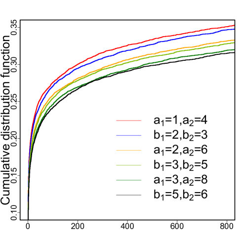
Figure 1: Empirical distribution functions of $Y_{1}$ and $Y_{2}$ with $\alpha=0.1,\ \beta=0$ (left) and $\alpha=0.1,\ \beta=-0.4$ (right).

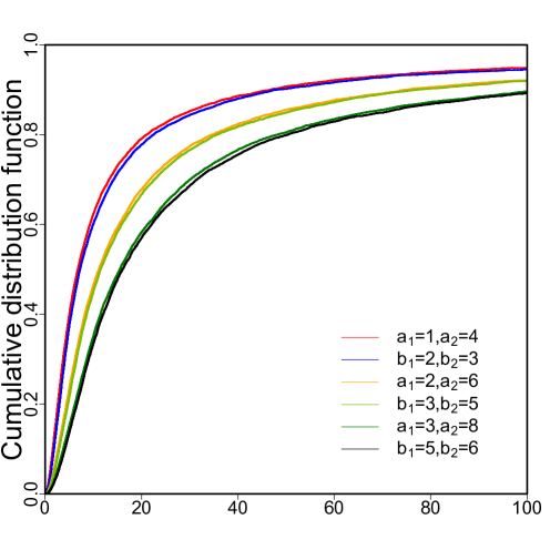
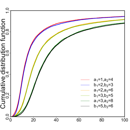
Figure 2: Empirical distribution functions of $Y_{1}$ and $Y_{2}$ with $\alpha=0.9,\ \beta=0$ (left) and $\alpha=0.9,\ \beta=0.3$ (right).

5 Concluding remarks

In this paper, we study sufficient and necessary conditions for the stochastic dominance relation (SD) across different classes of distributions. While previous studies have established (SD) for a limited set of distributions (stable distributions with tail parameter strictly less than 1 and Pareto distributions with infinite mean), we broaden the scope by proving that (SD) holds for a much richer class of distributions, denoted by $\mathcal{H}$. Moreover, if each random variable in (SD) is a compound Poisson sum, then (SD) holds if and only if the summand of the compound Poisson sum belongs to $\mathcal{H}$. We conclude the paper with some open questions.

Theorem 1 provides a sufficient condition for (SD) with the assumption that random variables are bounded from below. How far is this condition from being necessary? Moreover, as (SD) can also hold for random variables taking values on the whole real line, such as the Cauchy distribution, what is the sufficient condition of (SD) without the assumption that random variables are bounded from below?

Examples 2 and 3 show that the absolute Cauchy and the Lévy distributions belong to $\mathcal{H}$. A natural question is whether absolute stable random variables with tail parameters less than or equal to 1 and positive stable random variables also belong to $\mathcal{H}$. The absence of closed-form expressions for distribution functions in most stable distributions creates a methodological challenge in directly verifying conditions for $\mathcal{H}$, necessitating alternative analytical techniques.

Another relevant question is whether all absolute stable random variables with tail parameters less than or equal to $1$ satisfy property (SD). The answer seems to be yes based on some simulation results.

It has been shown by Chen et al., (2025) that (SD) holds for infinite-mean Pareto random variable that are positively dependent via some Clayton copula. The last question is whether such a result can be generalized for more general classes of distributions and for more general dependence structures of random variables.

Appendices

Appendix A Distributions in the class $\mathcal{H}$

In this section, we show that many infinite-mean distributions are in $\mathcal{H}$. For a distribution function $F$, we use $f$ to denote its density and let $h(x)=x^{2}f(x)$, $x\in\mathbb{R}_{+}$.

Example A.1 (Pareto distribution).

For $\alpha\in\mathbb{R}_{++}$, the Pareto distribution function is

$$F(x)=1-\frac{1}{(x+1)^{\alpha}},~~x\in\mathbb{R}_{++}.$$

If $\alpha\leq 1$, then $F$ has infinite mean. Let $h(x)=\overline{F}(1/x)=(x/(x+1))^{\alpha}$, $x\in\mathbb{R}_{+}$. Taking the second-order derivative of $h$, we have

$$h^{\prime\prime}(x)=\frac{\alpha(\alpha-2x-1)}{x^{2-\alpha}(x+1)^{2+\alpha}}.$$

If $\alpha\leq 1$, then $h^{\prime\prime}$ is concave. Thus, by Proposition 2, we have $F\in\mathcal{H}$ if $\alpha\leq 1$.

Example A.2 (Log-Pareto distribution).

The log-Pareto distribution (see p. 39 in Arnold, (2015)) has distribution function

$$F(x)=1-\frac{1}{(\log(x+1)+1)^{\alpha}},~~x\in\mathbb{R}_{++}.$$

The derivative of $h$ is

$$h^{\prime}(x)=-\frac{\alpha x}{(x+1)^{2}(\log(x+1)+1)^{\alpha+2}}\big{[}\alpha x-(x+2)\log(x+1)-2\big{]}.$$

Let

$$g(x)=\alpha x-(x+2)\log(x+1)-2,~~x\in\mathbb{R}_{+}.$$

By Proposition 2, we need $h^{\prime}(x)\geq 0$, or equivalently, $g(x)\leq 0$, such that $F\in\mathcal{H}$. As $g(0)=0$, it is sufficient to chose $\alpha$ such that $g$ is decreasing. We have

$$g^{\prime}(x)=\alpha-\frac{x+2}{x+1}-\log(x+1).$$

Thus if $\alpha\leq 2$, then $F\in\mathcal{H}$.

Example A.3 (Inverse Burr distribution).

The inverse Burr distribution is defined as

$$F(x)=\left(\frac{x^{\tau}}{x^{\tau}+1}\right)^{\alpha},~~x\in\mathbb{R}_{++},$$

where $\alpha,\tau\in\mathbb{R}_{++}$. For $x\in\mathbb{R}_{+}$,

$$h^{\prime}(x)=\alpha\tau x^{\alpha\tau}(x^{\tau}+1)^{-\alpha-2}(\alpha\tau-(\tau-1)x^{\tau}+1).$$

Hence, if $\tau\leq 1$, then $h^{\prime}(x)\geq 0$. By Proposition 2, we have $F\in\mathcal{H}$.

Example A.4 (Stoppa distribution).

For $\alpha,\beta\in\mathbb{R}_{++}$, a (location-shifted) Stoppa distribution can be defined as

$$F(x)=\left(1-\frac{1}{(x+1)^{\alpha}}\right)^{\beta},~~x\in\mathbb{R}_{++}.$$

Since a Stoppa distribution is a power transform of a Pareto distribution, by Proposition 3 (i), if $\alpha\leq 1$, then $F\in\mathcal{H}$. Power transforms have also been used to generalize Burr distributions (see p. 211 of Kleiber and Kotz (2003)).

Example A.5 (Log-Cauchy distribution).

The log-Cauchy distribution function is

$$F(x)=\frac{1}{\pi}\arctan(\log(x))+\frac{1}{2},~~x\in\mathbb{R}_{++}.$$

We have

$$f(x)=\frac{1}{x^{2}\pi}\frac{x}{(\log(x))^{2}+1}.$$

As $x/(\log(x)^{2}+1)$ is increasing in $x$, then $F\in\mathcal{H}$ by Remark 2.

Appendix B Simulation of stable distributions

We recall below the simulation procedure of standard stable distributions $S_{\alpha}(1,\beta,0)$ in Weron (1996).

• Let two random variables $V\sim U(-\pi/2,\pi/2)$ and $W\sim{\rm Exp}(1)$ be independent.

• For $\alpha\neq 1$, let

  $$X=M_{\alpha,\beta}\frac{\sin(\alpha(V-N_{\alpha,\beta}))}{(\cos(V))^{1/\alpha}}\left(\frac{1}{W}\cos\Big{(}V-\alpha(V-N_{\alpha,\beta})\Big{)}\right)^{(1-\alpha)/\alpha},$$

  where

  $$M_{\alpha,\beta}=\left[1+\beta^{2}\tan^{2}\left(\frac{\pi\alpha}{2}\right)\right]^{1/(2\alpha)},\qquad N_{\alpha,\beta}=-\frac{1}{\alpha}\arctan\left(\beta\tan\frac{\pi\alpha}{2}\right).$$

• For $\alpha=1$, let

  $$X=\frac{\pi}{2}\left[\left(\frac{\pi}{2}+\beta V\right)\tan(V)-\beta\log\left(\frac{W\cos(V)}{\pi/2+\beta V}\right)\right].$$

As $X\sim S_{\alpha}(1,\beta,0)$, one can generate samples of $X$ by first generating samples of $V$ and $W$ and then plug in the samples to the above stochastic representations of $X$.

Funding

Y. Chen is supported by the 2025 Early Career Researcher Grant from the University of Melbourne. T. Hu would like to acknowledge financial support from National Natural Science Foundation of China (No. 72332007, 12371476). Z. Zou is supported by National Natural Science Foundation of China (No. 12401625), the China Postdoctoral Science Foundation (No. 2024M753074), the Postdoctoral Fellowship Program of CPSF (GZC20232556).

Disclosure statement

No potential conflict of interest was reported by the authors.

References

- (1)
- Arab et al., (2024) Arab, I., Lando, T., and Oliveira, P. E. (2024). Convex combinations of random variables stochastically dominate the parent for a large class of heavy-tailed distributions. arXiv:2411.14926.
- Arnold, (2015) Arnold, B. C. (2015). Pareto Distributions. Second Edition. CRC Press, New York.
- Boyd and Vandenberghe, (2004) Boyd, S. and Vandenberghe, L. (2004). Convex Optimization. Cambridge university press.
- Chen et al. (2024a) Chen, Y., Embrechts, P. and Wang, R. (2024a). An unexpected stochastic dominance: Pareto distributions, dependence, and diversification. Operations Research, forthcoming.
- Chen et al., (2025) Chen, Y., Hu, T., Wang, R. and Zou, Z. (2025). Diversification for infinite-mean Pareto models without risk aversion. European Journal of Operational Research, 323(1):341–350.
- Chen and Shneer, (2024) Chen, Y. and Shneer, S. (2024). Risk aggregation and stochastic dominance for a class of heavy-tailed distributions. arXiv:2408.15033.
- Chen and Wang (2025) Chen, Y. and Wang, R. (2025). Infinite-mean models in risk management: Discussions and recent advances. Risk Sciences, 1:100003.
- de Haan and Ferreira (2006) de Haan, L. and Ferreira, A. (2006). Extreme Value Theory: An Introduction. Springer, New York.
- Denuit et al. (2005) Denuit, M., Dhaene, J., Goovaerts, M. and Kaas, R. (2005). Actuarial Theory for Dependent Risks: Measures, Orders and Models. John Wiley & Sons, West Sussex.
- Durrett, (2019) Durrett, R. (2019). Probability: Theory and Examples. Fifth Edition. Cambridge University Press.
- Embrechts et al. (1997) Embrechts, P., Klüppelberg, C. and Mikosch, T. (1997). Modelling Extremal Events for Insurance and Finance. Springer, Heidelberg.
- Embrechts et al., (2002) Embrechts, P., McNeil, A. and Straumann, D. (2002). Correlation and dependence in risk management: properties and pitfalls. In Risk Management: Value at Risk and Beyond (Eds: Dempster), pp. 176–223, Cambridge University Press.
- Ibragimov, (2005) Ibragimov, R. (2005). New majorization theory in economics and martingale convergence results in econometrics. Ph.D. dissertation, Yale University, New Haven, CT.
- Ibragimov, (2009) Ibragimov, R. (2009). Portfolio diversification and value at risk under thick-tailedness. Quantitative Finance, 9(5), 565-580.
- Ibragimov et al. (2011) Ibragimov, R., Jaffee, D. and Walden, J. (2011). Diversification disasters. Journal of Financial Economics, 99(2):333–348.
- Ibragimov and Walden, (2010) Ibragimov, R. and Walden, J. (2010). Optimal bundling strategies under heavy-tailed valuations. Management Science, 56(11):1963–1976.
- Kaas et al., (2008) Kaas, R., Goovaerts, M., and Dhaene, J. (2008). Modern Actuarial Risk Theory. Springer Science & Business Media.
- Kleiber and Kotz (2003) Kleiber, C. and Kotz, S. (2003). Statistical Size Distributions in Economics and Actuarial Science. John Wiley & Sons.
- Ma (1998) Ma, C. (1998). On peakedness of distributions of convex combinations. Journal of Statistical Planning and Inference, 70(1):51-56.
- Ma (2000) Ma, C. (2000). Convex orders for linear combinations of random variables. Journal of Statistical Planning and Inference, 84(1-2):11-25.
- Mao et al. (2013) Mao, T., Pan, X. and Hu, T. (2013). On orderings between weighted sums of random variables. Probability in the Engineering and Informational Sciences, 27(1):85-97.
- Marshall et al. (2011) Marshall, A. W., Olkin, I. and Arnold, B. (2011). Inequalities: Theory of Majorization and Its Applications. Second edition. Springer, New York.
- Müller and Stoyan, (2002) Müller, A. and Stoyan, D. (2002). Comparison Methods for Stochastic Models and Risks. Wiley, England.
- Müller, (2024) Müller, A. (2024). Some remarks on the effect of risk sharing and diversification for infinite mean risks. arXiv:2411.10139.
- Nešlehová et al., (2006) Nešlehová, J., Embrechts, P. and Chavez-Demoulin, V. (2006). Infinite mean models and the LDA for operational risk. Journal of Operational Risk, 1(1):3–25.
- Ng, (1987) Ng, C. (1987). Functions generating Schur-convex sums. General Inequalities, 5, (W. Walter, ed.), 433–438. Birkhäuser, Basel.
- Nolan (2020) Nolaen, J.P. (2020). Univariate Stable Distributions. Springer, New York.
- Pan et al. (2013) Pan, X., Xu, M. and Hu, T. (2013). Some inequalities of linear combinations of independent random variables: II. Bernoulli, 19(5A):1776-1789.
- Proschan (1965) Proschan, F. (1965). Peakedness of distributions of convex combinations. The Annals of Mathematical Statistics, 36(6):1703-1706.
- Shaked and Shanthikumar (2007) Shaked, M. and Shanthikumar, J. G. (2007). Stochastic Orders. Springer, New York.
- Weron (1996) Weron, R. (1996). On the Chambers-Mallows-Stuck method for simulating skewed stable random variables. Statistics Probability Letters, 28(2):165-171.
- Xu and Hu (2011) Xu, M. and Hu, T. (2011). Some inequalities of linear combinations of independent random variables: I. Journal of Applied Probability, 48(4):1179-1188.
- Yu (2011) Yu, Y. (2011). Some stochastic inequalities for weighted sums. Bernoulli, 17(3):1044-1053.
- Zhao et al. (2011) Zhao, P., Chan, P. S. and Ng, H. K. T. (2011). Peakedness for weighted sums of symmetric random variables. Journal of Statistical Planning and Inference, 141(5):1737-1743.
- Zhang and Cheung (2020) Zhang, Y. and Cheung, K. C. (2020). On the increasing convex order of generalized aggregation of dependent random variables. Insurance: Mathematics and Economics, 92:61-69.
- Zwet, (1964) Zwet, W. R. (1964). Convex Transformations of Random Variables. Mathematisch Centrum Amsterdam.