∎
2500 Campus Rd, Honolulu, HI, 96822
22email: qcharles@hawaii.edu 33institutetext: Pierre-Olivier Parisé 44institutetext: Université du Québec à Trois-Rivières
3351 Bd des Forges, Trois-Rivières, QC, G8Z 4M3, Canada
44email: pierre-olivier.parise@uqtr.ca
Classification of Principle 3D Slices of Filled-in Julia Sets in Multicomplex Spaces
Abstract
A generalization of the filled-in Julia set is presented using the multicomplex numbers and an algorithm is presented to visualize these sets in the tridimensional space. There are many ways to visualize these higher dimensional fractals sets on a computer. We therefore introduce an equivalence relation between 3D representations and show that, for the filled-in Julia sets associated to the polynomial , there are nine 3D slices when is an odd integer and four when is even. These results differs from the recent characterization obtained by Brouillette and Rochon in 2019 and the proofs require different arguments in the context of the filled-in Julia sets.
Keywords:
Filled Julia sets Multicomplex numbers 3D Fractals Multicomplex dynamics Tricomplex spaceMSC:
37F50 32A30 30G35 00A691 Introduction
The theory of dynamical systems is a branch of mathematics that studies the evolution of a system that follows specific rules. This discipline was initiated by H. Poincaré following his study of the three-body problem. It became popular among the public thanks to the experiments by E. Lorenz on climate models in 1963, which also gave rise to the expression “butterfly effect.” Today, this mathematical theory has become a central tool in many fields of Science and engineering Mandel1975 ; May1976 .
One branch of the theory of dynamical systems is holomorphic dynamics, which studies the dynamics generated by the iteration of differentiable functions with complex values. It arose from the work of two French mathematicians, Gaston Julia and Pierre Fatou, published between 1917 and 1920. The work of mathematicians such as B. Mandelbrot, A. Douady, and J. H. Hubbard revived researchers’ interest in this theory. Among other things, two sets in particular have attracted attention due to their remarkable properties: the filled-in Julia sets and the Mandelbrot set.
On one hand, given a polynomial function , the filled-in Julia set associated to the function is the set of such that the orbit of under , that is the sequence , where , is bounded. In this paper, we focus mainly on the filled-in Julia sets associated to the polynomials , where is an integer. These sets will be denoted by . On the other hand, the Mandelbrot set is the set of parameters such that the orbit of is bounded, that is the sequence remains bounded. It is usually denoted by .
In recent years, more and more researchers became interested in generalizing the Mandelbrot set and the filled-in Julia sets to higher dimensions. One of the pioneers in this field was A. Norton Norton1982 . He used the quaternions to render a three dimensional version of a filled-in Julia set. Many others followed Norton’s work, but the generalization that gave rise to the richer theory was obtained by Rochon rochon2000 ; rochon2003 , Garrant-Pelletier and Rochon PR2009 , and Parisé and Rochon PR2015 . They used the so-called multicomplex numbers.
Multicomplex numbers, usually denoted by or where is an integer representing the order, are a commutative generalization of complex numbers to higher dimensions that were introduced by C. Segre. They are constructed inductively with and being an isomorphic copy of the complex numbers. The main reference for multicomplex numbers is Price’s book Pr1991 . We have seen, in recent years, an explosion of articles referring to applications of the multicomplex numbers, including the generation of 3D fractals. Here is a non exhaustive list of applications of the multicomplex numbers: generalization of the Mandelbrot and filled-in Julia sets to higher dimensions Brouillette_2019 ; PR2009 ; PR2015 ; rochon2000 ; rochon2003 ; Wang2013 , generalization of some equations in physics such as the linear and non-linear Schrödinger equations and solitons B2017 ; Cen2020 ; K2023 ; rochon2004 ; TVG2017 , and generalization of complex-valued neural networks Alpay2023 . For instance, in rochon2004 , the author employed bicomplex numbers to generalize the Schrödinger equation. As a result, he was able to unify two fundamental equations in physics—the Schrödinger equation and the Klein-Gordon equation—within a single framework.
When , the set is the set of bicomplex numbers and these numbers take the form
where , with and with . Tricomplex numbers have a similar representation but with components and in general, a multicomplex numbers have a similar representation but with components. Therefore a Mandelbrot set or a filled-in Julia set generalized using multicomplex numbers can’t be visualize when the order of the multicomplex numbers used is greater than or equal to . Garrant-Pelletier and Rochon PR2009 solved this problem by considering three dimensional subspaces of the multicomplex numbers to visualize the Mandelbrot set and the theory was then further generalized by Parisé and Rochon PR2015 , and improved by Brouillette and Rochon Brouillette_2019 .
There is a remarkable phenomena that occurs in the case of the multicomplex Mandelbrot set. Many visualization through different three dimensional subspaces, called principal 3D slices, give rise to the same set and therefore the multicomplex Mandelbrot set exhibits internal symmetries at lower dimensions. In particular, Brouillette and Rochon have shown the following important result.
Theorem 1.1
Let and . Then any principal 3D slices of the multicomplex Mandelbrot set can be obtained from a principal 3D slices of the tricomplex Mandelbrot set.
No such result exists for the multicomplex filled-in Julia sets, except some rudimentary results on the bicomplex filled-in Julia sets obtained in Wang2013 . The main goal of this paper is to therefore introduce the multicomplex filled-in Julia sets associated to the polynomials and to prove a quantitive result on the principal 3D slices which is the quantitative analogue of Brouillette and Rochon’s result. Our main result reads as followed:
Theorem 1.2
Let , be integers, and be a real number.
-
1.
If is an even integer, then the multicomplex filled-in Julia set has principal 3D slices for any .
-
2.
If is an odd integer and , then the multicomplex filled-in Julia set has principal 3D slices.
-
3.
If is an odd integer and , then the multicomplex Mandelbrot set has principal 3D slices when and principal 3D slices for any .
The paper is structured as followed. In Section 2, we introduce the algebra of multicomplex numbers. In Section 3, we introduce the precise definition of the filled-in Julia set and give some of their basic properties. In Section 4, we introduce the multicomplex filled-in Julia sets and present some of their elementary properties. In Section 5, we define what is a principal 3D slices of a filled-in Julia set. In section 6, we introduce our new equivalence relation between the sets of principal 3D slices of a filled-in Julia set and prove a list of preliminary results needed in the proof of our main result. Finally, in Section 7, we prove our main result on the number of principal 3D slices of the multicomplex filled-in Julia set.
2 Preliminary on Multicomplex Numbers
The objective of this section is to introduce the definition of multicomplex numbers, their basic algebraic operations, and their topology.
2.1 Multicomplex Numbers
The Multicomplex number are a generalization of the complex numbers to higher dimensions. The original reference to multicomplex numbers is the book of Price Pr1991 . For recent and succinct introductions to multicomplex numbers, the reader is also directed to the papers Brouillette_2019 ; doyon2022 . Our presentation will mainly follow the paper doyon2022 .
The set of Multicomplex numbers is denoted by for any , where is an integer representing the order. For , we set , for , we set with , the usual imaginary unit, and for any integer , the element of are defined recursively as followed:
where the symbol is an imaginary unit such that and . Note that with this definition, the usual set of complex numbers corresponds to the set .
Given two multicomplex numbers and , the operation of addition, denoted , of two multicomplex numbers is defined as followed:
where the addition in each component is the addition defined in and the operation of multiplication, denoted by , between two multicomplex numbers is defined as
where the operations in each components are the addition and multiplication coming from . One can show that the triplet forms a commutative unitary ring (see, for instance, Pr1991 ).
When , we obtain the set of complex numbers which, compared to all other cases of multicomplex numbers, is a commutative field. When , we obtain the set of bicomplex numbers and each bicomplex number can be written down as , where . Describing each component of the bicomplex number as and , where , we can rewrite as
Distributing the number and relabeling the index of each real component, we obtain
We can therefore write any bicomplex number as a -linear (complex linear) combination of the units and or as a -linear (real linear) combination of the units , , , and .
The decomposition of a bicomplex number as a real-linear combination of units can be generalized to any multicomplex numbers. Let be the set of all units of the form , where . For instance, we have
From combinatorial considerations, we can show that the number of elements of is .
Within the set , there are units that square to or to . An imaginary unit is a unit having the property that and a hyperbolic unit is a unit that have the property that and . Combinatorial considerations implies that the number of imaginary units in is and the number of hyperbolic units in is . For more details on hyperbolic units, the reader is referred to doyon2022 , where the authors found more imaginary and hyperbolic units in the set of multicomplex numbers. For this paper, however, only the set will be considered. Therefore, we can decompose a multicomplex number as
where for any .
We presented the example of a bicomplex numbers. Another important example is the set of tricomplex numbers that we will use later in the paper as our optimal space for the 3D slices of the Filled-in Julia sets. Any tricomplex number can be written down as a real-linear combination of the units from the set as followed:
where for . For reference later in the paper, we set , , , and .
2.2 Idempotent Representations
Define the multicomplex numbers and , for , as followed:
Given , it is easy to see that
Since , we obtain
This is called the idempotent representation of a multicomplex number. We set and and write the idempotent representation of a multicomplex number as followed
Because , , and , we obtain the following properties of the idempotent representation.
Theorem 2.1
Let and be two multicomplex numbers and be an integer. Then
-
1.
.
-
2.
.
-
3.
, for any integer .
Using the idempotent representation we can defined an operation similar to the Cartesian product of two sets.
Definition 1
Let , for . The set is called an -Cartesian product determined by two sets and if the following holds
2.3 Norm
The norm of a multicomplex number is defined recursively as the following quantity:
where . It can be shown that the expression of the norm of a multicomplex number can be written down in terms of the idempotent components in the idempotent representation of a multicomplex number:
where .
The topology used on is the one induced by the metric . The open balls are the set . As a consequence, the -cartesian product preserved closedness, compactness, openness, and connectedness of sets, that is
-
1.
If and are closed sets in , then the set is closed in .
-
2.
If and are compact sets in , then the set is compact in .
-
3.
If and are open sets in , then the set is open in .
-
4.
If and are connected sets, then the set is a connected set.
3 Preliminaries on the Filled-in Julia Sets in the Complex Plane
In this section, we define the Filled-in Julia sets, denoted by , over the complex plane . We will show some basic properties of the set . These properties will be essential to draw pictures of its generalization to the bicomplex and tricomplex spaces.
3.1 Definition
For a fixed complex number , the filled-in Julia set associated to the polynomial function is defined as followed:
Here the notation stands for the -th iterate of the function at , meaning when and when .
3.2 Basic Properties
The first important property of the complex Filled-in Julia sets is the fact that they are compact subsets of the complex plane. We can in fact identify exactly the radius of the disk containing a filled-in Julia set.
Theorem 3.1
Let . Then is a compact set. In particular, we have that , where .
Proof
The fact that is a compact subset of the complex plane is a known fact from the theory of holomorphic dynamics. A reference for this result is (F2014, , Theorem 14.2).
We will prove the second part of the theorem. Let be as in the statement of the theorem. We will show that , which is equivalent to the statement we want to show.
Assume that . Then and
where, in the second inequality, we used the fact that . Since , then for some positive real number . This implies that
Recall Bernouilli’s inequality for any and . Set and , then we obtain the following inequality:
Using the fact that , we have that and we obtain the following lowerbound:
Also, since and , we have that and this means
Therefore, we obtain
Assume that for some integer . Then, we have
Hence, by the Principle of Induction, we just proved that if , then
Since , then and therefore the sequence is unbounded. This means . This concludes the proof. ∎
From the above proof, we can extract an important lemma that will be at the core of the justification of the algorithm to draw filled-in Julia sets.
Lemma 1
Let and . If there exists a positive integer such that , then there is some positive real number such that for any integer .
Proof
Assume that for some positive integer . Let be such that . Reproducing the proof of the preceding Theorem with replaced by , we can show that
This is the base case . Assuming that , we then have
which establishes the induction step. The Principle of Induction then concludes the proof. ∎
3.3 An Algorithm
We can now prove the following theorem which gives an algorithm to draw pictures of filled-in Julia sets in the complex plane.
Theorem 3.2
Let and . The following assertions are equivalent:
-
1.
.
-
2.
for any positive integer .
Proof
If for any positive integer , then the sequence is bounded and hence . This proves the implication (2) (1).
To prove the implication (1) (2), we will prove the contrapositive. Assume that there is a positive integer such that . By Lemma 1, we deduce that for some , we have
Since , then and hence . The contrapositive of the implication (1) (2) is therefore true and hence the implication is also true. ∎
From Theorem 3.2, we can construct an algorithm to draw a filled-in Julia set in the complex plane. Fix , and . For each complex number in the square ,
-
1.
Compute the -th iterate , for .
-
2.
At every iteration, compute and verify the following conditions:
-
(a)
If for some , then assume that and assign a color to the number .
-
(b)
if for every , then assume that and assign a different color than the one chosen in (a) to the number .
-
(a)
4 Higher Dimensional Filled-in Julia Sets
We now generalize the filled-in Julia sets to higher dimensions. This was done previously in PR2009 for the polynomial . We generalize it here for the polynomial .
Throughout this section, the function will be the polynomial , where and are positive integers greater than or equal to . As we used in the previous section, the -th iterate of the function is defined as when and when .
4.1 Multicomplex Filled-in Julia Sets
The multicomplex filled-in Julia set associated to the polynomial , with is defined as followed.
Definition 2
Let . The multicomplex filled-in Julia set associated to is denoted by and
When , we recover the definition of the filled-in Julia sets in the complex plane. Two other cases are of importance in this paper:
-
1.
When , is the set of bicomplex numbers. We therefore obtain the bicomplex version of the filled-in Julia sets denoted by (see rochon2003 for the case ).
-
2.
When , is the set of tricomplex numbers. We therefore obtain the tricomplex version of the filled-in Julia sets denoted by (see PR2009 for ).
The case of the tricomplex numbers will be particularly important for our main result.
4.2 Basic properties
Some of the basic properties stated in this section were already mentioned, without proofs, in BPR2019 . For the sake of the reader, we provide the complete proofs of these results here.
Using the idempotent representation of a multicomplex number, we can obtain the following important decomposition of a multicomplex filled-in Julia set.
Theorem 4.1
Let be an integer and , with the idempotent components of . Then we have
Proof
Let and be as in the statement of the theorem. Using the idempotent representation, for any and , we have
and therefore
It immediately follows from this last equality that the sequence is bounded if and only if the two sequences and are bounded. Hence, if and only if and if and only if . This completes the proof. ∎
We collect below two subcases of the previous result.
-
1.
When , we have , where .
-
2.
When , we obtain , where .
The next result will be important in the next section to draw pictures of the higher dimensional filled-in Julia sets.
Theorem 4.2
Let be an integer and . Let . Then the following assertions are equivalent:
-
1.
.
-
2.
for every integer .
Proof
The proof will be by induction on . The case was proved in the previous section and is Theorem 3.2.
Now, assume that the statement of the theorem is true for , that is, for any , (1) is equivalent to (2). We have to prove that (1) is equivalent to (2) for . Let be expressed in their idempotent representation:
where . To simplify the notations, we set , , , and .
Assume that for any integer . Then, from the definition of the filled-in Julia set, . So, (2) implies (1).
Assume that . Then, and by Theorem 4.1. By the induction hypothesis, we get
for any integer . Using the fact that for any integer , we have
and using the expression of the norm in terms of the idempotent components, we get
Hence and the statement is proved for .
By the Principle of Mathematical Induction, the proof is complete. ∎
5 Visualization through 3D Slices
In this section, we will be interested in visualizing the higher dimensional version of the filled-in Julia sets over the multicomplex numbers. Thoughout this section, the letter is used to denote a positive integer greater than or equal to . We also let be a positive integer greater than or equal to .
In order to visualize the multicomplex filled-in Julia sets, we define the concept of a 3D slice. We will first need to define (real) vector subspaces of .
Definition 3
Let be distinct. We define the following (real) vector subspace of :
For instance, if , then we have . The principal units can therefore be real, imaginary, or hyperbolic in nature. We can now define a principal 3D slices of a multicomplex filled-in Julia set.
Definition 4
Let and let be distinct. A principal 3D slice of the filled-in Julia set is defined as followed:
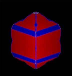
From Theorem 4.2, we can construct an algorithm to visualize multicomplex filled-in Julia sets in 3D for . Fix , and . Fix also three distinct principal units . For each multicomplex number , where ,
-
1.
Compute the -th iterate , for .
-
2.
At every iteration, compute and verify the following conditions:
-
(a)
If for some , then assume that and assign a color to the number .
-
(b)
if for every , then assume that and assign a different color than the one chosen in (a) to the number .
-
(a)
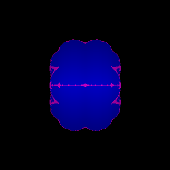
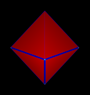
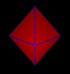
See Figure 1 for two examples of principal 3D slices visualized using the above algorithm. More powerful methods exist to visualize principal 3D slices, see Pierre_Guillaume_Dominic_2019 .
6 Definitions and Preliminaries for the Characterization of 3D slices
In this section, we present the main tools needed to obtain our main result on the characterization of the principal 3D slices.
6.1 An equivalent relation
The next definition introduces the space of iterates.
Definition 5
Let and . The (real) vector subspace of iterates is defined as followed:
When we write ”characterization of the 3D slices”, what we mean is to find the equivalent classes of the following equivalent relation.
Definition 6
Let . Let be distinct principal units and let be three other distinct principal units111The units , , might be the same as the units , , . The only important fact is that you choose a set of three different units.. Define and . The 3D slices and are equivalent, denoted by if and only if there exists a linear bijective application such that
-
1.
, for any .
-
2.
, for any .
Condition (1) guarantees the first iterates with a starting point in and in respectively are the same. This is especially important if or .
Condition (2) guarantees the subsequent iterates behave in the same way. Indeed, an induction argument shows that
Since is a bijective linear map, the inverse is also a bijective map and and are continuous. Therefore, for and , the sequence is bounded if and only if the sequence is bounded.
Notice that Definition 6 is similar to Definition 5 in Brouillette_2019 . However in general the map can’t be applied directly to to obtain because it might not be defined on the subspaces and . In opposition to what was just said, the map in the definition in Brouillette_2019 is always defined on the subspaces and . Therefore, our definition covers both cases, the multicomplex filled-in Julia sets and the multicomplex Mandelbrot sets.
Theorem 6.1
Let . The relation is an equivalent relation on the set of 3D slices of , meaning that is a reflexive, symmetric, and transitive binary operation on the family of principal 3D slices.
Proof
We have to show that the binary operation is reflexive, symmetric, and transitive.
-
(a)
Let be a principal 3D slice. Let and let be the identity map . Then, all conditions in the definition of the relation are automatically verified and .
-
(b)
Let and be two principal 3D slices such that
Then there is a bijective map , where and , such that
-
(1)
, for any .
-
(2)
, for any .
Let . Therefore, and from the condition (1), we get
Also, writing , from condition (2), we obtain
and taking the inverse of on each side, we get
Hence, satisfies the two conditions in Definition 6 and .
-
(1)
-
(c)
To simplify the notation, we will omit the units in the 3D slices. Let , , and be three principal 3D slices such that and . Then there exist two bijective maps and such that conditions (1) and (2) from Definition 6 are satisfied. Then it is not hard to see that the map defined by satisfies conditions (1) and (2) of Definition 6. Hence, and this ends the proof. ∎
6.2 Characterization of the space of iterates
The goal now is to find simple expressions for the space of iterates. To do so, we introduce the following (real) vector subspaces.
-
1.
.
-
2.
.
-
3.
.
If one of the , , is equal to , then we will always assume, without loss of generality, that . We can now prove the following results.
Theorem 6.2
Let . Then
-
1.
The space is closed under multiplication.
-
2.
If or for some index , then .
-
3.
The space is closed under multiplication.
-
4.
If and , then .
-
5.
If , then .
-
6.
If or for some index , then .
Proof
See (Brouillette_2019, , Lemma 2) for the complete proof of part (1).
To show (2), assume first that . From the definition of both subspaces, we get the equality . Now, assume, without loss of generality, that . From that additional assumption, we see that with , with , with and with . Therefore, we get
and hence if and only if .
To show (3), it is sufficient to show that every multiplication of the basis elements generating is again one of the basis elements. This can be achieved by constructing the following multiplication table:
Hence, is closed under multiplication.
To show parts (4) and (5), we use the same strategy that was used to show (3). We therefore omit their proofs and this concludes the proof of the statement. ∎
We can now prove the following result regarding the precise expression of the vector subspaces .
Theorem 6.3
Let and . Then
-
1.
If is even, then .
-
2.
If is odd and if , then .
-
3.
If is odd and if , then
-
(a)
if or if for some distinct .
-
(b)
otherwise.
-
(a)
Proof
We first start by showing part (1). Assume that is even, so that for some positive integer , and that . We have to show an equality between two sets.
We start by showing the inclusion . For the rest of this part, let with where . We will prove using induction that for any integer . The first iterate is . We will prove with an induction on that . Starting with , we have
Since , , and , we deduce that . Now assume for some , we have . Then, we have
From Theorem 6.2 part (3), the space is closed under multicomplex multiplication. We know that and, from the induction hypothesis, we have . Therefore and hence . Adding the number , we have just shown that .
Now assume that for some integer . We want to show that . The expression of the -th iterate is
From Theorem 6.2 part (3), the space is closed under multicomplex multiplication. Hence, we must have that because from the induction hypothesis. Hence, . This concludes the induction on and the proof of .
We now want to prove the other direction, that is . To do that, we will show that each basis elements (, , , ) is a linear combination of some iterates. Setting implies that
where . Hence, . To show that the other basis elements are a linear combination of some iterates, we will use a similar trick from Brouillette and Rochon’s paper (see the proof of (Brouillette_2019, , Lemma 3)). For with and , we have
and splitting the sum over the that are even and the that are odd, we get
The last equation can be rewritten as , where and are real-valued polynomials of degree and respectively. Since a polynomial has finitely many roots, we may choose a number (that depends on and ) such that . We then obtain
and using the fact that , we can rewrite the last expression as followed
Therefore, we obtain , this finishes the proof of part (1).
Now we show part (2). Our goal is to show that for odd and , we have . We first show that . Consider and for . We will prove by induction on that . For , we have
From part (1), we know that for any . Since , it follows from Theorem 6.2 part (4) that
Hence, . Now assume that for some positive integer . Then we have
Using Theorem 6.2 part (5), we have since, from the induction hypothesis, . From Theorem 6.2 part (3), the set is closed under multicomplex multiplication and therefore . Now, using Theorem 6.2 part (4), we obtain that because . Hence, we obtain . Hence, by the Principle of Mathematical Induction, the proof of the inclusion is completed.
We now want to show that . We will do this by expressing each basis element , , , and as a linear combination of iterates. Let with , then we have
Hence, , where . To express the other element as a linear combination of iterates, we will adapt the trick used earlier that comes from Brouillette and Rochon’s paper (see the proof of (Brouillette_2019, , Lemma 3)). Consider with . Then we have
Splitting the summation over the different parities of the integers and , we obtain
which can be rewritten as
where , , , and are polynomials in . Since polynomials have only finitely many roots, we can choose a value such that . Therefore, we obtain
This shows that every basis element can be rewritten as a linear combination of iterates and therefore .
Finally, we show part (3). Assume that is odd, but . The proof of part (a) is similar to the proof of parts (1) and (2). We will therefore focus on the proof of part (b). We want to show that .
We start by showing that . Let . We will do an induction on in . Let so that . From the proof of the base case in part (2), we know that . This implies that . Now assume that the claim is true for some integer , which means that . From the definition of the iterates, we have . From the Induction Hypothesis, we have . From Theorem 6.2 part (1), the subspace is closed under multiplication and we then get . Hence, and we conclude that .
We now show the reverse inclusion by showing that each basis element of can be written down as a linear combination of some iterates. Notice that and since , we have . Let for so that
and hence with . Let so that, from the calculations performed at the end of the proof of part (2), we get
with . To find the linear combination to express the other basis elements, namely, , , and , we adapt for a second time the trick from Brouillette and Rochon’s paper (see the proof of (Brouillette_2019, , Lemma 3)). Let with and define . Then, using the binomial theorem, we get
where and are polynomials in . Using this expression for , we can now write
Splitting the sums over the parity of and , we get
which can be rewritten as
where , , , and are polynomials in the variable . Since any polynomial has finitely many roots, we can choose a value of () that avoids the roots of and therefore . Letting , we get
and after isolating , we get
Similarly, we can write and as a linear combinations of iterates. This shows the inclusion and completes the proof of the theorem. ∎
7 Characterization of 3D slices
The statement of Theorem 6.3 indicates that a space of iterates behave differently depending on the parity of the integer and on the nature of the principal units used. We will therefore start by proving our main result on the classification of principal 3D slices when is an even integer and then prove the result when is an odd integer.
7.1 Main result for even powers
Before proving our first main result, we make several assumptions on the principal units. It is rather easy to see that where is a permutation of the symbols , , . The order of the units is therefore not important and we can choose a specific ordering.
We choose the following ordering for a triplet of principal units , , : has priority for the first position over imaginary units and hyperbolic units; imaginary units have priority for the second position over hyperbolic units. When all of the principal units are of the same nature, we then put them in increasing index.
For instance, the 3D slices , , , and , , are all equivalent to . Another example is the group of 3D slices , , , , , and . They are all equivalent to . Without loss of generality, we will therefore assume that the principal units follow this choice of ordering.
Our first result concerning the characterization of the 3D slices of the filled-in Julia sets goes as followed. This is part 1 of Theorem 1.2
Theorem 7.1
Let be an integer and . If is an even positive integer, then there are principal 3D slices.
Proof
Let and choose such that , , and . Such units always exist if . We will show that .
When is even, from Theorem 6.3 part (1), we have and . So define the linear map on the basis elements and extend it linearly: , , , and . Clearly is a bijective linear map.
A way to show that is to show that . In fact, we can show that for any . Let and . Then, we have
By linearity of and the assumptions on the squares of each principal units, we get
An induction argument on then shows that . Using this property, we get
Hence, condition (2) in Definition 6 is satisfied.
It remains to show that condition (1) in Definition 6 is satisfied, since and . For for and for , we calculate
Applying to the last equality and using linearity, we obtain
and since , and , we conclude that
An induction argument on then implies that which means that
for arbitrary . Hence, condition (2) of Definition 6 is satisfied and the two 3D slices are equivalent.
We therefore only need to study the sign of the squares of the principal units. There are choices for each principal units, that is and . Since the order of the selection of the principal units is not important, this gives us choices:
-
1.
. In this case, all principal 3D slices are equivalent to .
-
2.
and . In this case, all principal 3D slices are equivalent to .
-
3.
and . In this case, all principal 3D slices are equivalent to .
-
4.
. In this case, all principal 3D slices are equivalent to .
This ends the proof. ∎
We notice that all principal 3D slices are obtained from units in the set of tricomplex numbers. We therefore obtain the following consequence of our result.
Corollary 1
Let et be integers and . For any principal 3D slice of , there exists a principal 3D slice of such that .
7.2 Main result for odd powers
We now treat the case when is an odd integer and . The case is treated very similarly as in the previous section. This comes from the fact that when , the space of iterates is equal to and this characterization of the space of iterates is valid for any choice of principal units. We therefore end up with the same characterization as in the even case and this proves part 2 of 1.2.
Theorem 7.2
Let be an odd integer and . Then there are distinct principal 3D slices.
It remains to prove part 3 of Theorem 1.2, that is when .
Theorem 7.3
Let be an odd integer and . Then there are distinct principal slices when and distinct principal 3D slices when .
Proof
Assume that is an odd integer and . Let and choose such that , , and . Such units always exist if . We will show that , but under additional assumptions on the principal units. We therefore split the proof into cases.
-
1.
Assume that . Theorem 6.3 part (3a) implies that . Therefore, assume further that . Define on the basis elements and by linearity: , , , and . In a very similar way as in the proof of Theorem 7.1, we can show that for any so that for any . Hence, we get . This implies that because condition (1) in Definition 6 is automatically verified from the fact that condition (2) is satisfied and and . There are therefore three cases:
-
(a)
. In this case, all 3D slices are equivalent to .
-
(b)
and . In this case, all 3D slices are equivalent to .
-
(c)
. In this case, all 3D slices are equivalent to .
-
(a)
-
2.
Assume that , but . Theorem 6.3 part (3a) implies that . Therefore, assume further that . Define on the basis elements and extend it by linearity: , , , and . In a very similar way as in the proof of Theorem 7.1, we can show that for any so that for any . Hence, we get . This implies that because condition (1) in Definition 6 is automatically verified from the fact that condition (2) is satisfied and and . Since , the nature of the principal units and forces a specific type for . This gives three cases:
-
(a)
. In this case, . Hence is an hyperbolic unit and all 3D slices are equivalent to .
-
(b)
and . In this case, . Hence is an imaginary unit and all 3D slices are equivalent to .
-
(c)
. In this case, is a hyperbolic unit. Therefore, all 3D slices are equivalent to . This is case (b).
-
(a)
-
3.
Define by the following formula:
In a very similar way as in the proof of Theorem 7.1, we can show that for any so that for any . Hence, we get . This implies that . This gives four cases:
-
(a)
. This case is impossible when because all hyperbolic units are such the product of two is equal to the third. For , choose , , and . Then all 3D slices are equivalent to that particular 3D slice .
-
(b)
and . In this case, choose , , and , then all 3D slices are equivalent to .
-
(c)
and . In this case, choose , , and , then all 3D slices are equivalent to .
-
(d)
. In this case, choose , , and , then all 3D slices are equivalent to .
After compiling all the possible cases, we see that when , there are principal 3D slices and when , there are principal 3D slices.
-
(a)
This concludes the proof. ∎
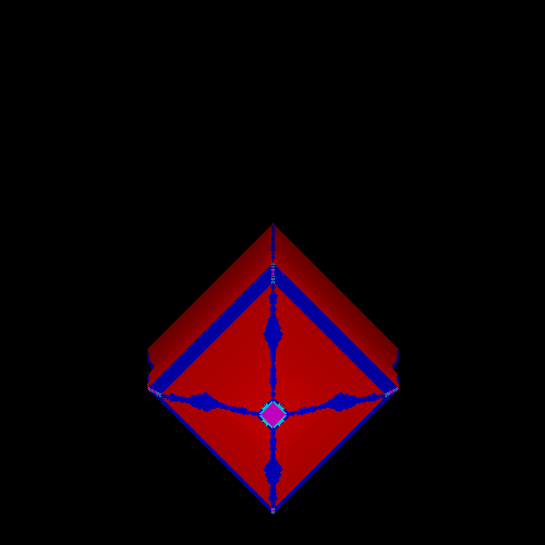
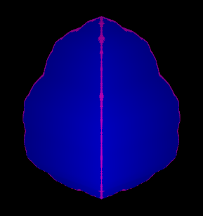
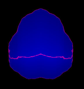
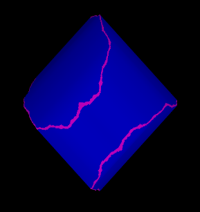
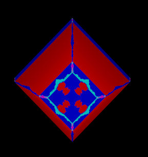
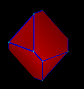
In figure 2, we illustrate all the possible principle 3D slices when , and .
8 Conclusion
In summary, we have introduced the multicomplex numbers and their topology to investigate the filled-in Julia sets in higher dimensions. The multidimensional version of the filled-in Julia sets was introduced in Section 4 and an algorithm was presented to visualize them with a computer. In Section 6, we introduced an equivalence relation as our basis for the analysis of the principal 3D slices. We then proved our main results on the number of 3D slices of the multicomplex filled-in Julia set in section 7.
As a possible future direction of work, it would be interested to investigate in more details each equivalent classes obtained in our characterization. For instance, based on preliminary computer explorations, the principal 3D slice seems to always be an octahedron for any values of . Is that always the case? Some further mathematical investigations are necessary to elucidate this question.
References
- (1) Alpay, D., Diki, K., Vajiac, M.: A note on the complex and bicomplex valued neural networks. Appl. Math. Comput. 445, Paper No. 127864, 12 (2023)
- (2) Banerjee, A.: On the quantum mechanics of bicomplex Hamiltonian system. Ann. Physics 377, 493–505 (2017)
- (3) Brouillette, G., Parisé, P.O., Rochon, D.: Tricomplex distance estimation for filled-in julia sets and multibrot sets. International Journal of Bifurcation and Chaos 29(06), 1950085 (2019). DOI 10.1142/S0218127419500858. Preprint
- (4) Brouillette, G., Parisé, P.O., Rochon, D.: Tricomplex Distance Estimation for Filled-In Julia Sets and Multibrot Sets. International Journal of Bifurcation and Chaos 29(06), 1950085 (2019). DOI 10.1142/s0218127419500858. URL http://dx.doi.org/10.1142/S0218127419500858
- (5) Brouillette, G., Rochon, D.: Characterization of the Principal 3d Slices Related to the Multicomplex Mandelbrot Set. Advances in Applied Clifford Algebras 29(3) (2019). DOI 10.1007/s00006-019-0956-1. URL http://dx.doi.org/10.1007/s00006-019-0956-1
- (6) Cen, J., Fring, A.: Multicomplex solitons. J. Nonlinear Math. Phys. 27(1), 17–35 (2020)
- (7) Doyon, N., Parisé, P.O., Verreault, W.: Counting involutions on multicomplex numbers (2022). URL https://arxiv.org/abs/2211.13875
- (8) Falconer, K.: Fractal geometry, third edn. John Wiley & Sons, Ltd., Chichester (2014). Mathematical foundations and applications
- (9) Garant-Pelletier, V., Rochon, D.: On a generalized Fatou-Julia theorem in multicomplex spaces. Fractals 17(3), 241–255 (2009). DOI 10.1142/S0218348X09004326. URL https://doi.org/10.1142/S0218348X09004326
- (10) Köplinger, J.: Phenomenology from Dirac equation with Euclidean-Minkowskian “gravity phase”. Internat. J. Theoret. Phys. 62(2), Paper No. 35, 23 (2023)
- (11) Mandelbrot, B.: Les objets fractals. Flammarion, Editeur, Paris (1975). Forme, hasard et dimension, Nouvelle Bibliothèque Scientifique
- (12) May, R.M.: Simple mathematical models with very complicated dynamics. Nature 261(5560), 459–467 (1976)
- (13) Norton, A.: Generation and display of geometric fractals in 3-d. SIGGRAPH Comput. Graph. 16(3), 61–67 (1982). DOI 10.1145/965145.801263. URL https://doi.org/10.1145/965145.801263
- (14) Parisé, P.O., Rochon, D.: A study of dynamics of the tricomplex polynomial . Nonlinear Dynam. 82(1-2), 157–171 (2015). DOI 10.1007/s11071-015-2146-6. URL https://doi.org/10.1007/s11071-015-2146-6
- (15) Price, G.B.: An introduction to multicomplex spaces and functions, Monographs and Textbooks in Pure and Applied Mathematics, vol. 140. Marcel Dekker, Inc., New York (1991)
- (16) Rochon, D.: A generalized mandelbrot set for bicomplex numbers. Fractals 08(04), 355–368 (2000)
- (17) Rochon, D.: On a generalized fatou-julia theorem. Fractals 11(03), 213–219 (2003). DOI 10.1142/S0218348X03002075
- (18) Rochon, D., Tremblay, S.: Bicomplex quantum mechanics. I. The generalized Schrödinger equation. Adv. Appl. Clifford Algebr. 14(2), 231–248 (2004)
- (19) Theaker, K.A., Van Gorder, R.A.: Multicomplex wave functions for linear and nonlinear Schrödinger equations. Adv. Appl. Clifford Algebr. 27(2), 1857–1879 (2017)
- (20) Wang, X.y., Song, W.j.: The generalized M-J sets for bicomplex numbers. Nonlinear Dynam. 72(1-2), 17–26 (2013)