StablePCA: Learning Shared Representations across Multiple Sources via Minimax Optimization

Abstract

When synthesizing multisource high-dimensional data, a key objective is to extract low-dimensional feature representations that effectively approximate the original features across different sources. Such general feature extraction facilitates the discovery of transferable knowledge, mitigates systematic biases such as batch effects, and promotes fairness. In this paper, we propose Stable Principal Component Analysis (StablePCA), a novel method for group distributionally robust learning of latent representations from high-dimensional multi-source data. A primary challenge in generalizing PCA to the multi-source regime lies in the nonconvexity of the fixed rank constraint, rendering the minimax optimization nonconvex. To address this challenge, we employ the Fantope relaxation, reformulating the problem as a convex minimax optimization, with the objective defined as the maximum loss across sources. To solve the relaxed formulation, we devise an optimistic-gradient Mirror Prox algorithm with explicit closed-form updates. Theoretically, we establish the global convergence of the Mirror Prox algorithm, with the convergence rate provided from the optimization perspective. Furthermore, we offer practical criteria to assess how closely the solution approximates the original nonconvex formulation. Through extensive numerical experiments, we demonstrate StablePCA’s high accuracy and efficiency in extracting robust low-dimensional representations across various finite-sample scenarios.

Keywords: Matrix factorization, Multi-source analysis, Group distributionally robust learning, Fantope relaxation, Mirror prox algorithm.

1 Introduction

The integrative representation of high-dimensional data matrices from multiple sources has become a foundational challenge in modern data science, driven by the need to synthesize heterogeneous datasets such as gene expression profiles measured in multiple batches and electronic health records (EHRs) collected in different hospitals. A critical challenge lies in factorizing heterogeneous feature matrices with a unified rule while mitigating source-specific biases. Traditional integrative matrix factorization (MF) and principal component analysis (PCA) methods prioritize minimizing the average reconstruction error over the sources, which may suffer from lack of generalizability due to dominant patterns in specific subsets, systematic biases such as batch effects, and unfairness to certain subgroups.

For instance, batch effects in scRNA-seq stem from technical variations such as sequencing platforms, reagents, or protocols and confound biological signals. In the representation learning of the scRNA sequence data, these artifacts could artificially separate identical cell types, causing bias in the annotation of cell type and differential gene expression studies [27]. Similar issues occur in histopathology studies over multiple hospitals, where artifacts in image preparation introduce spurious and non-biologically relevant signals [11]. Pooling and averaging over multiple batches seems a plausible way to correct for batch effects. However, this strategy is based on the questionable assumption that the biases of multiple sources are “centered around zero” rather than being skewed or imbalanced across the batches, as is more frequently seen in practice. As a result, the pooled empirical risk minimization (ERM) method fails to attain desirable performance in batch effect correction [11]. As another example, multi-source representation learning is crucial for clinical knowledge extraction leveraging pointwise mutual information (PPMI) matrices from EHR [12, 16]. In this case, simply averaging over the pooled data from different institutions or sub-populations could cause lack of generalizability or fairness as dominant groups tend to dictate the process of factor extraction.

1.1 Our results and contributions

In this work, we propose Stable Principal Component Analysis (StablePCA), a distributionally robust framework designed to capture the shared principal directions across multiple sources. In Figure 1 of Section 2.3, we illustrate that our proposal effectively captures the principal components common to heterogeneous data obtained from multiple domains, motivating the designation of our method as StablePCA.

We borrow ideas from Group Distributionally Robust Optimization (Group DRO) [13, 23] to model potential distributional shifts among multiple sources and define an uncertainty set comprising all mixtures of the source populations. StablePCA is formulated as a minimax optimization problem aiming to minimize the worst-case approximation risk over this uncertainty set. Furthermore, in practical scenarios, domain experts may possess prior knowledge about plausible mixtures of source populations. The StablePCA framework naturally incorporates such prior information into the construction of the uncertainty set.

A primary challenge in solving StablePCA arises from the nonconvexity associated with the fixed-rank constraint set. To address this issue in the adversarial learning context, we employ a Fantope relaxation, enabling a convex reformulation of the original minimax StablePCA problem. We further establish a sufficient condition under which the optimal value of the relaxed Fantope problem coincides with that of the original nonconvex formulation.

We devise a Mirror Prox algorithm with optimistic gradients to efficiently solve the relaxed StablePCA problem. Standard gradient descent ascent methods for minimax optimization typically suffer from suboptimal convergence rates and require computationally expensive projection steps, especially when operating over non-Euclidean geometries such as the Fantope [6]. In contrast, the Mirror Prox algorithm is specifically tailored for constrained minimax problems involving non-Euclidean constraints, avoiding costly projection operations while achieving faster convergence rates [5, 18]. Building upon this, we derive explicit closed-form updates for each iteration of the Mirror Prox algorithm, ensuring efficient implementation without auxiliary optimization procedures. We establish theoretical convergence guarantees, demonstrating that the proposed Mirror Prox algorithm globally converges to the optimal solution of the relaxed StablePCA problem. Furthermore, we provide practical criteria to help evaluate how well the solution approximates the original nonconvex problem.

Lastly, we conduct simulation studies to validate the effectiveness of StablePCA. The results demonstrate that StablePCA consistently outperforms standard baselines under both in-distribution and out-of-distribution scenarios. Empirically, we observe that the gap between the relaxed Fantope formulation and the original problem is nearly negligible, indicating that our solution closely approximates the original minimax optimization of multi-source PCA with the nonconvex constraint.

1.2 Related literature

This section further reviews relevant research and highlights how our proposed method differs from or builds upon existing works.

Group DRO. Group DRO has been extensively studied in supervised learning for constructing generalizable prediction models across multiple source domains [23, 13, 31]. The recent work [32] studied the optimal sample size of Group DRO in the online learning scenario, while [1] extended Group DRO to semi-supervised learning settings. In contrast to these works, which focus on prediction tasks, our method addresses the unsupervised learning setting, aiming to extract shared latent representations from high-dimensional multi-source data.

Maximin Effect. To improve stability and generalization over ERM on the pooled data, the maximin effect framework has been developed in linear regression settings [17, 10], with the goal of maximizing the minimum explained variance across multiple sources. Recently, [29] generalized the maximin framework to general machine learning models, and [30] applied it to infer multi-source stable variable importance. While our work is conceptually inspired by the maximin effect framework, it is fundamentally different in both goal and formulation. Specifically, we study an unsupervised learning problem to learn a low-dimensional representation across sources. Moreover, we aim to maximize the worst-case explained variance captured by the low-rank projection matrix, rather than a predictive model as in the above-mentioned works.

Multi-source PCA. Leveraging the idea of adversarial learning in the multi-source regime, fair PCA frameworks have been proposed in [24] and [19], aiming to achieve similar reconstruction errors across sources to improve fairness. These methods employ the Fantope relaxation to address the nonconvexity of the rank constraint, drawing from the MF literature [22, 28, e.g.]. Nevertheless, the resulting semidefinite programs (SDPs) are still computationally expensive, making it hard to scale to handle large-scale data. To address this, works [14, 2, 25, 21] attempt to speed up fair PCA, but the proposals do not have theoretical convergence guarantees. In contrast, the proposed StablePCA focuses not on equalizing reconstruction error but on maximizing worst-case explained variance, which identifies the shared representations across multiple sources, as illustrated in Figure 1. We also adopt the Fantope relaxation to handle nonconvexity of the rank constraint, but introduce a novel optimistic-gradient Mirror Prox algorithm with explicit closed-form updates. Our method achieves global convergence with a theoretical rate of $\mathcal{O}(T^{-1})$ after $T$ iterations. Furthermore, we provide a practical framework to assess how closely the relaxed solution approximates the original nonconvex objective.

1.3 Notations

For a symmetric matrix $M\in\mathbb{R}^{d\times d}$, we use $\lambda_{1}(M)\geq\lambda_{2}(M)\geq...\geq\lambda_{d}(M)$ to denote the eigenvalues of $M\in\mathbb{R}^{d\times d}$. For a positive definite matrix $M\in\mathbb{R}^{d\times d}$, we write its eigen-decomposition as $M=\sum_{i=1}^{d}\lambda_{i}U_{i}U_{i}^{\intercal}$ and define $\log(M)=\sum_{i=1}^{d}\log(\lambda_{i})U_{i}U_{i}^{\intercal}$. For two matrices $A$ and $B$ with compatible dimensions, we define $\langle A,B\rangle={\rm Tr}(A^{\intercal}B)$ and $\|A\|^{2}_{F}=\langle A,A\rangle;$ and we define $A\preceq B$ if $B-A$ is a positive semi-definite matrix. We use $\|A\|_{\rm op}$ to denote the operator norm of the matrix $A$. For a vector $x\in\mathbb{R}^{d}$, its $\ell_{p}$-norm ($p\geq 1$) is given by $\|x\|_{p}=(\sum_{j=1}^{d}|x_{j}|^{p})^{1/p}$. We use ${\bf I}_{d}$ to denote the $d$-dimensional identity matrix.

2 StablePCA: Definitions and Interpretations

We begin this section by expressing the standard PCA as a solution to an optimization problem. Given a random vector $X\in\mathbb{R}^{d}$, PCA aims to identify the projection matrix $M$ with the smallest reconstruction error, i.e., the variance of the residual $X-MX$. Particularly, the population level PCA, seeks the top $k$ principal components with $k\leq d$, by solving:

$$M^{*}_{\rm PCA}=\operatorname*{arg\,min}_{M\in\mathcal{P}^{k}}\mathbb{E}\|X-MX\|_{2}^{2},\quad\textrm{with}\quad\mathcal{P}^{k}=\left\{M:M=VV^{\intercal},V\in\mathcal{O}^{d\times k}\right\},$$ (1)

where $\mathcal{O}^{d\times k}=\{V\in\mathbb{R}^{d\times k}:VV^{\intercal}={\bf I}_{k}\}$ denotes the set of $d\times k$ matrices with orthonormal columns. Essentially, PCA aims to identify a $k$-dimensional subspace such that the projection of $X$ onto this subspace best approximates $X$. The formulation in (1) can be equivalently rewritten as:

$$M^{*}_{\rm PCA}=\operatorname*{arg\,min}_{M\in\mathcal{P}^{k}}\mathbb{E}\|X-MX\|_{2}^{2}-\mathbb{E}\|X\|_{2}^{2}=\operatorname*{arg\,min}_{M\in\mathcal{P}^{k}}-\langle\Sigma,M\rangle,$$ (2)

where $\Sigma=\mathbb{E}[XX^{\intercal}]$ denotes the second moment matrix of $X$. The last expression in (2) provides an alternative interpretation of PCA: the principal components capture the largest variance of the original data; see Section 3.9 in [3] for more discussions. We note that $M^{*}_{\rm PCA}$ in (1) corresponds to the standard PCA only when the random vector $X$ is centered. Throughout this work, we continue to refer to the solution of (1) as PCA even for the uncentered $X$, with a slight abuse of notation. In practical applications, we can centralize $X$ by subtracting the sample mean prior to analysis.

2.1 Multi-source PCA

We generalize the standard PCA formulation in (1) to the multi-source regime and introduce our proposed StablePCA as a solution to a distributionally robust optimization. For each source $l=1,...,L$, we observe i.i.d. random vectors $\{X^{(l)}_{i}\}_{i=1}^{n_{l}}$ with $X^{(l)}_{i}\in\mathbb{R}^{d}$ following the distribution $\mathbb{P}^{(l)}$. Since the distribution of the future target population is unknown, we define the following uncertainty class,

$$\mathcal{C}_{0}=\left\{\mathbb{P}:\mathbb{P}=\sum_{l=1}^{L}\omega_{l}\mathbb{P}^{(l)},\;\omega\in\Delta^{L}\right\},$$ (3)

where $\Delta^{L}=\{\omega\in\mathbb{R}_{+}^{d}:\sum_{l=1}^{L}\omega_{l}=1\}$ denotes the $(L-1)$-dimensional simplex.

With such an uncertainty class, we generalize (1) by considering the worst-case risk over $\mathcal{C}_{0}$ and define the distributionally robust PCA as

$$M^{*}_{\rm d-PCA}=\operatorname*{arg\,min}_{M\in\mathcal{P}^{k}}\max_{\mathbb{P}\in\mathcal{C}_{0}}\mathbb{E}_{X\sim\mathbb{P}}\left(\|X-MX\|_{2}^{2}-\|X\|_{2}^{2}\right),$$ (4)

where the expectation is taken with respect to the random vector $X$ following the distribution $\mathbb{P}$. We emphasize that, in the single source regime, the uncertainty set $\mathcal{C}_{0}$ contains only the single source distribution, and thus $M^{*}_{\rm d-PCA}$ reduces to the standard PCA in (2). However, different loss functions used in the multi-source regime lead to different low-dimensional projections. The main reason that we use the loss function in (4) is to ensure that the definition of StablePCA will not be affected by $\mathbb{E}\|X\|_{2}^{2}$, that is, the noise level of the data. The impact of loss function selection in multi-source settings has also been observed in regression problems, as discussed in [29].

Equivalently, $M^{*}_{\rm d-PCA}$ defined in (4) can be rewritten as the following maximin problem,

$$M^{*}_{\rm d-PCA}=\operatorname*{arg\,max}_{M\in\mathcal{P}^{k}}\min_{\mathbb{P}\in\mathcal{C}_{0}}\mathbb{E}_{X\sim\mathbb{P}}\left(\|X\|_{2}^{2}-\|X-MX\|_{2}^{2}\right).$$

For the centralized $X$, the quantity $\mathbb{E}_{X\sim\mathbb{P}}\left(\|X\|_{2}^{2}-\|X-MX\|_{2}^{2}\right)$ is interpreted as the variance explained by the projection matrix $M$ when the data is generated following the distribution $\mathbb{P}$. Therefore, $M^{*}_{\rm d-PCA}$ is designed to maximize the worst-case explained variance over the uncertainty class $\mathcal{C}_{0}$.

We now apply the definition of $\mathcal{C}_{0}$ and simplify the optimization problem in (4),

$$\max_{\mathbb{P}\in\mathcal{C}_{0}}\mathbb{E}_{X\sim\mathbb{P}}\left(\|X-MX\|_{2}^{2}-\|X\|_{2}^{2}\right)$$ (5)

$$=\max_{\omega\in\Delta_{L}}\sum_{l=1}^{L}\omega_{l}\cdot\mathbb{E}_{X\sim\mathbb{P}^{(l)}}\left(\|X-MX\|_{2}^{2}-\|X\|_{2}^{2}\right)=\max_{\omega\in\Delta_{L}}-\sum_{l=1}^{L}\omega_{l}\cdot\left\langle{\Sigma}^{(l)},M\right\rangle,$$

where $\Sigma^{(l)}=\mathbb{E}_{\mathbb{P}^{(l)}}[XX^{\intercal}]$ denotes the second moment matrix for the distribution $\mathbb{P}^{(l)}$. Therefore, the optimization problem (4) shall be simplified as follows,

$$M^{*}_{\rm d-PCA}=\operatorname*{arg\,min}_{M\in\mathcal{P}^{k}}\max_{\omega\in\Delta_{L}}-\sum_{l=1}^{L}\omega_{l}\cdot\left\langle{\Sigma}^{(l)},M\right\rangle.$$ (6)

In practice, when we have prior knowledge about the sourcing mixture for the future target population, it can be naturally incorporated into the formulation of the distributionally robust PCA. For instance, suppose domain expertise suggests that the target population is close to a mixture of the sources’ $\{\mathbb{P}^{(l)}\}_{l\in[L]}$ with mixing weights near a pre-specified weight vector $\omega^{\rm prior}\in\Delta^{L}$. In this case, we can restrict the mixture weights to lie within the refined region $\mathcal{H}=\{\omega\in\Delta^{L}\mid\|\omega-\omega^{\rm prior}\|_{2}\leq\rho\}$, where $\rho>0$ is a user-specified parameter controlling the size of $\mathcal{H}$.

Let $\mathcal{H}\subseteq\Delta^{L}$ represent the prior knowledge regarding the sourcing mixture. We define the refined uncertainty set as

$$\mathcal{C}_{\mathcal{H}}:=\left\{\mathbb{P}:\;\mathbb{P}=\sum_{l=1}^{L}\omega_{l}\cdot\mathbb{P}^{(l)}\quad\text{with}\quad\omega\in\mathcal{H}\right\}.$$

This uncertainty set $\mathcal{C}_{\mathcal{H}}$ is a subset of $\mathcal{C}_{0}$ defined in (3), thereby narrowing the range of plausible distributions by leveraging the prior information encapsulated in $\mathcal{H}$. With the refined $\mathcal{C}_{\mathcal{H}}$, we define the corresponding distributionally robust PCA as:

$$\min_{M\in\mathcal{P}^{k}}\max_{\mathbb{P}\in\mathcal{C}_{\mathcal{H}}}\mathbb{E}_{X\sim\mathbb{P}}(\|X-MX\|_{2}^{2}-\|X\|_{2}^{2})=\min_{M\in\mathcal{P}^{k}}\max_{\omega\in\mathcal{H}}-\sum_{l=1}^{L}\omega_{l}\cdot\langle\Sigma^{(l)},M\rangle.$$ (7)

In the remainder of this work, we mainly focus on solving $M^{*}_{\rm d-PCA}$ defined in (6), which assumes no prior of the sourcing mixture. Nevertheless, the theoretical and algorithmic developments we present later easily extend to the prior-informed formulation (7).

2.2 Fantope Relaxation

A main challenge of solving (6) is that the constraint set $\mathcal{P}^{k}$ is nonconvex, rendering the optimization problem nonconvex in $M$. To address this, we relax $\mathcal{P}^{k}$ to its convex hull $\mathcal{F}^{k}$, defined as:

$$\mathcal{F}^{k}=\left\{M:M=M^{\intercal},0\preceq M\preceq{\bf I}_{d},{\rm Tr}(M)=k\right\}.$$ (8)

The relaxed constraint set $\mathcal{F}^{k}$ is known as the Fantope [7] and the relaxed convex optimization problem by replacing $\mathcal{P}^{k}$ with $\mathcal{F}^{k}$ is called the Fantope relaxation. Applying this relaxation to the original formulation (6), we define the population version of StablePCA as

$$M^{*}=\operatorname*{arg\,min}_{M\in\mathcal{F}^{k}}\max_{\omega\in\Delta_{L}}-\sum_{l=1}^{L}\omega_{l}\left\langle{\Sigma}^{(l)},M\right\rangle.$$ (9)

The main objective of the current paper is on the Fantope version $M^{*}$ defined in (9). In Section 3, we shall devise an efficient optimization algorithm for solving its data-dependent version and establish its convergence to the global minimum.

We provide a remark that in the single-source regime, the Fantope relaxed $M^{*}$ in (9) reduces to the classical PCA in (1):

$$M^{*}=\operatorname*{arg\,min}_{M\in\mathcal{F}^{k}}-\left\langle{\Sigma},M\right\rangle=\operatorname*{arg\,min}_{M\in\mathcal{P}^{k}}-\left\langle{\Sigma},M\right\rangle.$$

The last equality holds because the optimum of a linear objective over the Fantope $\mathcal{F}^{k}$ is achieved at an extreme point of $\mathcal{F}^{k}$, which belongs to $\mathcal{P}^{k}$; see [20] for detailed discussion. Such a Fantope relaxation has also been widely utilized in the context of sparse PCA; see [28] for further discussions.

We now discuss the connection between the Fantope relaxation $M^{*}$ in (9) and the optimizer $M^{*}_{\rm d-PCA}$ to the original problem in (6). Since $\mathcal{F}^{k}$ is the convex hull of $\mathcal{P}^{k}$, we have $\mathcal{P}^{k}\subset\mathcal{F}^{k}$, implying that the Fantope relaxation guarantees a lower bound for the original distributionally robust PCA problem:

$$\min_{M\in\mathcal{P}^{k}}\max_{\omega\in\Delta^{L}}-\sum_{l=1}^{L}\omega_{l}\langle{\Sigma}^{(l)},M\rangle\geq\min_{M\in\mathcal{F}^{k}}\max_{\omega\in\Delta^{L}}-\sum_{l=1}^{L}\omega_{l}\langle{\Sigma}^{(l)},M\rangle.$$ (10)

In the following theorem, we provide a sufficient condition regarding when the relaxed problem exactly matches the original one. To facilitate the discussion, we define the optimality set of the dual optimization problem as

$$\mathcal{S}_{\omega}:=\operatorname*{arg\,max}_{w\in\Delta^{L}}\left\{\min_{M\in\mathcal{F}^{k}}-\sum_{l=1}^{L}\omega_{l}\left\langle\Sigma^{(l)},M\right\rangle\right\}.$$

Theorem 1

Suppose that for each $\omega\in\mathcal{S}_{\omega}$, the problem $\min_{M\in\mathcal{F}^{k}}-\sum_{l=1}^{L}\omega_{l}\left\langle\Sigma^{(l)},M\right\rangle$ has a unique minimizer. Then we have

$$\min_{M\in\mathcal{P}^{k}}\max_{\omega\in\Delta^{L}}-\sum_{l=1}^{L}\omega_{l}\langle{\Sigma}^{(l)},M\rangle=\min_{M\in\mathcal{F}^{k}}\max_{\omega\in\Delta^{L}}-\sum_{l=1}^{L}\omega_{l}\langle{\Sigma}^{(l)},M\rangle,$$ (11)

where $\mathcal{P}^{k}$ and $\mathcal{F}^{k}$ are defined in (6) and (8), respectively.

We now discuss some scenarios on $\min_{M\in\mathcal{F}^{k}}-\sum_{l=1}^{L}\omega_{l}\left\langle\Sigma^{(l)},M\right\rangle$ having a unique minimizer. For these scenarios, our Theorem 1 implies that the Fantope relaxed and the original optimization problems in (9) and (6), respectively, have the same optimal values. Firstly, when the dual problem has a unique minimizer, that is, $\mathcal{S}_{\omega}=\{\omega^{*}\}$, the problem $\min_{M\in\mathcal{F}^{k}}-\sum_{l=1}^{L}\omega^{*}_{l}\left\langle\Sigma^{(l)},M\right\rangle$ has a unique minimizer if $\sum_{l=1}^{L}\omega^{*}_{l}\Sigma^{(l)}$ has a positive eigen-gap between its $k$-th and $(k+1)$-th eigenvalues. Secondly, when the matrices $\Sigma^{(1)},\cdots,\Sigma^{(L)}$ share the same top $k$ eigenspaces and there exists a gap between the top $k$ eigenvalues and the $k+1$ eigenvalues, $-\sum_{l=1}^{L}\omega_{l}\langle{\Sigma}^{(l)},M\rangle$ has a unique minimizer for any $\omega\in\Delta^{L}.$

We shall comment that the condition in Theorem 1 only provides a sufficient condition for the Fantope relaxation achieving the optimal value of the original problem. We believe that the relaxed optimization problem may achieve the global minimum of the original problem in a much broader regime. Even though the global optimum cannot be achieved, we remark that the Fantope relaxed StablePCA already provides useful meanings as demonstrated in the following Section 2.3.

2.3 Geometric Interpretation: Stable Principal Direction

We define the class of possible target distributions in (3) with the hope that the future target distribution might belong to the mixture of the current observed source populations. Even though such a mixture assumption might not hold in practice, the adopted minimax strategy may still output more representable information by simply pooling over the data.

In the following, we illustrate the geometric interpretation of our proposed StablePCA algorithm: the StablePCA shall capture the principal direction shared across multiple sources. To illustrate this, we examine three simulated settings, each comprising $L=3$ heterogeneous data.

• Setting 1. We consider uneven sample sizes across the three sources $n_{1}=1000,n_{2}=500,n_{3}=100$. For each source $l=1,2,3,$, the data is generated as follows:

  $$X^{(l)}_{1}\sim\mathcal{N}(0,3),\quad X^{(l)}_{2}=\beta_{l}\cdot X^{(l)}_{1}+\epsilon^{(l)},\quad\epsilon^{(l)}\sim\mathcal{N}(0,0.04),$$ (12)

  where $\beta=[0.2,-0.4,-1]$.

• Setting 2. We consider even sample sizes, with $n_{l}=500$ for each source. The data generation mechanism follows exactly the same structure as in (12).

• Setting 3. We again consider even sample sizes with $n_{l}=500$ for each source. The data generation mechanism is the same as (12), but with a different set of coefficients $\beta=[2,-0.5,1]$.

All settings share two key characteristics: (i) common marginal distribution for $X_{1}$ across sources, (ii) source-specific linear relationships between $X_{1}$ and $X_{2}$ through distinct $\beta$. In addition, the sample sizes across sources are either balanced (Settings 2 and 3) or imbalanced (Setting 1), allowing us to examine the effect of sample size heterogeneity on the performance of different methods. We compare our proposed StablePCA method against the baseline PooledPCA approach, which applies standard PCA to concatenated data from all sources.

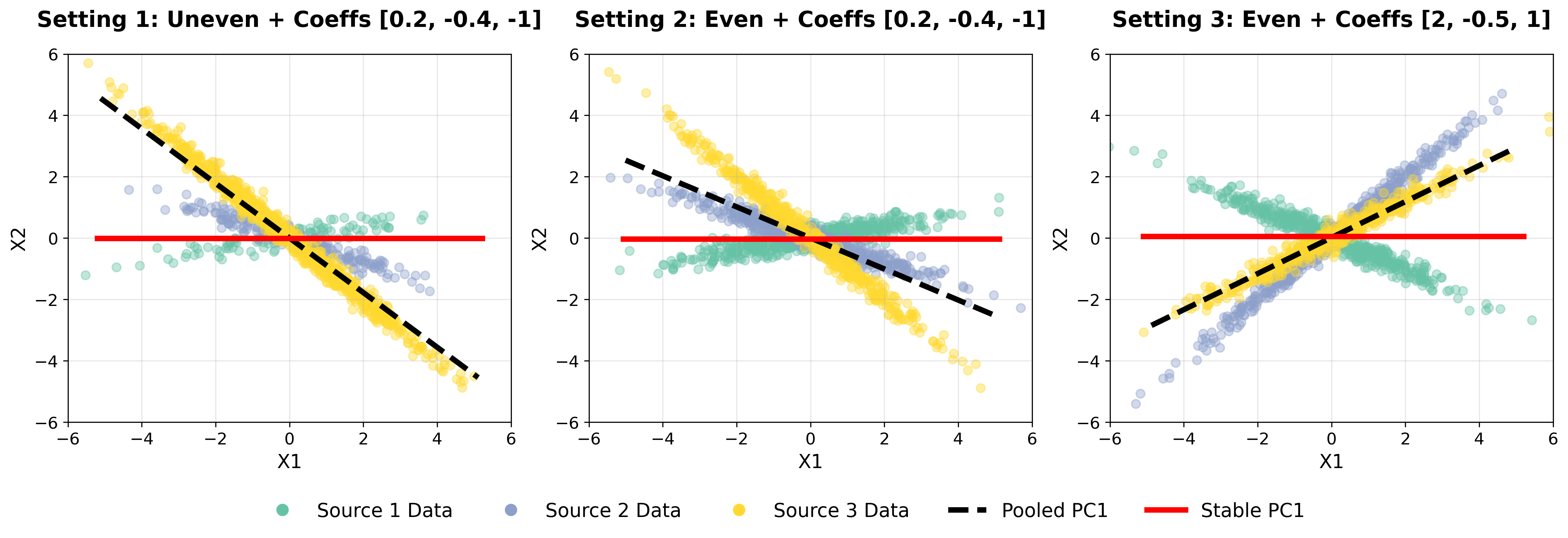
Figure 1: Comparison of the first principal component estimated by PooledPCA (dashed black) and StablePCA (solid red) across settings 1, 2, and 3. PooledPCA directions vary with the sample sizes and the source-specific relationships, while StablePCA consistently identifies the shared variation along $X_{1}$.

Figure 1 demonstrates the contrasting behavior of both methods. For PooledPCA, the estimated first principal component direction varies substantially across different settings, indicating that PooledPCA is highly sensitive to variations in sample sizes and source-specific coefficients $\beta$. In contrast, our proposed StablePCA, implemented using the later Algorithm 1 with $k=1$, consistently identifies the principal component along $X_{1}$ (the shared component), which removes the impact of imbalanced sample size (comparing Settings 1 and 2) and remains stable under heterogeneous structures in $X_{2}$ (comparing Settings 2 and 3).

3 Mirror Prox Algorithm for StablePCA

In Section 3.1, we provide detailed information on efficiently computing StablePCA in a data-dependent manner, along with a theoretical guarantee on convergence to the global optimal value in Section 3.2. For $1\leq l\leq L$, we observe $n_{l}$ i.i.d. samples $\{X^{(l)}_{i}\}_{i=1}^{n_{l}}$ drawn from the distribution $\mathbb{P}^{(l)}$. As a counterpart to the population version in (9), the empirical formulation of StablePCA is given by

$$\widehat{M}=\operatorname*{arg\,min}_{M\in\mathcal{F}^{k}}\max_{\omega\in\Delta^{L}}f(M,\omega),\quad\textrm{with}\quad f(M,\omega)=-\sum_{l=1}^{L}\omega_{l}\cdot\left\langle\widehat{\Sigma}^{(l)},M\right\rangle,$$ (13)

where $\widehat{\Sigma}^{(l)}=\frac{1}{n_{l}}\sum_{i=1}^{n_{l}}X^{(l)}_{i}[X^{(l)}_{i}]^{\intercal}$ is the empirical second-moment matrix for the $l$-th source.

3.1 Mirror Prox Algorithm with Optimistic Gradients

Even though it is a convex problem, (13) presents computation challenges due to its structured constraints: the matrix $M$ lies in the Fantope $\mathcal{F}^{k}$, while the weight vector $\omega$ belongs to the simplex $\Delta^{L}$. Standard gradient-based methods for minimax optimization, which alternate updates for $M$ and $\omega$, face two key issues here. First, projecting iterates onto the constraints $\mathcal{F}^{k}$ and $\Delta^{L}$ requires computationally intensive operations. Second, these methods exhibit suboptimal convergence rates in such structured constrained settings [6].

To address these challenges, we adopt the Mirror Prox algorithm, which is specifically designed for constrained optimization over non-Euclidean geometries. Unlike gradient descent ascent, Mirror Prox avoids explicit projections by leveraging a mirror map, which maps updates to the constraint set while respecting its geometry [5, 18]. This approach replaces Euclidean distances with Bregman divergences, a generalized measure of distance that adapts to the structure of $\mathcal{F}^{k}$ and $\Delta^{L}$. Consequently, mirror-based updates avoid expensive projections while achieving faster convergence.

Specifically, we introduce the following mirror maps tailored for the considered constraints: for $M\in\mathcal{F}^{k}$, and $\omega\in\Delta^{L}$,

$$\Phi_{1}(M)={\rm Tr}(M\log M),\quad\textrm{and}\quad\Phi_{2}(\omega)=\sum_{l=1}^{L}\omega_{l}\log\omega_{l}.$$

The associated Bregman divergences, which measure discrepancies between iterates belonging to $\mathcal{F}^{k}$ and $\Delta^{L}$, are given by:

$$\mathcal{D}_{\Phi_{1}}(M,M^{\prime})={\rm Tr}\left[M\left(\log M-\log M^{\prime}\right)\right],\quad\textrm{and}\quad\mathcal{D}_{\Phi_{2}}(\omega,\omega^{\prime})=\sum_{l=1}^{L}\omega_{l}\log\frac{\omega_{l}}{\omega^{\prime}_{l}},$$ (14)

for $M,M^{\prime}\in\mathcal{F}^{k}$, and $\omega,\omega^{\prime}\in\Delta^{L}$. For joint updates, we combine the above two divergences with weights $a,b>0$:

$$\mathcal{D}((M,\omega),(M^{\prime},\omega^{\prime}))=a\cdot\mathcal{D}_{\Phi_{1}}(M,M^{\prime})+b\cdot\mathcal{D}_{\Phi_{2}}(\omega,\omega^{\prime}),$$ (15)

where the weights $a,b$ will be specified in our following algorithm.

With the divergences defined in (15), we now describe the iterative Mirror Prox algorithm for solving the optimization problem (13). Since the minimax problem in (13) is convex-concave, convergence to the global optimum is guaranteed for any feasible initialization. We shall use the following starting values $(M^{0},\omega^{0})=(\bar{M}^{0},\bar{\omega}^{0})$ as the default starting values,

$$M^{0}=\bar{M}^{0}=\frac{k}{d}{\bf I}_{d}\in\mathcal{F}^{k},\quad\textrm{and}\quad\omega^{0}=\bar{\omega}^{0}=\frac{1}{L}\cdot{\bf 1}_{L}\in\Delta^{L}.$$ (16)

We now discuss how to update $M$ and $\omega$ at each iteration. In the $t$-th iteration with $t\geq 0$, the Mirror Prox algorithm performs two steps to compute the $(t+1)$-th update. It improves upon the standard mirror descent method by introducing an additional intermediate step, which provides a more accurate estimate of the future gradient direction. By incorporating this “look-ahead” information, Mirror Prox reduces oscillations near the saddle point and achieves a faster convergence rate. Specifically,

• At the first step, we compute an intermediate point $(\bar{M}^{t+1},\bar{\omega}^{t+1})$ using gradients evaluated at the previous intermediate point $(\bar{M}^{t},\bar{\omega}^{t})$. Given a prespecified step size $\eta>0$, the intermediate update is obtained by solving:

  $$(\bar{M}^{t+1},\bar{\omega}^{t+1})=\operatorname*{arg\,min}_{M\in\mathcal{F}^{k},\omega\in\Delta^{L}} \mathcal{D}((M,\omega),({M}^{t},{\omega}^{t}))$$ (17)

  $$\quad+\eta\cdot\left[\langle\nabla_{M}f(\bar{M}^{t},\bar{\omega}^{t}),M\rangle-\langle\nabla_{\omega}f(\bar{M}^{t},\bar{\omega}^{t}),\omega\rangle\right],$$

  where $D(\cdot,\cdot)$ denotes the Bregman divergence defined in (15).

• At the second step, we compute the next iterate $(M^{t+1},\omega^{t+1})$ using gradients evaluated at the new intermediate point $(\bar{M}^{t+1},\bar{\omega}^{t+1})$:

  $$(M^{t+1},\omega^{t+1})=\operatorname*{arg\,min}_{M\in\mathcal{F}^{k},\omega\in\Delta^{L}} \mathcal{D}((M,\omega),({M}^{t},{\omega}^{t}))$$ (18)

  $$+ \eta\cdot\left[\langle\nabla_{M}f(\bar{M}^{t+1},\bar{\omega}^{t+1}),M\rangle-\langle\nabla_{\omega}f(\bar{M}^{t+1},\bar{\omega}^{t+1}),\omega\rangle\right].$$

Note that during the whole procedure, the gradients are always evaluated using the intermediate points $\{(\bar{M}^{t},\bar{\omega}^{t})\}_{t}$ as shown in (17) and (18), while the Bregman divergences are evaluated with respect to $\{({M}^{t},{\omega}^{t})\}_{t}$.

We now present the intuition behind the first-step update in (17); a similar idea applies to the second-step update in (18). To motivate the formulation, consider a standard unconstrained optimization problem $\min_{x\in\mathbb{R}^{d}}g(x)$, where $g(\cdot)$ is convex and differentiable. The classical gradient descent update with a step size $\eta$ is:

$$x^{t+1}=x^{t}-\eta\nabla g(x^{t})=\operatorname*{arg\,min}_{x}\left\{\eta\langle\nabla g(x^{t}),x\rangle+\frac{1}{2}\|x-x^{t}\|_{2}^{2}\right\},$$

which can be interpreted as a trade-off between moving in the descent direction and staying close to the previous iterate. Mirror descent generalizes this by replacing the squared Euclidean distance with a Bregman divergence, enabling the adaptation to the underlying geometry of the constraint set. In our case, we minimize over $M\in\mathcal{F}^{k}$ and maximize over $\omega\in\Delta^{L}$. Thus, given the current point $(M^{t},\omega^{t})$ and gradients evaluated at the intermediate point $(\bar{M}^{t},\bar{\omega}^{t})$, we update the intermediate iterates $(\bar{M}^{t+1},\bar{\omega}^{t+1})$ via:

$$\bar{M}^{t+1}=\operatorname*{arg\,min}_{M\in\mathcal{F}^{k}}\left\{\frac{\eta}{a}\cdot\langle\nabla_{M}f(\bar{M}^{t},\bar{\omega}^{t}),M\rangle+D_{\Phi_{1}}(M,M^{t})\right\},$$

and

$$\bar{\omega}^{t+1}=\operatorname*{arg\,min}_{\omega\in\Delta^{L}}\left\{-\frac{\eta}{b}\cdot\langle\nabla_{\omega}f(\bar{M}^{t},\bar{\omega}^{t}),\omega\rangle+D_{\Phi_{2}}(\omega,\omega^{t})\right\},$$

where $D_{\Phi_{1}},D_{\Phi_{2}}$ are the Bregman divergences defined in 14, and the scaling factors $\eta/a,\eta/b$ adjust the step size according to the geometry of the constraints. By combining these two updates into a joint optimization and using the joint Bregman divergence defined in (15), we recover the first-step update in (17).

The following proposition provides the explicit form of the solutions to the steps in (17) and (18), enabling efficient updates.

Proposition 1

$(\bar{M}^{t+1},\bar{\omega}^{t+1})$ in (17) admits the following expression:

$$\bar{\omega}^{t+1}_{l}=\frac{{\omega}^{t}_{l}\exp\left(-\frac{\eta}{b}\langle\widehat{\Sigma}^{(l)},\bar{M}^{t}\rangle\right)}{\sum_{l=1}^{L}{\omega}^{t}_{l}\exp\left(-\frac{\eta}{b}\langle\widehat{\Sigma}^{(l)},\bar{M}^{t}\rangle\right)},\quad\bar{M}^{t}=\sum_{j=1}^{d}\min\left\{\exp\left(\bar{\lambda}^{t}_{j}+\bar{\nu}^{t}\right),1\right\}\bar{U}_{j}^{t}[\bar{U}_{j}^{t}]^{\intercal},$$ (19)

where $\bar{\lambda}^{t}\in\mathbb{R}^{d},\bar{U}^{t}\in\mathbb{R}^{d\times d}$ are the eigenvalues and eigenvectors of $\frac{\eta}{a}\sum_{l=1}^{L}\bar{\omega}_{l}^{t}\widehat{\Sigma}^{(l)}+\log M^{t}$, and $\bar{\nu}^{t}$ is the solution to $\sum_{j=1}^{d}\min\left\{\exp(\bar{\lambda}_{j}^{t}+\nu),1\right\}=k$. Similarly, $(M^{t+1},\omega^{t+1})$ in (18) admits the following expression:

$${\omega}^{t+1}_{l}=\frac{{\omega}^{t}_{l}\exp\left(-\frac{\eta}{b}\langle\widehat{\Sigma}^{(l)},\bar{M}^{t+1}\rangle\right)}{\sum_{l=1}^{L}{\omega}^{t}_{l}\exp\left(-\frac{\eta}{b}\langle\widehat{\Sigma}^{(l)},\bar{M}^{t+1}\rangle\right)},\quad{M}^{t+1}=\sum_{j=1}^{d}\min\left\{\exp\left(\bar{\lambda}^{t+1}_{j}+\bar{\nu}^{t+1}\right),1\right\}\bar{U}_{j}^{t+1}[\bar{U}_{j}^{t+1}]^{\intercal},$$ (20)

where $\bar{\lambda}^{t+1}\in\mathbb{R}^{d},\bar{U}^{t+1}\in\mathbb{R}^{d\times d}$ are the eigenvalues and eigenvectors of $\frac{\eta}{a}\sum_{l=1}^{L}\bar{\omega}_{l}^{t+1}\widehat{\Sigma}^{(l)}+\log M^{t}$, and $\bar{\nu}^{t+1}$ is the solution to $\sum_{j=1}^{d}\min\left\{\exp(\bar{\lambda}_{j}^{t+1}+\nu),1\right\}=k$.

Upon completing $T$ iterations of the Mirror Prox algorithm, we collect the averaged iterates $\frac{1}{T}\sum_{t=1}^{T}\bar{M}^{t}$ as $\widehat{M}$, the solution to the relaxed problem over the Fantope $\mathcal{F}^{k}$, defined in (13). Recall that the goal of the original nonconvex multi-source PCA is to solve:

$$\min_{M\in\mathcal{P}^{k}}\max_{\omega\in\Delta^{L}}f(M,\omega),$$ (21)

where $\mathcal{P}^{k}$ denotes the set of rank-$k$ projection matrices as defined in (1). Since the relaxed solution $\widehat{M}$ may not have exact rank $k$, we perform a final projection onto $\mathcal{P}^{k}$ to enforce the rank constraint. Specifically, let $\{U_{i}\}_{i=1}^{k}$ denote the top $k$ eigenvectors of $\widehat{M}$, then the projected solution is given by:

$$\widehat{M}^{\rm Proj}=\sum_{i=1}^{k}U_{i}U_{i}^{\intercal}.$$ (22)

In Section 3.2, we further discuss when the projected $\widehat{M}^{\rm Proj}$ nearly solves the original nonconvex optimization problem in (21).

The procedure of solving StablePCA is provided in Algorithm 1.

Data: Estimated $\{\widehat{\Sigma}^{(l)}\}_{l\in[L]}$; hyperparameters for Mirror Prox: $\eta$, $a$, $b$; maximum iteration $T$; tolerance $\epsilon$

Set initial values $(M^{0},\omega^{0}),(\bar{M}^{0},\bar{\omega}^{0})$ as in (16), and ${\rm gap}=1$,

while $t=1,...,T$ and ${\rm gap}>\epsilon$ do

    Update $(\bar{M}^{t+1},\bar{\omega}^{t+1})$ as shown in (19);

   Update $(M^{t+1},\omega^{t+1})$ as shown in (20);

   Set $\widehat{M}=\frac{1}{t}\sum_{s=1}^{t}\bar{M}^{s}$ and $\widehat{\omega}=\frac{1}{t}\sum_{s=1}^{t}\bar{\omega}^{s}$.

   Calculate the duality gap: ${\rm gap}=\max_{\omega\in\Delta^{L}}f(\widehat{M},\omega)-\min_{M\in\mathcal{F}^{k}}f(M,\widehat{\omega})$.

end while

Return $\widehat{M},\widehat{\omega}$ and the projected rank-$k$ $\widehat{M}^{\rm Proj}$ as in (22).

Algorithm 1 Mirror Prox Algorithm for StablePCA

We provide the implementation details on the hyperparameter selections for Algorithm 1. Following [6], we set the mirror map parameters as $a=\frac{1}{k\log d}$ and $b=\frac{1}{\log L}$, which correspond to the inverse logarithmic measures of the constraint sets $\mathcal{F}^{K}$ and $\Delta^{L}$. While a constant learning rate $\eta$ guarantees convergence, as shown in the following Theorem 2, our empirical implementation employs the adaptive learning rate scheme from [4]. This adaptation to the objective’s local smoothness, while maintaining communication between the primal and dual variables, leads to accelerated convergence in practice.

3.2 Theoretical Justification for Global Convergence

We establish the convergence of Algorithm 1 in the following theorem.

Theorem 2

With the specified hyperparameters $a=\frac{1}{k\log d}$, $b=\frac{1}{\log L}$, and learning rate

$$\eta=(8\cdot\sqrt{(k\log d)\cdot(\log L)}\cdot\max_{1\leq l\leq L}\|\widehat{\Sigma}^{(l)}\|_{\rm op})^{-1},$$

the outputs $\widehat{M}$ and $\widehat{\omega}$ from Algorithm 1 achieve the following convergence rate:

$$0\leq\max_{\omega\in\Delta^{L}}f(\widehat{M},\omega)-\min_{M\in\mathcal{F}^{k}}f(M,\widehat{\omega})\leq\frac{16\cdot\sqrt{(k\log d)\cdot(\log L)}\cdot\max_{1\leq l\leq L}\|\widehat{\Sigma}^{(l)}\|_{\rm op}}{T},$$

where $\widehat{M},\widehat{\omega}$ are the averaged iterates, defined as $\widehat{M}=\frac{1}{T}\sum_{t=1}^{T}\bar{M}^{t}$ and $\widehat{\omega}=\frac{1}{T}\sum_{t=1}^{T}\bar{\omega}^{t}$.

We now discuss the implications of the above theorem. By Sion’s Minimax Theorem [26, 15], we have the decomposition

$$\max_{\omega\in\Delta^{L}}f(\widehat{M},\omega)-\min_{M\in\mathcal{F}^{k}}f(M,\widehat{\omega})= \left[\max_{\omega\in\Delta^{L}}f(\widehat{M},\omega)\right]-\min_{M\in\mathcal{F}^{k}}\left[\max_{\omega\in\Delta^{L}}f(M,\omega)\right]$$

$$+\max_{\omega\in\Delta^{L}}\left[\min_{M\in\mathcal{F}^{k}}f(M,\omega)\right]-\left[\min_{M\in\mathcal{F}^{k}}f(M,\widehat{\omega})\right]\geq 0.$$

Combining this decomposition with Theorem 2, we obtain that there exists a positive constant $C>0$ such that

$$0\leq\max_{\omega\in\Delta^{L}}f(\widehat{M},\omega)-\min_{M\in\mathcal{F}^{k}}\left[\max_{\omega\in\Delta^{L}}f(M,\omega)\right]\leq C/T,$$ (23)

showing that $\widehat{M}$ achieves the global minimum of $\min_{M\in\mathcal{F}^{k}}[\max_{\omega\in\Delta^{L}}f(M,\omega)]$ with an error of order $\mathcal{O}(T^{-1})$.

We now study how well the rank-$k$ matrix $\widehat{M}^{\rm Proj}$, obtained by projecting $\widehat{M}$ onto $\mathcal{P}^{k}$, approximates the solution to the original nonconvex minimax problem (21).

Theorem 3

Under the same conditions of Theorem 2, the output $\widehat{M}^{\rm Proj}$ from Algorithm 1 satisfies:

$$0\leq\max_{\omega\in\Delta^{L}}f(\widehat{M}^{\rm Proj},\omega)-\min_{M\in\mathcal{P}^{k}}\left[\max_{\omega\in\Delta^{L}}f(M,\omega)\right]\leq\tau(\widehat{M}^{\rm Proj},\widehat{M})+C/T,$$

where $C>0$ is a constant independent of $T$ and $\tau(\widehat{M}^{\rm Proj},\widehat{M})$ quantifies the optimality gap induced by the final projection step, defined as:

$$\tau(\widehat{M}^{\rm Proj},\widehat{M})\coloneqq\max_{\omega\in\Delta^{L}}f(\widehat{M}^{\rm Proj},\omega)-\max_{\omega\in\Delta^{L}}f(\widehat{M},\omega).$$ (24)

In practice, given the outputs $\widehat{M}^{\rm Proj},\widehat{M}$ from Algorithm 1, we can compute the optimality gap $\tau(\widehat{M}^{\rm Proj},\widehat{M})$ and verify whether $\tau(\widehat{M}^{\rm Proj},\widehat{M})\leq\frac{\epsilon}{2}$, for a small tolerance $\epsilon>0$. Then as long as $T\gtrsim 1/\epsilon$, the projected estimator $\widehat{M}^{\rm Proj}$ is an $\epsilon$-optimal solution to the original nonconvex minimax optimization problem in (21), satisfying:

$$\max_{\omega\in\Delta^{L}}f(\widehat{M}^{\rm Proj},\omega)-\min_{M\in\mathcal{P}^{k}}\left[\max_{\omega\in\Delta^{L}}f(M,\omega)\right]\leq\epsilon.$$

As shown in Figure 4 of Section 4.2, the gap $\tau(\widehat{M}^{\rm Proj},\widehat{M})$ is empirically negligible in our simulated experiments. This suggests that in practice, the relaxed solution followed by the spectral projection provides a near-optimal approximation to the original nonconvex multi-source PCA in (21).

4 Simulations

4.1 Worst-case Explained Variance

We consider the setting with $L=4$ independent data sources, each comprising $n=500$ observations $X^{(l)}_{i}\in\mathbb{R}^{d}$, for $i=1,...,n$, and $l=1,...L$. The data generation mechanism is as follows. First, we generate matrices $W_{\rm share}\in\mathbb{R}^{d\times 5}$ and $W_{\rm source}^{(l)}\in\mathbb{R}^{d\times(d/2-5)}$, for each $l=1,...,L$, where each entry is independently drawn from $\mathcal{N}(0,1)$. Here, $W_{\rm share}$ represents a low-rank structure shared across all sources, while $W_{\rm source}^{(l)}$ introduces source-specific variations. Then for each source $l$ and each sample $i$, we generate data according to:

$$X^{(l)}_{i}=\frac{1}{\sqrt{d}}\left((W_{\rm share},W_{\rm source}^{(l)})Z^{(l)}_{i}+\epsilon_{i}^{(l)}\right),\quad\textrm{with $Z^{(l)}_{i}\sim\mathcal{N}(0_{d/2},{\bf I}_{d/2})$}$$ (25)

where $\epsilon^{(l)}_{i}\sim\mathcal{N}(0_{d},0.25{\bf I}_{d})$. The scaling factor $d^{-1/2}$ ensures consistent signal magnitude across varied dimensions $d\in[20,30,...,100]$.

We compare the proposed StablePCA method against the PooledPCA approach, which applies standard PCA to pooled data across all sources. The comparison focuses on the worst-case explained variance, evaluated both in-distribution and out-of-distribution:

• In-distribution worst-case explained variance. The explained variance is computed separately for each of the $L=4$ sources, and we report the minimum across sources:

  $$\min_{1\leq l\leq L}\frac{1}{n}\sum_{i=1}^{n}\left((X^{(l)}_{i})^{2}-(X^{(l)}_{i}-\widehat{X}^{(l)}_{i})^{2}\right),$$

  where $\widehat{X}^{(l)}_{i}$ denotes the projection of $X^{(l)}_{i}$ from each method, both implemented with rank $k=5$. This is an out-of-sample result, that method is evaluated on independent samples regenerated according to (25).

• Out-of-distribution worst-case explained variance. We generate $L_{\rm out}=100$ new test distributions. For each $l^{\prime}=1,...,L_{\rm out}$, we generate samples according to the same mechanisms as in (25), using the shared $W_{\rm share}$, but independently sampling new $W^{(l^{\prime})}_{\rm source}$. In addition, we shift and rescale the latent factors via $Z^{(l^{\prime})}_{i}\sim\mathcal{N}(\alpha^{(l^{\prime})},\sigma^{(l^{\prime})}\cdot{\bf I}_{d/2})$, where $\alpha^{(l^{\prime})}$ and $\sigma^{(l^{\prime})}$ are drawn uniformly from $\{-1,0,1\}$ and $\{0.5,1,1.5,2\}$, respectively. The out-of-distribution worst-case explained variance is then defined on these new test distributions:

  $$\min_{1\leq l^{\prime}\leq L_{\rm out}}\frac{1}{n}\sum_{i=1}^{n}\left((X^{(l^{\prime})}_{i})^{2}-(X^{(l^{\prime})}_{i}-\widehat{X}^{(l^{\prime})}_{i})^{2}\right).$$

Figure 2 presents two key findings: (1) StablePCA demonstrates uniformly better worst-case performance than PooledPCA across all dimensions considered, for both in-distribution and out-of-distribution evaluations (the leftmost and the middle panels), and (2) its computational time scales moderately with dimension while maintaining practical feasibility (the rightmost panel). These results are summarized over 100 independent simulation trials.

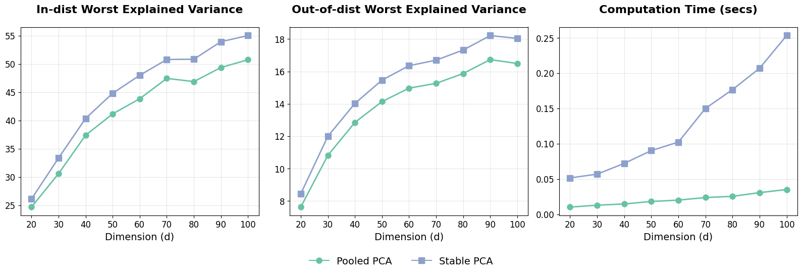
Figure 2: Comparative performance of StablePCA (blue squares) and PooledPCA (green circles) with dimensions $d\in\{20,30,...,100\}$. Leftmost: In-distribution worst-case explained variance. Middle: Out-of-distribution worst-case explained variance. Rightmost: Computation time (seconds) versus dimension.

4.2 Finite-sample error and cost of low rank projection

In this experiment, we first assess the finite-sample error of the empirical StablePCA estimator in (9) compared to the population-level solution in (13). We then assess the information loss incurred by the low rank approximation (the last step in Algorithm 3), by projecting empirical StablePCA onto a rank-$k$ subspace.

The data generation mechanism follows (25), with sample sizes $n\in\{500,1000,...,5000\}$ and $d\in\{10,20,30\}$. In Figure 3, we report the distance between the empirical estimator $\widehat{M}$, obtained via Algorithm 1 (without applying the final spectral truncation), and the population-level solution $M^{*}$, computed with $n=200,000$ samples using Algorithm 1. The distance is measured by $\|\widehat{M}-M^{*}\|_{\rm op}$. The results show that the estimation error systematically decreases as the sample size increases across all dimensions considered.

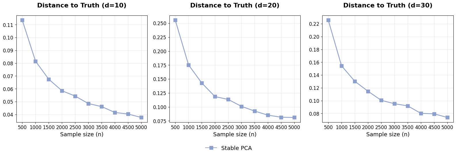
Figure 3: Finite-sample error $\|\widehat{M}-M^{*}\|_{\rm op}$ across samples sizes $n\in\{500,1000,...,5000\}$ and $d\in\{10,20,30\}$. $\widehat{M}$ is the empirical StablePCA implemented by Algorithm 1 without applying the final spectral truncation. $M^{*}$ represents the population-level StablePCA, computed with $n=200,000$ samples using Algorithm 1.

Next, in Figure 4, we investigate the optimality gap $\tau(\widehat{M}^{\rm Proj},\widehat{M})$ defined in (24), where $\widehat{M}^{\rm Proj},\widehat{M}$ are the outputs of Algorithm 1 with and without the last projection step, respectively. The results show that for all $d\in\{10,20,30\}$, the optimality gap remains small, with values in the range of $[0.007,0.02]$, across all sample sizes $n$ considered. As implied in Theorem 24, this numerical result indicates that $\widehat{M}^{\rm Proj}$ nearly solves the original nonconvex multi-source PCA in (21).

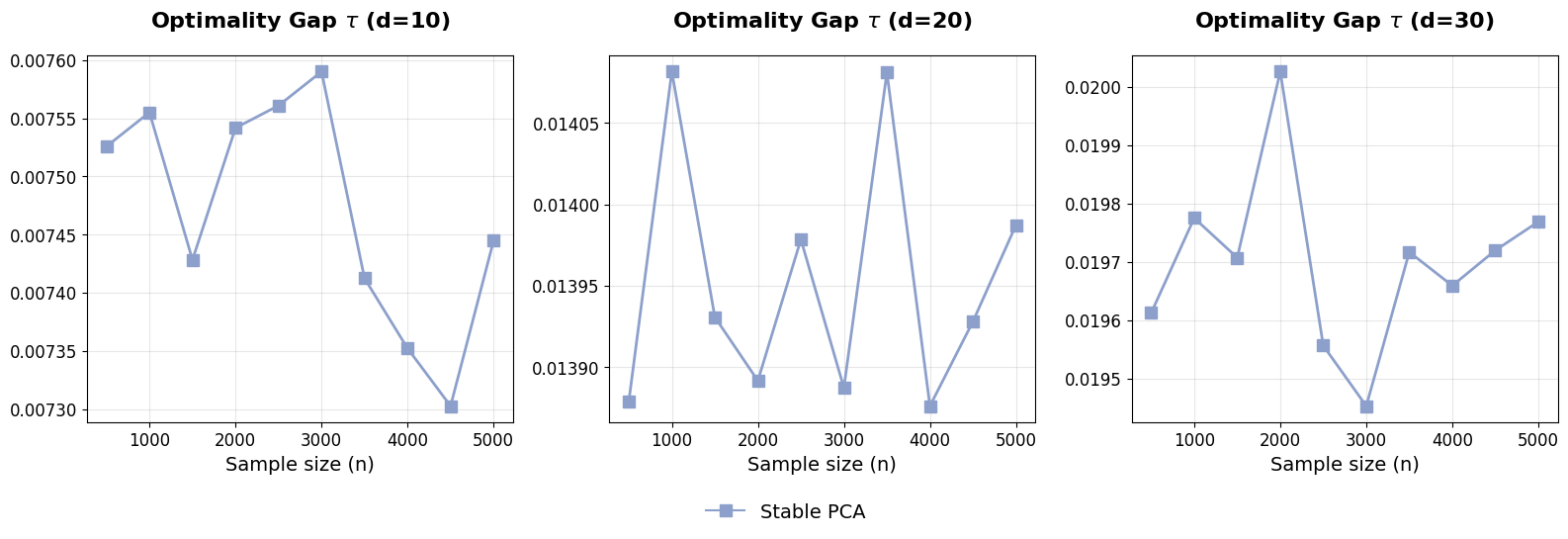
Figure 4: The optimality gap $\tau(\widehat{M}^{\rm Proj},\widehat{M})\coloneqq\max_{\omega\in\Delta^{L}}f(\widehat{M}^{\rm Proj},\omega)-\max_{\omega\in\Delta^{L}}f(\widehat{M},\omega)$, across sample sizes $n\in\{500,1000,1500,...,5000\}$ and $d\in\{10,20,30\}$. $\widehat{M}^{\rm Proj},\widehat{M}$ are the outputs of Algorithm 1 with and without the last projection step, respectively.

5 Conclusions and Discussions

In this work, we propose StablePCA, a distributionally robust framework for learning shared principal directions across multiple sources while accounting for potential distributional shifts in future populations. To address the nonconvexity inherent in the original formulation, we reformulate the problem as a convex optimization by employing a Fantope relaxation of the rank constraint. Moreover, we develop a Mirror Prox algorithm with explicit closed-form updates at each iteration, ensuring that the optimization procedure remains computationally efficient. Lastly, we provide a strategy to evaluate whether the projected output nearly solves the original nonconvex formulation.

Our key insights of handling distributionally robust PCA may be extended to other problems of studying the shared representation shared across multiple domains. As an example, our developed method can be extended to address stable Canonical Correlation Analysis (CCA) [9]. In specific, suppose there are two sets of high-dimensional features $X\in\mathbb{R}^{d}$ and $Y\in\mathbb{R}^{m}$ and we are interested in solving the group distributionally robust CCA problem for $Q^{*}_{\rm d-CCA}=U^{*}(V^{*})^{\intercal}$, where

$$U^{*},V^{*}=\operatorname*{arg\,min}_{U\in\mathbb{R}^{d\times k},V\in\mathbb{R}^{m\times k}}\max_{l\in[L]}~{\rm Tr}\left(U^{\intercal}C_{XY}^{(l)}V\right),\quad{\rm s.t.}\quad U^{\intercal}U=V^{\intercal}V={\bf I}_{k}$$ (26)

where $C_{XY}^{(l)}=\{{\Sigma}^{(l)}_{X}\}^{-1/2}{\Sigma}^{(l)}_{XY}\{{\Sigma}^{(l)}_{Y}\}^{-1/2}$, ${\Sigma}^{(l)}_{X}$, ${\Sigma}^{(l)}_{Y}$, and ${\Sigma}^{(l)}_{XY}$ represent source $l$’s population-level covariance matrices of $X$, $Y$ and that between $X$ and $Y$ respectively, $k\ll d,m$, and $Q^{*}_{\rm d-CCA}\in\mathbb{R}^{d\times m}$ is a low-rank matrix analog to $M^{*}_{\rm d-PCA}$ defined in the original multi-source PCA problem (6). Similar to (6), this stable CCA problem also encounters the nonconvexity issue due to the rank constraints. Inspired by the convex relaxation for CCA [8], one could relax (26) by introducing the convex constraint set

$$\mathcal{F}^{k}_{\rm CCA}=\left\{Q\in\mathbb{R}^{d\times m}:\|Q\|_{\rm op}\leq 1,\|Q\|_{*}\leq k\right\},$$

where $\|\cdot\|_{*}$ represents the nuclear norm that $\|A\|_{*}={\rm Tr}(\{A^{\intercal}A\}^{1/2})$. Then he corresponding relaxed minimax problem becomes:

$$Q^{*}=\operatorname*{arg\,min}_{Q\in\mathcal{F}^{k}_{\rm CCA}}\max_{\omega\in\Delta_{L}}~-\sum_{l=1}^{L}\omega_{l}\left\langle C_{XY}^{(l)},Q\right\rangle,$$ (27)

as an extension of the fantope-relaxed version of StablePCA defined in (9). The relaxed problem (27) is convex-concave and can be efficiently solved by extending the optimistic-gradient Mirror Prox algorithm presented in Section 3. This extension requires substituting the mirror map used for $\mathcal{F}^{k}$ in StablePCA with one tailored to $\mathcal{F}^{k}_{\rm CCA}$.

References

- [1] Pranjal Awasthi, Satyen Kale, and Ankit Pensia. Semi-supervised group dro: Combating sparsity with unlabeled data. In International Conference on Algorithmic Learning Theory, pages 125–160. PMLR, 2024.
- [2] Prabhu Babu and Petre Stoica. Fair principal component analysis (pca): minorization-maximization algorithms for fair pca, fair robust pca and fair sparse pca. arXiv preprint arXiv:2305.05963, 2023.
- [3] Francis Bach. Learning theory from first principles. MIT press, 2024.
- [4] Francis Bach and Kfir Y Levy. A universal algorithm for variational inequalities adaptive to smoothness and noise. In Conference on learning theory, pages 164–194. PMLR, 2019.
- [5] Amir Beck and Marc Teboulle. Mirror descent and nonlinear projected subgradient methods for convex optimization. Operations Research Letters, 31(3):167–175, 2003.
- [6] Sébastien Bubeck et al. Convex optimization: Algorithms and complexity. Foundations and Trends® in Machine Learning, 8(3-4):231–357, 2015.
- [7] Jon Dattorro. Convex optimization & Euclidean distance geometry. Lulu. com, 2010.
- [8] Chao Gao, Zongming Ma, and Harrison H Zhou. An efficient and optimal method for sparse canonical correlation analysis. ArXiV e-prints, 1409, 2014.
- [9] Chao Gao, Zongming Ma, and Harrison H Zhou. Sparse cca: Adaptive estimation and computational barriers. 2017.
- [10] Zijian Guo. Statistical inference for maximin effects: Identifying stable associations across multiple studies. Journal of the American Statistical Association, pages 1–17, 2023.
- [11] Surya Narayanan Hari, Eliezer Van Allen, Jackson Nyman, Nicita Mehta, Bowen Jiang, Haitham Elmarakeby, Felix Dietlein, Jacob Rosenthal, Eshna Sengupta, Renato Umeton, et al. Using distributionally robust optimization to improve robustness in cancer pathology. In NeurIPS 2021 Workshop on Distribution Shifts: Connecting Methods and Applications.
- [12] Chuan Hong, Everett Rush, Molei Liu, Doudou Zhou, Jiehuan Sun, Aaron Sonabend, Victor M Castro, Petra Schubert, Vidul A Panickan, Tianrun Cai, et al. Clinical knowledge extraction via sparse embedding regression (keser) with multi-center large scale electronic health record data. NPJ digital medicine, 4(1):1–11, 2021.
- [13] Weihua Hu, Gang Niu, Issei Sato, and Masashi Sugiyama. Does distributionally robust supervised learning give robust classifiers? In International Conference on Machine Learning, pages 2029–2037. PMLR, 2018.
- [14] Mohammad Mahdi Kamani, Farzin Haddadpour, Rana Forsati, and Mehrdad Mahdavi. Efficient fair principal component analysis. Machine Learning, pages 1–32, 2022.
- [15] Hidetoshi Komiya. Elementary proof for sion’s minimax theorem. Kodai mathematical journal, 11(1):5–7, 1988.
- [16] Mengyan Li, Xiaoou Li, Kevin Pan, Alon Geva, Doris Yang, Sara Morini Sweet, Clara-Lea Bonzel, Vidul Ayakulangara Panickan, Xin Xiong, Kenneth Mandl, et al. Multisource representation learning for pediatric knowledge extraction from electronic health records. NPJ Digital Medicine, 7(1):319, 2024.
- [17] Nicolai Meinshausen and Peter Bühlmann. Maximin effects in inhomogeneous large-scale data. The Annals of Statistics, 43(4):1801–1830, 2015.
- [18] Arkadi Nemirovski. Prox-method with rate of convergence o (1/t) for variational inequalities with lipschitz continuous monotone operators and smooth convex-concave saddle point problems. SIAM Journal on Optimization, 15(1):229–251, 2004.
- [19] Matt Olfat and Anil Aswani. Convex formulations for fair principal component analysis. In Proceedings of the AAAI Conference on Artificial Intelligence, volume 33, pages 663–670, 2019.
- [20] Michael L Overton and Robert S Womersley. On the sum of the largest eigenvalues of a symmetric matrix. SIAM Journal on Matrix Analysis and Applications, 13(1):41–45, 1992.
- [21] Vidhi Rathore and Naresh Manwani. Achieving fair pca using joint eigenvalue decomposition. arXiv preprint arXiv:2502.16933, 2025.
- [22] Benjamin Recht, Maryam Fazel, and Pablo A Parrilo. Guaranteed minimum-rank solutions of linear matrix equations via nuclear norm minimization. SIAM review, 52(3):471–501, 2010.
- [23] Shiori Sagawa, Pang Wei Koh, Tatsunori B Hashimoto, and Percy Liang. Distributionally robust neural networks for group shifts: On the importance of regularization for worst-case generalization. arXiv preprint arXiv:1911.08731, 2019.
- [24] Samira Samadi, Uthaipon Tantipongpipat, Jamie H Morgenstern, Mohit Singh, and Santosh Vempala. The price of fair pca: One extra dimension. Advances in neural information processing systems, 31, 2018.
- [25] Junhui Shen, Aaron J Davis, Ding Lu, and Zhaojun Bai. Hidden convexity of fair pca and fast solver via eigenvalue optimization. arXiv preprint arXiv:2503.00299, 2025.
- [26] Maurice Sion. On general minimax theorems. 1958.
- [27] Hoa Thi Nhu Tran, Kok Siong Ang, Marion Chevrier, Xiaomeng Zhang, Nicole Yee Shin Lee, Michelle Goh, and Jinmiao Chen. A benchmark of batch-effect correction methods for single-cell rna sequencing data. Genome biology, 21:1–32, 2020.
- [28] Vincent Q Vu, Juhee Cho, Jing Lei, and Karl Rohe. Fantope projection and selection: A near-optimal convex relaxation of sparse pca. Advances in neural information processing systems, 26, 2013.
- [29] Zhenyu Wang, Peter Bühlmann, and Zijian Guo. Distributionally robust machine learning with multi-source data, 2023.
- [30] Zitao Wang, Nian Si, Zijian Guo, and Molei Liu. Multi-source stable variable importance measure via adversarial machine learning. arXiv preprint arXiv:2409.07380, 2024.
- [31] Jingzhao Zhang, Aditya Menon, Andreas Veit, Srinadh Bhojanapalli, Sanjiv Kumar, and Suvrit Sra. Coping with label shift via distributionally robust optimisation. arXiv preprint arXiv:2010.12230, 2020.
- [32] Zihan Zhang, Wenhao Zhan, Yuxin Chen, Simon S Du, and Jason D Lee. Optimal multi-distribution learning. In The Thirty Seventh Annual Conference on Learning Theory, pages 5220–5223. PMLR, 2024.