Dynamic and Distributed Routing in IoT Networks based on Multi-Objective Q-Learning

Abstract

The last few decades have witnessed a rapid increase in IoT devices owing to their wide range of applications, such as smart healthcare monitoring systems, smart cities, and environmental monitoring. A critical task in IoT networks is sensing and transmitting information over the network. The IoT nodes gather data by sensing the environment and then transmit this data to a destination node via multi-hop communication, following some routing protocols. These protocols are usually designed to optimize possibly contradictory objectives, such as maximizing packet delivery ratio and energy efficiency. While most literature has focused on optimizing a static objective that remains unchanged, many real-world IoT applications require adapting to rapidly shifting priorities. For example, in monitoring systems, some transmissions are time-critical and require a high priority on low latency, while other transmissions are less urgent and instead prioritize energy efficiency. To meet such dynamic demands, we propose novel dynamic and distributed routing based on multiobjective Q-learning that can adapt to changes in preferences in real-time. Our algorithm builds on ideas from both multi-objective optimization and Q-learning. We also propose a novel greedy interpolation policy scheme to take near-optimal decisions for unexpected preference changes. The proposed scheme can approximate and utilize the Pareto-efficient solutions for dynamic preferences, thus utilizing past knowledge to adapt to unpredictable preferences quickly during runtime. Simulation results show that the proposed scheme outperforms state-of-the-art algorithms for various exploration strategies, preference variation patterns, and important metrics like overall reward, energy efficiency, and packet delivery ratio.

I Introduction

In recent years, rapid growth has been witnessed in Machine-to-Machine (M2M) communications and IoT networks owing to their wide range of applications. A report by CISCO on IoT growth [1] made an estimated count of over 29.3 billion IoT devices as of 2023, up from 18.4 billion in 2018. In IoT-based networks, the intelligent IoT nodes continuously monitor the environment and send the data to some destination node(s) when events occur. The destination node could be a sink node gathering data, or a base station, or another IoT node that needs to process the data. Due to their limited power, these nodes do not send data directly to the destination node; rather, the packets are sent via various relay nodes following certain routing protocols. To facilitate smooth and efficient data communication to meet the increasing demands of future IoT networks, designing intelligent routing protocols is important.

When designing intelligent routing protocols for IoT networks, multiple objectives must be considered. Among important objectives are maximizing the PDR, minimizing energy consumption, minimizing delay, ensuring security, and maximizing throughput. Prioritizing one objective in routing may come at the cost of another objective. For example, the most energy-efficient path for delivering packets from a source to a destination node may not be the one promising maximum PDR, as it may involve more link failures, network congestion, or selective forwarding attacks. If the routing protocols select such paths to save energy, it might adversely affect other objectives, e.g, the PDR. When the objectives are conflicting, no one solution exists that co-optimizes all objectives. In such cases, reasonable trade-offs based on the user’s preferences can be found by using the tools of multi-objective optimization [2]. This is often done by scaling the objectives with weights reflecting user and network preferences. These weighted objectives can then be used to construct a Pareto front, representing the set of optimal solutions where no single objective can be improved without worsening another, thereby providing a comprehensive view of the trade-offs involved.

In many real-wold IoT applications the objective is not static over time, but can be changing. Consider, for example, monitoring networks where certain information is time-critical, while other data requires transmission but is less sensitive to latency. In such cases we might prioritize low-latency for the time-sensitive transmissions, placing significant weight on the latency objective. Conversely, for less time-sensitive transmissions, we could prioritize other objectives, such as energy efficiency or security. As another example, consider a network with fluctuating energy supply. At certain times, when the energy are constrained, or nodes are running out of battery, there might be a need to prioritize energy conservation in the network, even if we may have to give lesser preference to other objectives. When energy is not scarce then we might prioritize other objectives. Such networks necessitate algorithms that can dynamically adjust to shifting objectives in real-time, ensuring optimal performance across varying conditions.

Future IoT networks will necessitate a new generation of distributed algorithms that are resource-aware and can optimize multiple objectives dynamically, adapting to the changing network preferences in real-time. Reinforcement Learning (RL) offers a promising solution to these problems owing to its ability to make intelligent responses to the environment based on experience of interacting with the environment. However, existing research (discussed in Section II) does not address dynamic objectives. Even studies considering multiple objectives typically scale these objectives without allowing for changes over time. The key contribution of this paper is to provide novel distributed algorithms that can learn to deal with multiple dynamic objective preferences in real-time.

In particular, our main contributions are:

1. We propose a novel dynamic preference Q-Learning routing algorithm that learns optimal decisions for multiple preferences in real-time. The algorithm adapts online to changing preferences, allowing it to continuously adjust to new objectives and conditions.

2. The proposed algorithm can be implemented in a distributed manner, with each node learning a local Q-table based on its actions, communicating only with neighbors in the routing network, and requiring no central information during training.

3. Extensive simulations compare our dynamic preference Q-Learning algorithm to six baseline schemes. We illustrate its performance using different exploration strategies, showing significant improvements in adaptability and routing efficiency over the baseline algorithms.

The paper is organized as follows: Section II discusses related work, Section III outlines the system model and problem formulation, Section IV details the proposed algorithm, Section V illustrates how the algorithm can be implemented in fully distributed manner, Section VI presents our simulation results, and Section VII concludes.

II Related Works

Over the last two decades, there has been an upsurge in research related to developing efficient routing protocols for wireless networks and IoT. Some works present enhancements in Dijkstra’s algorithm for routing [3, 4]. However, such routing protocols are often associated with high local computations, storage requirements, and time complexities. Thus, it is inefficient to utilize them for resource-contained IoT networks today since they have to deliver quality services to users. Also, some other heuristic-based methods like sleep scheduling [5], fuzzy logic [3], trust-based or cluster-based approaches such as MANET, and VANET [6, 7], are also unable to meet the multiobjective expectations from IoT of the present and future. With the evolution of Machine Learning (ML), many ML-based approaches have been presented as promising solutions to routing-related optimization problems. Some of these routing algorithms are built on ML paradigms such as clustering [6], and evolutionary algorithms [8].

RL, among other data-driven ML approaches, has attracted special attention since it provides us with the facility to learn optimal policies while interacting with the environment. Thus, many RL-based routing protocols have been proposed [9, 10, 11, 12, 13, 14, 15, 16, 17, 18, 19, 20, 21, 22, 23, 24, 25, 26, 27, 28, 29]. A direct utilization of RL for IoT is to rely upon a central controller for route planning and control. This has been made possible by the recent development of software-defined networking (SDN). In SDN-enabled IoT networks, a central controller has complete knowledge of the network topology and takes most of the control decisions in the network. The SDN-based centralized protocols face several challenges. Since the SDN controller plays a pivotal role in such protocols, it is an attractive target for malicious users to carry out DDoS attacks or other security attacks [30]. Such routing protocols are also vulnerable to single-point failures. Another critical issue in IoT networks is maintaining individual IoT nodes’ data privacy. Sharing all the data with a central controller can be both cost-inefficient and also pose a risk to data privacy. Moreover, as the size of IoT networks is increasing rapidly, scalability is a major issue with these centralized protocols [23].

With more intelligent organization, it is feasible and beneficial to employ distributed versions of RL algorithms for routing. As an example, in tabular Q-learning, SDN-based and other centralized approaches rely on a centralized controller to keep the knowledge of the entire network, store the entire Q-table, and do the whole route planning as the RL agent. However, the Q-table can be split into smaller parts, with each node having its local small Q-tables with information about and interaction with their immediate neighbors. In this way, each node acts as an RL agent capable of making its own decisions. Some existing research works utilize this possibility and thus propose distributed RL-based routing protocols [15, 14]. Abadi et al. [13] utilize a sleep scheduling mechanism for enhancing the energy efficiency of their RL-based routing protocol. Such sleep scheduling is difficult to achieve in a fully distributed setup. Thus, they utilize a semi-distributed approach. They divide the network into clusters, with each cluster head acting as the local controller for the cluster. In this work, however, we showcase how a fully distributed RL-based scheme can be effectively applied while ensuring high energy efficiency and other vital objectives.

While the RL-based routing protocols discussed so far work well for the static objective preference on which the model is trained, they cannot deal with changing preferences and objectives. However, in IoT networks, the user and network preferences keep changing in runtime. Existing RL-based approaches cannot quickly adapt to changes in the environment, and it takes time to relearn new policies suitable for new preferences. For example, Natarajan et al. [31] introduce an approach for distributed MORL with dynamic preferences. However, it does not approximate the entire Pareto front; rather, it learns from a limited number of random policies experienced in runtime. Further, it is limited to average reward RL algorithms (ARL) like R-learning and H-learning and not to discounted Q-learning. These approaches have some drawbacks that make them unsuitable for routing in IoT. It has been established in a previous work [32] that Q-learning consistently outperforms R-learning, even when both are evaluated with the same undiscounted performance metric. Additionally, R-learning is highly sensitive to the chosen exploration strategy. Interestingly, its performance notably worsens when using Boltzmann exploration. H-learning has the drawback that it consumes several times more CPU usage to converge than the model-free methods like Q-learning [33], thus unsuitable for routing in IoT networks. To overcome all the above-mentioned challenges, we propose a novel multi-objective Q-Learning-based distributed routing scheme that can utilize the Pareto frontier learned to find efficient routing schemes swiftly adapting to the dynamically varying preferences in the network.

III System Model and Problem Formulation

III-A Network Model and Routing Algorithms

Consider an IoT-enabled network of $N$ nodes denoted by the set $\mathcal{N}=\{1,\ldots,N\}$. The nodes can communicate over a directed graph $\mathcal{G}=(\mathcal{N},\mathcal{E})$, where $\mathcal{E}\subseteq\mathcal{N}\times\mathcal{N}$ is a set of edges. In particular, a node $i\in\mathcal{N}$ can communicate data to node $i^{\prime}\in\mathcal{N}$ if and only if there is an edge from $i$ to $i^{\prime}$, i.e., if $(i,i^{\prime})\in\mathcal{E}$. In the network, data transmission between nodes may experience packet loss. For each edge $(i,j)$ in the graph, let $P(i,j)\in(0,1]$ represent the probability of packet loss when transmitting from node $i$ to node $j$. It is important to note that the probabilities $P(i,j)$ do not need to be known.

We focus on the problem of network routing, which involves determining an optimal path for transmitting a packet from a source node to a destination node within the network. Network routing is naturally formulated as a Stochastic Shortest Path Markov Decision Process (MDP) [34]. An MDP models sequential decision-making problems where an agent interacts with its environment over a series of steps. Formally, an MDP consists of a set of states $\mathcal{S}$, a set of actions $\mathcal{A}$, a transition function $T:\mathcal{S}\times\mathcal{A}\rightarrow\Delta(\mathcal{S})$, and a reward function $r:\mathcal{S}\times\mathcal{A}\rightarrow\mathbb{R}$. In a Stochastic Shortest Path MDPs we have a absorbing terminal $s_{T}\in\mathcal{S}$, meaning that once it is reached, no further transitions occur, effectively ending the decision-making process.

The agent interacts with its environment over sequence of episodes. In each episode, the agent starts in some initial state $S^{0}\in\mathcal{S}$ and at each step selects an action based on the current state. The environment then transitions to a new state according to the transition function, and the agent receives a reward as determined by the reward function. This process generates a trajectory

$$S^{0},A^{0},R^{0},\dots,S^{K},A^{K},R^{K},S^{K+1},$$ (1)

where $S^{K+1}=s_{T}$ and the sequence of states evolves according to $S^{k+1}\sim T(S^{k},A^{k})$. The rewards are given by $R^{k}=r(S^{k},A^{k})$. At each time step, the agent decides on the next action by following some policy, a mapping $\pi:\mathcal{S}\rightarrow\Delta(\mathcal{A})$ from state to a distribution of actions. The value of the policy $\pi$ is defined as the expected cumulative rewards, mathematically defined as

$$V_{\pi}(s)=\mathbf{E}\left[\sum_{k=0}^{K}R^{k}|S_{0}=s\right].$$

The agent’s goal is to find an optimal policy $\pi^{\star}$ that maximizes the value function.

In the context of routing, the state space is given by:

$$\mathcal{S}=\mathcal{N}\times\mathcal{N}\cup\{s_{T}\}.$$

Here, each state $(i,j)\in\mathcal{N}\times\mathcal{N}$ indicates that the packet is currently at node $i$ with the destination being node $j$. The actions space $\mathcal{A}$ corresponds to the possible decisions or routing choices available at each state. In particular, for state $s=(i,j)\in\mathcal{N}\times\mathcal{N}$ the action space is

$$\mathcal{A}(s)=\{i^{\prime}\in\mathcal{N}|(i,i^{\prime})\in\mathcal{E}\}$$

where $a\in\mathcal{A}(s)$ represents selecting the next node $a\in\mathcal{N}$ to which the packet should be forwarded from node $i$ on the path to the destination $j$. The terminal state $s_{T}$ has no actions. The transition function for a state $s=(i,j)$ where $i\neq j$ is

$$T(s,a)=\begin{cases}(a,j)&\text{ with probability }1-P(i,a)\\ s_{T}&\text{ with probability }P(i,a)\end{cases}$$

and if $i=j$ it is simply $T(s,a)=s_{T}$.

A routing policy $\pi:\mathcal{S}\rightarrow\Delta(\mathcal{A})$ dictates the action to be taken in a given state $s=(i,j)$, when the current location of the packet is node $i$ and the destination node is $j$. Specifically, $\pi(s)$ determines the probability of the next node to which the packet should be forwarded from node $i$, guiding its progression toward the destination node $j$. The resulting trajectory is as given in Eq. (1), where $S^{k}=(I^{k},J^{k})$ for $k=0,1,\ldots,K$. Here $I^{0}$ is source node and the sequence of nodes $I^{0},I^{1},\dots,I^{K}$ generates a path from source to the destination $J^{0}$ or to the last node receiving the package before the package drops.

A key objective of routing is to find the routing policy that optimizes specific metrics, such as energy consumption or PDR. In this context, each edge $(i,j)\in\mathcal{E}$ can be associated with a quantity $E(i,j)$ indicating, e.g., the energy needed to transmit data from $(i,j)\in\mathcal{E}$. We can now define the energy reward for non-terminal states $s=(i,j)$ and action $a$ as

$$r^{\texttt{Energy}}(s,a)=\begin{cases}-E(i,a)&\text{if}~~i\neq j\\ 0&\text{otherwise.}\end{cases}$$

The energy consumption of an episode in which the agent follows policy $\pi$, starting from state $S^{0}=(i,j)$, is then given by the random variable

$$\texttt{Energy}(i,j)=\sum_{k=0}^{K}r^{\texttt{Energy}}(S^{k},A^{k}).$$

We can now define an energy value function, which is simply the expected value

$$V_{\pi}^{\text{Energy}}(i,j)=\mathbf{E}\left[\texttt{Energy}(i,j)\right].$$

This value function quantifies the average energy consumption, when transmitting a packet from source $i$ to destination $j$.

There can be other metrics that we would like to optimize in addition to Energy. Another common metric is PDR. To characterize the PDR for a given policy $\pi$ and a pair of source $i$ and destination $j$, consider the path from $i$ to $j$ when following $\pi$, i.e., $i^{0},\ldots,i^{K}$ where $i^{0}=i$, $i^{K}=j$ and $i^{k+1}=\pi(i^{k},j)$ for $k=0,1,2,\ldots,K-1$. Then the PDR for the policy $\pi$ is simply

$$V_{\pi}^{\texttt{PDR}}(i,j)=\Pi_{k=1}^{K}\left(1-P(i_{k},i_{k+1})\right).$$ (2)

However, the PDR cannot be computed since we do not know the probabilities $P(i,j)$. However, if we define the reward for state $s=(i,j)$ and action $a$ as

$$r^{\texttt{PDR}}(s,a)=\begin{cases}1,&i=j\\ 0,&\text{Otherwise}.\end{cases}$$ (3)

This reward is easily measurable, since the receiving node will know if the packet is received or not. Moreover, it is easily established that

$$V_{\pi}^{\texttt{PDR}}(s)=\mathbf{E}\left[\sum_{k=0}^{K}r^{\texttt{PDR}}(S^{k},A^{k})|S^{0}=s\right],$$

that is $V_{\pi}^{\texttt{PDR}}(s)$ is the value function for the reward $r^{\texttt{PDR}}(s,a)$, and this is why we defined the PDR in Eq. (2) using the notation for a value function.

III-B Routing Dynamic Preference

While most research on routing has traditionally focused on optimizing static objectives such as energy consumption, packet delivery, or latency, real-world scenarios demand more dynamic approaches. In real-world systems, the priority of these objectives can shift rapidly. For instance, when the system has ample energy reserves, optimizing for a higher PDR might be the primary goal to ensure reliable communication. However, as energy levels deplete, conserving power becomes more critical, shifting the focus towards energy efficiency. In other cases, a balanced trade-off between energy usage and PDR might be required, necessitating adaptive strategies that can scale priorities based on current conditions.

Our goal is to consider Dynamic Preference Routing, where at each episode the preference between the different objective can change. To simplify our presentation, we consider two primary objectives, energy $V_{\pi}^{\rm{Energy}}(s)$ and $V_{\pi}^{\texttt{PDR}}(s)$. However, these could easily be replaced or expanded to include other objectives of interest.

We focus on a setup, where routing decisions are made over a sequence of $M$ episodes, where $m=1,2,3,\ldots,M$ is the episode index. At the start of each episode $m$, the agent receives a preference indicator $\beta_{m}\in[0,1]$, which determines the relative importance of each objective for that specific episode. Specifically, the larger the value of $\beta_{m}$, the greater the preference given to the energy objective and the lesser the emphasis on the PDR objective, and vice versa. The agent’s task is to find the optimal routing policy, $\pi$, that maximizes the combined, scaled accumulated reward:

$$V_{\pi}(s)=\mathbf{E}\Big{[}\sum_{k=0}^{K}\beta_{m}r^{\texttt{Energy}} (S^{k},A^{k})$$

$$+(1-\beta_{m})r^{\texttt{PDR}}(S^{k},A^{k})|S^{0}=s\Big{]}.$$

It is easily established that

$$V_{\pi}(s)=\beta_{m}V_{\pi}^{\rm{Energy}}(s)+(1-\beta_{m})V_{\pi}^{\texttt{PDR}}(s).$$

The goal is thus, at each episode $m$, to find the policy $\pi_{m}$ that optimzies

$$\underset{\pi_{m}}{\text{maximize}} \beta_{m}V_{\pi_{m}}^{\rm{Energy}}(s)+(1-\beta_{m})V_{\pi_{m}}^{\texttt{PDR}}(s).$$ (4)

This means that the agent must dynamically adapt its routing strategy, continuously optimizing for different objectives as the preference vector shifts from one episode to the next. This is particularly challenging because it requires the agent to make real-time adjustments in an unpredictable environment, where the trade-offs between objectives are constantly changing. Our central contribution is to develop a framework that enables the agent to effectively learn and implement these adaptive strategies, ensuring optimal performance across varying and evolving conditions.

IV Learning Based Routing with Dynamic Preferences

In this section, we illustrate our learning based algorithm for routing with dynamic preferences. We draw on two main ideas, Q-learning and multi-objective optimzation. We first give the background on Q-learning in subsection IV-A, followed by a detailed description of our algorithm in subsection IV-B. Finally, we explore various implementation strategies for exploration in subsection IV-C.

IV-A Q-Learning

To learn the optimal policy in MDPs from experience or sequences of trajectories, reinforcement learning (RL) algorithms are particularly effective. To find the optimal action in any given state, it is useful to introduce the state-action value function, commonly known as the Q-table. The Q-table is essentially a function that maps state-action pairs to expected accumulated rewards if we follow the optimal policy. More formally, the Q-value for a state-action pair $(s,a)$ is defined as the expected value of the accumulated rewards, conditioned on taking action $A$ in state $S$ and then following the optimal policy thereafter. Mathematically, this can be expressed as:

$$Q(s,a)=\mathbb{E}\left[\sum_{k=0}^{K}R^{k}\mid S_{0}=s,A_{0}=a\right].$$

If we know the Q-table then the optimal policy can be easily recovered by selecting the action that maximizes the Q-value for each state:

$$\pi(s)=\underset{a\in\mathcal{A}}{\text{argmax}}~Q(s,a).$$

However, to determine this optimal policy, we first need to learn the Q-table.

Q-learning is an algorithm designed to learn the optimal Q-values through interaction with the environment. At each step, the algorithm receives a sample consisting of the current state $S$, the action taken $A$, the next state $S^{\prime}$, and the reward $R$ obtained after transitioning to $S^{\prime}$. The Q-table is then updated using the following rule:

$$Q(S,A)=Q(S,A)+\alpha\left(R+\max_{A^{\prime}}Q(S^{\prime},A^{\prime})-Q(S,A)\right).$$

Here, the update adjusts the Q-value by incorporating both the immediate reward and the maximum estimated future reward from the next state. The parameter $\alpha$ is the learning rate, it plays a critical role in determining how quickly or accurately the Q-learning algorithm converges to the optimal Q-values. When $\alpha$ is constant, the Q-values update by a fixed proportion after each state-action pair is explored, leading to an approximate solution. As $\alpha\to 0$, the updates become smaller, allowing the algorithm to converge more closely to the true optimal Q-values. However, this comes at the cost of a slower convergence rate, as smaller updates lead to more gradual refinement of the Q-table.

To address this trade-off, $\alpha$ can also be set to decrease gradually each time a state-action pair is explored. By defining $\alpha$ as a function of the number of times a particular pair $(s,a)$ is visited—denoted as $\alpha(s,a)$—we can ensure more precise updates as learning progresses. Specifically, if the learning rate is chosen such that it is summable but not square summable, i.e., $\sum_{t}\alpha_{t}(s,a)=\infty$ and $\sum_{t}\alpha_{t}^{2}(s,a)<\infty$, it is guaranteed that the algorithm will converge to the true optimal solution.

Remark 1.

A key advantage of Q-learning, which we leverage in our approach, is that it is an off-policy algorithm [35]. This means that the learning process is independent of the policy being followed during sample collection. In other words, Q-learning can learn the optimal Q-values regardless of the strategy used to explore the environment. As long as every state-action pair is explored sufficiently often, Q-learning is guaranteed to converge to the optimal Q-table. This property is particularly useful in multi-objective scenarios, since we can learn optimal Q-tables for many preferences simultaneously, irrespective of the actual routing policy being followed during the learning phase.

IV-B Dynamic Preference Q-Learning

Direct application of Q-learning is not well-suited for addressing dynamic preferences in routing, as it struggles with changing rewards and multiple objectives. In this section, we outline our main algorithmic concepts to tackle this problem.

1:Initialize the grid $\mathcal{B}$ and the Q-tables:

2:for $\beta\in\mathcal{B}$ do

3:  Initialize $Q_{\beta}~\in\mathbb{R}^{|\mathcal{S}|\times|\mathcal{A}|}$      # E.g put to zero

4:end for

5:for each episode $m=1,2,\ldots,M$ do

6:  Receive $S^{0}=(i,j)$.       # This is the routing task

7:  Receive preference vector $\beta_{m}$

8:  Initialize iteration count $k=0$

9:  while $S^{k}\neq s_{T}$ do     # Terminal state is not reached

10:   Take action $A^{k}\sim\pi_{m}(S^{k})$

11:   Receive next state $S^{k+1}$

12:   for each $\beta$ in $\mathcal{B}$ do

13:     $R_{\beta}^{k}\leftarrow(1-\beta)r^{\text{Energy}}(S^{k},A^{k})+\beta r^{\texttt{PDR}}(S^{k},A^{k})$

14:     $Q_{\beta}(S^{k},A^{k})\leftarrow Q_{\beta}(S^{k},A^{k})+\alpha\Big{(}R_{\beta}^{k}+$

15:          $\max_{a\in\mathcal{A}}Q_{\beta}(S^{k+1},a)-Q_{\beta}(S^{k},A^{k})\Big{)}$

16:   end for

17:  end while

18:end for

Algorithm 1 DPQ-Learning

When we have dynamic preferences, the objective can change quickly, and we must be able to respond or learn to respond rapidly to any preference $\beta$. To achieve this, our algorithm employs a Q-table for each preference parameter $\beta$, leveraging the off-policy nature of Q-learning to learn all Q-functions in parallel, see Remark 1. This means that, even while using a policy optimized for one specific $\beta$, we can still use the collected data to update the Q-tables for other parameters. This approach ensures that we remain adaptable and can handle shifting objectives efficiently. However, directly applying this approach is computationally infeasible. Thus, we consider a finite grid or a subset $\mathcal{B}\subseteq[0,1]$ of preferences that we learn, and then interpolate for $\beta$ that is not in $\mathcal{B}$. Specifically, for each $\beta\in\mathcal{B}$, we maintain a Q-table $Q_{\beta}$, and these $Q_{\beta}$ are learned in parallel during the routing process.

We illustrate this processes in Algorithm 1. We start by initializing the algorithm with the grid $\mathcal{B}$ and by initializing the Q-table $Q_{\beta}$ for each $\beta\in\mathcal{B}$. A straightforward initialization is to set all the Q-tables to zero, i.e., set $Q_{\beta}(s,a)=0$ for all $(s,a)\in\mathcal{S}\times\mathcal{A}$. After that we run a sequence of $M$ episodes, indexed my $m=1,2,\ldots,M$. Each episode begins with receiving an initial state $S^{0}=(i,j)$. The initial state indicates the next routing task where $i$ is the source and $j$ is the destination. We also receive a preference $\beta_{m}$ indicating how to balance the objectives during the routing task of the episode, as described in Eq. (4).

In each episode $m$, we follow the routing policy $\pi_{m}(\cdot)$, which generates a trajectory of states, actions, and rewards. This trajectory terminates when the system reaches the terminal state $s_{T}$, either because the packet is dropped or it successfully reaches its destination. From each sample $(S^{k},A^{k},S^{k+1})$ in the trajectory, we update all the Q-tables $Q_{\beta}$ for each $\beta\in\mathcal{B}$. It is guaranteed that these Q-tables $Q_{\beta}$ will converge to the true optimal Q-values, provided the policies include sufficient exploration, i.e., there is a positive probability of selecting every possible action, see discussion in previous subsection.

A key part of each episode $m$, is to select a new routing policy $\pi_{m}(\cdot)$. This policy is based on the preference $\beta_{m}$ for that episode, and ideally, $\pi_{m}(\cdot)$ should be optimal with respect to the given preference, aiming to solve the optimization problem in Eq. (4). However, learning the optimal policy requires trial and error. In the following section, we discuss how to efficiently learn the optimal policy for dynamic preferences.

IV-C Exploration Strategies

When learning from experience using RL, a key challenge is balancing the trade-off between exploration and exploitation. Exploration involves trying out new routes to discover potentially more efficient options, while exploitation leverages the knowledge already gained to select the current best-known routes. Achieving this balance is crucial for ensuring the algorithm does not get stuck in suboptimal routing decisions while still converging towards optimal performance over time.

Pure exploration involves selecting a random action in each state. Formally, we define the pure exploration policy as $\pi^{\texttt{PE}}:\mathcal{S}\rightarrow\Delta(\mathcal{A})$, where $\pi^{\texttt{PE}}(s)=a$ with probability $1/|\mathcal{A}(s)|$ for each $a\in\mathcal{A}(s)$. Pure exploitation, in contrast, involves selecting the best action based on the current estimate of the optimal $Q$-table. In RL, this is commonly referred to as the greedy policy. In our setting, at episode $m$, the greedy policy selects the action that maximizes the current $Q$-value with respect to the preference vector $\beta_{m}$. If $\beta_{m}$ is not in the set $\mathcal{B}$, we determine the greedy policy by interpolating between the nearest parameters in $\mathcal{B}$. We illustrate this in Algorithm 2.

1:Receive $\beta$

2:if $\beta\in\mathcal{B}$ then

3:  $Q_{\beta}^{\texttt{Int}}\leftarrow Q_{\beta}$

4:else

5:  $\overline{\beta}\leftarrow\min\{b\in\mathcal{B}|b\geq\beta\}$

6:  $\underline{\beta}\leftarrow\max\{b\in\mathcal{B}|b\leq\beta\}$

7:  $\rho\leftarrow(b-\underline{\beta})/(\overline{\beta}-\underline{\beta})$

8:  $Q_{\beta}^{\texttt{Int}}\leftarrow\rho Q_{\underline{\beta}}+(1-\rho)Q_{\overline{\beta}}$

9:end if

10:$\pi_{\beta}^{\texttt{Greedy}}(s):=\underset{a\in\mathcal{A}}{\text{argmax}}~Q_{\beta}^{\texttt{Int}}(s,a)$

Algorithm 2 Greedy Interpolation Policy (GIP)

There are several approaches to efficiently balance the trade-off between exploration and exploitation. These methods typically focus on greater exploration in the early stages when little is known about the system. As learning progresses and the Q-tables approach the optimal values, more emphasis is placed on exploitation. In this paper, we examine two exploration strategies, though others can easily be integrated with our algorithm. The strategies we study are: (a) sequential exploration and exploitation, and (b) simultaneous exploration and exploitation.

Sequential Exploration and Exploitation is a straightforward approach where the first $m_{\texttt{exp}}<m$ episodes are dedicated entirely to exploration. During these initial $m_{\texttt{exp}}$ episodes we employ the random policy $\pi^{\texttt{PE}}(\cdot)$. The remaining episodes focus solely on exploitation where we employ the greedy policy $\pi_{\beta}^{\texttt{Greedy}}(\cdot)$ in Algorithm 2. This method ensures that the agent thoroughly explores its environment early on, gaining a broad understanding of possible actions and outcomes. However, a key drawback is that it lacks flexibility, if too many episodes are devoted to exploration, it may not exploit effectively in later stages, while too few exploratory episodes can lead to a suboptimal policy. Additionally, this rigid separation does not adapt to the learning progress, which could hinder efficiency in dynamic environments.

Simultaneous Exploration and Exploitation is an adaptive approach where exploration and exploitation occur together throughout the learning process. Early on, an epsilon-greedy strategy is used, meaning the agent selects random actions with a high probability (epsilon) to encourage exploration, while also exploiting the best-known actions at a smaller rate. Over time, epsilon is gradually reduced, placing less emphasis on exploration and more on exploitation as the agent learns. This method provides a more flexible balance between exploration and exploitation, allowing the agent to adapt as it gains knowledge. However, it can be slower to converge compared to purely exploiting after a set exploration phase

V Distributed DPQ-Learning

While the DPQ-Learning algorithm in the previous section offers a centralized approach to dynamic routing, a distributed solution is often more desirable in practice, especially for large-scale or decentralized networks. Distributed algorithms enhance scalability and privacy, reduce communication overhead, and improve robustness by avoiding a single point of failure. We now illustrate how the DPQ-Learning algorithm can be implemented in a fully distributed manner, where each node only needs to exchange information with its immediate neighbors in the routing network.

In our distributed setup, each node $i$ maintains a local policy and a corresponding set of local Q-tables. Specifically, each node $i$ retains a Q-table $Q_{\beta}^{i}$ for each $\beta\in\mathcal{B}$. The local Q-tables $Q_{\beta}^{i}$ for all nodes $i$ form a disjoint subset of the global Q-table $Q_{\beta}$ for the preference $\beta$. In particular, for each state $s=(i,j)\in\mathcal{S}$ and action $a\in\mathcal{A}(s)$, the local Q-table satisfies the condition

$$Q_{\beta}^{i}(j,a)=Q_{\beta}(s,a).$$

This implies that each node $i$ maintains a local Q-table, which allows the node to independently update its estimates based on local information and interactions.

If $Q^{i}_{\beta}$ is the true optimal Q-table for each node $i$ then the optimal policy at state $s=(i,j)$ can be found by selecting the action $a$ that maximizes the Q-value, i.e.,

$$\pi^{i}_{\beta}(j)=\underset{a}{\arg\max}\,Q^{i}_{\beta}(j,a).$$

This is a fully local policy, meaning that each node can compute it based purely local information and no communication is needed. To learn the local Q-tables the nodes can execute Algorithm 1 in a distributed fashion. In particular, whenever node $i$ receives a routing task, or state $s=(i,j)$, it can update its Q-tables in the following steps. First node $i$ selects action $a$, corresponding to the neighboring node that will receive the packet on route to $j$ (line 10 in Algorithm 1). Based on the transmission, node $i$ receives feedback from node $j$ in terms of rewards $r^{\text{Energy}}$ and $r^{\texttt{PDR}}$ and value of the maximum Q-function from node $j$, $Q_{\beta}^{a}(j,a^{\prime})$. Node $i$ can then compute the corresponding reward for each preference $\beta\in\mathcal{B}$ as $R_{\beta}=(1-\beta)r^{\text{Energy}}+\beta r^{\texttt{PDR}}$. The node then updates its local Q-table for the corresponding state-action pair using a distributed version of the Q-learning update rule:

$$Q_{\beta}^{i}(j,a)=Q_{\beta}^{i}(j,a)+\alpha\Big{(}R_{\beta}+\max_{a^{\prime}}Q_{\beta}^{a}(j,a^{\prime})-Q_{\beta}^{i}(j,a)\Big{)}$$ (5)

This update is fully distributed, as each node relies solely on its local Q-table $Q_{\beta}^{i}$ and information from its neighbor node that it is transmitting to.

We illustrate the distributed algorithm in Figure 1. In the figure, a typical node $i$ maintains Q-table(s), storing information only about its immediate neighboring nodes $m,n,$ and $i^{\prime}$, corresponding to the different preference vectors $\beta_{1},\beta_{2},\beta_{3}$. The next relay node ($i^{\prime}$ in this example) is chosen based on the policy $\pi$. A data packet is sent from node $i$ to node $i^{\prime}$ aimed at the destination node $j$. In our proposed approach, the chosen relay node $i^{\prime}$ receives the packet and sends an acknowledgment packet back to node $i$ with the relevant information needed by $i$ to update its local Q-table using the update rule shown in equation 5. This information includes the delivery reward $r^{\texttt{PDR}}(s,a)$ needed to calculate the total reward $R_{\beta}$, and $\max_{a^{\prime}}Q_{\beta}^{i^{\prime}}(j,a^{\prime})$ from the Q-table of node $i^{\prime}$. Thus, our proposed distributed approach adds further communication efficiency by encapsulating the relevant information in the acknowledgment packet rather than sending it through a separate packet.

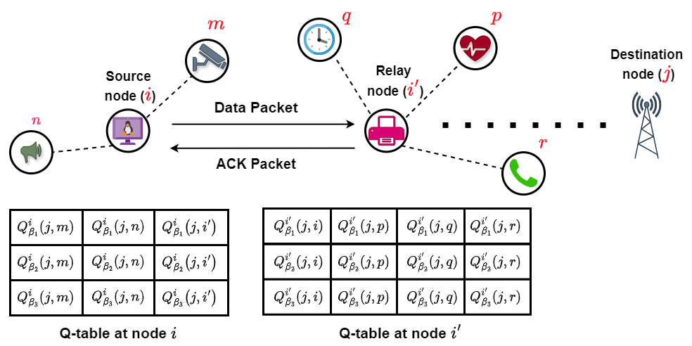
Figure 1: Depiction of Proposed Distributed DPQ-Learning Routing

VI Experimental Results

We compare the efficiency of the proposed Distributed DPQ-Learning algorithm with six baseline schemes listed below:

1. Reinforcement-Learning-Based Energy Efficient Control and Routing Protocol for Wireless Sensor Networks (RLBEEP) [13]

2. Reinforcement Learning for Life Time Optimization (R2LTO) [14]

3. Reinforcement Learning Based Routing (RLBR) [15]

4. Fuzzy multiobjective routing for maximum lifetime and minimum delay (FMOLD) [3]

5. Recursive Shortest Path Algorithm based Routing (RSPAR) [4]

6. Static MultiObjective Reinforcement-Learning based Routing (SMORLR)

SMORLR is the brute force version of MORL-based routing with the same objectives as the proposed method. But, it starts learning from scratch when new changes occur in preferences.

VI-A The Simulation Setup and Parameters

The experiments are conducted on 11th Gen Intel(R) Core(TM) i7-1185G7 CPU @ 3.00GHz with 32 GB RAM machine with Windows operating system. Experiments use MAC protocols as IEEE 802.15.4, in which the packet size is assumed as $133$ Bytes and the communication overhead per packet is considered as $30$ Bytes. Further, the simulation is operated using a network of $100$ IoT nodes uniformly deployed in a $100m^{2}$ field. During evaluations, various parameters such as $\alpha$, $E_{idle}$, $N$, and $E_{awake}$ are defined as 0.9, 0.5 nJ, 100, and 0.5$\mu J$, respectively. In each simulation, we consider four sets of experiments run five times each under two different scenarios, such as sequential (Experiment 1 & 2) and simultaneous (Experiment 3 & 4) exploration strategies, by varying their frequency of preference variations periodically (every 1000th episode) and frequently (each episode).

The variation of $\epsilon$-values and preference variation are shown in Figure 2. Since experiments 1 and 2 are characterized by sequential exploration and exploitation, the $\epsilon$ value (Figure 2(a)) in the proposed algorithm is $1$ in the first $1000$ episodes (indicating full exploration and no exploitation) and $0$ afterward (indicating no exploration and only exploitation). In experiments $3$ and $4$ (Figure 2(b)), the $\epsilon$ is set as $1$ in the beginning and then linearly reduced to $0$, thus achieving the desired simultaneous exploration and exploitation. In all the experiments, the $\epsilon$ values for the SMORLR baseline are reset to $1$ each time the decision-maker changes the preference. Then, it linearly reduces to $0$, encouraging fresh exploration after each preference-change. The frequency of preference variation is a thousand episodes in experiments $1$ and $3$ (Figure 2(c)), and each episode in experiments $2$ and $4$ (Figure 2(d)). The two different preference variation patterns are considered to study the effect of the frequency of preference changes on performance.

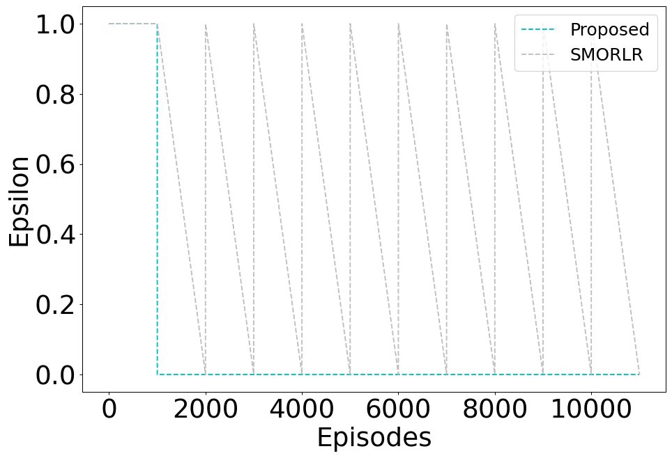
(a) Epsilon variation in experiments 1 and 2

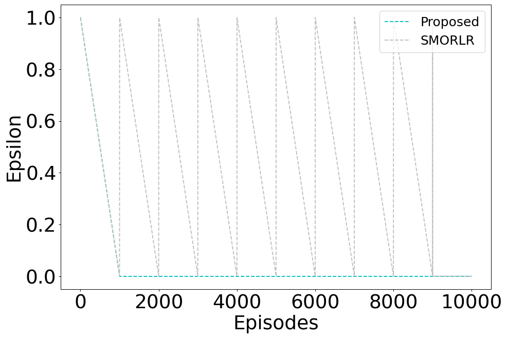
(b) Epsilon variation in experiments 3 and 4

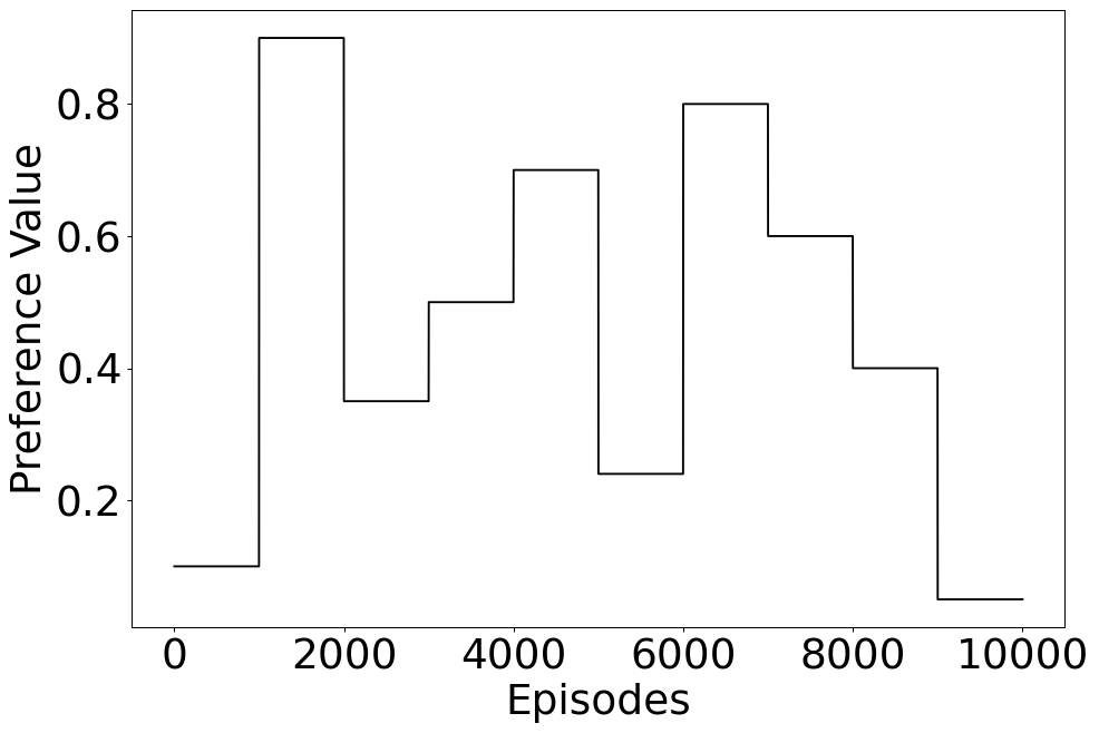
(c) Preference Variation in experiments 1 and 3

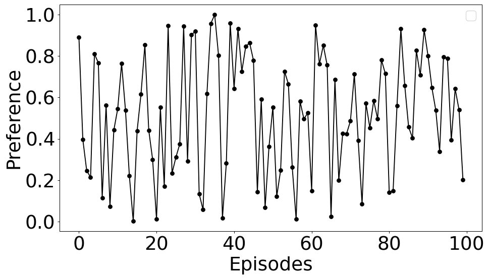
(d) Preference Variation in experiments 2 and 4

Figure 2: Variation of Epsilon and Preferences during the experimental simulations.

We compare the performance of the proposed Distributed DPQ-Learning routing algorithm with the six baselines on three vital metrics: overall reward, packet delivery, and energy consumption. The following subsections provide detailed analysis of these three metrics under sequential and simultaneous exploration-exploitation scenarios.

VI-B Sequential Exploration and Exploitation

We provide a detailed performance analysis of the proposed work based on a sequential exploration and exploitation scheme with varying frequency of preference variation at every thousandth episode (in Experiment 1) and every episode (in Experiment 2). In the below subsections, we compare the performance of the proposed work and baseline algorithms using overall reward, packet delivery, and energy consumption.

VI-B1 Overall Reward

The overall reward captures the optimization goal by comprising both objectives as per the current episode’s preference $\beta_{m}$. At an episode $m$, when the state is $s$, and a routing action $a$ is taken, the overall reward is $r^{\texttt{Overall}}$ is defined as:

$$r^{\texttt{Overall}}(s,a)=\beta_{m}r^{\texttt{Energy}}(s,a)+(1-\beta_{m})r^{\texttt{PDR}}(s,a)$$ (6)

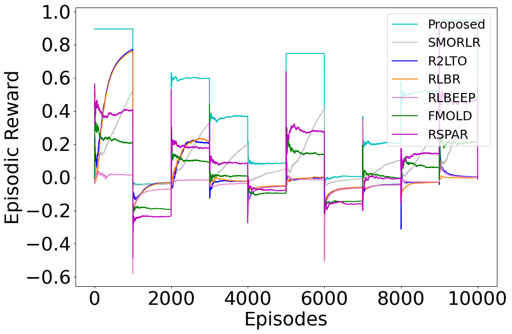
(a) Experiment 1: Comparison of the episodic rewards

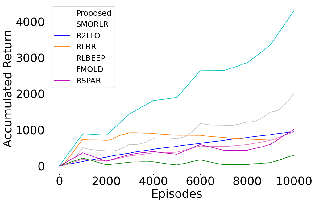
(b) Experiment 1: Comparison of accumulated returns

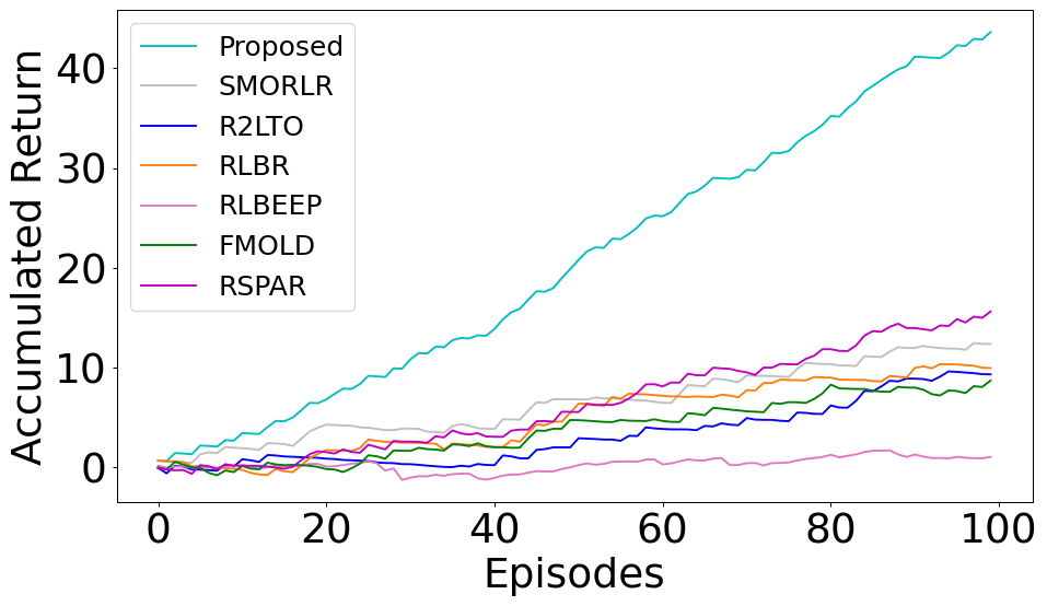
(c) Experiment 2: Accumulated Return v/s Episodes

Figure 3: Overall reward in Sequential exploration-exploitation scheme.

Figure 3 shows the performance comparison of $r^{\texttt{Overall}}(s,a)$ in the sequential exploration-exploitation scheme between the proposed and existing works. Figure 3(a) and Figure 3(b) shows experiment 1’s episodic and accumulated rewards, respectively. Figure 3(a) shows that the proposed Distributed DPQ-Learning routing algorithm immediately adapts according to the preference and gives high performance even if the preferences change. This superior performance is attributed to the Pareto front, which is learned during the exploration phase. In contrast SMORLR starts learning the policy suited to the new preference after each preference shift. Although it focuses on the same objectives, it still does not learn enough to outperform the proposed dynamic protocol after 1000 episodes of learning. Static protocols perform poorly in environments where preferences change dynamically. Algorithms like R2LTO, RLBR, and RLBEEP, which are primarily energy-focused and static, display performance that is relatively similar to one another for most preferences. However, they underperform by an average of 102% compared to the proposed approach. During the intervals between $1000-2000$ and $6000-7000$ episodes, these algorithms begin to show improvement, as the preference weight, $\beta$, shifts to $0.1$ and $0.2$, giving higher priority to energy efficiency–an objective for which they are optimized. RSPAR underperforms by 263% on average compared to the proposed method, while FMOLD, despite being a multi-objective approach, is 266% less efficient. Moreover, they don’t seem to be learning efficient policies with time. However, the proposed algorithm performs better immediately (from the beginning of these intervals) because it utilizes the Pareto front learned during exploration.

The cumulative reward is shown in Figure 3(b), and confirm superiority in the proposed distributed DPQ-Learning algorithm over baseline approaches over the long run. Through the episodes, this outperformance becomes increasingly evident. Finally, after 10000 episodes, we can notice that the accumulated return for the proposed method is better than SMORLR by $2.3\times$, RLBEEP by $5.12\times$, R2LTO and FMOLD by $5.25\times$, RLBR by $6\times$, and RSPAR by $16.8\times$. Similarly, in experiment 2, preferences were randomly changed in each episode and the measured performance is shown in Figure 3(c). Here we noticed that the accumulated returns of the proposed routing protocol are consistently higher than baselines, and the difference becomes larger with more episodes. At the end of $100$ episodes, the accumulated return of the proposed algorithm is around $43$ which is $3.3\times$ of RSPAR, $4.3\times$ of SMORLR, $6.14\times$ of RLBR, $7.16\times$ of R2LTO, $8.6\times$ of FMOLD and $43\times$ of RLBEEP. Our observations confirm the proposed method consistently outperforms all baselines and adapts to this efficient performance irrespective of preference changes.

VI-B2 Energy

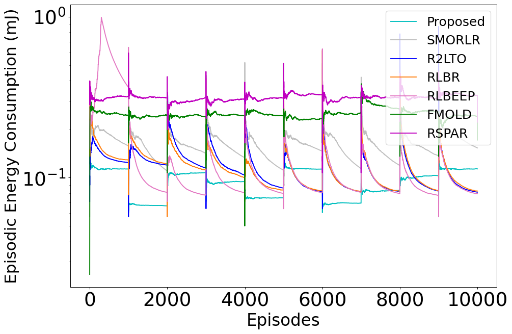
(a) Experiment 1: Episodic Energy Consumption

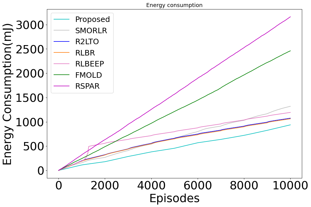
(b) Experiment 1: Comparison of total energy consumption

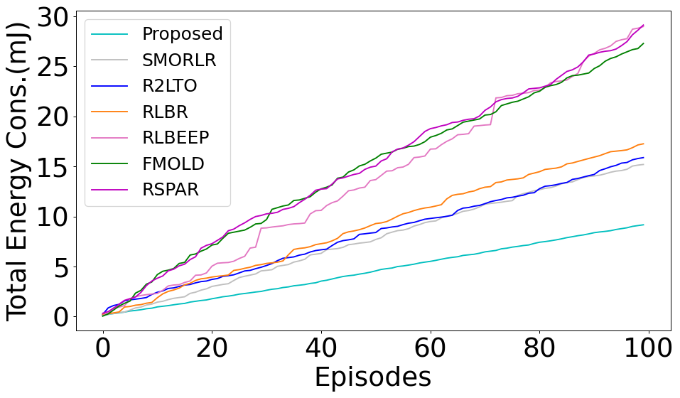
(c) Experiment 2: Total Energy consumption v/s Episodes

Figure 4: Energy Consumption in the Sequential exploration-exploitation scheme.

Figure 4(a) compares episodic energy consumption (in mJ) across baseline algorithms over $10,000$ episodes, showing their performance trends. The Y-axis in Figure 4(a) is logarithmic, ranging from $0$ to $1$ mJ. The proposed distributed DPQ-Learning routing protocol leads to minimal episodic energy consumption whenever a higher preference is given to the energy objective while performing reasonably well even when the preference for the energy objective is low. On average, the proposed distributed DPQ-Learning routing protocol shows about $80-90$% lower energy consumption than baseline algorithms. SMORLR consumes around $150-200\%$ more energy than the proposed algorithm over time. However, with each preference change, it starts to learn to converge closer to the proposed algorithm gradually. However, the more often preferences change, the inefficient this approach becomes. R2LTO and RLBR tend to stabilize close to $0.3$ mJ of episodic energy consumption, with about $50\%$ higher consumption than the proposed method. RLBEEP spikes at first and then stabilizes around $0.4$ mJ. It has approximately $100\%$ higher consumption than the proposed algorithm. FMOLD stabilizes near $0.6$ mJ, about $3$ times the energy of the distributed DPQ-Learning approach. The energy consumption is the highest among the four, but the consistency is better than RSPAR. The lowest energy efficiency can be seen in [RSPAR], which spikes above $1$ mJ initially and stabilizes around $0.8$ mJ. Its energy consumption is $4\times$ to $5\times$ higher than the proposed algorithm. Although RLBEEP, R2LTO, and RLBR learn to perform well or better than the proposed method for certain sets of preferences, but their overall performance over a long period is lesser than the proposed method.

The cumulative effects over the long run can be more clearly seen in Figure 4(b), which depicts the cumulative energy consumption over episodes. The figure shows that the proposed algorithm is the most energy-efficient, consuming $30-50\%$ lesser energy than SMORLR, RLBEEP, RLBR, and R2LTO, and around $4\times$ and $3.4\times$ less than RSPAR and FMOLD respectively by episode $10000$. While SMORLR, RLBEEP, R2LTO, and RLBR perform moderately well, RSPAR and FMOLD exhibit the highest cumulative energy consumption, highlighting their inefficiency. However, the proposed routing algorithm still consumes less energy than any baseline algorithm. Similarly we continue our evaluations in Experiment 2, where preferences were randomly changed in each episode. As shown in Figure 4(c), the cumulative energy consumption for the proposed routing protocol is lesser than those of the baseline methods, with the gap widening as more episodes progress. By the end of 100 episodes, we find that the cumulative energy consumption of RSPAR and RLBEEP is $3.87\times$, FMOLD is $3.53\times$, RLBR is $2\times$, R2LTO is $1.73\times$, and SMORLR is $1.67\times$ that of the proposed routing scheme. Therefore, regardless of the exploration policy or preference variation patterns, the proposed method leads to a substantially lesser amount of energy consumption than the baseline algorithms.

VI-B3 Packet Delivery

Figure 5(a) and Figure 5(b) depict the variation in episodic and cumulative packet deliveries, respectively. Figure 5(a) shows that the proposed distributed DPQ-Learning routing algorithm outperforms all the baselines for episodes ($0-1000,2000-4000,5000-6000,7000-10000$) where the preference for the PDR objective is more than 0.5. RSPAR and FMOLD tend to hover around episodic PDR of $0.4-0.5$ and $0.3-0.4$ respectively. SMORLR tends to learn with time to maximize the PDR for each new preference vector. However, its peak performances are $50\%$ lower than the proposed method’s consistent performances. RLBEEP, R2LTO, and RLBR focus on the energy aspect of the system and did not consider PDR. As a result, they consistently ignore this objective and performing worse. At the beginning, R2LTO and RLBR seem to perform fairly well against PDR, but eventually, they start performing poorly as well.

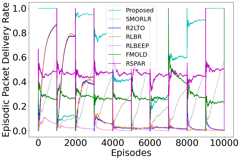
(a) Experiment 1: Episodic PDR

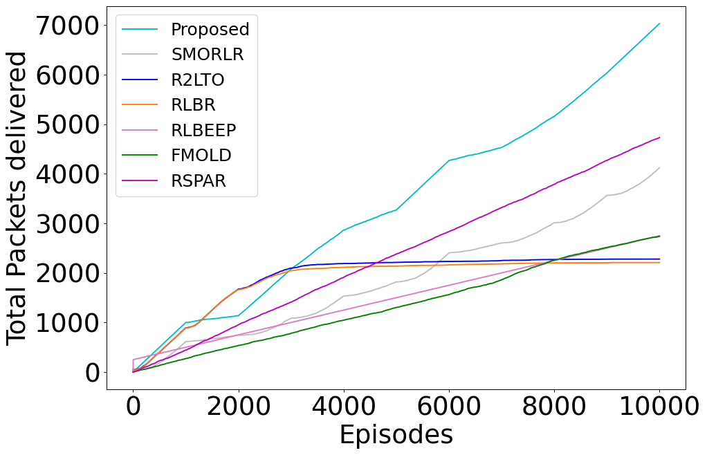
(b) Experiment 1: Comparison of no. of packets delivered

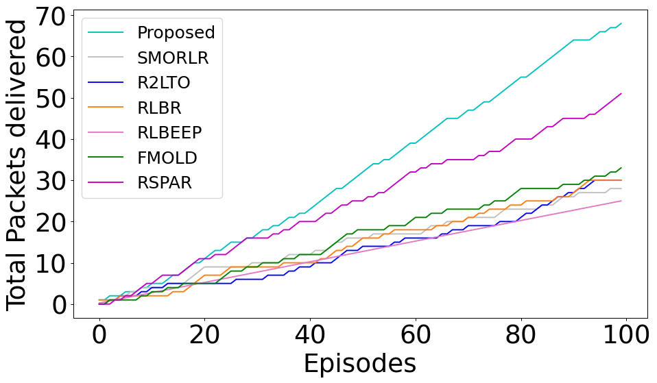
(c) Experiment 2: Total Packets Delivered v/s Episodes

Figure 5: PDR in the Sequential exploration-exploitation scheme.

We analyze cumulative packet delivery over a long run as shown in Figure 5(b), and the proposed method consistently outperforms all the baselines except for some initial fluctuations durations. As time passes, the difference between performances becomes more evident. At the end of $10000$ episodes, the proposed method has better performance than RSPAR by around $1.78\times$, FMOLD and RLBEEP by $3\times$, and R2LTO and RLBR by around $3.5\times$. Similar results were observed in Experiment 2, where preferences were randomly changed in each episode as shown in Figure 5(c). We observe here that the total number of packets delivered by the proposed work consistently exceeds those delivered by the baseline method, and that the gap widens as more episodes are completed. By the end of $100$ episodes, the proposed algorithm’s accumulated return reaches approximately $68$, which is $1.41\times$ that of RSPAR, $2.6\times$ greater than FMOLD, $2.62\times$ better than R2LTO and RLBR, $2.83\times$ higher than SMORLR, and $3.1\times$ higher than RLBEEP. Consequently, regardless of the exploration policy or preference variation patterns, the proposed method outperforms the baseline algorithms in terms of PDR.

VI-C Simultaneous Exploration and Exploitation

We further extended our experiments using a Simultaneous exploration and exploitation approach with varying frequency of preference variation at every thousandth episode (in Experiment $3$) and every episode (in Experiment $4$). Similar to previous subsection, we evaluate the performance of the proposed Distributed DPQ-Learning routing algorithm against the six baseline routing algorithms based on three key criteria: overall reward, packet delivery, and energy consumption.

VI-C1 Overall Reward

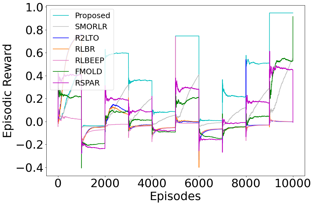
(a) Experiment 3: Comparison of the episodic rewards

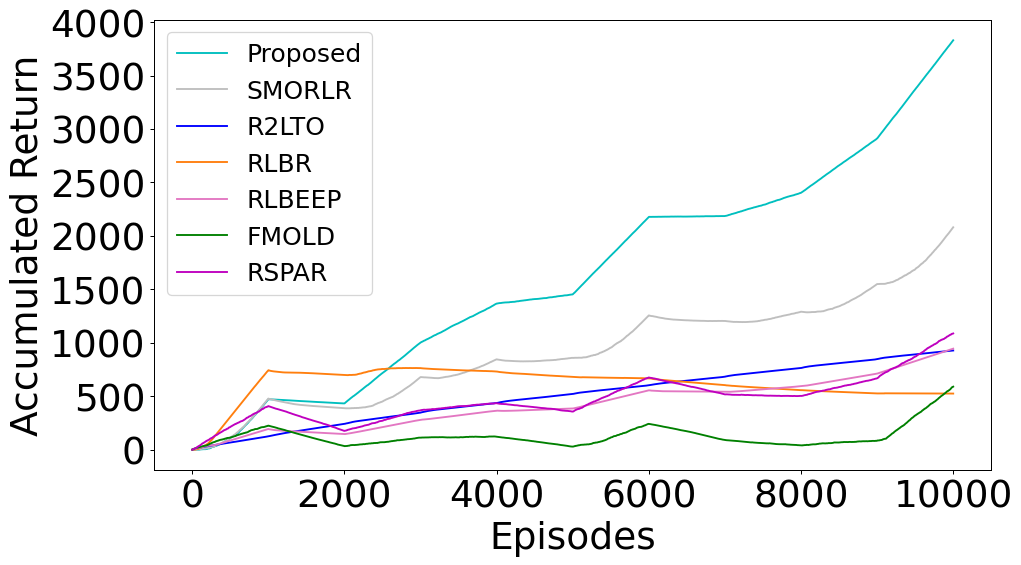
(b) Experiment 3: Comparison of accumulated returns

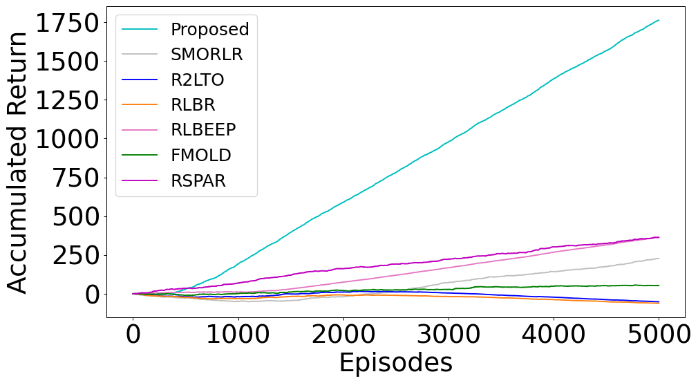
(c) Experiment 4: Accumulated Return v/s Episodes

Figure 6: Overall Reward in the Simultaneous exploration-exploitation scheme.

We present both episodic rewards (figure 6(a)) and accumulated returns (figure 6(b)) of the proposed Distributed DPQ-Learning routing algorithm against the six baseline routing algorithms. From figure 6(a), we can observe that the proposed Distributed DPQ-Learning routing algorithm learns to optimize the overall return by doing more exploration than exploitation in the first $1000$ episodes. The pareto front is also learned in this phase. In contrast to the sequential exploration-exploitation scheme, the simultaneous scheme involves both exploration and exploration occurring hand-in-hand while gradually reducing exploration and increasing exploitation. From figure 6(a), we notice the performance of the proposed Distributed DPQ-Learning routing algorithm may not be superior in the beginning phases of exploration, but after a few exploration ($1000$ episodes), it outperforms all the baselines with respect to episodic rewards. The proposed protocol also dynamically and immediately adjusts to changing preferences after a few explorations, while other baselines fail to do so. For example, SMORLR learns to adapt after each preference change. However, the process is slow, and the preferences change before it can adapt to match the proposed protocol’s performance. Further, R2LTO, RLBEEP, FMOLD, and RLBR consistently focus on a fixed objective preference, mostly prioritizing energy efficiency. They tend to learn certain intervals to increase returns, but they still fall short of the proposed method by $12-13\times$ approximately. RSPAR performs, on average, 344% less efficiently than the proposed approach. Thus, while certain baseline methods may perform well under specific preferences, the proposed algorithm consistently outperforms them and adapts quickly to changing preferences.

Figure 6(b) illustrates cumulative performance over time. Initially, all (baseline and proposed) algorithms start with zero cumulative returns. At the beginning, RSPAR and RLBR outperform the proposed DPQ-Learning algorithm. However, after a few explorations, the proposed approach starts utilizing the learned Pareto front and consistently outperforms the baselines, with the performance gap widening as more episodes are completed. Figure 6(b) shows that after $10,000$ episodes, the accumulated return of the proposed method surpasses SMORLR by $111.11\%$, RSPAR by $322.22\%$, R2LTO and RLBEEP by $375\%$, FMOLD by $850\%$, and RLBR by $927\%$ approximately. Similarly, significant improvements were seen in Experiment $4$, where preferences were randomly altered in each episode. Figure 6(c) shows that the proposed routing protocol consistently achieves significantly higher accumulated returns than the baseline, with the performance gap growing as episodes progress. By the end of $5000$ episodes, the proposed algorithm achieves an accumulated return of around $1750$, which is $5.48\times$ that of RSPAR and RLBEEP, $8.21\times$ that of SMORLR, $34\times$ that of FMOLD, and $36\times$ that of R2LTO and RLBR. Based on these results, we observe that the proposed method consistently outperforms all baselines in terms of overall returns and adapts rapidly to changes in preferences regardless of exploration policy.

VI-C2 Energy

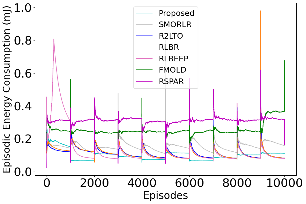
(a) Experiment 3: Episodic Energy Consumption

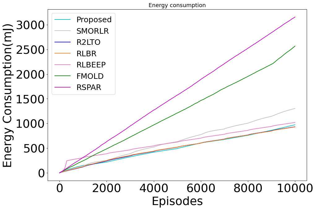
(b) Experiment 3: Comparison of total energy consumption.

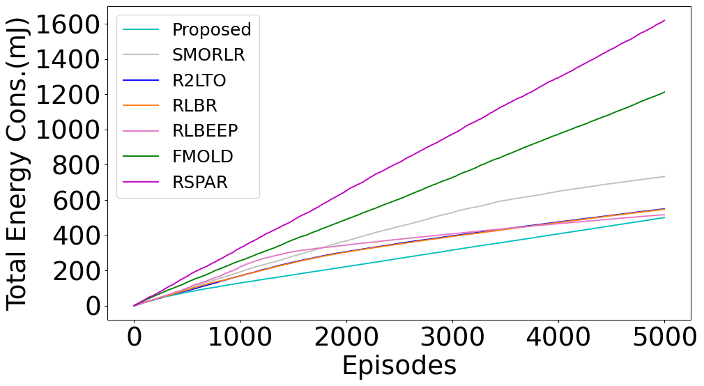
(c) Experiment 4: Total Energy Consump. v/s Episodes

Figure 7: Energy Consumption in the Simultaneous exploration-exploitation scheme.

In this subsection, we assess the energy-efficiency of the proposed and baseline routing algorithms on individual objectives when preferences between them change periodically and frequently. Figure 7(a) highlights the episodic energy consumption (in mJ) across various routing algorithms over $10,000$ episodes, where the preference changes after every $1000$ episode. On average, the proposed distributed DPQ-Learning routing protocol demonstrates $65-80$% lower energy consumption than the other routing protocols. The proposed approach consumed the minimum energy whenever a higher preference was given to the energy objective (intervals $1000-2000,4000-5000,and6000-8000$) while performing reasonably well even when the preference for the energy objective was lower. On average, SMORLR consumes approximately $80\%$ more energy than the proposed method, although it gradually converges closer to it with each preference shift. However, the more frequently preferences change, the less efficient SMORLR becomes. R2LTO, RLBEEP, and RLBR consume around $60\%$ more energy than the proposed method. Since they focus primarily on energy considerations, they perform the highest among baselines. However, the proposed approach outperforms them because of a more efficient reward formulation. FMOLD consumes around $160\%$ more energy than the proposed method while maintaining a consistent performance. RSPAR exhibits the energy inefficiency $\approx 200\%$ more energy consumption than the proposed algorithm.

The cumulative energy consumption shown in Figure 7(b) indicate that after 10000 episodes, the cumulative energy consumption of the proposed method is very close to RLBEEP, R2LTO, and RLBR with the value of around $700$ mJ, which is $48.5\%$ lesser than that of SMORLR and $242.85\%$ less than that of FMOLD, and $242.85\%$ less than that of RSPAR. While SMORLR, RLBEEP, R2LTO, and RLBR perform reasonably well because of energy considerations in their RL reward formulations. Whereas RSPAR and FMOLD exhibit the highest cumulative energy consumption, underscoring their inefficiency. The plots demonstrate that even when energy is assigned to a lower preference, the overall energy consumption of the proposed routing protocol is still relatively low or equal to most baselines. A similar trend was observed in Experiment 4, where preferences were randomly altered in each episode. As seen in Figure 7(c), the proposed routing protocol’s cumulative energy consumption remains more efficient than that of the baseline methods, with the gap increasing as the episodes progress. After $5000$ episodes, the cumulative energy consumption of the proposed distributed DPQ-Learning routing algorithm is $78.125\%$ lower than that of RSPAR, $66.35\%$ lower than that of FMOLD, $41.67\%$ lower than that of SMORLR, $12.5\%$ lower than that of R2LTO, and RLBR, and $3\%$ lower than that of RLBEEP. Therefore, the proposed method consumes significantly less energy than baseline algorithms regardless of exploration strategy or preference shifts. Whenever an energy objective is given higher priority, the method consumes the least amount of energy and performs reasonably well even when the energy objective is given a lower priority.

VI-C3 Packet Delivery

Here, we assess PDR of the proposed and baseline algorithms on individual objectives when preferences between them change periodically (every 1000 episodes) and frequently (each episode). Figures 8(a) and 8(b) illustrate variations in episodic and cumulative packet deliveries, respectively. From Figure 8(a), it is evident that after a certain duration of exploration ($1000$ episodes), the proposed distributed DPQ-Learning routing algorithm outperforms all baselines in episodes where the preference for the PDR objective exceeds 0.5. In comparison, RSPAR and FMOLD maintain episodic PDR levels of around 0.4-0.5 and 0.2-0.3, respectively. Although SMORLR gradually learns to maximize PDR with each new preference vector, its peak performance remains 50% lower than the consistent results achieved by the proposed algorithm (after the exploration period). Meanwhile, RLBEEP, R2LTO, and RLBR primarily focus on energy optimization and disregard the PDR objective, which consistently underperforms. Initially, R2LTO and RLBR demonstrate reasonable PDR performance, but it deteriorated over time.

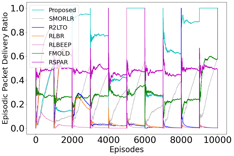
(a) Experiment 3: Episodic PDR

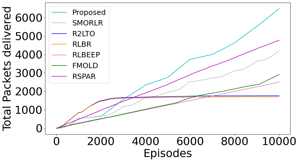
(b) Experiment 3: Comparison of total packets delivered

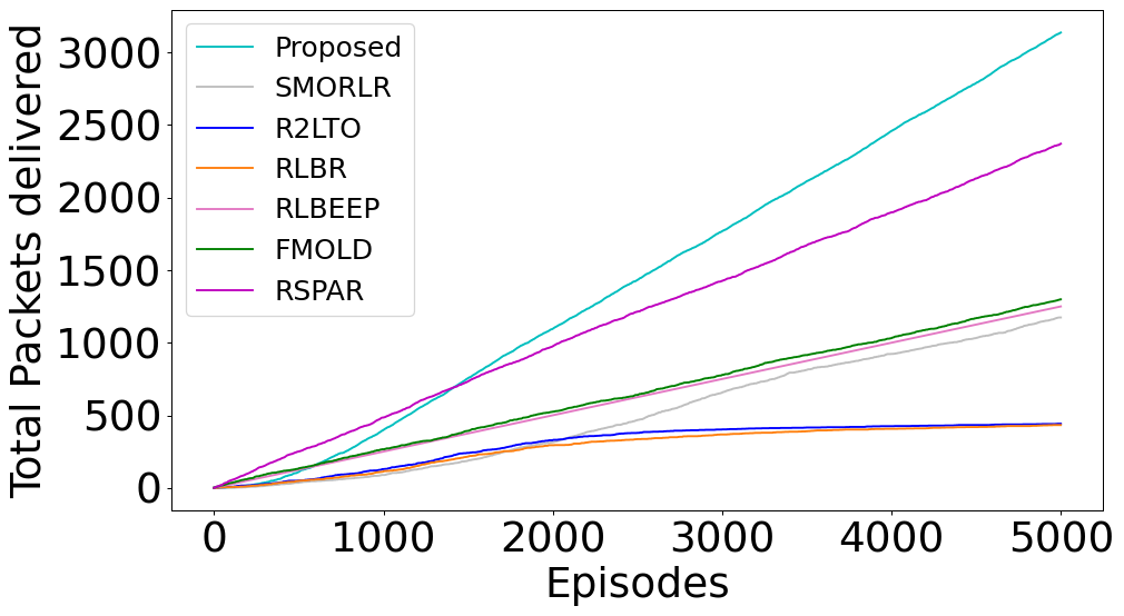
(c) Experiment 4: Total Packets Delivered v/s Episodes

Figure 8: Packet Delivery rate in the Simultaneous exploration-exploitation scheme.

Figure 8(b) provides a more comprehensive view by showcasing cumulative packet delivery, which offers a fair comparison over the long run. The proposed method starts outperforming all baselines, after $3000$ episodes of sufficient learning. As time progresses, the performance gap widens. By the end of $10,000$ episodes, the proposed method delivers $46.67\%$ more packets than RSPAR, $69.23\%$ more packets than SMORLR, $164\%$ more packets than FMOLD, $230\%$ more packets than RLBR, and $255.12\%$ more packets than R2LTO and RLBEEP. Similar results were seen in Experiment 4, where preferences were randomly changed in each episode. As depicted in Figure 8(c), the total number of packets delivered by the proposed routing protocol consistently and significantly exceeds those of the baselines, with the gap widening as more episodes are completed. Specifically, at the end of $5000$ episodes, the total packet delivery for the proposed algorithm reaches around $3200$, which is $33.33\%$ more than RSPAR, around $166\%$ more than FMOLD and RLBR, $220\%$ more than SMORLR, and $814.3\%$ more than more than RLBEEP and R2LTO. The proposed method outperforms all baselines when the preference for PDR objective is higher, and is also acceptable for preferences at lower levels.

VII Conclusions

This paper presents a dynamic and distributed IoT routing protocol based on multi-objective Q-learning, designed to adapt to changing priorities in real-time. This approach optimizes key metrics like overall reward, energy efficiency and PDR. By leveraging distributed learning at individual nodes, the method avoids the need for centralized control, enhancing scalability and robustness. Simulations show that this approach outperforms existing algorithms in adaptability, energy efficiency, and packet delivery. The proposed approach shows consistent out-performance irrespective of the exploration strategies, and preference change patterns. The study highlights the potential of reinforcement learning for dynamic IoT networks and suggests future work on extending the algorithm to address security and more complex objectives. This makes it a promising solution for real-time, flexible routing in evolving IoT environments.

Shubham Vaishnav is currently pursuing Ph.D. at the Department of Computer and Systems Science, Stockholm University, Sweden. This research program is funded by Digital Futures. He received Bachelors’ and Masters’ degrees in Computer Science and Engineering from the Indian Institute of Technology (Indian School of Mines), Dhanbad. His research interests include Multiobjective and Adaptive decision-making in IoT and Edge networks, Reinforcement learning, Federated Learning, and data-driven decision-making in critical societal infrastructure.

Praveen Kumar Donta (SM’22), senior lecturer at the Department of Computer and Systems Sciences, Stockholm University, Sweden. Earlier, he was a Postdoctoral researcher at Distributed Systems Group, TU Wien, Vienna, Austria. He received his Ph. D. at the Indian Institute of Technology (Indian School of Mines), Dhanbad, from the Department of Computer Science and Engineering in May 2021. He is a visiting PhD student at the University of Tartu, Estonia, during his PhD for six months. He received his Bachelor’s and Master’s in Technology from JNT University, Anantapur, India. He is an Editorial Board member for IEEE IoT Journal, Nature Scientific Reports, Computing Springer, ETT Wiley, and PLOS One. His current research includes the Learning techniques for Distributed Computing Continuum Systems, Sensor Networks, the Internet of Things, and Edge Intelligence.

Sindri Magnússon is an Associate Professor in the Department of Computer and Systems Science at Stockholm University, Sweden. He received a B.Sc. degree in Mathematics from the University of Iceland, Reykjav´ık Iceland, in 2011, a Masters degree in Applied Mathematics (Optimization and Systems Theory) from KTH Royal Institute of Technology, Stockholm, Sweden, in 2013, and the PhD in Electrical Engineering from the same institution, in 2017. He was a postdoctoral researcher 2018-2019 at Harvard University, Cambridge, MA, and a visiting PhD student at Harvard University for 9 months in 2015 and 2016. His research interests include large-scale distributed/parallel optimization, machine learning, and control.

References

- [1] G. Forecast et al., “Cisco visual networking index: global mobile data traffic forecast update, 2017–2022,” Update, vol. 2017, p. 2022, 2019.
- [2] K. Miettinen, Nonlinear Multiobjective Optimization. Kluwer Academic Publishers, 1999.
- [3] M. R. Minhas, S. Gopalakrishnan, and V. C. Leung, “Multiobjective routing for simultaneously optimizing system lifetime and source-to-sink delay in wireless sensor networks,” in IEEE International Conference on Distributed Computing Systems Workshops, 2009, pp. 123–129.
- [4] J. Cota-Ruiz, P. Rivas-Perea, E. Sifuentes, and R. Gonzalez-Landaeta, “A recursive shortest path routing algorithm with application for wireless sensor network localization,” IEEE Sensors Journal, vol. 16, no. 11, pp. 4631–4637, 2016.
- [5] T. A. Al-Janabi and H. S. Al-Raweshidy, “A centralized routing protocol with a scheduled mobile sink-based ai for large scale i-iot,” IEEE Sensors Journal, vol. 18, no. 24, pp. 10 248–10 261, 2018.
- [6] V. Gomathy, N. Padhy, D. Samanta, M. Sivaram, V. Jain, and I. S. Amiri, “Malicious node detection using heterogeneous cluster based secure routing protocol (hcbs) in wireless adhoc sensor networks,” Journal of Ambient Intelligence and Humanized Computing, vol. 11, pp. 4995–5001, 2020.
- [7] A. Ahmed, K. A. Bakar, M. I. Channa, K. Haseeb, and A. W. Khan, “Terp: A trust and energy aware routing protocol for wireless sensor network,” IEEE Sensors Journal, vol. 15, no. 12, pp. 6962–6972, 2015.
- [8] B. Zeng, J. Deng, Y. Dong, X. Yang, L. Huang, and Z. Xiao, “A whale swarm-based energy efficient routing algorithm for wireless sensor networks,” IEEE Sensors Journal, vol. 24, no. 12, pp. 19 964–19 981, 2024.
- [9] S. Yang, L. Zhuang, J. Zhang, J. Lan, and B. Li, “A multipolicy deep reinforcement learning approach for multiobjective joint routing and scheduling in deterministic networks,” IEEE Internet of Things Journal, vol. 11, no. 10, pp. 17 402–17 418, 2024.
- [10] M. Wang, Y. Wei, X. Huang, and S. Gao, “An end-to-end deep reinforcement learning framework for electric vehicle routing problem,” IEEE Internet of Things Journal, vol. 11, no. 20, pp. 33 671–33 682, 2024.
- [11] X. Guo, H. Lin, Z. Li, and M. Peng, “Deep-reinforcement-learning-based qos-aware secure routing for sdn-iot,” IEEE Internet of Things Journal, vol. 7, no. 7, pp. 6242–6251, 2020.
- [12] M. U. Younus, M. K. Khan, and A. R. Bhatti, “Improving the software-defined wireless sensor networks routing performance using reinforcement learning,” IEEE Internet of Things Journal, vol. 9, no. 5, pp. 3495–3508, 2022.
- [13] A. F. E. Abadi, S. A. Asghari, M. B. Marvasti, G. Abaei, M. Nabavi, and Y. Savaria, “Rlbeep: reinforcement-learning-based energy efficient control and routing protocol for wireless sensor networks,” IEEE Access, vol. 10, pp. 44 123–44 135, 2022.
- [14] S. E. Bouzid, Y. Serrestou, K. Raoof, and M. N. Omri, “Efficient routing protocol for wireless sensor network based on reinforcement learning,” in 2020 5th International Conference on Advanced Technologies for Signal and Image Processing (ATSIP). IEEE, 2020, pp. 1–5.
- [15] W. Guo, C. Yan, and T. Lu, “Optimizing the lifetime of wireless sensor networks via reinforcement-learning-based routing,” International Journal of Distributed Sensor Networks, vol. 15, no. 2, p. 1550147719833541, 2019.
- [16] L. Yang, Y. Wei, F. R. Yu, and Z. Han, “Joint routing and scheduling optimization in time-sensitive networks using graph-convolutional-network-based deep reinforcement learning,” IEEE Internet of Things Journal, vol. 9, no. 23, pp. 23 981–23 994, 2022.
- [17] Y.-R. Chen, A. Rezapour, W.-G. Tzeng, and S.-C. Tsai, “Rl-routing: An sdn routing algorithm based on deep reinforcement learning,” IEEE Transactions on Network Science and Engineering, vol. 7, no. 4, pp. 3185–3199, 2020.
- [18] D. M. Casas-Velasco, O. M. C. Rendon, and N. L. S. da Fonseca, “Drsir: A deep reinforcement learning approach for routing in software-defined networking,” IEEE Transactions on Network and Service Management, vol. 19, no. 4, pp. 4807–4820, 2022.
- [19] C. Liu, M. Xu, Y. Yang, and N. Geng, “Drl-or: Deep reinforcement learning-based online routing for multi-type service requirements,” in IEEE INFOCOM 2021 - IEEE Conference on Computer Communications, 2021, pp. 1–10.
- [20] W.-x. Liu, J. Cai, Q. C. Chen, and Y. Wang, “Drl-r: Deep reinforcement learning approach for intelligent routing in software-defined data-center networks,” Journal of Network and Computer Applications, vol. 177, p. 102865, 2021.
- [21] L. Chen, B. Hu, Z.-H. Guan, L. Zhao, and X. Shen, “Multiagent meta-reinforcement learning for adaptive multipath routing optimization,” IEEE Transactions on Neural Networks and Learning Systems, vol. 33, no. 10, pp. 5374–5386, 2021.
- [22] J. Rischke, P. Sossalla, H. Salah, F. H. Fitzek, and M. Reisslein, “Qr-sdn: Towards reinforcement learning states, actions, and rewards for direct flow routing in software-defined networks,” IEEE Access, vol. 8, pp. 174 773–174 791, 2020.
- [23] P. Cong, Y. Zhang, Z. Liu, T. Baker, H. Tawfik, W. Wang, K. Xu, R. Li, and F. Li, “A deep reinforcement learning-based multi-optimality routing scheme for dynamic iot networks,” Computer Networks, vol. 192, p. 108057, 2021.
- [24] K. Ergun, R. Ayoub, P. Mercati, and T. Rosing, “Reinforcement learning based reliability-aware routing in iot networks,” Ad Hoc Networks, vol. 132, p. 102869, 2022.
- [25] H. Farag and c. Stefanovic, “Congestion-aware routing in dynamic iot networks: A reinforcement learning approach,” in 2021 IEEE Global Communications Conference (GLOBECOM), 2021, pp. 1–6.
- [26] Y.-R. Chen, A. Rezapour, W.-G. Tzeng, and S.-C. Tsai, “Rl-routing: An sdn routing algorithm based on deep reinforcement learning,” IEEE Transactions on Network Science and Engineering, vol. 7, no. 4, pp. 3185–3199, 2020.
- [27] Q. He, Y. Wang, X. Wang, W. Xu, F. Li, K. Yang, and L. Ma, “Routing optimization with deep reinforcement learning in knowledge defined networking,” IEEE Transactions on Mobile Computing, vol. 23, no. 2, pp. 1444–1455, 2024.
- [28] L. Huang, M. Ye, X. Xue, Y. Wang, H. Qiu, and X. Deng, “Intelligent routing method based on dueling dqn reinforcement learning and network traffic state prediction in sdn,” Wireless Networks, pp. 1–19, 2022.
- [29] T. V. Phan and T. Bauschert, “Deepair: Deep reinforcement learning for adaptive intrusion response in software-defined networks,” IEEE Transactions on Network and Service Management, vol. 19, no. 3, pp. 2207–2218, 2022.
- [30] S. Javanmardi, M. Shojafar, R. Mohammadi, M. Alazab, and A. M. Caruso, “An sdn perspective iot-fog security: A survey,” Computer Networks, vol. 229, p. 109732, 2023.
- [31] S. Natarajan and P. Tadepalli, “Dynamic preferences in multi-criteria reinforcement learning,” in Proceedings of the 22nd international conference on Machine learning, 2005, pp. 601–608.
- [32] S. Mahadevan, “To discount or not to discount in reinforcement learning: A case study comparing r learning and q learning,” in Machine Learning Proceedings 1994. Elsevier, 1994, pp. 164–172.
- [33] P. Tadepalli, D. Ok et al., “H-learning: A reinforcement learning method to optimize undiscounted average reward,” 1994.
- [34] D. Bertsekas, Dynamic programming and optimal control: Volume I. Athena scientific, 2012, vol. 4.
- [35] R. S. Sutton, A. G. Barto et al., “Reinforcement learning,” Journal of Cognitive Neuroscience, vol. 11, no. 1, pp. 126–134, 1999.