A Holographic, Hydrodynamic Model of a Schwarzschild Black Hole

Abstract

Schwarzschild (non-rotating and chargeless) black holes are classically understood to be voids of extreme gravitation. In this study, we propose a holographic model for their interiors, envisioning them instead as a hydrodynamic medium. Motivated by the neutrino composition in Hawking radiation (81%), we model the interior as a degenerate fluid, mirrored by the horizon via AdS/CFT duality. A Schwarzschild metric revised with a signum function as the power of the ratio $r_{S}/r$ distinguishes interior linear-well dynamics from exterior Schwarzschild geometry, rimming the horizon with singularity-like gravitational attraction. A Hamiltonian analysis of the total action leads to formulating a Schrödinger-like equation, which offers an alternative representation as the contracted Einstein field equations under a holographic-hydrodynamic framework. This eventually yields an equation of state between holographic pressure and black hole mass density: $P=\rho/9$. Ideal gas analysis reveals a total particle count of $\sim 2.8$ times the number of horizon quantum areas, with the Fermi energy far exceeding the Hawking thermal energy, ensuring degeneracy. As our discussion, we explore the mass shell free-fall model of a BH with holographic pressure, and dissect the spherical wave solutions to the Schrödinger-like equation describing confined interior fields and freely propagating exterior quanta (i.e., Hawking radiation).

1 Introduction

Black holes (BHs) as described by general relativity are regions of extreme curvature where the event horizon at $r_{S}=2GM$ ($c=1$) and the geometric center impose mathematical singularities [1, 2, 3]. More contemporary approaches that utilize quantum field theory, string theory, and viscous hydrodynamics remove the event horizon singularity in lieu of a non-trivial boundary manifold (i.e., the black brane) [4, 5, 6, 7, 8, 9, 10, 11, 12, 13, 14, 15, 16, 17, 18]. Implying both AdS/CFT and the holographic principle [8, 9], the information encoded on the black brane corresponds to a mirrored conformal bulk – a holographic fluid – below the surface.

Previous mirror bulk models of BHs include the Bose-Einstein condensate of gravitons [19, 20, 21, 22], a bosonic superfluid [23], and a thermal bath [24]. The boson superfluid and thermal bath models were applied to late-stage evaporating black holes with a thermal noise-inducing temperature $T\propto 1/M$. However, Hawking radiation emitted from the horizon surface – hypothesized to consist 81% neutrinos, 17% photons, and 2% gravitons [25] – gives insight to another BH mirror bulk that is fermionic in structure while also containing bosonic degrees of freedom. Allowing the Hawking particles to mirror the holographic bulk beneath the horizon, we propose a reinterpretation of the interior as a holographic fermionic medium, motivated by the neutrino-dominated composition of Hawking radiation, and consistent with AdS/CFT duality. Unlike bosonic models suited to late-stage evaporation, a hypothetical fermionic medium intends to leverage a Pauli degeneracy pressure as a natural regulator of evaporation rates, aligning qualitatively with known constraints on Hawking evaporation. The insight of the holographic medium’s hydrodynamics, and probing its fermionic degeneracy, is provided in Section 3.

This following work is structured in four sequential sections. However, the remainder of this section, i.e. in Section 1.1, we discuss our metric of choice: a Schwarzschild metric revised with a signum function to distinguish the exterior Schwarzschild geometry from the interior linear well geometry brought by the black 2-brane. A Hamiltonian system construction is laid out in Section 2, utilizing the total action of a black brane $\mathbb{M}$ with a defined boundary $\partial\mathbb{M}$ (i.e., consider the interior geometry) to obtain a field-theoretical Lagrangian. From this Lagrangian, we derive the associating Hamiltonian in the form of a Schrödinger-like equation for the holographic system. After the hydrodynamic insight of the holographic medium in Section 3, Section 4 discusses the solutions to this Schrödinger-like Hamiltonian, as it also depends on the geometry outside the BH horizon, in addition to the mass shell free-fall model of the BH horizon with a non-zero pressure gradient. The latter is to frame BH evaporation due to Hawking radiation as horizon contraction, and how the non-zero pressure gradient contributes to BH evaporation. Finally, we conclude in Section 5.

1.1 Event Horizon as a $n=4$ black 2-brane

Encoding the interior structure in a higher-dimensional holographic framework involves adopting a Tangherlini-like black $p$-brane metric [17, 18]:

$$ds^{2}=\left(\eta_{\gamma\delta}+\frac{r_{S}^{n-p-3}}{r^{n-p-3}}u_{\gamma}u_{\delta}\right)d\sigma^{\gamma}d\sigma^{\delta}+\left(1-\frac{r_{S}^{n-p-3}}{r^{n-p-3}}\right)^{-1}dr^{2}+r^{2}d\Omega^{2}_{n-p-2},$$ (1)

with the dimensions defined by the physical dimensions $n$ and the black brane dimensions $p$. Here, $\eta_{\gamma\delta}$ is the $(p+1)$-Minkowski metric upon the black $p$-brane with the $(-,+\in\mathrm{dim}(p)\,)$ signature, $u^{\gamma}=(1,\vec{0}_{p})$ is the $(p+1)$-flow-velocity, $\sigma^{\gamma}$ is a $(p+1)$-coordinate vector along the black brane, and $d\Omega^{2}_{n-p-2}$ defines the metric of a $(n-p-2)$-sphere.

For a point-like BH ($p=0$) upon $n=4$ physical spacetime, we recover the classic Schwarzschild metric. However, by extending the dimensionality of the black brane into a 2-brane while keeping the spacetime dimension as $n=4$, the event horizon is approximated to resemble a closed spherical surface. This yields an unconventional metric of the following form:

$$ds^{2}=-\left(1-\frac{r}{r_{S}}\right)dt^{2}+\left(1+\left(1-\frac{r}{r_{S}}\right)^{-1}\right)dr^{2}+r^{2}d\Omega^{2}_{0},$$ (2)

where $d\Omega^{2}_{0}=0$ for the 0-sphere (the disjoint union of two points: $S^{0}\simeq\,^{\bullet}\coprod\,\!^{\bullet}$). This metric reveals a linear-well metric with asymptotic flatness at $r=0$; the divergence is instead rimmed along the horizon, i.e. at the coordinate singularity $r=r_{S}$. For a holographic medium that is hydrodynamic, the medium is confined to a linear potential well, with the horizon acting as a gravitational sink where the energy is emitted as Hawking radiation seen by an outside observer. The linear potential well picture of a BH’s interior was approached differently in Ref. [26], which was used as a mathematical tool to describe the noise spectra of Hawking radiation in a Langevin framework.

However, Eq. (2) is an unphysical metric, besides its unconventional form compared to the Schwarzschild metric. The unphysicality of the metric stems from an implied temporial infinity beyond the BH horizon and from a vanished 2-sphere metric, which suggests an absence of spherical symmetry. Correcting this issue by modifying the metric, so that it reads the classic Schwarzschild metric for the exterior $r>r_{S}$ and the $n=4$ black 2-brane for the interior $r<r_{S}$ with a non-zero 2-sphere metric, we define

$$\begin{split}&ds^{2}=-\left(1-\left(\frac{r_{S}}{r}\right)^{\Theta(r)}\right)dt^{2}+\left(1-\left(\frac{r_{S}}{r}\right)^{\Theta(r)}\right)^{-1}dr^{2}+r^{2}d\Omega^{2}_{2},\\ &\Theta(r)=\mathrm{sgn}\left(1-\frac{r_{S}}{r}\right),\end{split}$$ (3)

where $\mathrm{sgn}(x)$ is the signum function of $x$. In the above metric, $\Theta(r)$ gauges the sign of the exponent, which weaves together the Schwarzschild exterior with the linear well interior.

By design, the event horizon at $r=r_{S}$ is the attractive singularity. For external observers, infalling objects will be suspended along the horizon, preserving conventional insight. For internal observers, the holographic medium constituents are instead drawn to the horizon under a linear well profile. For co-moving observers, infalling into the horizon would seem as though under gravitational free-fall, with horizon-rimmed attraction drawing the observer back to the horizon. In this model, what may be Hawking radiation is the information of previous infalling objects huddled along the horizon. A visual aid of the spacetime landscape, plotted by $-g^{00}$ in Eq. (3), is provided in Figure 1, with an associating density plot in Figure 2.

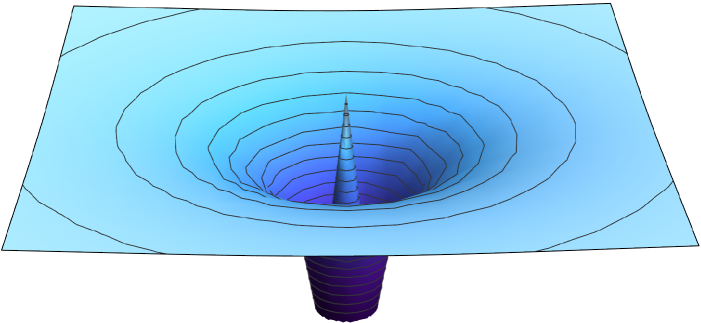
Figure 1: The spacetime manifold for a 2-brane Schwarzschild black hole as depicted by $-g^{00}$ in Eq. (3), with circular contour lines giving a cartographic representation of depth. The conic spike depicting the black hole linear well interior is a consequence to the black 2-brane, illustrating that the horizon is the attractive region.

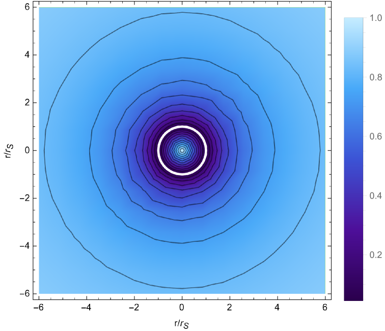
Figure 2: A density plot of the spacetime manifold as depicted by $-g^{00}$ in Eq. (3), with circular contour lines giving a cartographic representation of depth. The color gradient denotes differences in depth, ranging from 0 denoting extreme curvature to 1 denoting flatness. The white ring is the horizon-rimmed singularity.

2 BHs as Hamiltonian Systems

The modified metric (Eq. [3]) redefines the Schwarzschild BH’s event horizon as a black 2-brane in a 4D spacetime, with a linear potential well governing the dynamics of the holographic medium beneath. This geometric framework, inspired by the Tangherlini metric [17], suggests that the horizon encodes the bulk’s quantum information, consistent with the holographic principle [8, 9]. To quantify the dynamics of this medium and its interaction with the horizon, a field-theoretical approach is required.

To model the dynamics of the holographic medium introduced in Section 1, we treat the BH as a Hamiltonian system, with the event horizon as a closed boundary manifold in a 4D spacetime. This approach, rooted in the Arnowitt-Deser-Misner (ADM) formalism [27], allows us to foliate spacetime and analyze the interplay between the horizon’s extrinsic curvature and the bulk’s quantum degrees of freedom. The dynamics of the ADM formalism is governed by the Hamiltonian constraint:

$$\mathcal{H}=\frac{1}{2\sqrt{h}}(h_{ik}h_{jl}-h_{ij}h_{kl})\pi^{ij}\pi^{kl}-\sqrt{h}\,^{(3)}R+\mathcal{H}_{\text{matter}}=0,$$ (4)

where $\pi^{ij}=\sqrt{h}(K^{ij}-Kh^{ij})$ is the conjugate momentum to the induced 3-metric $h_{ij}$, $K_{ij}$ is the extrinsic curvature, and ${}^{(3)}R$ is the 3D Ricci scalar of the hypersurface. Conventionally, the kinetic term $K_{ij}k^{ij}-K^{2}$ drives evolution, while ${}^{(3)}R$ acts as a gravitational potential. For a BH, this describes the interplay between spatial geometry and its embedding in 4D spacetime, with the event horizon as a key boundary.

However, modeling the BH interior as a holographic medium suggests a reinterpretation tailored to holographic hydrodynamics. The high neutrino fraction in Hawking radiation (81%) motivates a fluid dominated by fermionic degrees of freedom, stabilized by Pauli exclusion principle, beneath a black 2-brane horizon. To capture this, we shift focus from the standard ADM formalism to a Lagrangian that reflects the particle’s individual mechanics in the whole system, leveraging the full 4D Ricci scalar and the extrinsic curvature trace $K$. By constructing a total action that combines the Einstein-Hilbert term with the Gibbons-Hawking-York boundary term [6, 7], we derive a Lagrangian to be tailored into a Hamiltonian, which will be applied to the holographic medium.

2.1 Total Action

The total action of a spactime manifold $\mathbb{M}$ with a well-defined boundary $\partial\mathbb{M}$ is constructed by the Einstein-Hilbert action and the Gibbons-Hawking-York boundary action:

$$S_{\text{tot}}=-\frac{1}{16\pi G}\int_{\mathbb{M}}R\sqrt{-g}\,d^{4}x+\frac{\epsilon_{K}}{8\pi G}\oint_{\partial\mathbb{M}}K\sqrt{h}\,d^{3}y.$$ (5)

In the first volume-like integral, $R\equiv g^{\mu\nu}R_{\mu\nu}$ is the trace of the Ricci curvature tensor. A cosmological term $-2\Lambda$ is typically included in the Einstein-Hilbert action for a fuller picture, having $R-2\Lambda$. However, this is neglected, assuming $\Lambda\sim 0$.

In the second surface-like integral, $\epsilon_{K}=+1$ for a spacelike normal on the boundary (appropriate for the horizon), $K=\nabla_{\mu}n^{\mu}$, and $n^{\mu}$ is the unit normal. To rewrite the boundary integral into a volume-like integral, we apply Stokes’ theorem and the identity $1=-n^{\mu}n_{\mu}$:

$$\begin{split}&\frac{-1}{8\pi G}\oint_{\partial\mathbb{M}}K\,n^{\mu}n_{\mu}\,\epsilon_{K}\sqrt{h}\,d^{3}y=\frac{-1}{8\pi G}\oint_{\partial\mathbb{M}}K\,n^{\mu}d\Sigma_{\mu}\\ &=\frac{-1}{8\pi G}\int_{\mathbb{M}}\nabla_{\mu}\left(Kn^{\mu}\right)\,\sqrt{-g}\,d^{4}x.\end{split}$$ (6)

Since $\nabla_{\mu}\left(Kn^{\mu}\right)=K\nabla_{\mu}n^{\mu}+n^{\mu}\nabla_{\mu}K$, and assuming a stationary bulk where $n^{\mu}\nabla_{\mu}K=0$ over the foliation (i.e., $K$ is a constant), the action simplifies to

$$S_{\text{BH}}=-\frac{1}{16\pi G}\int_{\mathbb{M}}(R+2K^{2})\sqrt{-g}\,d^{4}x,$$ (7)

yielding the Lagrangian:

$$\mathcal{L}_{\text{BH}}=-\frac{1}{16\pi G}(R+2K^{2}).$$ (8)

2.2 Reinterpreting $R$ and $K^{2}$

Unlike the ADM formalism, where ${}^{(3)}R$ and $K_{ij}K^{ij}-K^{2}$ respectively define the potential and kinetic terms, we propose $R$ as the kinetic generator and $K^{2}$ as a potential-like constant. Under harmonic coordinates, Lemma 3.32 in Ref. [28] is used to define the Ricci tensor $R_{\mu\nu}$ as

$$R_{\mu\nu}=-\frac{1}{2}\nabla_{\alpha}\nabla^{\alpha}g_{\mu\nu}+\text{lower~order~terms}.$$ (9)

Via contraction, $R=g^{\mu\nu}R_{\mu\nu}\propto\Delta^{\text{LB}}$, where $\Delta^{\text{LB}}:=\nabla_{\alpha}\nabla^{\alpha}$ is the Laplace-Beltrami operator. Its role as the kinetic driver is reminiscent of the d’Alembert operator $\Box\equiv\partial_{\alpha}\partial^{\alpha}$ in the Klein-Gordon equation (which itself becomes the Laplace-Beltrami operator for a curved-spacetime Klein-Gordon equation [29]). While $\Delta^{\text{LB}}$ is dictated by the geometry of Eq. (3), I will keep the operator generally defined in terms of the covariant derivatives.

The extrinsic curvature scalar $K$ encodes the horizon’s embedding. For the black 2-brane on $n=4$, the normal reads $n^{\mu}=(-\sqrt{1-r/r_{S}},\vec{0})$, with which we use the stationary bulk condition $n^{\mu}\nabla_{\mu}K=0$ to obtain

$$\sqrt{1-\frac{r}{r_{S}}}\,\partial_{t}K=0\implies K[\mathrm{m^{-1}}]\propto{\sqrt{r_{S}}}.$$ (10)

This yields $K^{2}\propto r_{S}\propto GM$, mirroring a gravitational potential and tying the extrinsic curvature to the BH mass . As a consequence of the constant condition imposed by $\nabla_{\mu}K=0$, it is assumed that there is also no radial variance in $K^{2}$. To give the scaling $K^{2}\propto GM$ a proportionality coefficient, to satisfy dimensional consistency in Eq. (8), we set $K^{2}=\kappa^{2}\mathtt{a}\rho$, where $\kappa=\sqrt{32\pi G}$ for dimensionality, a represents a definite fine-tuning parameter, and $\rho$ is mass density.

Expressing Eq. (8) in the form of $g^{\mu\nu}\hat{O}g_{\mu\nu}$, we imply the identity $g^{\mu\nu}g_{\mu\nu}=4$ and introduce a field function $\phi$ with an imposed normalized condition $\langle\phi|\phi\rangle=1$. This is so that the Lagrangian can be written in the $\phi^{*}\hat{O}\phi$ form:

$$\mathcal{L}_{\text{BH}}\simeq-\frac{8}{\kappa^{2}}\phi^{*}\left(-\frac{1}{2}\nabla_{\alpha}\nabla^{\alpha}+\frac{1}{2}\kappa^{2}\mathtt{a}\rho\right)\phi.$$ (11)

2.3 From Lagrangian to Hamiltonian

In classical mechanics, the definition of the Hamiltonian follows

$$\mathcal{H}=\mathbf{p}\cdot\dot{\mathbf{x}}-\mathcal{L},\quad\mathbf{p}=\frac{\partial\mathcal{L}}{\partial\dot{\mathbf{x}}}.$$ (12)

In a general relativistic field theory, the classical time derivatives become the covariant derivatives $\nabla_{\alpha}$ and the position vector is replaced by the field of choice, i.e. $\phi$. Because the Lagrangian also contains a complex field function $\phi^{*}$, the canonical momentum equivalent has a second, complex conjugate copy:

$$\mathcal{H}=\frac{\partial\mathcal{L}}{\partial(\nabla_{\alpha}\phi)}\nabla_{\alpha}\phi+\frac{\partial\mathcal{L}}{\partial(\nabla_{\alpha}\phi^{*})}\nabla_{\alpha}\phi^{*}-\delta^{\alpha}_{\,\alpha}\mathcal{L},$$ (13)

which we can apply to the BH Lagrangian defined as Eq. (11). Thus, we obtain

$$\frac{\partial\mathcal{L}_{\text{BH}}}{\partial(\nabla_{\alpha}\phi)}=\frac{4}{\kappa^{2}}\nabla^{\alpha}\phi^{*},\quad\quad\quad\frac{\partial\mathcal{L}_{\text{BH}}}{\partial(\nabla_{\alpha}\phi^{*})}=\frac{4}{\kappa^{2}}\nabla^{\alpha}\phi$$ (14)

and derive the BH Hamiltonian as follows:

$$\mathcal{H}_{\text{BH}}\simeq\frac{8}{\kappa^{2}}\phi^{*}\left(\frac{1}{2}\nabla_{\alpha}\nabla^{\alpha}+\frac{1}{2}\kappa^{2}\mathtt{a}\rho\right)\phi.$$ (15)

As this defines a Hamiltonian that corresponds to the BH holographic system, we can freely introduce a second copy of the scalar function $\phi$. This is so that this interacts with the complex conjugate to yield the normalized identity $\langle\phi|\phi\rangle=1$, rendering the expression to define a Schrödinger-like equation of the quintessential form $\hat{\mathcal{H}}\phi=\varepsilon\phi$. Here, $\varepsilon$ is the energy density eigenvalue representing the whole holographic fluid. As a result, we yield the following second-order differential equation, recovering $\kappa=\sqrt{32\pi G}$:

$$\nabla_{\alpha}\nabla^{\alpha}\phi={8\pi G}\left(\varepsilon-4\mathtt{a}\rho\right)\phi,$$ (16)

which has a similar profile to a contracted Einstein field equations: $g^{\mu\nu}G_{\mu\nu}=8\pi Gg^{\mu\nu}T_{\mu\nu}$.

3 Hydrodynamic Insight

The Hamiltonian (Eq. [15]) and its associated Schrödinger-like equation (Eq. [16]) provide a field-theoretical description of the BH’s holographic medium, linking its geometric constraints to its dynamic properties. The resulting equation, resembling the contracted Einstein field equations, yields a relationship between the system’s energy-momentum tensor, the BH mass and the medium’s energy density. This framework enables a hydrodynamic interpretation of the holographic bulk, allowing us to derive microscopic properties such as an equation of state (i.e., pressure).

From Eq. (16), a scaling relation is obtained between the energy-momentum tensor trace and the difference between mass and energy densities: $g^{\mu\nu}T_{\mu\nu}=\varepsilon-4\mathtt{a}\rho$. For a traceless energy-momentum tensor, which aligns with perfect fluids, a direct relation between the holographic medium’s energy density and the BH mass density is extracted:

$$\varepsilon=4\mathtt{a}\rho.$$ (17)

This allows us to derive an equation of state via the qualitative proportionality between pressure and energy density: $P\propto\varepsilon$. If the holographic medium is massless, as it is made of very light neutrinos along with photons and gravitons, $\varepsilon=3P$. Therefore, we yield an equation of state for the holographic fluid scaled by the BH mass density:

$$P=\frac{4}{3}\mathtt{a}\rho.$$ (18)

This positive pressure defines a stiffness of the medium. Idealized to be a holographic enhancement, which the fine-tuning parameter can gauge if necessary, this pressure is analogous to stellar thermo-nuclear pressure counteracting gravitational pressure of the surface. For a BH with a 2-brane surface and a holographic interior, the inward crush of the horizon is balanced by this pressure, preventing a faster surface free-fall rate than allowed by Hawking radiation.

3.1 Pressure of Equilibrated BH System

As the pressure $P$, defined as Eq. (18), is for the holographic medium below the BH horizon, it is assumed that the holographic medium follows the same hydrodynamics as Hawking radiation outside the horizon. This is so, if and only if there is a thermal equilibrium between the BH horizon (and the internal holographic medium it mirrors) and the radiation background.

On the other hand, Ref. [30] considered the more general thermal non-equilibrium between the radiation background and the BH horizon, where thermal equilibrium is a special condition. The study determined a reversible entropy differentiating from the radiation temperature $T_{R}$ to the BH temperature $T_{\text{BH}}$:

$$S_{H}=b\frac{T^{4}_{R}}{T^{4}_{\text{BH}}}\frac{\hbar^{3}}{32\pi^{2}k_{B}^{3}}.$$ (19)

Here, $b$ represents a positive definite coefficient; it is used to express the Hawking radiation pressure in the similar form as the Stefan-Boltzmann blackbody radiation pressure [30]:

$$P=\frac{1}{3}bT^{4}_{R}.$$ (20)

For the ideal case of an equilibriated BH system, the radiation temperature is identical to the BH temperature, which is defined by the Hawking temperature $T_{H}=\hbar/(8\pi GMk_{B})$.

The goal is to define the fine-tuning parameter $\mathtt{a}$ from Eq. (18), by equating the holographic equation of state with the radiation pressure. The coefficient $b$ must also be calculated; for an ideally equilibrated BH system, we set the reversible entropy, with $T_{R}=T_{\text{BH}}=T_{H}$, equal to the Bekenstein-Hawking formula for BH entropy:

$$b\frac{\hbar^{3}}{32\pi^{2}k_{B}^{3}}=k_{B}\frac{A_{\text{BH}}}{4l_{P}^{2}},$$ (21)

with $l_{P}=\sqrt{\hbar G}=1.6\times 10^{-35}$ m being the Planck length. The coefficient $b$ is solved to be

$$b=\frac{2(4\pi)^{3}k_{B}^{4}}{\hbar^{3}}\frac{M^{2}}{m_{P}^{2}},$$ (22)

where $m_{P}=\sqrt{\hbar/G}=2.17\times 10^{-8}$ kg is the Planck mass. To solve for the fine-tuning parameter, we set Eq. (18) equal to Eq. (20) with the solved $b$ coefficient and the Hawking temperature for the radiation background:

$$\frac{4}{3}\mathtt{a}\rho=\frac{1}{32\pi}\frac{1}{G^{3}M^{2}}.$$ (23)

Defining $\rho=M/V_{\text{BH}}$ and explicitly writing $V_{\text{BH}}=4\pi r_{S}^{3}/3$, the fine-tuning parameter is calculated to be a simple number:

$$\mathtt{a}=\frac{1}{12};$$ (24)

this quantifies the holographic equation of state (Eq. [18]) as follows, recovering mass density $\rho$:

$$P=\frac{1}{9}\rho.$$ (25)

3.2 As an Ideal Gas

By further implying ideal gas conditions to the holographic medium, such that $P=nk_{B}T$ with $n$ being the number density, we can take a proper account of the consitituents (81% of the medium consisting of very light neutrinos and the remaining 19% consisting of massless bosons):

$$\left(n_{\text{neutrinos}}+n_{\text{bosons}}\right)k_{B}T=\frac{1}{9}\rho.$$ (26)

Calling the linear expansion of number densities as the total number density $n_{\text{tot}}=N_{\text{tot}}/V_{\text{BH}}$, we can solve for the total number of particles as

$$N_{\text{tot}}=\frac{8\pi}{9}\frac{M^{2}}{m_{P}^{2}}.$$ (27)

This is compared with the number of quantum areas along the BH horizon: $N=A_{Q}/A_{\text{BH}}=M^{2}/m_{P}^{2}$ with $A_{Q}=16\pi l_{P}^{2}$; this suggests there are more particles in the holographic medium than they are quantum areas along the BH horizon. For the specific neutrino count of $0.81N_{\text{tot}}$, the number of neutrinos is

$$N_{\text{neutrinos}}=\frac{18\pi}{25}\frac{M^{2}}{m_{P}^{2}},$$ (28)

which is used to define the associating Fermi energy (via the Fermi momentum due to $E=|\vec{p}|$) of the fermion-dominant holographic medium:

$$E_{F}=\hbar\left(3\pi^{2}\frac{N_{\text{neutrinos}}}{V_{\text{BH}}}\right)^{1/3}=\frac{\hbar}{2GM}\left(\frac{9\pi}{20}\frac{M}{m_{P}}\right)^{2/3}.$$ (29)

In comparison to the BH thermal energy $k_{B}T_{H}=\hbar/(8\pi GM)$, the Fermi energy is significantly larger for (super-)massive BHs. This asserts the holographic medium as a degenerate gas for such BHs, relying on the Pauli exclusion to give the BH a “structure” analogous to typical degenerate systems.

4 Discussion

4.1 Solutions to the Schrödinger-like Equation

One topic of discussion is solving the Schrödinger-like equation, given as Eq. (16). It resembles a contracted Einstein Field Equations due to the emerging $8\pi G$ scaling with the energy-momentum tensor trace. Under the condition of a traceless energy-momentum tensor, as justified for a perfect fluid discussed in Section 3, this equation simplifies to the curved-spacetime Klein-Gordon equation for a massless scalar field $\phi$:

$$\nabla_{\alpha}\nabla^{\alpha}\phi=0.$$ (30)

This form is typically obtained via the Euler-Lagrange equation for a scalar field Lagrangian in curved spacetime [29]. Here, its emergence for a Hamiltonian system, rooted in the Einstein-Hilbert action with a Gibbons-Hawking-York boundary term, underscores the holographic interplay between the horizon’s geometry and the quantum mechanics of particles in the holographic medium.

The covariant derivatives in Eq. (30) are governed by the modified metric (Eq. [3]), which distinguishes the BH’s interior (black 2-brane for $r<r_{S}$) from its exterior (classical Schwarzschild for $r>r_{S}$). In either case, the Laplace-Beltrami operator $\nabla_{\alpha}\nabla^{\alpha}:=\Delta^{\text{LB}}$ takes on the form

$$\Delta^{\text{LB}}=\frac{1}{\sqrt{-g}}\partial_{\alpha}\left(\sqrt{-g}g^{\alpha\epsilon}\partial_{\epsilon}\right),$$ (31)

where $g:=\text{det}(g_{\alpha\epsilon})=-r^{4}\sin^{2}\theta$ is the metric determinant for both sides of the BH horizon.

4.1.1 Exterior Solution

For the exterior, Eq. (30) describes a free, massless scalar field under the Schwarzschild metric. Weak Schwarzschild and asymptotically flat spacetimes yield solutions that resemble Wentzel-Kramers-Brillouin (WKB) plane waves [29, 32]. However, the strong Schwarzschild spacetime complicates the solutions due to the coordinate singularity at $r=r_{S}$. To obtain a general solution valid for $r>r_{S}$, we must resort to an approximate solution that transitions into WKB plane waves asymptotically at $r\gg r_{S}$. Assuming our solutions are radially propagating along the equatorial plane ($\theta=\pi/2$) for simplicity, Eq. (30) reduces to a partial differential equation with non-trivial time and radial derivatives:

$$\implies\left\{-\left(1-\frac{r_{S}}{r}\right)\partial^{2}_{t}+\frac{r}{r-r_{S}}\partial^{2}_{r}+\frac{2r-3r_{S}}{(r-r_{S})^{2}}\partial_{r}\right\}\phi=0.$$ (32)

Using the separation of variables method, $\phi(t,r)=T(t)R(r)$, we separate the temporal and radial components:

$$\frac{\ddot{T}(t)}{T(t)}=\frac{1}{R(r)}\left[\frac{r}{r-r_{S}}\left(\frac{r}{r-r_{S}}R(r)\right)^{\prime\prime}+\frac{2r-3r_{S}}{(r-r_{S})^{2}}\left(\frac{r}{r-r_{S}}R(r)\right)^{\prime}\right],$$ (33)

where dots ^∙ and primes ^′ resemble derivatives with respect to $t$ and $r$, respectively. With the Ansatz that the lhs is a dimensionally consistent constant: $-\omega^{2}$, the temporal solution is a propagator: $T(t)\sim\exp(-i\omega t)$. The resulting radial equation is revised as so, using a variable substitution of $x=r/r_{S}$ and a function definition $X(x)=(x/(x-1))R(x)$:

$$\frac{x}{x-1}X^{\prime\prime}(x)+\frac{2x-3}{(x-1)^{2}}X^{\prime}(x)+\beta^{2}\frac{x-1}{x}X(x)=0.$$ (34)

Here, $\beta=\omega r_{S}$ and the primes now resemble derivatives with respect to $x$.

Solving Eq. (34) exactly is a computational challenge due to the singularity at $x=1$ and prefactor coefficients varying in $x$. Instead, we seek an approximate solution with full knowledge of the boundary conditions for $x\in(1,\infty)$. Provided Eq. (34), asymptotically large $x$ leads to a plane wave equation, with the first-derivative term vanishing via $1/x\rightarrow 0$:

$$\implies X^{\prime\prime}(x)+\beta^{2}X(x)=0.$$ (35)

In this case, $X(x)=R(x)$. Approximately, dominance in $x$ is accounted for, relevant to $x>1$, further revising Eq. (34) such that the plane wave solution is recovered with a non-vanishing first-derivative term:

$$X^{\prime\prime}(x)+\frac{2}{x}X^{\prime}(x)+\beta^{2}X(x)\simeq 0,\quad\text{with}\quad X(x)\approx R(x).$$ (36)

This equation is a spherical wave equation, with solutions resembling spherical Bessel functions: $R(x)\sim\exp(i\beta x)/x$. The asymptote at $x=1$ is accounted for by the following revision: $R(x)\sim\exp(i\beta x)/(x-1)$. Combining the temporal and radial parts, and recovering $x=r/r_{S}$, the solution for the scalar field outside the BH horizon is

$$\phi(t,r)_{\text{ext}}\simeq\frac{r_{S}}{r-r_{S}}\exp\left(i\omega(r-t)\right)=\frac{r_{S}}{r-r_{S}}\exp(ik_{\mu}x^{\mu}),$$ (37)

where, in 4-vector notation, $k_{\mu}=\omega(-1,1,0,0)$ and $x^{\mu}=(t,r,\theta,\varphi)$. This solution recovers the WBK plane wave for $r\gg r_{S}$, albeit minimally scaled. Should this scalar field solution describe propagating quanta from the BH horizon (i.e., Hawking radiation), the scalar field function yields a large presence close to the horizon, with distant observation yielding no effective measurement.

4.1.2 Interior Solution

For the interior, Eq. (30) describes confined scalar particles under the black 2-brane metric. Even though it is understood that the holographic medium is dominantly fermionic, which may otherwise suggest spinor fields across the medium, the BH Hamiltonian was solved using scalar field theory, requesting consistency to be upheld. Essentially, the black 2-brane differs from the Schwarzschild metric by the inverse of the ratio $r_{S}/r$, such that equation reads as follows for radially propagating fields from the equatorial plane:

$$\implies\left\{-\left(1-\frac{r}{r_{S}}\right)\partial^{2}_{t}+\frac{r_{S}}{r_{S}-r}\partial^{2}_{r}+\frac{r_{S}}{r}\frac{2r_{S}-r}{(r_{S}-r)^{2}}\partial_{r}\right\}\phi=0.$$ (38)

Using the separation of variables method once again, $\phi(t,r)=T(t)R(r)$, we separate the temporal and radial components:

$$\frac{\ddot{T}(t)}{T(t)}=\frac{1}{R(r)}\left[\frac{r_{S}}{r_{S}-r}\left(\frac{r_{S}}{r_{S}-r}R(r)\right)^{\prime\prime}+\frac{r_{S}}{r}\frac{2r_{S}-r}{(r_{S}-r)^{2}}\left(\frac{r_{S}}{r_{S}-r}R(r)\right)^{\prime}\right].$$ (39)

Asserting that the lhs is a dimensionally consistent constant, the temporial part is once again a propagator: $T(t)\sim\exp(i\omega t)$. This rewrites the radial equation as so, using the same variable subsitution $x=r/r_{S}$ and parameter $\beta=\omega r_{S}$ but labeling a new function $U(x)=R(x)/(1-x)$:

$$\frac{1}{(1-x)^{2}}U^{\prime\prime}(x)+\frac{1}{x}\frac{2-x}{(1-x)^{3}}U^{\prime}(x)+\beta^{2}U(x)=0.$$ (40)

As like for the exterior radial equation, an exact solution is computationally challenging given the asymptote at $x=1$. However, as the relevant range of $x$ here is $x\in[0,1)$, we can take a small-$x$ approximation to yield the following:

$$U^{\prime\prime}(x)+\frac{2}{x}U^{\prime}(x)+\beta^{2}U(x)\simeq 0,\quad\text{with}\quad U(x)\approx R(x).$$ (41)

Once more, we recover the spherical wave equation for the BH interior, with a solution of the spherical Bessel function with a revised divergence at $x=1$ via $R(x)\sim\exp(i\beta x)/(1-x)$. Combining the temporal and radial parts, and recovering $x=r/r_{S}$, the solution for the scalar field inside the BH horizon is

$$\phi(t,r)_{\text{int}}\simeq\frac{r_{S}}{r_{S}-r}\exp\left(i\omega(r-t)\right)=\frac{r_{S}}{r_{S}-r}\exp(ik_{\mu}x^{\mu}).$$ (42)

Because this solution is for confined holographic particles, their wave-like properties are conformal to the size of the BH. The singularity along the horizon draws the particles closer to $r=r_{S}$, resembling a cluttering along the BH horizon or subtle emission from the horizon as radiation.

The interior and exterior solutions differ by a sign change the denominator, yielding a unified scalar field approximation for all $r$:

$$\phi\simeq\frac{r_{S}}{(r-r_{S})\cdot\mathrm{sgn}\left(1-{r_{S}}/{r}\right)}\exp(ik_{\mu}x^{\mu}).$$ (43)

For a time-independent profile, Figure 3 plots the radial parts of the interior and exterior solutions, overlaid with the manifold divergence defined by $(g^{11}-1)$ from Eq. (3), with the event horizon at $r/r_{S}=1$ as the divider.

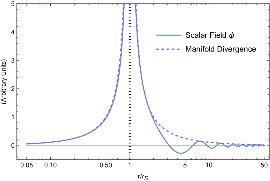
Figure 3: Radial log-linear plot of the scalar field solutions (blue solid) with the manifold divergence (purple dashed) as $(g^{11}-1)$ via Eq. (3), along the equatorial plane at $\theta=\pi/2$. The wider, black dashed line marks the event horizon, separating the interior region from the exterior region.

Figure 3 reveals that the manifold divergence aligns with the scalar field’s amplitude envelope, suggesting the scalar field kinematically traces the geometry, more for the case of the exterior. This alignment hints at possible quantum emergences from the spacetime manifold, which is akin to the vacuum Casimir effect. Unlike these emergences from a canonically flat spacetime, this emerges from a curved spacetime, although with approximated solutions rather than exact.

4.2 Mass Shell Free-fall Model

Another topic of discussion is describing BH evaporation as a mass shell free-fall model. This analysis is intentionally brief, serving as a proof of consistency rather than a novel finding. In stellar collapse, mass shell free-fall models capture surface contraction when gravitational forces overcome the nuclear pressure counter-balance. This is described by the following differential equation:

$$-\frac{1}{4\pi r^{2}}\frac{\partial^{2}r}{\partial t^{2}}=-\frac{\partial P}{\partial M}-\frac{GM}{4\pi r^{4}},$$ (44)

where $r$ is the changing radius, the left-hand side represents radially inward acceleration, $\partial P/\partial M$ is the pressure gradient with respect to mass, and $GM/(4\pi r^{4})$ is the gravitational force per unit area. For $\partial^{2}r/\partial t^{2}=0$, the inward gravitational pull is balanced by the outward nuclear pressure.

In our holographic model, the fermionic medium below the BH horizon yields a non-zero pressure $P=\rho/9=M/(12\pi r^{3})$, with $\partial P/\partial M=(12\pi r^{3})^{-1}$. This pressure provides the outward force against gravitational collapse, yet the horizon contracts due to BH evaporation driven by Hawking radiation. Timelike Hawking particles, with effective mass $m_{H}=\hbar/(4\pi GM)$ [31], excert a force equal but opposite to free-fall: $F=\hbar/(16\pi G^{2}M^{2})$ [26]. To model this as a constant free-fall rate, we equate the radial acceleration to the Hawking force per unit mass, scaled by another fine-tuning factor $\mathtt{j}$:

$$-\frac{\mathtt{j}}{4\pi r^{2}}\frac{F}{m_{H}}=-\frac{\partial P}{\partial M}-\frac{GM}{4\pi r^{4}}.$$ (45)

The non-zero pressure gradient, a hallmark of the holographic fermionic medium, disrupts the direct balance between $F/m_{H}=(4GM)^{-1}$ and the combined right-hand side terms. Without $\mathtt{j}$ in Eq. (45), the model fails to recover the Schwarzschild radius as the onset for BH evaporation, while it is otherwise retrievable with a zero pressure gradient and omitting $\mathtt{j}$. Thus, $\mathtt{j}$ is a necessary ad hoc correction, acting as a holographic enhancer to calibrate the force and account for the medium’s pressure, with its value determined algebraically.

Since the BH radius scales with mass, we derive $\mathtt{j}$ using a thoroughly radius-dependent form of Eq. (45), with $F/m_{H}=1/(2r)$:

$$\frac{\mathtt{j}}{8\pi r^{3}}=\frac{1}{12\pi r^{3}}+\frac{1}{8\pi r^{3}},$$ (46)

which solves for the fine-tuning parameter $\mathtt{j}$ algebraically as the value 5/3. The same value for j is recovered if a throughly mass-dependent form was considered. For constant mass shell free-fall at the inital BH mass $M=M_{0}$, and using $\mathtt{j}=5/3$, the BH horizon free-fall model reads:

$$\frac{5}{12GM_{0}}=\frac{1}{3r}+\frac{GM_{0}}{r^{2}},$$ (47)

which presents itself as a quadratic polynomial in $u=1/r$. Solving for the zeroes of $u$ retieves respective minimum values (i.e., respective maximum values of $r$) where BH horizon free-fall begins. Via the quadratic formula for $u$, the positive zero value recovers the Schwarzschild radius:

$$u_{0}=\frac{1}{2GM_{0}}\implies r_{0}=2GM_{0}.$$ (48)

This confirms that BH horizon contraction via Hawking radiation begins at the initial Schwarzschild radius. Furthermore, this validates the fermionic medium’s compatibility with standard evaporation dynamics. The parameter $\mathtt{j}$ ensures this consistency, although its ad hoc nature suggests future work to derive it from first principles. Further studies could explore how the medium’s neutrino-dominated degeneracy affects emission rates (i.e., BH lifespans) or back-reaction effects.

5 Conclusion

This study models a Schwarzschild black hole as a holographic medium with fermionic degrees of freedom, offering a novel perspective on its geometry and dynamics. The Schwarzschild spacetime incorporates a black 2-brane on $n=4$ physical dimensions as its spherical boundary, revising the metric such that the BH horizon is the region of attraction for exterior, interior, and co-moving observers. Dynamically, infalling objects and internal holographic particles are drawn to this boundary, preserving the external perception of suspended animation and suggesting that Hawking radiation represents the ejection of conserved information from prior infalling matter.

Using the Einstein-Hilbert action with a Gibbons-Hawking-York boundary term, we derive a Lagrangian with the 4D Ricci scalar as the kinetic driver and the square of extrinsic curvature as the potential gauge. The resulting Hamiltonian yields a Schrödinger-like equation, resembling the contracted Einstein field equations, which provides a quantum-like framework for the manifold’s dynamics. For a traceless perfect fluid, hydrodynamic insights emerge through an equation of state (Eq. [25]) and the Fermi energy, quantifying the holographic medium’s degeneracy. The mass shell free-fall model verifies that the horizon’s contraction during evaporation begins at the initial Schwarzschild radius, consistent with general relativity, while spherical wave solutions to the Schrödinger-like equation describe emergent fluctuations of the manifold.

This holographic model advances our understanding of BH interiors by unifying quantum and gravitational effects, with the fermionic medium offering a potential resolution to the information paradox. However, the reliance on fine-tuning parameters (e.g. $\mathtt{a}=1/12$ and $\mathtt{j}=5/3$) highlights the model’s preliminary nature, necessitating future work to derive these from first principles rather than from ad hoc assertions. Further studies could explore the neutrino-dominated medium’s impact on evaporation rates, back-reaction effects, or observational signatures like gravitational wave signals and x-ray emission bursts [33]. By providing a consistent framework that bridges classical and quantum regimes, this study lays a foundation for deeper investigations into the holographic nature of BHs and the fundamental structure of quantum gravity.

Acknowledgments

A holographic model for Schwarzschild BHs is thanks to productive discussions with Percy Martinez.

References

- [1] K. Schwarzschild, Sitzungsber. Preuss. Akad. Wiss. Berlin (Math. Phys. ) 1916, 189-196 (1916) [arXiv:physics/9905030 [physics]].
- [2] K. Schwarzschild, Sitzungsber. Preuss. Akad. Wiss. Berlin (Math. Phys. ) 1916, 424-434 (1916) [arXiv:physics/9912033 [physics.hist-ph]].
- [3] R. Penrose, Phys. Rev. Lett. 14, 57-59 (1965) doi:10.1103/PhysRevLett.14.57
- [4] S. W. Hawking, Nature 248, 30-31 (1974) doi:10.1038/248030a0
- [5] S. W. Hawking, Commun. Math. Phys. 43, 199-220 (1975) [erratum: Commun. Math. Phys. 46, 206 (1976)] doi:10.1007/BF02345020
- [6] J. W. York, Jr., Phys. Rev. Lett. 28, 1082-1085 (1972) doi:10.1103/PhysRevLett.28.1082
- [7] G. W. Gibbons and S. W. Hawking, Phys. Rev. D 15, 2752-2756 (1977) doi:10.1103/PhysRevD.15.2752
- [8] P. Kovtun, D. T. Son and A. O. Starinets, Phys. Rev. Lett. 94, 111601 (2005) doi:10.1103/PhysRevLett.94.111601 [arXiv:hep-th/0405231 [hep-th]].
- [9] O. Lunin and S. D. Mathur, Nucl. Phys. B 623, 342-394 (2002) doi:10.1016/S0550-3213(01)00620-4 [arXiv:hep-th/0109154 [hep-th]].
- [10] O. Lunin and S. D. Mathur, Phys. Rev. Lett. 88, 211303 (2002) doi:10.1103/PhysRevLett.88.211303 [arXiv:hep-th/0202072 [hep-th]].
- [11] S. D. Mathur, Int. J. Mod. Phys. D 11, 1537-1540 (2002) doi:10.1142/S0218271802002852 [arXiv:hep-th/0205192 [hep-th]].
- [12] S. D. Mathur, Fortsch. Phys. 53, 793-827 (2005) doi:10.1002/prop.200410203 [arXiv:hep-th/0502050 [hep-th]].
- [13] S. D. Mathur, Lect. Notes Phys. 769, 3-48 (2009) doi:10.1007/978-3-540-88460-6_1 [arXiv:0803.2030 [hep-th]].
- [14] S. D. Mathur, [arXiv:0810.4525 [hep-th]].
- [15] S. D. Mathur, Class. Quant. Grav. 26, 224001 (2009) doi:10.1088/0264-9381/26/22/224001 [arXiv:0909.1038 [hep-th]].
- [16] S. D. Mathur, Annals Phys. 327, 2760-2793 (2012) doi:10.1016/j.aop.2012.05.001 [arXiv:1205.0776 [hep-th]].
- [17] F. R. Tangherlini, Nuovo Cim. 27, 636-651 (1963) doi:10.1007/BF02784569
- [18] N. A. Obers, Lect. Notes Phys. 769, 211-258 (2009) doi:10.1007/978-3-540-88460-6_6 [arXiv:0802.0519 [hep-th]].
- [19] G. Dvali and C. Gomez, Fortsch. Phys. 61, 742-767 (2013) doi:10.1002/prop.201300001 [arXiv:1112.3359 [hep-th]].
- [20] G. Dvali and C. Gomez, Phys. Lett. B 716, 240-242 (2012) doi:10.1016/j.physletb.2012.08.019 [arXiv:1203.3372 [hep-th]].
- [21] G. Dvali and C. Gomez, Phys. Lett. B 719, 419-423 (2013) doi:10.1016/j.physletb.2013.01.020 [arXiv:1203.6575 [hep-th]].
- [22] G. Dvali and C. Gomez, Eur. Phys. J. C 74, 2752 (2014) doi:10.1140/epjc/s10052-014-2752-3
- [23] S. K. Manikandan and A. N. Jordan, Phys. Rev. D 98, no.12, 124043 (2018) doi:10.1103/PhysRevD.98.124043 [arXiv:1811.03209 [gr-qc]].
- [24] P. Hayden and J. Preskill, JHEP 09, 120 (2007) doi:10.1088/1126-6708/2007/09/120 [arXiv:0708.4025 [hep-th]].
- [25] D. N. Page, Phys. Rev. D 13, 198-206 (1976) doi:10.1103/PhysRevD.13.198
- [26] N. M. MacKay, [arXiv:2503.18086 [gr-qc]].
- [27] R. L. Arnowitt, S. Deser and C. W. Misner, Phys. Rev. 116, 1322-1330 (1959) doi:10.1103/PhysRev.116.1322
- [28] B. Chow, D. Knopf. The Ricci Flow: An Introduction (Providence, R.I.: American Mathematical Society, 2004) ISBN 0-8218-3515-7.
- [29] B. Li, [arXiv:2411.15164 [physics.gen-ph]].
- [30] H. Wang and J. Wang, Adv. High Energy Phys. 2020, 9102461 (2020) doi:10.1155/2020/9102461 [arXiv:2006.00433 [hep-th]].
- [31] N. M. MacKay, [arXiv:2502.08816 [gr-qc]].
- [32] N. D. Birrell and P. C. W. Davies, Cambridge University Press, 1982, ISBN 978-0-511-62263-2, 978-0-521-27858-4 doi:10.1017/CBO9780511622632
- [33] P. Bak. “Earthquakes, Starquakes, and Solar Flares.” In: How Nature Works (New York, N.Y.: Copernicus, 1996) doi:10.1007/978-1-4757-5426-1_5