Quantum Annealing Algorithms for Estimating Ising Partition Functions

Abstract

Estimating partition functions of Ising spin glasses is crucial in statistical physics, optimization, and machine learning, yet remains classically intractable due to its $\#$P-hard complexity. While Jarzynski’s equality offers a theoretical approach, it becomes unreliable at low temperatures due to rare divergent statistical fluctuations. Here, we present a protocol that overcomes this limitation by synergizing reverse quantum annealing with tailored nonequilibrium initial distributions. Our method can dramatically suppress the estimator variance, achieving saturation in the low-temperature regime. Numerical benchmarks on the Sherrington–Kirkpatrick spin glass and the 3-SAT problem demonstrate that our protocol reduces scaling exponents by over an order of magnitude (e.g., from $\sim 8.5$ to $\sim 0.5$), despite retaining exponential system-size dependences. Crucially, our protocol circumvents stringent adiabatic constraints, making it feasible for near-term quantum devices like superconducting qubits, trapped ions, and Rydberg atom arrays. This work bridges quantum dynamics with computational complexity, offering a practical pathway to quantum advantage in spin glass thermodynamics and beyond.

Introduction.— Ising spin glasses (ISGs) play a pivotal role in both fundamental research and practical applications across diverse disciplines [1, 2, 3, 4], including statistical physics [5], combinatorial optimization [6], and machine learning [7]. Despite its broad relevance, a longstanding challenge persists: estimating the Ising partition functions (IPFs) of these complex systems [8], which is classically intractable, being $\#$P-hard in the worst case [9]. In view of this fundamental barrier, quantum algorithms have emerged as promising candidates for circumventing classical limitations. Recent proposals include quantum circuit mappings [10, 11, 12], dynamical quantum simulators [13], and DQC1-based algorithms [14]. However, these methods are restricted to idealized settings. The critical challenge lies in achieving practical quantum advantage on current noisy intermediate-scale quantum (NISQ) hardwares [15].

Here, we address this challenge directly by harnessing quantum annealing (QA) processors. QA has the potential to revolutionize complex optimization problems and thereby impact science and numerous real-world applications [16, 17, 18, 19, 20, 21]. QA offer a provable quantum scaling speedup for identifying the ground states of ISGs [19, 20, 21], which is known to be NP-hard for classical computers [22]. To achieve this advantage, tremendous efforts have been devoted to developing QA hardwares [23], such as superconducting qubits [24, 25], trapped ions [26, 27], and Rydberg atom arrays [28, 29]. Recent breakthroughs extend QA’s utility beyond the ground-state search. For instance, QA-enabled Gibbs sampling [30, 31, 32] has demonstrated success in approximating the finite-temperature properties of ISGs. These advances collectively position QA as a versatile quantum tool for estimating IPFs.

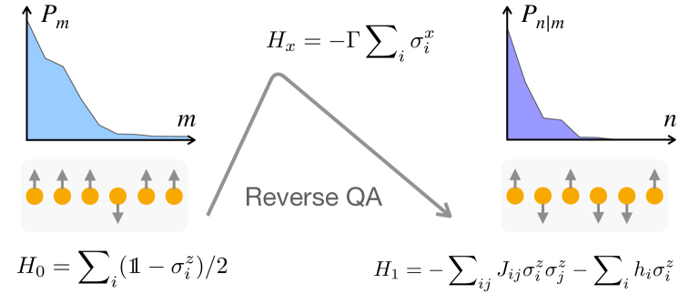
Figure 1: Schematics of our protocol for estimating IPFs. The protocol begins by preparing the system in an initial state sampled from a distribution $P_{m}$. Unlike conventional JE approaches that assume thermal equilibrium (e.g., Gibbs distributions), $P_{m}$ is intentionally designed to deviate from equilibrium to suppress the variance. The system then goes through a nonequilibrium reverse QA process [Eq. (1)], in which the Hamiltonian transitions from a trivial free model $H_{0}$ to the desired target ISG $H_{1}$ with the aid of a driver $H_{x}$. Finally, projective measurements in the eigenbasis of $H_{1}$ yield outcomes governed by the conditional probability $P_{n|m}$ [see details above Eq. (2)]. These outcomes are processed via the estimator to reconstruct the IPFs of $H_{1}$ [Eq. (3)].

In this work, we present a quantum protocol for estimating IPFs leveraging reverse QA architectures [33, 34, 35, 36, 37]. Inspired by Jarzynski’s equality (JE) [38, 39, 40, 41]—a cornerstone of fluctuation relations connecting thermodynamics with nonequilibrium fluctuations [42, 43]—our protocol bypasses key limitations of conventional JE-based approaches. While JE links equilibrium partition functions to nonequilibrium work averages via $\left\langle\exp(-\beta W)\right\rangle=Z_{1}(\beta)/Z_{0}(\beta)$, where $Z_{0}(\beta)$ and $Z_{1}(\beta)$ are partition functions of the initial/target Hamiltonian, respectively [see details below Eq. (2)], its practical utility is crippled at low temperatures by rare events dominating the exponential average [44]. Existing mitigation strategies, such as those based on adiabaticity or shortcuts [45, 46], demand impractically long coherence time or control complexity. In contrast, in the following, we discuss a completely distinctive scheme (Fig. 1), in which we replace the conventional Gibbs initial state with a well-designed nonequilibrium one, dramatically reducing estimator variance. The ISG Hamiltonian $H_{1}$ is reached via a reverse QA path [Eq. (1)], evolving from a simple $H_{0}$ with the aid of a driver $H_{x}$. This minimizes quantum resource demands while suppressing work fluctuations. Unlike JE, where variance grows exponentially as the temperature approaches zero, our protocol achieves saturation at low temperatures [Fig. 3 (a1, b1)]. Despite the exponential system-size scaling of variances, our method outperforms JE by orders of magnitude at low temperatures [Fig. 3 (a2, b2)]. Besides, our protocol avoids adiabatic constraints, enabling execution on NISQ devices with finite coherence times [Fig. 3 (a3, b3)]. By exploiting quantum dynamics to sidestep rare-event bottlenecks, our protocol establishes quantum processors as a transformative platform for ISG studies. This work advances applications in ISG physics, optimization, and machine learning, where IPFs estimation is critical yet classically intractable.

Reverse quantum annealing protocol.— Reverse QA enables state-selective initialization of QA dynamics—a feature critical for applications such as hybrid quantum-classical optimization [34] and quantum simulations [35]. The reverse QA protocol can be described by the following form of a time-dependent Hamiltonian [36, 37]

$$H(t)=s(t)H_{1}\, +\,[1-s(t)]\lambda(t)H_{x}$$ (1)

$$+\,[1-s(t)][1-\lambda(t)]H_{0}\,.$$

Here, the time-dependent parameters $s(t)$ and $\lambda(t)$ both grow from $0$ to $1$ over the course of the unitary time evolution $U(\tau)=\mathcal{T}\exp[-i\int_{0}^{\tau}H(t)\,{\rm d}t]$ with $\tau$ the total time and $\mathcal{T}$ the time-ordering operator. The system thus transitions from the initial Hamiltonian $H_{0}$ to the target Hamiltonian $H_{1}$, aided by the driver Hamiltonian $H_{x}$. In our context of the ISG problem, $H_{0}=\sum_{i=1}^{N}({\openone}-\sigma^{z}_{i})/2$, $H_{1}=-\sum^{N}_{i,j=1}J_{ij}\sigma^{z}_{i}\sigma^{z}_{j}-\sum^{N}_{i=1}h_{i}\sigma^{z}_{i}$, and $H_{x}=-\Gamma\sum^{N}_{i=1}\sigma^{x}_{i}$ where ${\openone}$ is the identity operator, $\{\sigma^{x/z}_{i}\}$ are the Pauli-$x/z$ operators, and $N$ is the system size. The spin-spin couplings $J_{ij}$ and the local fields $h_{i}$ defines a model instance [19, 20], and $\Gamma$ sets the scale of quantum fluctuations for state transitions. Hereafter, we set $\hbar=1$ and $k_{\rm B}=1$, use $\Gamma$ as our energy unit, and choose $s(t)=\lambda(t)=t/\tau$.

Let $\{E^{0}_{m},\,\left|\psi^{0}_{m}\right\rangle\}$ and $\{E^{1}_{n},\,\left|\psi^{1}_{n}\right\rangle\}$ denote the ascending eigenvalues and corresponding eigenstates of $H_{0}$ and $H_{1}$, respectively. The system is initialized by randomly sampling $\left|\psi^{0}_{m}\right\rangle$ according to a sampling function $P_{m}$, which satisfies $P_{m}>0$ and $\sum^{D}_{m=1}P_{m}=1$ with $D=2^{N}$ the dimension of the Hilbert space. Under the reverse QA dynamics, the initial state evolves to $\left|\psi(\tau)\right\rangle=U(\tau)\left|\psi^{0}_{m}\right\rangle$. The following projective measurement in the eigenbasis of $H_{1}$ yields a trajectory $\left|\psi^{0}_{m}\right\rangle\to\left|\psi^{1}_{n}\right\rangle$ with a conditional probability $P_{n|m}={\left|\left\langle\psi^{1}_{n}\right|U(\tau)\left|\psi^{0}_{m}\right\rangle\right|}^{2}$. Due to the unitarity of $U(\tau)$, we have $\sum^{D}_{m=1}P_{n|m}=1$. Now we are ready to reconstruct the IPFs of $H_{1}$ as

$$Z_{1}(\beta) = \sum\nolimits^{D}_{n=1}\exp\left(-\beta E^{1}_{n}\right)$$ (2)

$$= \sum\nolimits^{D}_{m,n=1}\frac{\exp\left(-\beta E^{1}_{n}\right)}{P_{m}}P_{n|m}P_{m}\,,$$

where $\beta=1/T$ is the inverse temperature. This estimator leverages correlations between initial ($P_{m}$) and transition ($P_{n|m}$) probabilities to bypass direct summation over $D$ states.

Note that choosing $P_{m}=P^{\rm G}_{m}(\beta)\equiv\exp(-\beta E^{0}_{m})/Z_{0}(\beta)$ (Gibbs distribution) will reduce Eq. (2) to the celebrated JE: $Z_{1}(\beta)/Z_{0}(\beta)=\exp(-\beta\Delta F)=\left\langle\exp(-\beta W)\right\rangle$ [38, 39, 40, 41]. Here, $Z_{0}(\beta)=[1+\exp(-\beta)]^{N}$ is the trivial partition function of $H_{0}$, $\Delta F=-\beta^{-1}\log[Z_{1}(\beta)/Z_{0}(\beta)]$ is the free energy difference, and the expectation value $\left\langle\exp(-\beta W)\right\rangle=\sum^{D}_{m,n=1}\exp(-\beta W_{nm})P_{n|m}P_{m}$ with $W_{nm}=E^{1}_{n}-E^{0}_{m}$ the quantum work defined through a two-point measurement scheme [39, 40, 41]. By enabling efficient preparation of initial Gibbs ensembles, this protocol establishes quantum processors as practical tools for ISG thermodynamics—directly supporting applications such as validating fluctuation theorems in many-body regimes [47] and efficient free-energy computation for disordered systems [48].

In the following, we focus on estimating the IPFs of $H_{1}$ based on Eq. (2), to achieve contrasted protocol advantages over conventional JE-based approaches. To demonstrate the efficiency of our protocol, we benchmark it against two canonical ISG models: the Sherrington–Kirkpatrick (SK) spin glass [49, 50] and the random 3-SAT [51]. The Hamiltonian of the SK model reads $H_{\rm SK}=\frac{1}{\sqrt{N}}\sum^{N}_{(j\neq i)=1}J_{ij}\sigma^{z}_{i}\sigma^{z}_{j}+\sum^{N}_{i=1}h_{i}\sigma^{z}_{i}\,,$ where $J_{ij}$ and $h_{i}$ are independent variables sampled from the standard normal distribution. And the random 3-SAT is a fundamental Boolean satisfiability problem. The hard instances are generated via a physics-inspired protocol with planted solutions, ensuring controlled benchmarking in classically intractable regimes [52].

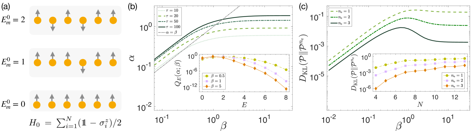
Figure 2: Approximation strategies for optimized sampling functions in the SK spin-glass model. (a) Initial spin configurations. Arrows represent spins in the eigenstates of $\sigma^{z}$, $\{\left|\uparrow\right\rangle,\left|\downarrow\right\rangle\}$ (eigenvalues $+1$ and $-1$, respectively). The initial product state $\left|\psi^{0}_{m}\right\rangle=\otimes^{N}_{i=1}\left|\gamma_{i}\right\rangle$ ($\left|\gamma_{i}\right\rangle\in\{\left|\uparrow\right\rangle,\left|\downarrow\right\rangle\}$), is an eigenstate of $H_{0}$. The number of $\left|\downarrow\right\rangle$ in $\left|\psi^{0}_{m}\right\rangle$ equals its energy $E^{0}_{m}$, with $I_{E}=\{m|E^{0}_{m}=E\}$ indexing degenerate states of energy $E$. (b) Gibbs approximation of $\mathcal{P}_{m}(\beta)$. The optimized sampling function $\mathcal{P}_{m}(\beta)$ is approximated by a Gibbs distribution $P^{G}_{m}(\alpha)$ for total evolution times $\tau=10,20,50,100$. The gray dashed-dotted $\alpha=\beta$ line is drawn for reference purposes. The inset shows the distribution $Q_{E}(\alpha,\beta)$ for $\beta=0.5,1,5$ with $\tau=100$. Here, we have chosen the system size $N=8$. (c) Perturbative approximation of $\mathcal{P}_{m}(\beta)$. The Kullback–Leibler divergence $D_{\rm KL}(\mathcal{P}\|\mathcal{P}^{n_{\rm e}})=\sum_{m}\mathcal{P}_{m}\log(\mathcal{P}_{m}/\mathcal{P}^{n_{\rm e}}_{m})$ [53] quantifies the difference between $\mathcal{P}_{m}(\beta)$ and $\mathcal{P}^{n_{\rm e}}_{m}(\beta)$ for $n_{\rm e}=1,2,3$. Main panel: $\beta$-dependence ($N=8$, $\tau=100$). Inset: System-size scaling ($N=4\text{--}13$, $\tau=100$, $\beta=10$). All data are averaged over $10^{3}$ Hamiltonian instances.

Optimized sampling function.— In practice, however, the convergence of the JE estimator is notoriously slow [44, 45]. This arises because the work distribution exhibits a large variance, and rare but critical negative $W$ trajectories—essential for accurate estimation—are statistically underrepresented with finite samplings. To address this, we propose replacing the conventional Gibbs distribution with a tailored nonequilibrium one. As shown below, this approach dramatically suppresses estimator variance, especially in the low-temperature regime.

From Eq. (2), the IPFs of $H_{1}$ can be estimated as

$$Z_{1}(\beta)=\left\langle z_{m,n}(\beta)\right\rangle\approx Z_{\rm est}(\beta)\equiv\frac{1}{M_{\rm s}}\sum z_{m,n}(\beta)\,,$$ (3)

where $\left\langle\cdot\right\rangle$ denotes averaging over trajectories $\left|\psi^{0}_{m}\right\rangle\to\left|\psi^{1}_{n}\right\rangle$ sampled with $P_{n|m}P_{m}$, $z_{m,n}(\beta)=\exp(-\beta E^{1}_{n})/P_{m}$ is the corresponding random variable, and $M_{\rm s}$ is the total sample number. While the equality holds exactly as $M_{\rm s}\to\infty$, finite sampling necessitates clever design of the initial distribution $P_{m}$ and transition probability $P_{n|m}$ to minimize estimator variance. Our protocol thus operates as a hybrid classical-quantum algorithm, i.e., the initial state is randomly chosen from $P_{m}$, a classical distribution designed to minimize statistical fluctuations in $Z_{\rm est}$; the transition $\left|\psi^{0}_{m}\right\rangle\to\left|\psi^{1}_{n}\right\rangle$ is governed by $P_{n|m}$, implemented via quantum dynamics (e.g., reverse QA). For the latter, it is known that increasing the evolution time $\tau$ can reduce the required $M_{\rm s}$ [54]. However, practical limitations—notably finite coherence time in quantum hardwares—constrain $\tau$, demanding a balance between quantum resource allocation and sampling efficiency. This raises a central question for reverse QA with finite $\tau$: What choice of $P_{m}$ minimizes the variance of $Z_{\rm est}$ for a given reverse QA protocol?

To address this problem, we examine the variance of the estimator $z_{m,n}(\beta)$, defined as [52]

$$\sigma^{2}(\beta) = \sum\nolimits^{D}_{m,n=1}\left[z_{m,n}(\beta)-Z_{1}(\beta)\right]^{2}P_{n|m}P_{m}$$ (4)

$$= \sum\nolimits^{D}_{m=1}\frac{\mu_{m}(\beta)}{P_{m}}-Z^{2}_{1}(\beta)\,.$$

Here, $\mu_{m}(\beta)=\sum^{D}_{n=1}\exp(-2\beta E^{1}_{n})P_{n|m}$. Guided by importance sampling principles [55], we seek to minimize $\sigma^{2}(\beta)$ by optimizing $P_{m}$. A direct constrained minimization yields the theoretically optimal distribution $P_{m}=\mathcal{P}_{m}(\beta)\equiv\sqrt{\mu_{m}(\beta)}/\mathcal{N}_{\mathcal{P}}(\beta)$, where $\mathcal{N}_{\mathcal{P}}(\beta)$ ensures normalization [52]. While $\mathcal{P}_{m}(\beta)$ guarantees the minimal variance, its direct computation is infeasible for finite $\tau$ in practical implementations. To resolve this, we develop an efficient approximation scheme for $\mathcal{P}_{m}(\beta)$ as follows.

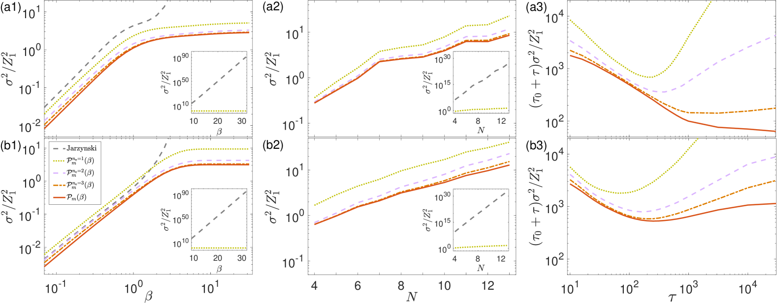
Figure 3: Performance evaluation of our protocol for the SK spin-glass (a1-a3) and 3-SAT (b1-b3) models. The red solid line indicates the optimal sampling function $\mathcal{P}_{m}(\beta)$. And the approximations $\mathcal{P}^{n_{\rm e}}_{m}(\beta)$ for $n_{\rm e}=1,2,3$ are depicted as follows: $n_{\rm e}=1$ (light green dotted line), $n_{\rm e}=2$ (purple dashed line), and $n_{\rm e}=3$ (orange dash-dotted line). Results from the JE-based approach (gray dashed line) are included for comparison. Here, we have chosen the system size $N=8$ for (a1, b1, a3, b3), the inverse temperature $\beta=10$ for (a2, b2, a3, b3), and the initialization and measurement time $\tau_{0}=100$ for (a3, b3). All data are averaged over $10^{3}$ Hamiltonian instances.

The simplest approximation replaces $\mathcal{P}_{m}(\beta)$ with a Gibbs distribution $P^{\rm G}_{m}(\alpha)$, parameterized by a variational inverse temperature $\alpha$. For a fixed $\beta$, we optimize $\alpha$ to minimize $\sigma^{2}(\beta)$. This reduces to solving the minimization problem $\min_{\alpha}\sum^{D}_{m=1}\mu_{m}(\beta)/P^{\rm G}_{m}(\alpha)$, and from which we identify the unique optimal $\alpha$ that satisfies [52]

$$\frac{N}{1+\exp(\alpha)}=\sum\nolimits^{N}_{E=0}E\cdot Q_{E}(\alpha;\beta)\,.$$ (5)

Here, $Q_{E}(\alpha;\beta)\propto\exp(\alpha E)\sum_{m\in I(E)}\mu_{m}(\beta)$ is a distribution, and $I_{E}=\{m|E^{0}_{m}=E\}$ groups degenerate initial states $\left|\psi^{0}_{m}\right\rangle$ sharing the same energy $E$ [Fig. 2 (a)]. Numerical results for the SK spin glass [Fig. 2 (b)] reveal two key features: (i) As $\beta$ increases, $\alpha$ rises initially before saturating to a $\tau$-dependent value; (ii) Longer $\tau$ increases $\alpha$, concentrating $P^{\rm G}_{m}(\alpha)$ and reducing the computational effort to estimate $Z_{1}(\beta)$, which is consistent with previous works [54]. These behaviors starkly contrast with JE, which fixes $\alpha\equiv\beta$. JE’s rigidity leads to inefficient sampling in low temperatures, as high-energy states are inadequately probed. Similar trends have been observed in other complex systems, such as the 3-SAT [52], underscoring the generality of this approach.

While $P^{\rm G}_{m}(\alpha)$ outperforms $P^{\rm G}_{m}(\beta)$, determining $\alpha$ via Eq. (5) for large system sizes remains challenging. This issue can be mitigated based on three key observations. Firstly, $P^{\rm G}_{m}(\alpha)$, while simpler, reasonably approximates the optimal distribution $\mathcal{P}_{m}(\beta)\propto\sqrt{\mu_{m}(\beta)}$ [52]. Its defining property, $P^{\rm G}_{m\in I_{E+1}}(\alpha)=\exp(-\alpha)P^{\rm G}_{m\in I_{E}}(\alpha)$, leads to the approximation

$$\bar{\nu}_{E+1}(\beta)\approx\exp(-\alpha)\bar{\nu}_{E}(\beta)\,,$$ (6)

where $\bar{\nu}_{E}(\beta)=\sum_{m\in I_{E}}\sqrt{\mu_{m}(\beta)}/\binom{N}{E}$ averages $\sqrt{\mu_{m}(\beta)}$ over the $E^{0}_{m}=E$ degenerate subspace. Secondly, combining Eq. (6) and the definition of $Q_{E}$, we find that $Q_{E}$ decays exponentially with large $E$ [see Fig. 2 (b), inset]. Consequently, only contributions from low-energy subspaces ($E\ll N$) significantly affect the expectation value on the RHS of Eq. (5). Thirdly, for low-energy initial states ($m\in I_{E}$, $E\ll N$), we compute $\mu_{m}(\beta)=\sum^{D}_{n=1}\exp(-2\beta E^{1}_{n})P_{n|m}$ using experimentally sampled trajectories $\left|\psi^{0}_{m}\right\rangle\to\left|\psi^{1}_{n}\right\rangle$ [52]. Crucially, these trajectories are reused to calculate $Z_{1}(\beta)$ after determining the sampling function $P_{m}$, incurring negligible additional computational costs.

Guided by these findings, we propose a family of sampling functions $\mathcal{P}^{n_{\rm e}}_{m}(\beta)\,(n_{\rm e}=1,2,\dots,N)$ to approximate $\mathcal{P}_{m}(\beta)$. The construction involves four main steps as detailed in the Supplemental Material [52]. Firstly, we introduce the auxiliary variables $\{\nu_{m}(\beta)\}|_{m=1,2,\dots,D}$ and set $\nu_{m}(\beta)=\sqrt{\mu_{m}(\beta)}$ for $m\in I_{E\leq n_{\rm e}}$. These $\mu_{m}(\beta)$ can be obtained experimentally via trajectory sampling as mentioned earlier. Secondly, for $m\in I_{E>n_{\rm e}}$, we iteratively construct $\nu_{m}(\beta)$ via the ansatz

$$\nu_{m\in I_{E+1}}(\beta)=\frac{\exp(-\alpha)}{E+1}\sum\nolimits_{m^{\prime}\in J_{E}(m)}\nu_{m^{\prime}}(\beta)\,,$$ (7)

where $\alpha$ is a parameter determined self-consistently, $J_{E}(m)=\{m^{\prime}|m^{\prime}\in I_{E}\,,m\in I_{E+1}\,,D_{\rm H}(m^{\prime},m)=1\}$ contains states $m^{\prime}\in I_{E}$ adjacent to $m$. Here, $D_{\rm H}(m^{\prime},m)$ is the Hamming distance (i.e., the number of different spins) between $\left|\psi^{0}_{m^{\prime}}\right\rangle$ and $\left|\psi^{0}_{m}\right\rangle$ [Fig. 2 (a)]. This ensures consistency with the exponential decay relation in Eq. (6). Thirdly, we approximate $\mu_{m}(\beta)\approx\nu^{2}_{m}(\beta)$ for $m\in I_{E>n_{\rm e}}$. Substituting all $\mu_{m}(\beta)$ into Eq. (5) yields a closed-form solution for $\alpha$ . Finally, the $n_{\rm e}$-th order approximation is given by $\mathcal{P}^{n_{\rm e}}_{m}(\beta)\propto\nu_{m}(\beta)$, normalized over all $m$. As shown in Fig. 2 (c), we find that increasing $n_{\rm e}$ significantly improves fidelity of $\mathcal{P}_{m}(\beta)$, particularly at low temperatures. Besides, the approximation remains robust as system size $N$ grows [Fig. 2 (c), inset], with significant error reduction even for modest $n_{\rm e}$.

Results.— To assess the efficacy of our protocol, we employ the estimator variance $\sigma^{2}$ as the performance metric. Numerical results for the SK spin glass and 3-SAT models are presented in Fig. 3. Both systems demonstrate that our protocol is superior to the JE-based approach. Notably, in the low-temperature regime, the variance of our protocol—even when using the simplified sampling function $\mathcal{P}^{n_{\rm e}=1}_{m}(\beta)$—saturates, whereas the JE-based method exhibits exponential divergence [Fig. 3 (a1, b1), insets]. Given that estimating IPFs is $\#$P-hard, quantum computers cannot reasonably be expected to solve this task in polynomial time. To quantify performance under this fundamental restriction, we analyze the scaling of $\sigma^{2}/Z^{2}_{1}\sim D^{\gamma}$ at a representative low temperature [$\beta=10$, see insets of Fig. 3 (a2, b2)], and extract the following exponents: (i) SK spin glass: $\gamma_{1}=0.446$ vs. $\gamma_{2}=6.993$; (ii) 3-SAT: $\gamma_{1}=0.502$ vs. $\gamma_{2}=8.451$. Here, $\gamma_{1}$ and $\gamma_{2}$ are the exponents of our protocol with $\mathcal{P}^{n_{\rm e}=1}_{m}(\beta)$ as the sampling function and the JE-based approach, respectively. These results demonstrate that, despite its exponential scaling of variance with system size, our protocol outperforms the JE-based method by orders of magnitude in the low-temperature regime. A full complexity analysis of the scaling properties of $\mathcal{P}_{m}(\beta)$ further corroborates these results [52].

Furthermore, because the number of samples needed to suppress estimation errors scales with the variance, we define the total resource cost as $\mathcal{M}_{\rm s}=(\tau_{0}+\tau)\sigma^{2}$, where $\tau_{0}$ denotes the initialization and measurement time per sample. While $\sigma^{2}$ decreases with increasing total evolution time $\tau$, the trade-off between $\tau$ and $\sigma^{2}$ leads to an optimal finite $\tau$ that minimizes $\mathcal{M}_{\rm s}$. This implies that the most efficient protocol operates at a non-adiabatic evolution time, making it feasible for implementation on NISQ devices with limited coherence times. Empirical validation of this finding is provided in Fig. 3 (a3, b3).

Conclusion and discussion.— We have presented an efficient QA-inspired protocol for estimating IPFs, circumventing the fundamental limitations of conventional JE-based approaches. By leveraging reverse QA to evolve from a trivial initial Hamiltonian to the target ISG, and optimizing initial distributions to minimize variance, we sidestep the rare-event bottleneck inherent in the JE. Our results highlight the potential of nonequilibrium quantum dynamics to tackle classically intractable problems in ISGs. The protocol’s compatibility with NISQ-era devices [24, 25, 26, 27, 28, 29] positions it as a timely contribution to the growing toolkit of quantum-enhanced algorithms, offering a blueprint for leveraging quantum fluctuations and tailored sampling to overcome classical limitations. As quantum hardwares mature, such strategies could unlock new insights into complex energy landscapes, from protein folding [56] to machine learning [57], bridging the gap between theoretical quantum advantage and impactful applications.