Differentially Private Secure Multiplication with Erasures and Adversaries

Abstract

We consider a private distributed multiplication problem involving $\mathsf{N}$ computation nodes and $\mathsf{T}$ colluding nodes. Shamir’s secret sharing algorithm provides perfect information-theoretic privacy, while requiring an honest majority, i.e., $\mathsf{N}\geq 2\mathsf{T}+1$. Recent work has investigated approximate computation and characterized privacy-accuracy trade-offs for the honest minority setting $(N\leq 2\mathsf{T})$ for real-valued data, quantifying privacy leakage via the differential privacy (DP) framework and accuracy via the mean squared error. However, it does not incorporate the error correction capabilities of Shamir’s secret-sharing algorithm. This paper develops a new polynomial-based coding scheme for secure multiplication with an honest minority, and characterizes its achievable privacy-utility tradeoff, showing that the tradeoff can approach the converse bound as closely as desired. Unlike previous schemes, the proposed scheme inherits the capability of the Reed-Solomon (RS) code to tolerate erasures and adversaries. We utilize a modified Berlekamp–Welch algorithm over the real number field to detect adversarial nodes.

I Introduction

Secure multi-party computation allows multiple parties to collaboratively perform a computation over their private inputs while preserving the confidentiality of those inputs[1]. A central coding theoretic technique in this area is Shamir’s secret sharing [2], a method rooted in Reed Solomon (RS) codes [3] that provides a framework for ensuring information-theoretic privacy. Consider an $\mathsf{N}$-node secure computation system designed to compute the product of two random variables $A,B\in\mathbb{F}$, where $\mathbb{F}$ is a finite field. Let $\{R_{t},S_{t}\}_{t=1}^{\mathsf{T}}$ be independent random noise variables uniformly distributed over the field. Shamir’s secret sharing algorithm encodes $A,B$ by constructing polynomials:

$$p_{1}(x)=A+\sum_{t=1}^{\mathsf{T}}R_{t}x^{t},\quad p_{2}(x)=B+\sum_{t=1}^{\mathsf{T}}S_{t}x^{t}.$$ (1)

Node $i$ receives $p_{1}(x_{i})$ and $p_{2}(x_{i})$, where $\{x_{1},\cdots,x_{\mathsf{N}}\}$ denote non-zero distinct elements over the field $\mathbb{F}$. Any set of $\mathsf{T}$ colluding nodes fail to recover $A$ and $B$, but at least $2\mathsf{T}+1$ nodes are required to obtain the product $AB$ by interpolating the $2\mathsf{T}$-degree polynomial $p_{1}(x)p_{2}(x)$. In other words, perfect information-theoretic privacy requires an honest majority to ensure security and correctness. Secure computation techniques (such as the celebrated BGW algorithm [4]) use Shamir’s secret sharing to enable computation of functions – beyond simple product computations – over a system of $\mathsf{N}$ nodes such that the information obtained at any $\mathsf{T}$ nodes is statistically independent of the input data, so long as $\mathsf{T}<\mathsf{N}/2.$ Further, because of the error-correction properties of RS codes, secure computation schemes based on Shamir’s secret sharing typically tolerate node erasures and adversarial nodes that report erroneous values, so long as the number of erasures and adversarial nodes are bounded by certain thresholds.

In several practical applications, especially in machine learning, a controlled amount of privacy leakage is acceptable, rather than enforcing perfect information-theoretic privacy[5]. Differential Privacy (DP) offers a widely used framework for quantifying and managing this leakage [6]. Recent work [7] has explored secure multiplication over the real field and within the honest minority setting, i.e., $\mathsf{T}<\mathsf{N}<2\mathsf{T}+1$, and established a tight privacy-accuracy tradeoff through a DP perspective. Technically, [7] introduces multiple layers of noise to the inputs, aiming to achieve DP under $\mathsf{T}$-node collusion while improving the accuracy of estimates. However, the design in [7] is divorced from the polynomial structure of RS codes and Shamir secret sharing. Notably, the scheme of [7] is asymmetric, requiring one node to implement a unique noise structure distinct from the others. This dependency creates a critical vulnerability, as, unlike RS codes, successful decoding cannot be assured if the designated node either fails (acting as an erasure) or if a subset of nodes behaves maliciously (acting as adversaries). This prompts the exploration of whether a polynomial-based coding scheme can be developed for the honest minority setting. Such a scheme would aim to provide input data privacy while preserving the inherent robustness of RS codes in tolerating both erasures and adversarial actions. This is the main contribution of this paper.

We develop a novel polynomial-based coding scheme over the real field for differentially private secure multiplication in the presence of erasures and adversaries. We characterize the achievable privacy-accuracy tradeoff of our scheme, with privacy quantified by the DP parameter and accuracy quantified by the mean square error. Our scheme achieves performance comparable to that of [7], while offering resilience against erasers and adversaries. Specifically, our analysis shows that our achievable privacy-accuracy trade-off approaches the converse bound of [7], obtained in the absence of erasures and adversaries, arbitrarily closely. We operate within the real domain and enables the use of a modified version of the Berlekamp–Welch algorithm [8] to detect and correct adversaries. We verify the correctness of the algorithm via both theoretical analysis and numerical simulations.

Related works: Coding techniques are widely employed in distributed systems not only to improve resilience against stragglers by introducing structured redundancy [9, 10, 11, 12, 13] but also to ensure the privacy of sensitive inputs [14, 15, 16, 17, 18, 19, 20, 21]. These works extend the standard Shamir’s secret-sharing algorithm by introducing additional constraints on the distributed systems, and develop novel coding schemes that ensure both exact computation and perfect information-theoretic privacy. Prior research has primarily focused on finite domains. In contrast, working over the real domain reduces redundancy by allowing for approximation under natural and tractable metrics for both accuracy and privacy. Moreover, in practical applications, quantization from the real domain to a finite domain inevitably incurs accuracy loss. To mitigate these limitations, recent works [22, 23, 24, 25] have explored coded computing approaches directly in the real domain, where strict information-theoretic privacy guarantees are generally unattainable. Specifically, [24, 25] explore the use of DP to evaluate the privacy-utility tradeoff in coded computing settings like this work. While these works focus on $(\epsilon,\delta)$-DP with $\delta>0$, our work specifically considers $\epsilon$-DP. In addition, error correction codes over the real field are explored in [26, 27], where errors exceeding a certain threshold are detected and noise with small amplitude can be tolerated. However, the method proposed in this work does not guarantee the detection of all errors. Nevertheless, given that the primary goal of this work is the accurate recovery of the multiplication results, the proposed scheme ensures that the undetected errors have sufficiently small magnitudes, thereby limiting their impact on the overall accuracy. [28] employs the Berlekamp–Welch algorithm [8] to address the adversarial challenge associated with polynomial-based codes in the real domain, and a similar approach is adopted in this work.

Notations: Calligraphic symbols denote sets, bold symbols denote matrices and vectors, and sans-serif symbols denote system parameters. $\mathbf{1}$ denotes an all-ones column vector. For a positive integer $a$, we let $[a]\triangleq\{1,\ldots,a\}$. For a matrix $\mathbf{A}$, let $\mathbf{A}^{T}$ denote its transpose. For functions $f$ and $g$ and for all large enough values of $x$, we write $f(x)=O(g(x))$ if there exists a positive real number $M$ and a real number $a_{0}\in\mathbb{R}$ such that $|f(x)|\leq M|g(x)|$ for all $x\geq a_{0}$.

II System Model and Main Results

In this section, we introduce the system model and present the main results of this paper.

II-A System Model

We consider a distributed computing system in which $\mathsf{N}$ nodes collaboratively perform the multiplication of two input random variables $A,B\in\mathbb{R}$. These random variables are assumed to be statistically independent and satisfy the constraints that $\mathbb{E}[A^{2}],\mathbb{E}[B^{2}]\leq\eta$ with $\eta\geq 0$.

Let each node $i\in[\mathsf{N}]$ store a noisy version of inputs $A$ and $B$ as follows:

$$\tilde{A}_{i}=A+\tilde{R}_{i},$$ (2a)

$$\tilde{B}_{i}=B+\tilde{S}_{i},$$ (2b)

where $\{\tilde{R}_{i},\tilde{S}_{i}\}_{i=1}^{\mathsf{N}}$ are random variables that are independent with $A,B$. We assume that random noise variables $\{\tilde{R}_{i},\tilde{S}_{i}\}_{i=1}^{\mathsf{N}}$ have zero means, and $\{\tilde{R}_{i}\}_{i=1}^{\mathsf{N}}$ and $\{\tilde{S}_{i}\}_{i=1}^{\mathsf{N}}$ are independent. Node $i\in[\mathsf{N}]$ then outputs $\tilde{C}_{i}=\tilde{A}_{i}\tilde{B}_{i}.$

We assume that an adversary controls up to $\mathsf{A}$ nodes, and up to $\mathsf{E}$ nodes can be erased. Specifically, for erased nodes $\mathcal{E}\subseteq[\mathsf{N}]$, $|\mathcal{E}|\leq\mathsf{E}$, and adversarial nodes $\mathcal{A}\subseteq[\mathsf{N}]$, $\mathcal{A}\leq|\mathsf{A}|$, a decoder receives an arbitrary element from $\mathcal{Y}_{\mathcal{E},\mathcal{A}}$, where $\mathcal{Y}_{\mathcal{E},\mathcal{A}}$ is the set of all vectors $\begin{bmatrix}Y_{1},Y_{2},\cdots,Y_{\mathsf{N}}\end{bmatrix}^{T}\in(\mathbb{R}\cup\{\varepsilon\})^{\mathsf{N}}$, satisfying for $i\notin\mathcal{E}\cup\mathcal{A}$, $Y_{i}=\tilde{C}_{i}$; for $i\in\mathcal{E}$, $Y_{i}=\varepsilon$. Here $\varepsilon$ represents an erasure symbol. The decoder then applies a decoding function $d:(\mathbb{R}\cup\{\varepsilon\})^{\mathsf{N}}\rightarrow\mathbb{R}$ to estimate the product $A\cdot B$, i.e., given $\mathbf{Y}\in\mathcal{Y}_{\mathcal{E},\mathcal{A}}$, the decoder outputs $\tilde{C}=d(\mathbf{Y}).$ We assume that the decoding function can be designed based on the knowledge of the joint distributions of $\{\tilde{R}_{i},\tilde{S}_{i}\}_{i=1}^{\mathsf{N}}$ and parameters $\mathsf{N},\mathsf{E},\mathsf{A},\eta.$

A secure multiplication coding scheme $\mathcal{C}(\mathsf{N},\mathsf{A},\mathsf{E},\eta)$ specifies a joint distribution of $\{\tilde{R}_{i},\tilde{S}_{i}\}_{i=1}^{\mathsf{N}}$ and a decoding functions $d:(\mathbb{R}\cup\{\varepsilon\})^{\mathsf{N}}\rightarrow\mathbb{R}$. We drop the dependence on the coding scheme $\mathcal{C}$ from parameters $(\mathsf{N},\mathsf{A},\mathsf{E},\eta)$ in this paper when the relationship is clear from the context. We measure the accuracy of a coding scheme $\mathcal{C}$ in terms of its maximum mean squared error over all erasure patterns and adversary actions.

Definition 1 (Mean square error)

For a coding scheme $\mathcal{C}$ consisting of the joint distribution of $\{\tilde{R}_{i},\tilde{S}_{i}\}_{i=1}^{\mathsf{N}}$ and a decoding function $d$, the mean square error ($\tt MSE$) is defined as

$${\tt MSE}(\mathcal{C})=\sup_{\mathcal{E}\subseteq[\mathsf{N}],\mathcal{A}\subseteq[\mathsf{N}],|\mathcal{E}|\leq\mathsf{E},|\mathcal{A}|\leq\mathsf{A}}{\tt MSE}_{\mathcal{E},\mathcal{A}},$$ (3)

where

$${\tt MSE}_{\mathcal{E},\mathcal{A}}=\mathbb{E}\left[\sup_{\mathbf{Y}\in\mathcal{Y}_{\mathcal{E},\mathcal{A}}}(d(\mathbf{Y})-AB)^{2}\right].$$ (4)

A coding scheme $\mathcal{C}(\mathsf{N},\mathsf{A},\mathsf{E},\eta)$ is said to satisfy $\mathsf{T}$-node $\epsilon$-DP if the data stored at any $\mathsf{T}$ nodes satisfies differential privacy with parameter $\epsilon$ with respect to the original input data. Mathematically:

Definition 2 ($\mathsf{T}$-node $\epsilon$-DP)

A coding scheme $\mathcal{C}(\mathsf{N},\mathsf{A},\mathsf{E},\eta)$ with random noise variables $\{\tilde{R}_{i},\tilde{S}_{i}\}_{i=1}^{N}$ satisfies $\mathsf{T}$-node $\epsilon$-DP for $\epsilon>0$ if for any $A_{0},B_{0},A_{1},B_{1}\in\mathbb{R}$ satisfying $|A_{0}-A_{1}|\leq 1$, $|B_{0}-B_{1}|\leq 1$, we have

$$\max\left(\frac{\mathbb{P}\left(\mathbf{Y}_{\mathcal{T}}^{(0)}\in\mathcal{B}\right)}{\mathbb{P}\left(\mathbf{Y}_{\mathcal{T}}^{(1)}\in\mathcal{B}\right)},\frac{\mathbb{P}\left(\mathbf{Z}_{\mathcal{T}}^{(0)}\in\mathcal{B}\right)}{\mathbb{P}\left(\mathbf{Z}_{\mathcal{T}}^{(1)}\in\mathcal{B}\right)}\right)\leq e^{\epsilon},$$ (5)

for all subsets $\mathcal{T}\subseteq[\mathsf{N}]$ with $|\mathcal{T}|=\mathsf{T}$, and for all subsets $\mathcal{B}\subset\mathbb{R}^{1\times\mathsf{T}}$ in the Borel $\sigma$-field, where

$$\mathbf{Y}_{\mathcal{T}}^{(\ell)}\triangleq\begin{bmatrix}A_{\ell}+\tilde{R}_{t_{1}}&A_{\ell}+\tilde{R}_{t_{2}}&\cdots&A_{\ell}+\tilde{R}_{t_{\mathsf{T}}}\end{bmatrix},\qquad\mathbf{Z}_{\mathcal{T}}^{(\ell)}\triangleq\begin{bmatrix}B_{\ell}+\tilde{S}_{t_{1}}&B_{\ell}+\tilde{S}_{t_{2}}&\cdots&B_{\ell}+\tilde{S}_{t_{\mathsf{T}}}\end{bmatrix}$$

with $\ell\in\{0,1\}$, $\mathcal{T}=\{t_{1},t_{2},\cdots,t_{\mathsf{T}}\}$.

The DP constraint implies that for any $\mathsf{T}$ nodes, $\{A_{i},B_{i}\}_{i\in\mathcal{T}}$ meet $\epsilon$-DP. Hence, the privacy constraint has implications on the total leakage across both random variables to the adversary.

For fixed parameters $\mathsf{N},\mathsf{A},\mathsf{T},\mathsf{E},\eta$, we are interested in studying the trade-off between the MSE and the $\mathsf{T}$-node DP parameter for coding schemes $\mathcal{C}(\mathsf{N},\mathsf{A},\mathsf{E},\eta).$

II-B Main Results

We denote by $\left(\sigma^{*}(\epsilon)\right)^{2}$ as the smallest noise variance among all noise mechanisms achieving single user $\epsilon$-DP. Specifically,for $\epsilon>0$, let $\mathcal{S}_{\epsilon}(\mathbb{P})$ denote the set of all real-valued random variables that satisfy $\epsilon$-DP, i.e., $X\in\mathcal{S}_{\epsilon}(\mathbb{P})$ if and only if,

$$\sup_{X^{\prime},X^{\prime\prime},\mathcal{B}\in\mathbb{R},|X^{\prime}-X^{\prime\prime}|\leq 1}\frac{\mathbb{P}\left(X^{\prime}+X\in\mathcal{B}\right)}{\mathbb{P}\left(X^{\prime\prime}+X\in\mathcal{B}\right)}\leq e^{\epsilon}.$$ (6)

Let $L^{2}(\mathbb{P})$ denote the set of all real-values random variables with finite variance. Then:

$$\left(\sigma^{*}(\epsilon)\right)^{2}=\inf_{X\in\mathcal{S}_{\epsilon}(\mathbb{P})\cap L^{2}(\mathbb{P})}\mathbb{E}\left[(X-\mathbb{E}[X])^{2}\right].$$ (7)

The function $\left(\sigma^{*}(\epsilon)\right)^{2}$ is characterized in [29] as follows.

$$\left(\sigma^{*}(\epsilon)\right)^{2}=\frac{2^{2/3}e^{-2\epsilon/3}(1+e^{-2\epsilon/3})+e^{-\epsilon}}{(1-e^{-\epsilon})^{2}}.$$ (8)

Our main result is the following theorem, which presents an achievable trade-off between the mean square error ${\tt MSE}(\mathcal{C})$ and the differential privacy parameter $\epsilon$ under the proposed coding scheme $\mathcal{C}$.

Theorem 1

For a positive integer $\mathsf{N}$ and non-negative integers $\mathsf{T},\mathsf{E}$ such that $\mathsf{N}\geq\mathsf{T}+\mathsf{E}+1$, there exists a secure multiplication scheme $\mathcal{C}$ that guarantees $\mathsf{T}$-node $\epsilon$-DP in presence of at most $\mathsf{E}$ erasures with the mean square error ${\tt MSE}(\mathcal{C})$ satisfying, for any $\gamma>0$,

$${\tt MSE(\mathcal{C})}\leq\frac{\eta^{2}}{\left(1+{\tt SNR}^{*}\right)^{2}}+\gamma,$$ (9)

where ${\tt SNR^{*}}=\frac{\eta}{\left(\sigma^{*}(\epsilon)\right)^{2}}$.

See Section III-B and III-C for the proof.

Theorem 2

For a positive integer $\mathsf{N}$ and non-negative integers $\mathsf{T},\mathsf{E},\mathsf{A}$ such that $\mathsf{N}\geq\mathsf{T}+\mathsf{E}+2\mathsf{A}+1$, there exists a secure multiplication scheme $\mathcal{C}$ along with an error decoding algorithm that guarantees $\mathsf{T}$-node $\epsilon$-DP in presence of at most $\mathsf{E}$ erasures and at most $\mathsf{A}$ adversaries, while achieving the privacy-utility tradeoff characterized in (9).

See Section III-D and Appendix A for the proof.

Remark 1

For the case where $\mathsf{N}\geq 2\mathsf{T}+\mathsf{E}+2\mathsf{A}+1$,${\tt MSE}(\mathcal{C})=0$ can be achieved by applying real-valued Shamir’s secret sharing [22] for every $\epsilon>0$. For the special case where $\mathsf{E}=\mathsf{A}=0,$ the results of Theorems 1, 2 were established in [7]. The primary contribution of this paper addresses the general case where $\mathsf{E}\neq 0$ and $\mathsf{A}\neq 0$.

Remark 2

Previous work [7] has established a lower bound of $\frac{\eta^{2}}{(1+{\tt{SNR}}^{*})^{2}}$ the ${\tt MSE}$ for all additive noise privacy mechanisms that satisfy $\mathsf{T}$-node $\epsilon$-DP with linear decoders, and has proven the tightness of this bound for its scheme. A linear decoder, in this context, processes all outputs by replacing a subset of the coordinates affected by erasures or adversaries, then applies a linear operation to the remaining outputs. The coefficients of this linear operation depend solely on the remaining nodes. Our work achieves the same privacy-utility tradeoff as [7] under the constraints of additive noises and linear decoders, and thus, the optimality of our approach is automatically implied by the results in [7].

III Proposed Coding Schemes

In this section, we introduce a $\mathsf{N}$-node secure multiplication coding scheme that achieves $\mathsf{T}$-node $\epsilon$-DP in the presence of at most $\mathsf{E}$ erased nodes and at most $\mathsf{A}$ adversary nodes in Section III-A. Here $\mathsf{T},\mathsf{E},\mathsf{A}$ are non-negative integers satisfying $\mathsf{N}\geq\mathsf{T}+\mathsf{E}+2\mathsf{A}+1$. Section III-B verifies the $\mathsf{T}$-node $\epsilon$-DP property. Upon receiving results from at least $\mathsf{N}-\mathsf{E}$ nodes, the decoder can correct up to $\mathsf{A}$ errors using the techniques outlined in Section III-D, resulting in at least $\mathsf{N}-\mathsf{E}-2\mathsf{A}$ accurate computation outputs. Given the condition $\mathsf{N}\geq\mathsf{T}+\mathsf{E}+2\mathsf{A}+1$, the decoder is guaranteed to obtain at least $\mathsf{T}+1$ accurate computation results. In Section III-C, we then analyze the accuracy for estimating the product based on these $\mathsf{T}+1$ reliable messages.

III-A Coding Schemes

Let $\{R_{t},S_{t}\}_{t=1}^{\mathsf{T}}$ be statistically independent random variables with zero mean, and the choice of the distribution $\{R_{t},S_{t}\}_{t=1}^{\mathsf{T}}$ will be specified in Section III-B to guarantee $\mathsf{T}$-node $\epsilon$-DP for a fixed $\epsilon$. We will then present a sequence of coding schemes indexed by positive integers $n$, that achieve the privacy-utility tradeoff described in Theorem 1 as $n\rightarrow\infty$. For the coding scheme with $\mathsf{T}>1$ , let

$$p_{A}(x) =(A+R_{1})+\frac{1}{n}\sum_{t=1}^{\mathsf{T-1}}R_{t+1}x^{t}+\frac{1}{n^{3/2}}R_{1}x^{\mathsf{T}},$$ (10a)

$$p_{B}(x) =(B+S_{1})+\frac{1}{n}\sum_{t=1}^{\mathsf{T-1}}S_{t+1}x^{t}+\frac{1}{n^{3/2}}S_{1}x^{\mathsf{T}}.$$ (10b)

Select $\mathsf{N}$ distinct non-zero real numbers $\{x_{i}\}_{i=1}^{\mathsf{N}}$, and each node $i\in[\mathsf{N}]$ obtains noisy data as

$$\tilde{A}_{i}=p_{A}(x_{i}),\quad\tilde{B}_{i}=p_{B}(x_{i}).$$ (11)

The coding scheme can be viewed as a $(\mathsf{N},\mathsf{T}+1)$ real-valued RS code with messages $\{A+R_{1},\frac{1}{n}R_{2},\cdots,\frac{1}{n}R_{\mathsf{T}},\frac{1}{n^{3/2}}R_{1}\}$.

For the case with $\mathsf{T}=1$, the received data of node $i\in\mathsf{N}$ can be represented as

$$p_{A}(x_{i})=(A+R_{1})+\frac{1}{n^{3/2}}R_{1}x_{i},\quad p_{B}(x_{i})=(B+S_{1})+\frac{1}{n^{3/2}}S_{1}x_{i}.$$ (12)

Remark 3

[7] proposed a coding scheme with $\mathsf{N}=\mathsf{T}+1$. In this scheme, one designated node receives $A+R_{1},B+S_{1}$ while the remaining $\mathsf{T}$ nodes receive $A+R_{1}+\sum_{t=1}^{\mathsf{T}}O(\frac{1}{n})R_{t}+\frac{1}{n^{3/2}}R_{1}$ and $B+S_{1}+\sum_{t=1}^{\mathsf{T}}O(\frac{1}{n})S_{t}+\frac{1}{n^{3/2}}S_{1}$. The output of the special node is critical to the decoding process, making the design highly vulnerable, as the system fails to estimate the desired product if this node is erased or acts maliciously.

The intuition for the coding scheme design is as follows. The noise added to the input $A$ can be interpreted as a superposition of three layers, distinguished by their magnitudes: $R_{1}$ with magnitude $O(1)$, $\{\frac{1}{n}R_{t+1}x^{t}\}_{t=1}^{\mathsf{T}-1}$ with magnitude $O\left(\frac{1}{n}\right)$ and $\frac{1}{n^{3/2}}R_{1}x^{\mathsf{T}}$ with magnitude $O\left(\frac{1}{n^{3/2}}\right)$. The first layer, $R_{1}$, is carefully designed with an appropriate distribution and variance to ensure a DP parameter $\epsilon$. The third layer of noise, with magnitude $O\left(\frac{1}{n^{3/2}}\right)$ and correlated to the first layer is to mitigate the negative impact of $R_{1}$ on accuracy. The second layer of noise of magnitude $O\left(\frac{1}{n}\right)$ prevents an adversary that controls up to $\mathsf{T}$ nodes from accessing the third layer. This is achieved by letting $\lim_{n\rightarrow\infty}{\frac{1}{n^{3/2}}}/{\frac{1}{n}}=0$, effectively hiding the third layer. Simultaneously, $\mathsf{T}+1$ nodes can remove the second layer to improve estimation accuracy.

III-B Differential Privacy Analysis

Due to the symmetry of the proposed coding scheme, it suffices to demonstrate that the input $A$ satisfies $\mathsf{T}$-node $\epsilon$-DP and describe the design of additive noise $\{R_{t}\}_{t=1}^{\mathsf{T}}$. The DP analysis for the input $B$ and the selection of $\{S_{t}\}_{t=1}^{\mathsf{T}}$ can be derived in a similar manner. To facilitate later analysis, we rewrite (10) based on the magnitude of each term as follows.

$$\tilde{A}_{i} =\left(A+R_{1}\right)+\frac{1}{n}\begin{bmatrix}R_{2}&\cdots&R_{\mathsf{T}}\ \end{bmatrix}\mathbf{g}_{i}+\frac{1}{n^{3/2}}h_{i}R_{1},$$ (13)

where $\mathbf{g}_{i}=\begin{bmatrix}x_{i}&x_{i}^{2}&\cdots&x_{i}^{\mathsf{T}-1}\end{bmatrix}^{T}$ and $h_{i}=x_{i}^{\mathsf{T}}$. Let $\mathbf{G}=\begin{bmatrix}\mathbf{g}_{1}&\mathbf{g}_{2}&\cdots&\mathbf{g}_{\mathsf{N}}\end{bmatrix}^{T}$, $\mathbf{h}=\begin{bmatrix}h_{1}&h_{2}&\cdots&h_{\mathsf{N}}\end{bmatrix}^{T}$, and then let the Vandermonde matrix $\mathbf{M}=\begin{bmatrix}\mathbf{1}&\mathbf{G}&\mathbf{h}\end{bmatrix}$. Based on the property of Vandermonde matrix, every $(\mathsf{T}-1)\times(\mathsf{T}-1)$, $\mathsf{T}\times\mathsf{T}$ and $(\mathsf{T}+1)\times(\mathsf{T}+1)$ submatrix of $\mathbf{M}$ is guaranteed to be invertible.

We begin with the distributions of the independent noise variables $\{R_{t}\}_{t=1}^{\mathsf{T}}$. For a given DP parameter $\epsilon$, let $\sigma^{2}=\left(\sigma^{*}(\epsilon)\right)^{2}+\gamma^{\prime}$, where $\gamma^{\prime}>0$ and $\left(\sigma^{*}(\epsilon)\right)^{2}$ is defined as (8). For a fixed value $\sigma$, let $\epsilon^{*}$ be defined as,

$$\epsilon^{*}=\inf_{Z,\mathbb{E}[Z^{2}]\leq\sigma^{2}}\sup_{\mathcal{B},A_{0},A_{1}\in\mathbb{R},|A_{0}-A_{1}|\leq 1}\ln\left(\frac{\mathbb{P}(A_{0}+Z\in\mathcal{B})}{\mathbb{P}(A_{1}+Z\in\mathcal{B})}\right),$$ (14)

where $Z\in\mathbb{R}$ and $\mathbb{E}[Z]=0$. Note that the noise variance $\mathbb{E}[Z^{2}]$ is strictly larger than $(\sigma^{*}(\epsilon))^{2}$. As $\sigma^{*}(\epsilon)$ is a strictly decreasing function with the DP parameter $\epsilon$ (as evident from the expression of $\epsilon^{*}$ in (8)) and $\mathbb{E}[Z^{2}]>(\sigma^{*}(\epsilon))^{2}$, it follows that $\epsilon^{*}<\epsilon$. For a DP parameter $\bar{\epsilon}$ with $\epsilon^{*}<\bar{\epsilon}<\epsilon$, there exists a random noise variable $Z^{*}$ such that $\mathbb{E}[(Z^{*})^{2}]\leq\sigma^{2}$satisfying,

$$\sup_{\mathcal{B}\in\mathbb{R},-1<\lambda<1}\frac{\mathbb{P}(A+Z^{*}\in\mathcal{B})}{\mathbb{P}(A+Z^{*}+\lambda\in\mathcal{B})}\leq e^{\bar{\epsilon}}\leq e^{\epsilon}.$$ (15)

Let the additive noise $R_{1}$ follow the same distribution as $Z^{*}$, and it follows that $A+R_{1}$ guarantees $\epsilon$-DP. The noise variables $R_{2},R_{3},\cdots,R_{\mathsf{T}}$ are chosen as independent unit-variance Laplace random variables, each independent of $R_{1}$.

For the case with $\mathsf{T}\geq 2$, we assume that the first $\mathsf{T}$ nodes collude, i.e., the colluding node set is $\mathcal{T}=\{1,2\cdots,\mathsf{T}\}$. For any other colluding set of $\mathsf{T}$ nodes, the argument we outline below will follow similarly due to the inherent symmetry in our coding scheme. The colluding nodes receive:

$$\mathbf{Z}=(A+R_{1})\mathbf{1}+\bar{\mathbf{G}}\begin{bmatrix}\frac{1}{n^{3/2}}R_{1}&\frac{1}{n}R_{2}&\cdots&\frac{1}{n}R_{\mathsf{T}}\end{bmatrix}^{T},$$

where $\bar{\mathbf{G}}=\begin{bmatrix}h_{1}&h_{2}&\cdots&h_{\mathsf{T}}\\ \mathbf{g}_{1}&\mathbf{g}_{2}&\cdots&\mathbf{g}_{\mathsf{T}}\end{bmatrix}^{T}$. We will now show that there is a full rank matrix $\mathbf{P}$ such that $\mathbf{Z}^{\prime}=\mathbf{P}\mathbf{Z}$, where

$$\mathbf{Z}^{\prime}=\left[A+\left(1+\frac{1}{n^{3/2}\mathbf{g^{\prime}}_{1}^{T}\mathbf{1}}\right)R_{1}\quad A+\frac{{1}+{n^{3/2}}\mathbf{g^{\prime}}_{1}^{T}\mathbf{1}}{n\mathbf{g^{\prime}}_{2}^{T}\mathbf{1}}R_{2}\quad\cdots\quad A+\frac{{1}+{n^{3/2}}\mathbf{g^{\prime}}_{1}^{T}\mathbf{1}}{n\mathbf{g^{\prime}}_{\mathsf{T}}^{T}\mathbf{1}}R_{\mathsf{T}}\right]^{T}.$$ (16)

As the matrix $\bar{\mathbf{G}}$ has a full rank of $\mathsf{T}$ according to the designed scheme, colluders can, through a one-to-one map of $\mathbf{Z}$ obtain: $(A+R_{1})\bar{\mathbf{G}}^{-1}\mathbf{1}+\begin{bmatrix}\frac{1}{n^{3/2}}R_{1}&\frac{1}{n}R_{2}&\cdots&\frac{1}{n}R_{\mathsf{T}}\end{bmatrix}^{T}.$

Let $\mathbf{g^{\prime}}_{i}^{T}$ with $i\in[\mathsf{T}]$ denote the $i$-th row of the matrix $\bar{\mathbf{G}}^{-1}$, and then $\mathbf{g^{\prime}}_{i}^{T}\mathbf{1}$ represents the $i$-th element of the column vector $\bar{\mathbf{G}}^{-1}\mathbf{1}$. We now argue that $\mathbf{g^{\prime}}_{i}^{T}\mathbf{1}\neq 0$. Due to the fact that $\bar{\mathbf{G}}^{-1}\bar{\mathbf{G}}=\mathbf{I}$, we have that $\mathbf{g^{\prime}}_{1}^{T}\begin{bmatrix}h_{1}&h_{2}&\cdots&h_{\mathsf{T}}\end{bmatrix}^{T}=1$ and $\mathbf{g^{\prime}}_{1}^{T}\begin{bmatrix}\mathbf{g_{1}}&\mathbf{g_{2}}&\cdots&\mathbf{g_{\mathsf{T}}}\end{bmatrix}^{T}=\mathbf{0}^{T}.$ The first equation shows that $\mathbf{g^{\prime}}_{1}^{T}$ is not an all-zero row vector. According to the coding scheme, the matrix $\begin{bmatrix}1&1&\cdots&1\\ \mathbf{g}_{1}&\mathbf{g}_{2}&\cdots&\mathbf{g}_{\mathsf{T}}\end{bmatrix}^{T}$ is full-rank, together with $\mathbf{g^{\prime}}_{1}^{T}\begin{bmatrix}\mathbf{g_{1}}&\mathbf{g_{2}}&\cdots&\mathbf{g_{\mathsf{T}}}\end{bmatrix}^{T}=\mathbf{0}^{T}$, $\mathbf{g^{\prime}}_{i}^{T}\mathbf{1}$ cannot be zero.

We can then normalize the first component of the mapped $\mathbf{Z}$ and obtain $A+\left(1+\frac{1}{n^{3/2}\mathbf{g^{\prime}}_{1}^{T}\mathbf{1}}\right)R_{1}$. Next, we can use $A+\left(1+\frac{1}{n^{3/2}\mathbf{g^{\prime}}_{1}^{T}\mathbf{1}}\right)R_{1}$ to remove $R_{1}$ terms in the other component of $\mathbf{Z}$. Hence we can derive $\mathbf{Z}^{\prime}$ shown in (16).

Let $\mathbf{Z}^{\prime}=\begin{bmatrix}Z^{\prime}_{1}&Z^{\prime}_{2}&\cdots&Z^{\prime}_{\mathsf{T}}\end{bmatrix}^{T}$, and each $Z^{\prime}_{i}$ with $i\in[\mathsf{T}]$ is expressed as a linear combination of $A$ and $R_{i}$. According to the post-processing property of differential privacy [6] (performing arbitrary computations on the output of a DP mechanism does not increase the privacy loss), $\mathbf{Z}^{\prime}=\mathbf{P}\mathbf{Z}$ inherits the DP guarantee of $\mathbf{Z}$, i.e., $\mathbf{Z}^{\prime}$ remains DP with at least the same level of privacy as $\mathbf{Z}$. To complete the proof, it therefore suffices to show that $\mathbf{Z}^{\prime}$ is $\epsilon$-DP.

For $2\leq i\leq\mathsf{T}$, the $i$-th term of $Z^{\prime}_{i}$ is $A+\frac{{1}+{n^{3/2}}\mathbf{g^{\prime}}_{1}^{T}\mathbf{1}}{n\mathbf{g^{\prime}}_{i}^{T}\mathbf{1}}R_{i}$, where the second term represents a Laplace random variable with variance $\left(\frac{{1}+{n^{3/2}}\mathbf{g^{\prime}}_{1}^{T}\mathbf{1}}{n\mathbf{g^{\prime}}_{i}^{T}\mathbf{1}}\right)^{2}$. Since the added Laplace random noise variable with distribution $\text{Lap}(\frac{1}{\epsilon})$ ensures ${\epsilon}$-DP [30], $Z^{\prime}_{i}$ serves as a privacy mechanism achieving $\frac{n\mathbf{g^{\prime}}_{i}^{T}\mathbf{1}}{{1}+{n^{3/2}}\mathbf{g^{\prime}}_{1}^{T}\mathbf{1}}\sqrt{2}$-DP as $R_{2},R_{3},\cdots,R_{\mathsf{T}}$ are independent unit-variance Laplace random variables.

For $i=1$, we have that

$$\sup_{\mathcal{B}\in\mathbb{R},-1<\lambda<1}\frac{\mathbb{P}\left(A+\left(1+\frac{1}{n^{3/2}\mathbf{g^{\prime}}_{1}^{T}\mathbf{1}}\right)R_{1}\in\mathcal{B}\right)}{\mathbb{P}\left(A+\left(1+\frac{1}{n^{3/2}\mathbf{g^{\prime}}_{1}^{T}\mathbf{1}}\right)R_{1}+\lambda\in\mathcal{B}\right)}$$

$$= \sup_{\mathcal{B}\in\mathbb{R},-\frac{1}{1+\frac{1}{\mathbf{g^{\prime}}_{1}^{T}\mathbf{1}}\frac{1}{n^{3/2}}}<\lambda<\frac{1}{1+\frac{1}{\mathbf{g^{\prime}}_{1}^{T}\mathbf{1}}\frac{1}{n^{3/2}}}}\frac{\mathbb{P}(A+R_{1}\in\mathcal{B})}{\mathbb{P}(A+R_{1}+\lambda\in\mathcal{B})}$$

$$\overset{(a)}{\leq} e^{\bar{\epsilon}}+\gamma^{\prime}\leq e^{\epsilon},$$ (17)

where $(a)$ holds as $\lim_{n\rightarrow\infty}\frac{1}{1+\frac{1}{n^{3/2}\mathbf{g^{\prime}}_{1}^{T}\mathbf{1}}}=1$ for any $\gamma^{\prime}>0$. Hence $Z^{\prime}_{1}$ achieves $\epsilon$-DP.

Since $R_{1},R_{2},...,R_{\mathsf{T}}$ are independent, $\mathbf{Z}^{\prime}$ achieves $\epsilon+\sqrt{2}\sum_{i=2}^{\mathsf{T}}\frac{n\mathbf{g^{\prime}}_{i}^{T}\mathbf{1}}{{1}+{n^{3/2}}\mathbf{g^{\prime}}_{1}^{T}\mathbf{1}}$-DP by the composition theorem [6]. As we have $\lim_{n\rightarrow\infty}\frac{n}{n^{3/2}}=0$, the DP parameter converges to $\epsilon$ as $n\rightarrow\infty$.

For the case with $\mathsf{T}=1$, we have that

$$\sup_{\mathcal{B}\in\mathbb{R},-1<\lambda<1}\frac{\mathbb{P}\left(A+\left(1+\frac{1}{n^{3/2}}h_{i}\right)R_{1}\in\mathcal{B}\right)}{\mathbb{P}\left(A+\left(1+\frac{1}{n^{3/2}}h_{i}\right)R_{1}+\lambda\in\mathcal{B}\right)}$$

$$= \sup_{\mathcal{B}\in\mathbb{R},-\frac{1}{1+\frac{1}{n^{3/2}}h_{i}}<\lambda<\frac{1}{1+\frac{1}{n^{3/2}}h_{i}}}\frac{\mathbb{P}(A+R_{1}\in\mathcal{B})}{\mathbb{P}(A+R_{1}+\lambda\in\mathcal{B})}$$

$$\overset{(a)}{\leq} e^{\bar{\epsilon}}+\gamma^{\prime}\leq e^{\epsilon},$$ (18)

where $(a)$ holds as $\lim_{n\rightarrow\infty}\frac{1}{1+\frac{1}{n^{3/2}}h_{i}}=1$ for any $\gamma^{\prime}>0$. Hence the coding scheme still guarantees $\epsilon$-DP. Hence we have proved the proposed scheme satisfies $\mathsf{T}$-node $\epsilon$-DP.

III-C Accuracy Analysis

Recall that node $i\in[\mathsf{N}]$ computes $\tilde{C}_{i}=p_{A}(x_{i})p_{B}(x_{i})$, and without loss of generality, we conduct an accuracy analysis assuming that node $i\in[\mathsf{T}+1]$ are not erasures or adversaries. The readers can verify that the message vector $\tilde{\mathbf{C}}=\begin{bmatrix}\tilde{C}_{1}&\tilde{C}_{2}&\cdots&\tilde{C}_{\mathsf{T}+1}\end{bmatrix}^{T}$ can be rewritten as $\tilde{\mathbf{C}}=\mathbf{V}\begin{bmatrix}m_{1}&m_{2}&\cdots&m_{\mathsf{T+1}}\end{bmatrix}^{T}+O\left(\frac{1}{n^{2}}\right)\mathbf{1},$ where $\mathbf{V}$ is a $\mathsf{N}\times(\mathsf{T}+1)$ Vandermonde matrix with points $\{x_{i}\}_{i=1}^{\mathsf{N}}$, and $m_{1}=\left(A+R_{1}\right)\left(B+S_{1}\right),m_{2}=\frac{1}{n}\left(S_{2}(A+R_{1})+R_{2}(B+S_{1})\right),\cdots,m_{\mathsf{T}}=\frac{1}{n}(S_{\mathsf{T}}(A+R_{1})+R_{\mathsf{T}}(B+S_{1})),$ $m_{\mathsf{T}+1}=\frac{1}{n^{3/2}}(S_{1}(A+R_{1})+R_{1}(B+S_{1}))$.

As the Vandermonde matrix is invertible, the decoder can decompose $\{m_{i}\}_{i=1}^{\mathsf{T+1}}$ by multiplying $\mathbf{V}^{-1}$. Then the decoder could get

$$\bar{C}_{1}=\left(A+R_{1}\right)\left(B+S_{1}\right)+O\left(\frac{1}{n^{2}}\right),$$ (19a)

$$\bar{C}_{2}=\left(A+\left(1+\frac{1}{n^{3/2}}\right)R_{1}\right)\left(B+\left(1+\frac{1}{n^{3/2}}\right)S_{1}\right)+O\left(\frac{1}{n^{2}}\right).$$ (19b)

The following lemma is a well-known result from linear mean square estimation theory[31].

Lemma 1

Let $X$ be a random variable with $\mathbb{E}[X]=0$ and $\mathbb{E}[X^{2}]=\lambda^{2}$. Let $\{N_{i}\}_{i=1}^{m}$ be random noise variables independent of $X$, and $\tilde{\mathbf{X}}=\begin{bmatrix}\nu_{1}X+N_{1}&\cdots&\nu_{m}X+N_{m}\end{bmatrix}$, where $\nu_{i}\in\mathbb{R}$. Then $\inf_{\mathbf{w}\in\mathbb{R}^{m}}\mathbb{E}[|\mathbf{w}^{T}\tilde{X}-X|^{2}]=\frac{\lambda^{2}}{1+{\tt SNR}_{a}},$ and ${\tt SNR}_{a}=\frac{\det(\mathbf{K}_{1})}{\det(\mathbf{K}_{2})}-1$, where $\mathbf{K}_{1}$ denotes the covariance matrix of the noisy observation $\tilde{\mathbf{X}}$, and $\mathbf{K}_{2}$ denotes the covariance matrix of the noise $\{N_{i}\}_{i=1}^{m}$. Furthermore, there exists a vector $\mathbf{w}^{*}\in\mathbb{R}^{m}$ such that the linear mean square error achieves $\frac{\lambda^{2}}{1+{\tt SNR}_{a}}$.

From Lemma 1, we can infer that there exists a linear decoder that obtains $\tilde{C}$ from $\bar{C}_{1},\bar{C}_{2}$ with a mean squared error not exceeding $\frac{\eta^{2}}{1+{\tt SNR}_{a}}$, where ${\tt SNR}_{a}$ is defined in (III-C).

$${\tt SNR}_{a} =\frac{\left|\begin{matrix}\eta^{2}+2\eta\sigma^{2}\left(1+\frac{1}{n^{3/2}}\right)^{2}+\sigma^{4}\left(1+\frac{1}{n^{3/2}}\right)^{4}+O\left(\frac{1}{n^{4}}\right)&\eta^{2}+2\eta\sigma^{2}\left(1+\frac{1}{n^{3/2}}\right)+\sigma^{4}\left(1+\frac{1}{n^{3/2}}\right)^{2}+O\left(\frac{1}{n^{4}}\right)\\ \eta^{2}+2\eta\sigma^{2}\left(1+\frac{1}{n^{3/2}}\right)+\sigma^{4}\left(1+\frac{1}{n^{3/2}}\right)^{2}+O\left(\frac{1}{n^{4}}\right)&\eta^{2}+2\eta\sigma^{2}+\sigma^{4}+O\left(\frac{1}{n^{4}}\right)\\ \end{matrix}\right|}{\left|\begin{matrix}2\eta\sigma^{2}\left(1+\frac{1}{n^{3/2}}\right)^{2}+\sigma^{4}\left(1+\frac{1}{n^{3/2}}\right)^{4}+O\left(\frac{1}{n^{4}}\right)&2\eta\sigma^{2}\left(1+\frac{1}{n^{3/2}}\right)+\sigma^{4}\left(1+\frac{1}{n^{3/2}}\right)^{2}+O\left(\frac{1}{n^{4}}\right)\\ 2\eta\sigma^{2}\left(1+\frac{1}{n^{3/2}}\right)+\sigma^{4}\left(1+\frac{1}{n^{3/2}}\right)^{2}+O\left(\frac{1}{n^{4}}\right)&2\eta\sigma^{2}+\sigma^{4}+O\left(\frac{1}{n^{4}}\right)\\ \end{matrix}\right|}-1$$

$$\overset{(a)}{=}\frac{\eta^{2}+2\eta\sigma^{2}+2\frac{1}{n^{3/2}}\eta\sigma+O(\frac{1}{n^{2}})}{\sigma^{4}\left(1+\frac{1}{n^{3/2}}\right)^{2}+O(\frac{1}{n^{2}})}$$

$$\overset{(b)}{=}\frac{\eta^{2}}{\sigma^{4}}+\frac{2\eta}{\sigma^{2}}+o\left(\frac{1}{n}\right).$$ (20)

where $(a)$ holds by omitting $O\left(\frac{1}{n^{2}}\right)$ term, $(b)$ holds as $\lim_{n\rightarrow\infty}\frac{1}{n^{3/2}}=0$ and $o\left(\frac{1}{n}\right)$ means the term tends to 0 with sufficiently large $n$. Therefore the lower bound of ${\tt SNR}_{a}$ is derived, i.e.,

$${\tt SNR}_{a}\geq\frac{\eta^{2}}{\sigma^{4}}+\frac{2\eta}{\sigma^{2}}-\gamma^{\prime},$$ (21)

for any $\gamma^{\prime}>0$ by selecting sufficiently large $n$. The same result can be easily derived when $\mathsf{T}=1$.

Combining Lemma 1 and (21), the achievable result in Theorem 1 is proved by substituting $\sigma^{2}=\left(\sigma^{*}(\epsilon)\right)^{2}+\gamma^{\prime}$ with sufficient small $\gamma^{\prime}$ as shown in Section III-B.

III-D Error Correction Methods

The decoder is ensured to receive at least $\mathsf{N}-\mathsf{E}$ computation results from surviving nodes (non-erasures). We arbitrarily select $\mathsf{N}-\mathsf{E}$ available computation results, and let $\mathcal{S}=\{s_{1},s_{2},\cdots,s_{\mathsf{N}-\mathsf{E}}\}$ denote the set of their corresponding indices, where $|\mathcal{S}|=\mathsf{N}-\mathsf{E}$ and $\{s_{i}\}_{i=1}^{\mathsf{N}-\mathsf{E}}$ represent the selected indices. Without loss of generality, assume that the set of adversarial nodes that may output erroneous values $\mathcal{A}=\{s_{i}\}_{i=1}^{\mathsf{A}}\subseteq[\mathsf{N}]$. The computation result from node $i\in\mathsf{N}$, $\tilde{C}_{i}$ can be expressed as $\tilde{C}_{i}=p_{A}(x_{i})p_{B}(x_{i})$, i.e., the evaluation of a $2\mathsf{T}$-degree polynomial at the point $x_{i}$. Correcting $\mathsf{A}$ errors of this RS code requires at least $2\mathsf{T}+2\mathsf{A}+1$ [32], while the number of received results as per Theorem 2 can be as small as $\mathsf{T}+2\mathsf{A}+1$. However, observe that there are $\mathsf{T}$ coefficients in $p_{A}(x)p_{B}(x)$ with magnitude $O\left(\frac{1}{n^{2}}\right)$, which can be neglected as they decay rapidly to zero with sufficiently large $n$, i.e., viewing $p_{A}(x)p_{B}(x)$ as a polynomial of degree $\mathsf{T}$ rather than a $\mathsf{2T}$. Hence $\{\tilde{C}_{s_{i}}\}_{i=1}^{\mathsf{N}-\mathsf{E}}$ can be approximately viewed as a $(\mathsf{N}-\mathsf{E},\mathsf{T}+1)$ RS code with respect to messages $\{m_{i}\}_{i=1}^{\mathsf{T}+1}$ and encoding polynomial $P(\cdot)$ with degree $\mathsf{T}$.

We thus utilize the Berlekamp–Welch algorithm [8] adapted to the reals to locate the $\mathsf{A}$ errors (see Algorithm 1). Let ${E}(\cdot)$ denote a monic error locator polynomial of degree $\mathsf{A}$, where ${E}(x_{s_{i}})=0$ if and only if $i\in[\mathsf{A}]$. Note that ${E}(\cdot)$ can be represented as ${E}(x)={e}_{0}+{e}_{1}x+\cdots+{e}_{\mathsf{A}-1}x^{\mathsf{A}-1}+x^{\mathsf{A}}$ where $\{{e}_{i}\}_{i=0}^{\mathsf{A}-1}$ are $\mathsf{A}$ coefficients need to be determined in the decoding process. Let ${Q}(\cdot)$ denote the product of the error locator polynomial ${E}(\cdot)$ and message polynomial $P(\cdot)$, and the degree of ${Q}(\cdot)$ is $\mathsf{T}+\mathsf{A}$. ${Q}(\cdot)$ can be represented as ${Q}(x)={q}_{0}+{q}_{1}x+\cdots+{q}_{\mathsf{T}+\mathsf{A}}x^{\mathsf{T}+\mathsf{A}}$, where $\{q_{i}\}_{i=0}^{\mathsf{T}+\mathsf{A}}$ are $\mathsf{T}+\mathsf{A}+1$ coefficients need to be solved in the decoding process. As $O\left(\frac{1}{n^{2}}\right)$ tends to zero with increasing $n$, $Y_{s_{i}}{E}(x_{s_{i}})\approx{Q}(x_{s_{i}})$ for any $i\in[\mathsf{N}-\mathsf{A}]$ [8], where the approximate equality arises because the message polynomial is, in fact, of degree $2\mathsf{T}+1$ but with $\mathsf{T}$ terms negligible. We derive the approximate coefficients $\{\tilde{e}_{i}\}_{i=0}^{\mathsf{A}-1}$ and $\{\tilde{q}_{i}\}_{i=0}^{\mathsf{T}+\mathsf{A}}$ by solving the linear system,

$$\tilde{\mathbf{D}}\mathbf{\tilde{b}}=\mathbf{\tilde{c}},$$ (22)

where $\tilde{\mathbf{D}}=\begin{bmatrix}Y_{s_{1}}&\cdots&x_{s_{1}}^{\mathsf{A-1}}Y_{s_{1}}&-1&\cdots&-x_{s_{2}}^{\mathsf{T}+\mathsf{A}}\\ Y_{s_{2}}&\cdots&x_{s_{2}}^{\mathsf{A-1}}Y_{s_{2}}&-1&\cdots&-x_{s_{2}}^{\mathsf{T}+\mathsf{A}}\\ \vdots&\ddots&\vdots&\vdots&\ddots&\vdots\\ Y_{s_{\mathsf{N}-\mathsf{E}}}&\cdots&x_{s_{\mathsf{N}-\mathsf{E}}}^{\mathsf{A-1}}Y_{s_{\mathsf{N}-\mathsf{E}}}&-1&\cdots&-x_{s_{\mathsf{N}-\mathsf{E}}}^{\mathsf{T}+\mathsf{A}}\end{bmatrix}_{(\mathsf{N}-\mathsf{E})\times(\mathsf{N}-\mathsf{E})}$, $\mathbf{\tilde{b}}=\begin{bmatrix}\tilde{e}_{0}\\ \vdots\\ \tilde{e}_{\mathsf{A}-1}\\ \tilde{q}_{0}\\ \vdots\\ \tilde{q}_{\mathsf{T}+\mathsf{A}}\end{bmatrix}$, and $\mathbf{\tilde{c}}=\begin{bmatrix}-x_{s_{1}}^{\mathsf{A}}Y_{s_{1}}\\ \vdots\\ -x_{s_{\mathsf{N}-\mathsf{E}}}^{\mathsf{A}}Y_{s_{\mathsf{N}-\mathsf{E}}}\end{bmatrix}$.

An approximate error locator polynomial $\tilde{E}(\cdot)$ is be determined by the coefficients $\{\tilde{e}_{i}\}_{i=0}^{\mathsf{A}-1}$, and the error node indices can be identified by selecting $\mathsf{A}$ evaluation points among $\{x_{s_{i}}\}_{i=1}^{s_{\mathsf{N}-\mathsf{E}}}$ that minimize $|\tilde{E}(\cdot)|$. The details are illustrated in Algorithm 1. As the polynomial $\tilde{E}(\cdot)$ is the linear combination of $\{\tilde{e}_{i}\}_{i=0}^{\mathsf{A}-1}$, the error can be located if the distortion between the approximate $\{\tilde{e}_{i}\}_{i=0}^{\mathsf{A}-1}$ and accurate coefficients $\{{e}_{i}\}_{i=0}^{\mathsf{A}-1}$ tends to zero with increasing $n$. In Appendix A, we validate the effectiveness of the decoding algorithm by establishing bounds on the distortion of the coefficients, and also state that some small undetectable errors do not significantly affect the estimation results.

Remark 4

Unlike the Berlekamp-Welch algorithm in the finite field, Algorithm 1 fails to output the exact set of adversarial nodes in general cases. Instead, our objective is to reconstruct the multiplication result arbitrarily precisely, as $n\to\infty$. As shown in Appendix A, the derived coefficients of the error locator polynomial can converge arbitrarily close to the actual coefficients with increasing $n$, leading to an output that closely approximates the true set of error nodes. This phenomenon is captured in Figure 1. Additionally, even if the decoder cannot detect all adversaries, the magnitude of the noise introduced by such undetected adversaries must remain small to avoid detection. Consequently, this undetected noise does not significantly impact the overall accuracy of the computation in practical applications. This is also verified in Appendix A and subsequent numerical simulations.

Remark 5

[26] proposed an analog error correction algorithm that corrects errors exceeding a certain magnitude threshold while tolerating the presence of small noise. The threshold in [26] is closely related to both the magnitude of the small noise and the specific codeword design. In contrast, our proposed algorithm does not impose a predefined threshold for error magnitude. This distinction does not contradict the results of [26]. Specifically, our algorithm does not guarantee the successful correction of all errors, but ensures the correction of those exceeding some threshold.

Require : number of nodes $\mathsf{N}$, number of colluding nodes $\mathsf{T}$, maximum number of erased nodes $\mathsf{E}$, maximum number of adversary nodes $\mathsf{A}$, evaluation points $\{x_{i}\}_{i=1}^{\mathsf{N}}$.

Input : selected $\mathsf{N}-\mathsf{E}$ received messages $\{Y_{s_{i}}\}_{i=1}^{\mathsf{N}-\mathsf{E}}$ with $\mathcal{S}=\{s_{1},s_{2},\cdots,s_{\mathsf{N}-\mathsf{E}}\}$

Output : the estimated multiplication result $\tilde{C}$.

1 Formulate $\tilde{\mathbf{D}}$ and $\tilde{\mathbf{c}}$ in (22) based on $\{Y_{s_{i}}\}_{i=1}^{\mathsf{N}-\mathsf{E}}$ and $\{x_{s_{i}}\}_{i=1}^{\mathsf{N}-\mathsf{E}}$.

2 Solve the linear system $\tilde{\mathbf{D}}\mathbf{\tilde{b}}=\mathbf{\tilde{c}}$ to get polynomial coefficients $\mathbf{\tilde{b}}$.

3 Extract the first $\mathsf{A}$ elements from $\mathbf{\tilde{b}}$ as parameters of the error locator polynomial $\{\tilde{e}_{i}\}_{i=0}^{\mathsf{A}-1}$.

4 for $i=1,...,\mathsf{N}-\mathsf{E}$ do

5   Calculate $\tilde{E}(x_{s_{i}})=\tilde{e}_{0}+\tilde{e}_{1}x_{s_{i}}+\cdots+\tilde{e}_{\mathsf{A}-1}x_{s_{i}}^{\mathsf{A}-1}+x_{s_{i}}^{\mathsf{A}}$.

6 end for

7Sort $\tilde{E}(x_{s_{i}})$ increasingly by their absolute values, i.e., $|\tilde{E}(x_{a_{1}})|\leq|\tilde{E}(x_{a_{2}})|\leq\cdots\leq|\tilde{E}(x_{a_{\mathsf{N}-\mathsf{E}}})|$.

8 Set $\mathcal{A}^{\prime}=\{a_{1},a_{2},\cdots,a_{\mathsf{A}}\}$.

Obtain the estimated multiplication result $\tilde{C}$ using the method in Section III-C based on messages $\{Y_{i}\}_{i\in\mathcal{S}\setminus\mathcal{A}^{\prime}}$

Algorithm 1 Error Decoding Algorithm

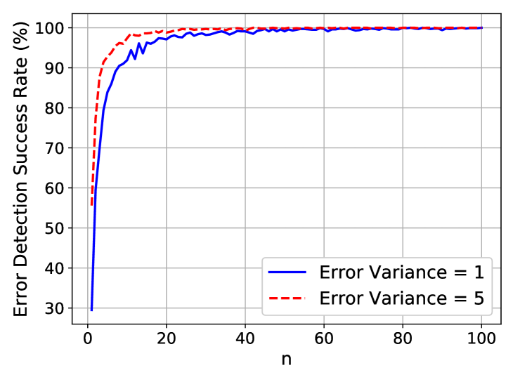
Figure 1: Comparison of the error detection rate with different error variance.

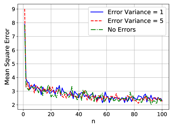
Figure 2: Comparison of the mean square error with different error variance.

IV Numerical Simulations

In this section, we conduct numerical simulations to validate the correctness of the proposed coding scheme. The simulations consider the setting with $\mathsf{N}=16$ nodes, including $\mathsf{T}=5$ colluding nodes, $\mathsf{E}=2$ erased nodes, and $\mathsf{A}=2$ adversarial nodes, satisfying $\mathsf{N}=\mathsf{T}+2\mathsf{A}+\mathsf{E}+1$. We let $\eta=1$, and $\sigma=0.5$. Among the nodes, $\mathsf{E}$ nodes are randomly erased, while $\mathsf{A}=2$ adversarial nodes introduce errors by adding zero-mean Gaussian noise with variance $\mathbb{E}[\sigma^{2}_{e}]$. To analyze the worst-case scenario, we assume that erased nodes and adversarial nodes do not overlap. We select evaluation points $x_{i}=\cos\left(\frac{(2i-1)\pi}{2\mathsf{N}}\right)$. The simulations aim to demonstrate the system performance with increasing $n$, and 1000 simulations are conducted for each $n$ to reduce the effects of randomness. Figure 1 illustrates the error detection success rate versus $n$ with error variance $\mathbb{E}[\sigma^{2}_{e}]\in\{1,5\}$. The success detection rates for both error variances converge to nearly 100 % with increasing $n$, which coincides with the analysis in Section III-D. Besides, the success rate with $\mathbb{E}[\sigma^{2}_{e}]=5$ (the red dotted line) converges more rapidly compared to the success rate with $\mathbb{E}[\sigma^{2}_{e}]=1$ (the blue solid line). This phenomenon, different from that in the finite field, arises because errors of larger magnitude are more readily detected, whereas small errors have a less significant impact on the computation result, even if they remain undetected. Figure 2 compares the mean square error with no adversaries (the green dash-dot line), $\mathbb{E}[\sigma^{2}_{0}]=1$ (the blue solid line) and $\mathbb{E}[\sigma^{2}_{0}]=5$ (the red dotted line). All three lines exhibit similar trends and magnitudes as $n$ increases, showing the effectiveness of the proposed scheme in managing adversarial nodes with varying error magnitudes.

Appendix A

We first consider the ideal case by dropping all $\mathsf{T}$ terms of magnitude $O\left(\frac{1}{n^{2}}\right)$ in the polynomial $p_{A}(x)p_{B}(x)$, and derive a new form of the computation results as follows.

$$\begin{bmatrix}\tilde{C}_{s_{1}}^{\prime}\\ \tilde{C}_{s_{2}}^{\prime}\\ \vdots\\ \tilde{C}_{s_{\mathsf{N}-\mathsf{E}}}^{\prime}\end{bmatrix}=\begin{bmatrix}1&x_{s_{1}}&x_{s_{1}}^{2}&\cdots&x_{1}^{\mathsf{T}}\\ 1&x_{s_{2}}&x_{s_{2}}^{2}&\cdots&x_{s_{2}}^{\mathsf{T}}\\ \vdots&\vdots&\vdots&\ddots&\vdots\\ 1&x_{s_{\mathsf{N}-\mathsf{E}}}&x_{s_{\mathsf{N}-\mathsf{E}}}^{2}&\cdots&x_{s_{\mathsf{N}-\mathsf{E}}}^{\mathsf{T}}\end{bmatrix}\begin{bmatrix}m_{1}\\ m_{2}\\ m_{3}\\ \vdots\\ m_{\mathsf{T}+1}\end{bmatrix},$$ (23)

which constitutes a $(\mathsf{N}-\mathsf{E},\mathsf{T}+1)$ RS code, and $m_{1}=\left(A+R_{1}\right)\left(B+S_{1}\right),m_{2}=\frac{1}{n}\left(S_{2}(A+R_{1})+R_{2}(B+S_{1})\right),\cdots,m_{\mathsf{T}}=\frac{1}{n}(S_{\mathsf{T}}(A+R_{1})+R_{\mathsf{T}}(B+S_{1})),$ $m_{\mathsf{T}+1}=\frac{1}{n^{3/2}}(S_{1}(A+R_{1})+R_{1}(B+S_{1}))$. For this $(\mathsf{N}-\mathsf{E},\mathsf{T}+1)$ RS code, we denote the corresponding message polynomial as $p(\cdot)$ of degree $\mathsf{T}$. We denote $E(\cdot)$ as a monic error locator polynomial of degree $\mathsf{A}$, with coefficients $\{e_{i}\}_{i=0}^{\mathsf{A}-1}$, and ${Q}(\cdot)$, a polynomial of degree $\mathsf{T}+\mathsf{A}$, as the product of the error locator polynomial ${E}(\cdot)$ and message polynomial $p(\cdot)$ with $\{q_{i}\}_{i=0}^{\mathsf{T}+\mathsf{A}}$. Let $Y^{\prime}_{i}\in\mathbb{R}$ denote the messages received by the decoder, where $Y^{\prime}_{i}=\tilde{C}_{i}^{\prime}$ if node $i$ is not an adversary, $Y^{\prime}_{i}\neq\tilde{C}_{i}^{\prime}$ if node $i$ is an adversary. Note that the relation $Y_{s_{i}}^{\prime}E(x_{s_{i}})=Q(x_{s_{i}})$ always holds for any $i\in[\mathsf{N-}\mathsf{E}]$ [8]. As there are $\mathsf{N}-\mathsf{S}=\mathsf{T}+2\mathsf{A}+1$ surviving computation results, we could formulate and solve the following linear system.

$$\mathbf{D}\mathbf{b}=\mathbf{c},$$ (24)

${\mathbf{D}}=\begin{bmatrix}Y^{\prime}_{s_{1}}&x_{s_{1}}Y^{\prime}_{s_{1}}&\cdots&x_{s_{1}}^{\mathsf{A-1}}Y^{\prime}_{s_{1}}&-1&-x_{s_{1}}&\cdots&-x_{s_{1}}^{\mathsf{T}+\mathsf{A}}\\ Y^{\prime}_{s_{2}}&x_{s_{2}}Y^{\prime}_{s_{2}}&\cdots&x_{s_{2}}^{\mathsf{A-1}}Y^{\prime}_{s_{2}}&-1&-x_{s_{2}}&\cdots&-x_{s_{2}}^{\mathsf{T}+\mathsf{A}}\\ \vdots&\vdots&\ddots&\vdots&\vdots&\vdots&\ddots&\vdots\\ Y^{\prime}_{s_{\mathsf{N}-\mathsf{E}}}&x_{s_{\mathsf{N}-\mathsf{E}}}Y^{\prime}_{s_{\mathsf{N}-\mathsf{E}}}&\cdots&x_{s_{\mathsf{N}-\mathsf{E}}}^{\mathsf{A-1}}Y^{\prime}_{s_{\mathsf{N}-\mathsf{E}}}&-1&-x_{s_{\mathsf{N}-\mathsf{E}}}&\cdots&-x_{s_{\mathsf{N}-\mathsf{E}}}^{\mathsf{T}+\mathsf{A}}\\ \end{bmatrix}_{(\mathsf{N}-\mathsf{E})\times(\mathsf{N}-\mathsf{E})}$, $\mathbf{{b}}=\begin{bmatrix}{e}_{0}\\ \vdots\\ {e}_{\mathsf{A}-1}\\ {q}_{0}\\ \vdots\\ {q}_{\mathsf{T}+\mathsf{A}}\end{bmatrix}$, $\mathbf{{c}}=\begin{bmatrix}-x_{s_{1}}^{\mathsf{A}}Y^{\prime}_{s_{1}}\\ -x_{s_{2}}^{\mathsf{A}}Y^{\prime}_{s_{2}}\\ \vdots\\ -x_{s_{\mathsf{N}-\mathsf{A}}}^{\mathsf{A}}Y^{\prime}_{s_{\mathsf{N}-\mathsf{A}}}\end{bmatrix}$. By solving the above equations, we can determine the coefficients of $E(\cdot)$ and $Q(\cdot)$ and then which allows us to identify the error nodes. Note since the entries of $\mathbf{b}$ orrespond directly to these coefficients and the magnitude of the elements in it is $O(1)$.

Then we would like to bound the gap between the true coefficients $\mathbf{b}$ and the derived coefficients $\mathbf{\tilde{b}}$.

Let $\Delta\mathbf{D}=\begin{bmatrix}O\left(\frac{1}{n^{2}}\right)&\cdots&O\left(\frac{1}{n^{2}}\right)&0&\cdots&0\\ O\left(\frac{1}{n^{2}}\right)&\cdots&O\left(\frac{1}{n^{2}}\right)&0&\cdots&0\\ \vdots&\ddots&\vdots&\vdots&\ddots&\vdots\\ O\left(\frac{1}{n^{2}}\right)&\cdots&O\left(\frac{1}{n^{2}}\right)&0&\cdots&0\end{bmatrix}$, $\Delta\mathbf{c}=\begin{bmatrix}O\left(\frac{1}{n^{2}}\right)\\ O\left(\frac{1}{n^{2}}\right)\\ \vdots\\ O\left(\frac{1}{n^{2}}\right)\end{bmatrix}$, and (22) can be rewritten as,

$$(\mathbf{D}+\Delta\mathbf{D})\mathbf{\tilde{b}} =\mathbf{c}+\Delta\mathbf{c}$$

$$\mathbf{D}(\mathbf{\tilde{{b}}}-\mathbf{b})+\Delta\mathbf{D}\mathbf{\tilde{{b}}} =\Delta\mathbf{c}$$

$$\mathbf{D}(\mathbf{\tilde{{b}}}-\mathbf{b}) =\Delta\mathbf{c}-\Delta\mathbf{D}\mathbf{\tilde{{b}}}.$$ (25)

By the property of norm, we have

$$\|\mathbf{\tilde{b}}-\mathbf{b}\|_{\infty}\leq\|\mathbf{D}^{-1}\|_{\infty}\|\Delta\mathbf{c}-\Delta\mathbf{D}\mathbf{\tilde{{b}}}\|_{\infty}.$$ (26)

For $\Delta\mathbf{c}-\Delta\mathbf{D}\mathbf{\tilde{{b}}}$, we have $\|\Delta\mathbf{c}-\Delta\mathbf{D}\mathbf{\tilde{{b}}}\|_{\infty}=O\left(\frac{1}{n^{2}}\right)$ based on the magnitude of $\Delta\mathbf{D}$ and $\Delta\mathbf{c}$. As elements in $\mathbf{D}$ and $\mathbf{D}^{-1}$ would not tend to infinity with increasing $n$, $\|\mathbf{D}^{-1}\|_{\infty}\|\Delta\mathbf{c}-\Delta\mathbf{D}\mathbf{\tilde{{b}}}\|_{\infty}=O\left(\frac{1}{n^{2}}\right)$. Then the distortion between $\{e_{i}\}$ and $\{\tilde{e}_{i}\}$ is upper bounded by an arbitrarily small value, and the correctness of the decoding can be guaranteed as the derived locations will be close to the actual locations.

Then we would like to explore the necessary conditions for an error to remain undetected. For the linear system that omits terms of magnitude $O\left(\frac{1}{n^{2}}\right)$ in (24), any error can be successfully detected. However, in contrast to the coefficients $\mathbf{D}$ and $\mathbf{c}$ in (24), the coefficients in the actual linear system in (22) are $\tilde{\mathbf{D}}=\mathbf{D}+\Delta\mathbf{D}$ and $\tilde{\mathbf{c}}=\mathbf{c}+\Delta\mathbf{c}$, incorporating perturbations $\Delta\mathbf{D}$ and $\Delta\mathbf{c}$. If the magnitude of an error is sufficiently small, specifically the noise variance $\mathbb{E}[\sigma_{e}^{2}(n)]=o\left(\frac{1}{n^{2}}\right)$, such that it is indistinguishable from the perturbations, then the error cannot be detected. Together with the accuracy analysis in Section III-C, such error with magnitude $o\left(\frac{1}{n^{2}}\right)$ does not impact the asymptotically achievable results.

References

- [1] O. Goldreich, “Secure multi-party computation,” Manuscript. Preliminary version, vol. 78, no. 110, pp. 1–108, 1998.
- [2] A. Shamir, “How to share a secret,” Communications of the ACM, vol. 22, no. 11, pp. 612–613, 1979.
- [3] I. S. Reed and G. Solomon, “Polynomial codes over certain finite fields,” Journal of the society for industrial and applied mathematics, vol. 8, no. 2, pp. 300–304, 1960.
- [4] A. Wigderson, M. Or, and S. Goldwasser, “Completeness theorems for noncryptographic fault-tolerant distributed computations,” in Proceedings of the 20th Annual Symposium on the Theory of Computing (STOC’88), 1988, pp. 1–10.
- [5] H. B. McMahan, G. Andrew, U. Erlingsson, S. Chien, I. Mironov, N. Papernot, and P. Kairouz, “A general approach to adding differential privacy to iterative training procedures,” arXiv preprint arXiv:1812.06210, 2018.
- [6] C. Dwork, “Differential privacy,” in International colloquium on automata, languages, and programming. Springer, 2006, pp. 1–12.
- [7] V. R. Cadambe, H. Jeong, and F. P. Calmon, “Differentially private secure multiplication: Hiding information in the rubble of noise,” in 2023 IEEE International Symposium on Information Theory (ISIT). IEEE, 2023, pp. 2207–2212.
- [8] L. R. Welch and E. R. Berlekamp, “Error correction for algebraic block codes,” Dec. 30 1986, uS Patent 4,633,470.
- [9] K. Lee, M. Lam, R. Pedarsani, D. Papailiopoulos, and K. Ramchandran, “Speeding up distributed machine learning using codes,” IEEE Transactions on Information Theory, vol. 64, no. 3, pp. 1514–1529, 2017.
- [10] Q. Yu, M. Maddah-Ali, and S. Avestimehr, “Polynomial codes: an optimal design for high-dimensional coded matrix multiplication,” Advances in Neural Information Processing Systems, vol. 30, 2017.
- [11] R. Tandon, Q. Lei, A. G. Dimakis, and N. Karampatziakis, “Gradient coding: Avoiding stragglers in distributed learning,” in International Conference on Machine Learning. PMLR, 2017, pp. 3368–3376.
- [12] K. Wan, H. Sun, M. Ji, and G. Caire, “Distributed linearly separable computation,” IEEE Transactions on Information Theory, vol. 68, no. 2, pp. 1259–1278, 2021.
- [13] A. Khalesi and P. Elia, “Multi-user linearly separable computation: A coding theoretic approach,” in 2022 IEEE Information Theory Workshop (ITW). IEEE, 2022, pp. 428–433.
- [14] Q. Yu, S. Li, N. Raviv, S. M. M. Kalan, M. Soltanolkotabi, and S. A. Avestimehr, “Lagrange coded computing: Optimal design for resiliency, security, and privacy,” in The 22nd International Conference on Artificial Intelligence and Statistics. PMLR, 2019, pp. 1215–1225.
- [15] R. G. D’Oliveira, S. El Rouayheb, and D. Karpuk, “Gasp codes for secure distributed matrix multiplication,” IEEE Transactions on Information Theory, vol. 66, no. 7, pp. 4038–4050, 2020.
- [16] T. Jahani-Nezhad, M. A. Maddah-Ali, S. Li, and G. Caire, “Swiftagg+: Achieving asymptotically optimal communication loads in secure aggregation for federated learning,” IEEE Journal on Selected Areas in Communications, vol. 41, no. 4, pp. 977–989, 2023.
- [17] H. Akbari-Nodehi and M. A. Maddah-Ali, “Secure coded multi-party computation for massive matrix operations,” IEEE Transactions on Information Theory, vol. 67, no. 4, pp. 2379–2398, 2021.
- [18] W.-T. Chang and R. Tandon, “On the capacity of secure distributed matrix multiplication,” in 2018 IEEE Global Communications Conference (GLOBECOM). IEEE, 2018, pp. 1–6.
- [19] Z. Jia and S. A. Jafar, “On the capacity of secure distributed batch matrix multiplication,” IEEE Transactions on Information Theory, vol. 67, no. 11, pp. 7420–7437, 2021.
- [20] K. Liang, S. Li, M. Ding, F. Tian, and Y. Wu, “Privacy-preserving coded schemes for multi-server federated learning with straggling links,” IEEE Transactions on Information Forensics and Security, 2024.
- [21] M. Soleymani, M. V. Jamali, and H. Mahdavifar, “Coded computing via binary linear codes: Designs and performance limits,” IEEE Journal on Selected Areas in Information Theory, vol. 2, no. 3, pp. 879–892, 2021.
- [22] M. Soleymani, H. Mahdavifar, and A. S. Avestimehr, “Analog lagrange coded computing,” IEEE Journal on Selected Areas in Information Theory, vol. 2, no. 1, pp. 283–295, 2021.
- [23] ——, “Analog secret sharing with applications to private distributed learning,” IEEE Transactions on Information Forensics and Security, vol. 17, pp. 1893–1904, 2022.
- [24] H.-P. Liu, M. Soleymani, and H. Mahdavifar, “Analog multi-party computing: Locally differential private protocols for collaborative computations,” arXiv preprint arXiv:2308.12544, 2023.
- [25] ——, “Differentially private coded computing,” in 2023 IEEE International Symposium on Information Theory (ISIT). IEEE, 2023, pp. 2189–2194.
- [26] R. M. Roth, “Analog error-correcting codes,” IEEE Transactions on Information Theory, vol. 66, no. 7, pp. 4075–4088, 2020.
- [27] A. Jiang, “Analog error-correcting codes: Designs and analysis,” IEEE Transactions on Information Theory, 2024.
- [28] M. Soleymani, R. E. Ali, H. Mahdavifar, and A. S. Avestimehr, “Approxifer: A model-agnostic approach to resilient and robust prediction serving systems,” in Proceedings of the AAAI Conference on Artificial Intelligence, vol. 36, no. 8, 2022, pp. 8342–8350.
- [29] Q. Geng and P. Viswanath, “The optimal noise-adding mechanism in differential privacy,” IEEE Transactions on Information Theory, vol. 62, no. 2, pp. 925–951, 2015.
- [30] C. Dwork, F. McSherry, K. Nissim, and A. Smith, “Calibrating noise to sensitivity in private data analysis,” in Theory of Cryptography: Third Theory of Cryptography Conference, TCC 2006, New York, NY, USA, March 4-7, 2006. Proceedings 3. Springer, 2006, pp. 265–284.
- [31] H. V. Poor, An introduction to signal detection and estimation. Springer Science & Business Media, 2013.
- [32] W. C. Huffman and V. Pless, Fundamentals of error-correcting codes. Cambridge university press, 2010.