Learning Large-Scale Competitive Team Behaviors with Mean-Field Interactions

Abstract.

State-of-the-art multi-agent reinforcement learning (MARL) algorithms such as MADDPG and MAAC fail to scale in situations where the number of agents becomes large. Mean-field theory has shown encouraging results in modeling macroscopic agent behavior for teams with a large number of agents through a continuum approximation of the agent population and its interaction with the environment. In this work, we extend proximal policy optimization (PPO) to the mean-field domain by introducing the Mean-Field Multi-Agent Proximal Policy Optimization (MF-MAPPO), a novel algorithm that utilizes the effectiveness of the finite-population mean-field approximation in the context of zero-sum competitive multi-agent games between two teams. The proposed algorithm can be easily scaled to hundreds and thousands of agents in each team as shown through numerical experiments. In particular, the algorithm is applied to realistic applications such as large-scale offense-defense battlefield scenarios.

1. Introduction

Existing state-of-the-art multi-agent reinforcement learning (MARL) algorithms, such as MADDPG and MAAC Lowe et al. (2017), encounter significant scalability challenges as the number of agents increases. The associated complexities arise due to well-known curse of dimensionality. One promising direction that addresses the scalability challenge in MARL is through mean-field theory, which approximates large-scale agent interactions with the environment at an infinite population limit Huang et al. (2006). Two major areas of mean-field research are the mean-field games (MFGs) Huang et al. (2006); Shao et al. (2024); Guan et al. (2022) which focus on non-cooperative agents, and mean-field control problems (MFC) Huang et al. (2006); Saldi et al. (2023); Sen and Caines (2019), which study fully cooperative scenarios. However, work in mixed collaborative-competitive settings is relatively sparse.

The recent work in Guan et al. (2024) formulated and studied zero-sum mean-field team games (ZS-MFTG), which models large-population teams competing against each other while agents within a team cooperate. In a two-team scenario, Guan et al. (2024) utilized a common-information decomposition Nayyar et al. (2013) to reduce the original problem to training two fictitious team coordinators, making the approach agnostic to the actual number of agents in the team, thus significantly reducing the computational load. The existence of approximate optimal team policies that are identical across agents was also established. However, numerically computing the corresponding team policies is not straightforward. Our work makes a contribution in this direction by leveraging deep reinforcement learning and exploiting theoretical properties of the MFTG obtained in Guan et al. (2024), specifically the identical team policies and the common-information decomposition.

We propose the Mean-Field Multi-Agent Proximal Policy Optimization algorithm (MF-MAPPO), a novel multi-agent RL algorithm that extends PPO to accommodate intra-team cooperation and inter-team competition in large-population scenarios. The proposed algorithm employs a shared actor and critic for each team, with the information commonly available to all agents as inputs.

As shown in extensive numerical experiments, backed by theoretical guarantees from Guan et al. (2024), our method scales efficiently to teams with hundreds or thousands of agents. Notably, the algorithm operates independently of individual agents’ private information and is agnostic to the specific index/identity of each agent. To the best of our knowledge, this is the first algorithm that applies PPO to learning mixed competitive and collaborative mean-field problems.

The main contributions of our work are: 1) the MF-MAPPO algorithm that relies on shared critic and actor to efficiently learn large-scale team games; 2) novel MFTG scenarios (constrained Rock-Paper-Scissor and Battlefield) as future benchmarking for validation of the scalability of different MARL algorithms; 3) demonstration of MF-MAPPO’s superior efficiency and performance over existing MARL algorithms through comprehensive numerical experiments.

2. Related Work

Recent advances in learning mean-field games have resulted in several model-free reinforcement learning algorithms that span from Q-function based policy gradients to value-function based policy optimization techniques. Reference Yang et al. (2020) proposes MF-Q and MF-AC that parameterize the mean-field Q-function by a neural network. However, the mean-field approach proposed in Yang et al. (2020) differs substantially from our formulation, as it defines the mean-field over neighboring actions rather than over the entire state-space.

Along the lines of Q-function based MARL, reference Shao et al. (2024) proposed an extension of the original Deep Deterministic Policy Gradient (DDPG) algorithm Lillicrap et al. (2019), called DDPG-MFTG, to prescribe a team-level policy based on mean-field observations of all teams. We adopt DDPG-MFTG as a baseline and demonstrate that our proposed method consistently outperforms it, both in terms of stability and performance. Notably, DDPG-MFTG has been primarily evaluated in simple grid-world environments with team-decoupled transition dynamics. It has not been evaluated in environments with tightly coupled mean-field interactions or strict collaborative-competitive scenarios like zero-sum games, where a balance between competition and coordination is paramount. Our work, in contrast, demonstrates robustness and superior performance under precisely these settings.

Reference Yardim and He (2024) shows that policy mirror descent (PMD) along with Temporal Difference (TD) learning converges to an approximate Nash Equilibrium of an $N$-player finite horizon dynamic game (FH-DG). This is another instance of Q-function based learning. Although their approach is more general in terms of the reward structure and heterogeneity among agents, the analysis is limited to mean-field games and excludes mixed collaborative-competitive team games. Alternatively, Wang et al. (2022) introduced ECA-Net, a GAN-based method to solve a differential game between two adversarial teams of cooperative players in an attack-defense situation. However, their work focuses on a continuous state-action space setting while we consider an MDP-type problem formulation with strictly conflicting zero-sum rewards.

Closest to the proposed algorithm is the paper Cui et al. (2024), where the authors introduced a PPO-based algorithm for constructing optimal policies in the context of mean-field control. However, Cui et al. (2024) requires the a-priori knowledge of a mapping from the high-level policy to the agent policies which adds an additional computational step to the algorithm; this is in contrast to our method that directly trains MFTGs using a single identical team policy.

Unlike the methods discussed above, our algorithm is centered around a value function based approach and builds upon the successes of PPO and MA-PPO algorithms Schulman et al. (2017); Yu et al. (2022), and extends those to the competitive mean-field team setting. Following the standard PPO architecture, we do not provide the agents’ actions to the critic network, which greatly reduces the size of the neural network. In fact, as we will show later on, it is sufficient to consider a critic network with just the team distributions (mean-fields) as the sole inputs to the network. This also makes the value function network independent of the number of agents, thereby leading to better scalability. As MF-MAPPO employs a shared actor and critic for each team, a single buffer per team suffices for storing team data, thus reducing memory usage and streamlining experience collection without sacrificing the performance of the learned policy. Another key feature of our proposed algorithm is the simultaneous training of both competing teams. Unlike iterative best-response methods Lanctot et al. (2017); Smith et al. (2021), which involve alternate policy updates, simultaneous training allows both teams to adapt to each other’s most recent policies more dynamically.

3. Problem Formulation

3.1. Zero-Sum Mean-Field Team Game

The zero-sum mean-field team game models a discrete-time stochastic game between two large teams of agents Guan et al. (2022). The Blue and Red teams consist of $N_{1}$ and $N_{2}$ identical agents for each team, with the total number of agents $N\hskip-1.4457pt=\hskip-1.4457ptN_{1}\hskip-1.4457pt+\hskip-1.4457ptN_{2}$. Let $X^{N_{1}}_{i,t}\in\mathcal{X}$ and $U^{N_{1}}_{i,t}\in\mathcal{U}$ represent the state and action of Blue agent $i\in[N_{1}]$ at time $t$. Here, $\mathcal{X}$ and $\mathcal{U}$ are the finite state and action spaces of the Blue team. Similarly, $Y^{N_{2}}_{j,t}\in\mathcal{Y}$ and $V^{N_{2}}_{j,t}\in\mathcal{V}$ denote the state and action of Red agent $j\in[N_{2}]$. The joint state-action variables for the Blue and Red teams are denoted as $(\mathbf{X}^{N_{1}}_{t},\mathbf{U}^{N_{1}}_{t})$ and $(\mathbf{Y}^{N_{2}}_{t},\mathbf{V}^{N_{2}}_{t})$, respectively. Here, we use uppercase letters to denote random variables (e.g., $X$, $\mathcal{M}$) and lowercase letters to denote their realizations (e.g., $x$, $\mu$). For a set $E$, we denote the space of probability measures over $E$ as $\mathcal{P}({E})$.

Definition .

The empirical distributions (ED) for the Blue and Red teams are defined as

$$\mathcal{M}^{N_{1}}_{t}(x) =\frac{1}{N_{1}}\sum_{i=1}^{N_{1}}\mathds{1}_{x}(X^{N_{1}}_{i,t}),\quad x\in\mathcal{X},$$ (1a)

$$\mathcal{N}^{N_{2}}_{t}(y) =\frac{1}{N_{2}}\sum_{j=1}^{N_{2}}\mathds{1}_{y}(Y^{N_{2}}_{j,t}),\quad y\in\mathcal{Y},$$ (1b)

where $\mathds{1}_{a}\big{(}{b}\big{)}=1$ if $a=b$ and $0$ otherwise. Specifically, $\mathcal{M}^{N_{1}}_{t}(x)$ gives the fraction of Blue agents at state $x$ and similarly for $\mathcal{N}^{N_{2}}_{t}(y)$. We use $\mathcal{M}_{t}^{N_{1}}=\mathrm{Emp}_{\mu}(\mathbf{X}^{N_{1}}_{t})$ and $\mathcal{N}_{t}^{N_{2}}=\mathrm{Emp}_{\nu}(\mathbf{Y}^{N_{2}}_{t})$ to denote the EDs computed from the given joint states. Note that the $\mathrm{Emp}$ operators remove agent index information, so one cannot determine the state of a specific Blue agent $i$ from $\mathcal{M}^{N_{1}}_{t}$.

We consider weakly-coupled dynamics where the dynamics of each individual agent is coupled with other agents through the EDs Guan et al. (2024). For Blue agent $i$, its stochastic transition is governed by the transition kernel $f_{t}:\mathcal{X}\times\mathcal{U}\times\mathcal{P}(\mathcal{X})\times\mathcal{P}(\mathcal{Y})\rightarrow\mathcal{P}(\mathcal{X})$ so that

$$\mathbb{P}(X_{i,t+1}^{N_{1}}=x_{i,t+1}^{N_{1}} |U_{i,t}^{N_{1}}=u_{i,t}^{N_{1}},\mathbf{X}_{t}^{N_{1}}=\mathbf{x}_{t}^{N_{1}},\mathbf{Y}_{t}^{N_{2}}=\mathbf{y}_{t}^{N_{2}})$$

$$=f_{t}(x_{i,t+1}^{N_{1}}|x_{i,t}^{N_{1}},u_{i,t}^{N_{1}},\mu^{N_{1}}_{t},\nu^{N_{2}}_{t}),$$ (2)

where $\mu^{N_{1}}_{t}=\mathrm{Emp}_{\mu}(\mathbf{x}_{t}^{N_{1}})$ and $\nu^{N_{2}}_{t}=\mathrm{Emp}_{\nu}(\mathbf{y}_{t}^{N_{2}})$. Similarly, the dynamics of Red agent $j$ is governed by the transition kernel $g_{t}:\mathcal{Y}\times\mathcal{V}\times\mathcal{P}(\mathcal{X})\times\mathcal{P}(\mathcal{Y})\rightarrow\mathcal{P}(\mathcal{Y})$. All agents in the Blue team receive an identical weakly-coupled team reward, i.e., $r_{t}\triangleq r_{t}(\mu_{t},\nu_{t}):\mathcal{P}(\mathcal{X})\times\mathcal{P}(\mathcal{Y})\to\mathbb{R}$. Following the zero-sum structure, the Red team agents receive $-r_{t}(\mu_{t},\nu_{t})$ as their rewards. We assume that the Blue (Red) team is the maximizing (minimizing) team.

Figure 1 depicts a battlefield scenario of an MFTG between two teams (Blue and Red) on an $n\times n$ grid world.

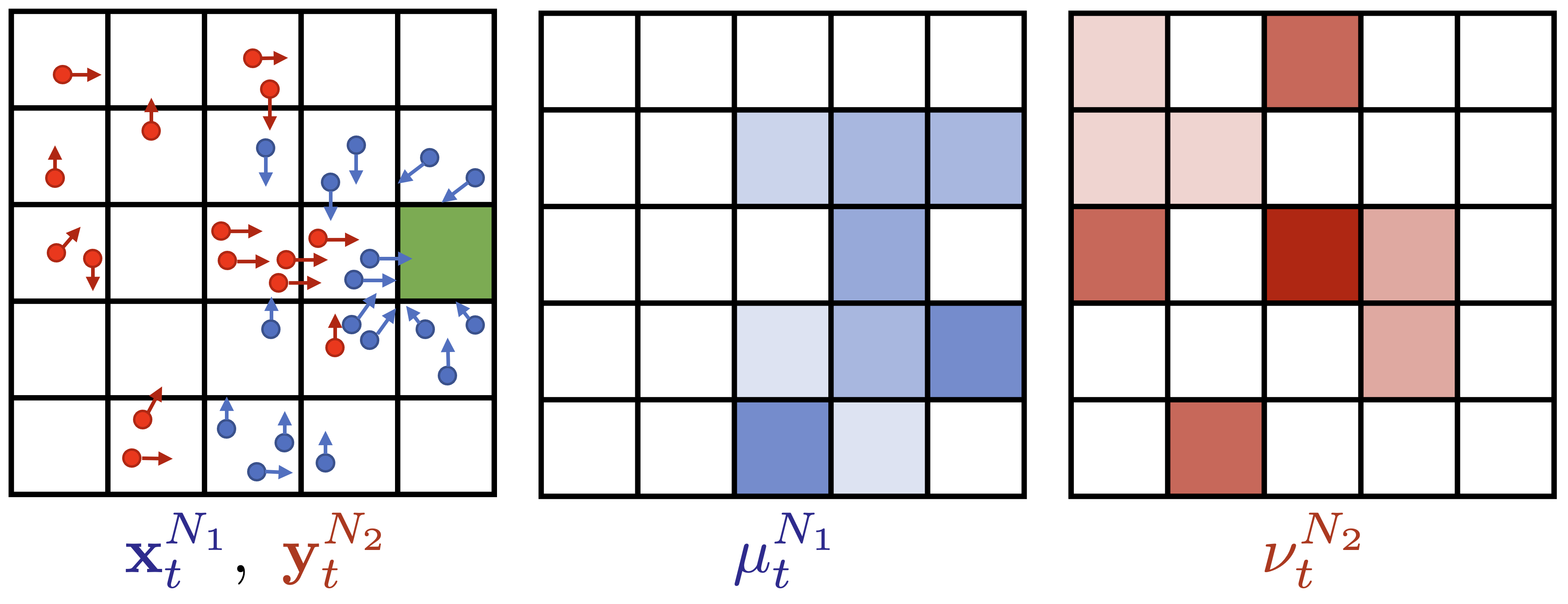
Figure 1. Battlefield Scenario as an example of ZS-MFTG.

Battlefield Scenario as an example of ZS-MFTG.

3.2. Large-Population Optimization

We consider a mean-field sharing information structure Arabneydi and Mahajan (2015), where each agent observes its own state and the two team EDs, where the EDs serve as common information accessible to both teams. Specifically, the Blue and Red agents seek to construct mixed Markov policies with the following structure

$$\phi_{i,t} :\mathcal{U}\times\mathcal{X}\times\mathcal{P}(\mathcal{X})\times\mathcal{P}(\mathcal{Y})\to[0,1],$$ (3a)

$$\psi_{j,t} :\mathcal{V}\times\mathcal{Y}\times\mathcal{P}(\mathcal{X})\times\mathcal{P}(\mathcal{Y})\to[0,1],$$ (3b)

where the Blue policy $\phi_{i,t}(u|x_{i,t}^{N_{1}},\mu^{N_{1}}_{t},\nu^{N_{2}}_{t})$ dictates the probability that Blue agent $i$ selects action $u$ given its state $x_{i,t}^{N_{1}}$ and the observed team EDs $\mu^{N_{1}}_{t}$ and $\nu^{N_{2}}_{t}$. Note that each agent’s individual state is its private information, while the team EDs are the common information available to all $N$ agents.

Let $\Phi_{t}$ ($\Psi_{t}$) denote the set of individual Blue (Red) policies at time $t$. We define the Blue team policy $\phi^{N_{1}}_{t}\!=\!\{\phi_{i,t}\}_{i=1}^{N_{1}}$ as the collection of the $N_{1}$ Blue agent individual policies, and denote the set of Blue team policies as $\Phi^{N_{1}}_{t}\!=\!\times_{N_{1}}\Phi_{t}$. Similarly, the Red team policy is denoted as $\psi_{t}^{N_{2}}\in\Psi_{t}^{N_{2}}\!=\!\times_{N_{2}}\Psi_{t}$.

Definition (Identical team policy).

The Blue team policy $\phi^{N_{1}}_{t}=(\phi^{N_{1}}_{1,t},\ldots,\phi^{N_{1}}_{N_{1},t})$ is an identical, if $\phi_{i_{1},t}=\phi_{i_{2},t}$ for all time $t$ and $i_{1},i_{2}\in[N_{1}]$. We denote the set of identical Blue team policies as $\Phi$.

The definition and notation extend naturally to the Red team, and the set of identical Red team policies is denoted as $\Psi$.

The performance of the team policy pair $(\phi^{N_{1}},\psi^{N_{2}})$ is given by the expected cumulative reward

$$J^{N,\phi^{N_{1}},\psi^{N_{2}}}\big{(}\mathbf{x}_{0}^{N_{1}},\mathbf{y}_{0}^{N_{2}}\big{)}=\mathbb{E}_{{\phi^{N_{1}},\psi^{N_{2}}}}\Big{[}\sum_{t=0}^{T}r_{t}(\mathcal{M}^{N_{1}}_{t},\mathcal{N}^{N_{2}}_{t})\Big{|}\mathbf{x}_{0}^{N_{1}},\mathbf{y}^{N_{2}}_{0}\!\Big{]}.$$

When the Blue team considers its worst-case performance, we have the following max-min optimization:

$$\hskip-0.72229pt\underline{J}^{N*}(\mathbf{x}_{0}^{N_{1}},\mathbf{y}_{0}^{N_{2}})=\max_{\mathbf{\phi}^{N_{1}}\in\Phi^{N_{1}}}\min_{\mathbf{\psi}^{N_{2}}\in\Psi^{N_{2}}}J^{N,\phi^{N_{1}},\psi^{N_{2}}}\hskip-1.4457pt(\mathbf{x}_{0}^{N_{1}}\hskip-3.61371pt,\mathbf{y}_{0}^{N_{2}}),\hskip-7.22743pt$$ (4)

where $\underline{J}^{N*}$ is the lower game value for the finite-population game. Similarly, the minimizing Red team considers a min-max optimization problem, which leads to the upper game value. Note that we allow both teams to follow non-identical team policies in (4).

3.3. Infinite-Population Solution

To reduce the complexity of team policy optimization domains in (4), the authors of Guan et al. (2024) proposed to examine team behaviors under identical team policies at the infinite-population limit. It was shown that the team joint states can be represented using the team population distribution, which coincides with the state distribution of a typical agent. Such distributions are referred to as the mean-fields (MFs), and we denoted them as $\mu_{t}$ and $\nu_{t}$ for the Blue and Red teams, respectively. As proved in Guan et al. (2024), MFs induced by identical team policies in an infinite-population game closely approximate the EDs induced by non-identical team policies in the corresponding finite-population game, which justifies the simplification of the optimization domain in (4) to identical team policies.

For the infinite-population game, the performance of the identical team policies $(\phi,\psi)\in\Phi\times\Psi$ is measured by

$$J^{\phi,\psi}(\mu_{0},\nu_{0})=\sum_{t=0}^{T}r_{t}(\mu_{t},\nu_{t}),$$ (5)

where $\mu_{t}$ and $\nu_{t}$ follow a deterministic dynamics Guan et al. (2024) similar to the state distribution propagation of a controlled Markov chain. The worst-case performance of the Blue team in this infinite-population game is then given by the lower game value

$$\underline{J}^{*}(\mu_{0},\nu_{0})=\max_{\phi\in\Phi}\;\min_{\psi\in\Psi}\leavevmode\nobreak\ J^{\phi,\psi}(\mu_{0},\nu_{0}),$$ (6)

where the optimization domain is restricted to identical team policies. Reference Guan et al. (2024) exploited the simplified optimization domain in (6) and proposed to transform the optimization to an equivalent zero-sum game between two fictitious coordinators. The optimal identical team policies can then be solved via dynamic programming. The following performance guarantees was established in Guan et al. (2024).

The optimal identical Blue team policy $\phi^{*}$ obtained from the equivalent zero-sum coordinator game is an $\epsilon$-optimal Blue team policy. Formally, for all joint states $\mathbf{x}^{N_{1}}$ and $\mathbf{y}^{N_{2}}$,

$$\min_{\psi^{N_{2}}\in\Psi^{N_{2}}}J^{N,\phi^{*},\psi^{N_{2}}}(\mathbf{x}^{N_{1}},\mathbf{y}^{N_{2}})\geq\underline{J}^{N*}(\mathbf{x}^{N_{1}},\mathbf{y}^{N_{2}})-\mathcal{O}\Big{(}\frac{1}{\sqrt{\underline{N}}}\Big{)}$$ (7)

where $\underline{N}=\min\{N_{1},N_{2}\}$.

This result ensures that identical team policies resulting from the solution of the equivalent zero-sum coordinator game are still $\epsilon$-optimal for the original max-min optimization problem in (4). From Theorem 3.3 we can further show that the performance of the optimal identical policy learned from the finite population ZS-MFTG remains within an $\epsilon$-bound of the identical policies derived from the optimal coordinator game.

[] The value of the optimal identical Blue team policy $\phi^{*}_{\mathrm{finite}}$ obtained from the finite population game is within $\epsilon$ of the value of the optimal identical Blue team policy $\phi^{*}$ obtained from the equivalent zero-sum coordinator game. Formally, for all joint states $\mathbf{x}^{N_{1}}$ and $\mathbf{y}^{N_{2}}$,

$$\min_{\psi^{N_{2}}}J^{N,\phi^{*}_{\mathrm{finite}},\psi^{N_{2}}}(\mathbf{x}^{N_{1}},\mathbf{y}^{N_{2}})-\min_{\psi^{N_{2}}}J^{N,\phi^{*},\psi^{N_{2}}}(\mathbf{x}^{N_{1}},\mathbf{y}^{N_{2}})\leq\epsilon,$$ (8)

where $\epsilon=\mathcal{O}({1}/{\sqrt{\underline{N}}})$ and $\underline{N}=\min\{N_{1},N_{2}\}$.

The first figure depicts the individual agents’ local positions, with the target marked by the green colored cell. The subsequent figures illustrate the state distributions $\mu^{N_{1}}_{t}$ and $\nu^{N_{2}}_{t}$ of both teams, which constitute the common information available to the agents of both teams. The agents interact based on weakly-coupled dynamics, which depend only on $\mu^{N_{1}}_{t}$ and $\nu^{N_{2}}_{t}$ as described in (3.1). In this typical scenario of an MFTG, each agent takes its action after observing its own local position and the common (i.e., mean-field) information, in order to achieve its own team’s objective.

4. Mean-Field Multi-Agent Proximal Policy Optimization

Motivated by Theorem 3.3, we present an algorithm to learn the optimal identical team policy. We build our algorithm based on the proximal policy optimization (PPO) framework due to its simplicity and effectiveness. While PPO has shown promising performance in cooperative tasks including mean-field control problems Yu et al. (2022); Cui et al. (2024), its application in mixed competitive-collaborative scenarios is less studied, especially in the MFTG settings. In the sequel, we introduce our key contribution: the MFTG learning algorithm, which we refer to as Mean-Field Multi-Agent Proximal Policy Optimization (MF-MAPPO).

We initialize two pairs of actor-critic networks, one for each team, deployed to learn the identical policy used by each team (see Figure 2). Specifically, we introduce a minimally-informed critic network by exploiting the shared mean-field information. The key point to note here is that we only require the common information for the critic network in order to learn the value function (Proposition 4.1). Furthermore, the private information available to each agent only individually enters the actor during training. This results in neural networks that scale well with the number of agents.

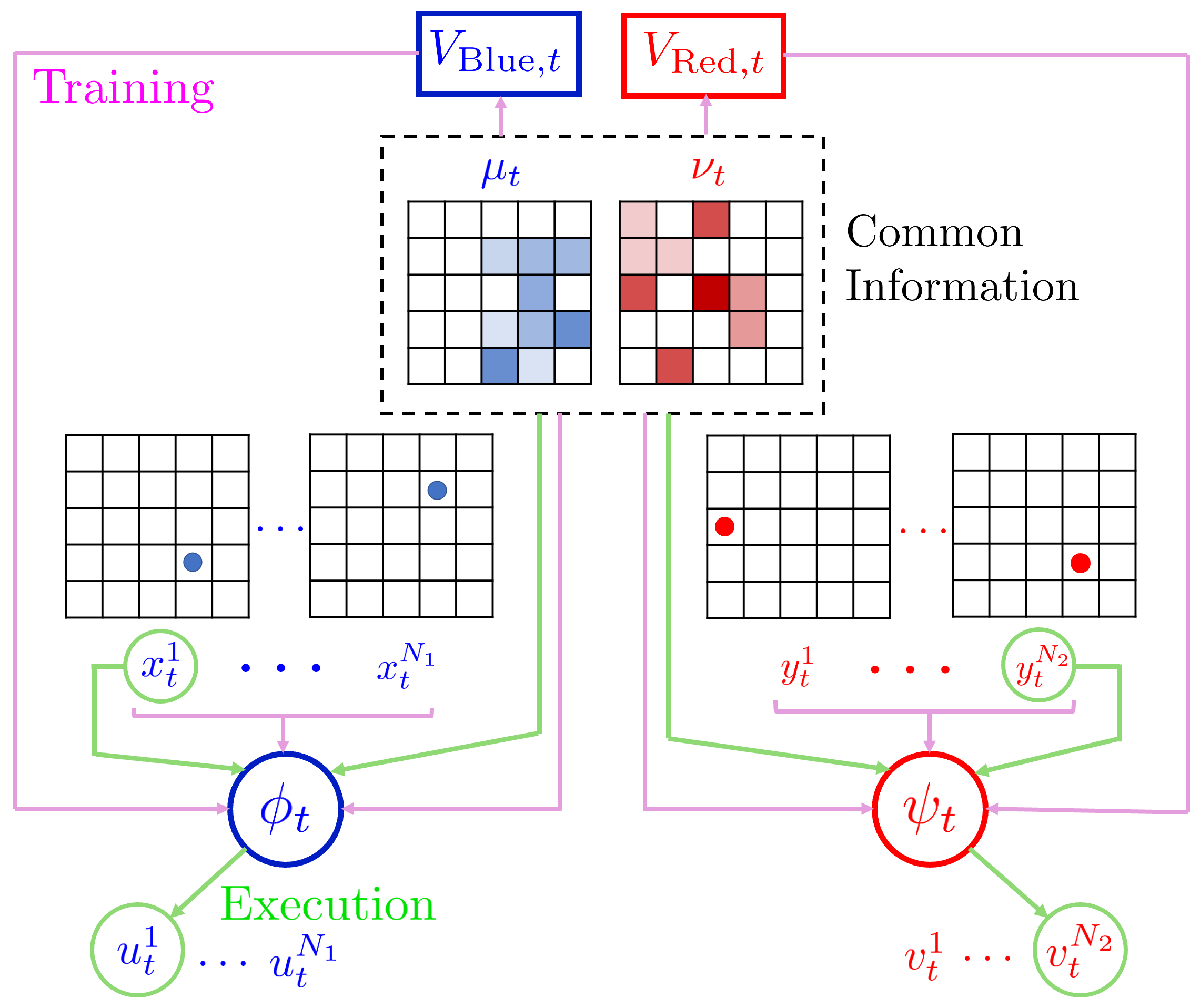
Figure 2. Overview of the architecture of MF-MAPPO.

Schematic for the Actor-Critic Network in MF-MAPPO.

4.1. Minimally-Informed Critic

The MF-MAPPO critic network of the Blue team evaluates the value function $V_{\text{Blue}}(\mu,\nu)$, which depends only on the common information, and is independent of the joint agent states and actions. We use the parameter vector $\zeta_{\text{Blue}}$ to parameterize the critic network while minimizing the MSE loss

$$L_{\text{critic}}(\zeta_{\text{Blue}})=\frac{1}{|B|}\sum_{k=1}^{|B|}\Bigl{(}V_{\text{Blue}}(\mu_{k},\nu_{k}|\zeta_{\text{Blue}})-\hat{R}_{\text{Blue},k}\Bigr{)}^{2},$$ (9)

where the optimization is performed over a mini-batch of size $B$ and $\hat{R}_{\text{Blue},k}$ is the discounted reward-to-go for sample $k$. The reward-to-go for sample $k$ obtained at a time step $t$ is computed using Monte-Carlo roll-outs starting at $t$ until the episode ends, and is given by $\hat{R}_{\text{Blue},k}=\sum_{t^{\prime}=t}^{T}\gamma^{t^{\prime}-t}r_{t}(\mu_{t},\nu_{t})$ Tamar et al. (2016). Similar learning rules apply to the Red team critic $V_{\text{Red}}(\mu,\nu|\zeta_{\text{Red}})$ with the negative reward $\hat{R}_{\text{Red},k}=-\hat{R}_{\text{Blue},k}$ due to the zero-sum structure.

The following proposition follows immediately from the expression of the team reward (5) and the use of identical team policies, and justifies the deployment of a minimally-informed critic network with only the mean-fields as inputs.

Proposition

Let $\mu^{N_{1}}_{t}$, and $\nu^{N_{2}}_{t}$ denote the EDs of a finite-population game obtained from identical Blue and Red team policies $\phi_{t}\in\Phi_{t}$ and $\psi_{t}\in\Psi_{t}$, respectively. The team reward structure admits a critic that depends only on $\mu^{N_{1}}_{t}$ and $\nu^{N_{2}}_{t}$. Specifically, for each Blue team agent $i\in\{1,2,\ldots,N_{1}\}$, the individual critic value function $V_{i,t}^{N_{1},\phi_{t}}(x_{i,t},\mu^{N_{1}}_{t},\nu^{N_{2}}_{t})$ satisfies

$$V_{i,t}^{N_{1},\phi_{t}}(x_{i,t},\mu^{N_{1}}_{t},\nu^{N_{2}}_{t})=V^{N_{1},\phi_{t}}_{{\rm Blue},t}(\mu^{N_{1}}_{t},\nu^{N_{2}}_{t}),$$ (10)

where $V^{N_{1},\phi_{t}}_{{\rm Blue},t}(\mu_{t},\nu_{t})$ is the team-level critic.

The above proposition extends to the Red team critic network. Importantly, it reduces the learning problem to one critic network per team. Specifically, the shared team reward structure along with the assumption of homogeneous agents in each team enables us to evaluate the performance of a team’s agent using the minimally-informed critic—even if the individual agent has additional local observations such as their actions and private states.

4.2. Shared-Team Actor

We consider a single-actor network for each team to learn the identical team policies. According to Guan et al. (2024), identical policies derived from an equivalent coordinator game can approximate team behaviors induced by non-identical ones. A single coordinator policy corresponds to the probability distribution over actions for each state, conditioned on a given mean-field. As a result, its dimensionality scales with the joint state-action space, leading to substantial computational overhead and degraded empirical performance of the policy network. Notably, DDPG-MFTG adopts this formulation, but, as demonstrated later in the numerical examples section, its performance is suboptimal.

Furthermore, while the coordinator game serves as a valuable theoretical construct, we found it more practical and computationally efficient to learn finite-population local identical policies in place of coordinator policies. These policies continue to respect the underlying mean-field information-sharing structure, while significantly reducing complexity and improving tractability in practice. Theorem 3.3 ensures performance guarantees.

The actor network maximizes a PPO-based objective with an entropy term to encourage exploration Schulman et al. (2017); Huang et al. (2022), which decays during training as teams learn reward-maximizing policies. It has also been shown in the mean-field game literature that entropy regularization stabilizes the learning process Cui and Koeppl (2022); Guan et al. (2022). Since the agents are permutation invariant and an identical policy is being learned for each team, a single buffer per team suffices for storing observations and actions, thereby reducing memory overhead and simplifying the experience collection pipeline.

The PPO-based objective function of the Blue actor is given by:

$$L(\theta_{\text{Blue}})=\frac{1}{|B|} \sum_{k=1}^{|B|}\Big{[}\text{min}\Bigl{(}g_{k}(\theta_{\text{Blue}})A_{k},\operatorname{clip}_{[1-\epsilon,1+\epsilon]}(g_{k}(\theta_{\text{Blue}}))A_{k}\Bigr{)}$$

$$\qquad\qquad\qquad\qquad+\omega S(\phi_{\theta_{\text{Blue}}}(x_{k},\mu_{k},\nu_{k}))\Big{]},$$ (11)

where,

$$g(\theta)=\frac{\phi_{\theta}(u|x,\mu,\nu)}{\phi_{\theta^{\text{old}}}(u|x,\mu,\nu)},$$

and $A_{k}$ is the generalized advantage function estimate function Schulman et al. (2018). The tunable parameter $\omega$ weighs the contribution of the entropy term, which is given by

$$S\big{(}\phi_{\theta}(x,\mu,\nu)\big{)}=-\mathbb{E}_{u\sim\mathcal{U}}\Biggl{[}\sum_{u}\phi_{\theta}(u|x,\mu,\nu)\log\phi_{\theta}(u|x,\mu,\nu)\Biggr{]}.$$

We decay $\omega$ as training progresses. A similar learning rule is used for the Red team actor network. Algorithm 1 presents the pseudo-code of the MF-MAPPO algorithm.

Algorithm 1 Mean-Field Multi-Agent Proximal Policy Optimization (MF-MAPPO)

Initialize: NN parameters $\{\theta_{\text{Blue}},\zeta_{\text{Blue}}\}$ and $\{\theta_{\text{Red}},\zeta_{\text{Red}}\}$; step size sequences $\{\alpha_{m}\}$ and $\{\beta_{m}\}$; entropy decay sequence $\{\omega_{m}\}$

for $i=1,2,\ldots$ do

  $(\phi_{\theta_{\text{Blue}}^{\text{old}}},\psi_{\theta_{\text{Red}}^{\text{old}}})\leftarrow(\phi_{\theta_{\text{Blue}}},\psi_{\theta_{\text{Red}}})$

  for $t=0,1,\ldots,T_{\text{rollout}}$ do

   Sample joint actions

   $u_{i,t}\sim\phi_{\theta_{\text{Blue}}^{\text{old}}}(x_{i,t},\mu_{t}^{N_{1}},\nu_{t}^{N_{2}})$, $v_{j,t}\sim\psi_{\theta_{\text{Red}}^{\text{old}}}(y_{j,t},\mu_{t}^{N_{1}},\nu_{t}^{N_{2}})$

   Step environment according to kernels $(f_{t},g_{t})$

   Collect samples $(\mathbf{x}_{t+1}^{N_{1}},\mathbf{y}_{t+1}^{N_{2}},\mu^{N_{1}}_{t+1},\nu^{N_{2}}_{t+1},\mathbf{u}_{t}^{N_{1}},\mathbf{v}_{t}^{N_{2}},r_{t})$

  end for

  for $K$ epochs do

   Update $\{\theta_{\text{Blue}},\zeta_{\text{Blue}}\}$ and $\{\theta_{\text{Red}},\zeta_{\text{Red}}\}$ using (9-4.2)

  end for

end for

Return: $(\phi_{\theta_{\text{Blue}}},\psi_{\theta_{\text{Red}}})$

4.3. Scalability of MF-MAPPO

We further demonstrate the scalability of MF-MAPPO as a direct consequence of Theorem 3.3, by showing that, under certain conditions, the learned team policies generalize to varying population sizes $(\tilde{N}_{1},\tilde{N}_{2})$ while maintaining performance guarantees.

Remark 0.

Let $\mathcal{G}_{1}$ denote the finite-population game where the agents utilize the identical team policies $\phi^{*}_{t}$ and $\psi^{*}_{t}$ derived from the equivalent, infinite-population, zero-sum coordinator game, and let the finite-population game $\mathcal{G}_{2}$ with the same state-action space, dynamics, and rewards, but with population sizes $\tilde{N}_{1}$ and $\tilde{N}_{2}$ such that ${\tilde{N}_{1}}/{\tilde{N}_{2}}={N_{1}}/{N_{2}}$ and $\min(\tilde{N}_{1},\tilde{N}_{2})\geq\min(N_{1},N_{2})$. Then, the policies $\phi^{*}_{t}$ and $\psi^{*}_{t}$ remain ${\epsilon}$-optimal for the game $\mathcal{G}_{2}$.

Remark 4.3 describes policies from the equivalent coordinator game. Empirically, we show that identical team policies from the finite-population ZS-MFTG (Theorem 3.3) yield similar results. This allows MF-MAPPO to be trained on a smaller population and deployed to larger teams without additional tuning, significantly reducing computational costs while maintaining performance consistency and generalizability across different population sizes.

5. Numerical Experiments

In this section, we present several large-population scenarios to demonstrate the efficacy of MF-MAPPO. The first two scenarios are mean-field extensions of the rock-paper-scissors game Raghavan (1994) with different action spaces. For these examples, we can analytically compute the mean-field trajectory induced by the equilibrium/optimal policies, and thus use these scenarios to validate the optimality of MF-MAPPO. We then present a more complex battlefield scenario where the Blue and Red teams play an attack-defense game as shown in Figure 1. This scenario has higher (finite) dimensional state and action spaces and the teams are required to learn more complex collective behaviors.

5.1. Rock-Paper-Scissors (RPS)

We first extend the two-player Rock-Paper-Scissors (RPS) game Raghavan (1994) to a game played between two populations. The state space of each individual agent is $\mathcal{S}=\{\texttt{R,P,S}\}$, representing rock, paper, and scissors, respectively. Let $\mu,\nu\in\mathcal{P(S)}$ denote the EDs for the Blue and Red teams. Following the mean-field sharing information structure, an agent observes its local state and the EDs of both teams. The action space, $\mathcal{A}=\{\texttt{CW},\texttt{CCW},\texttt{Stay}\}$, allows agents to either move clockwise, counter-clockwise, or remain idle, respectively.

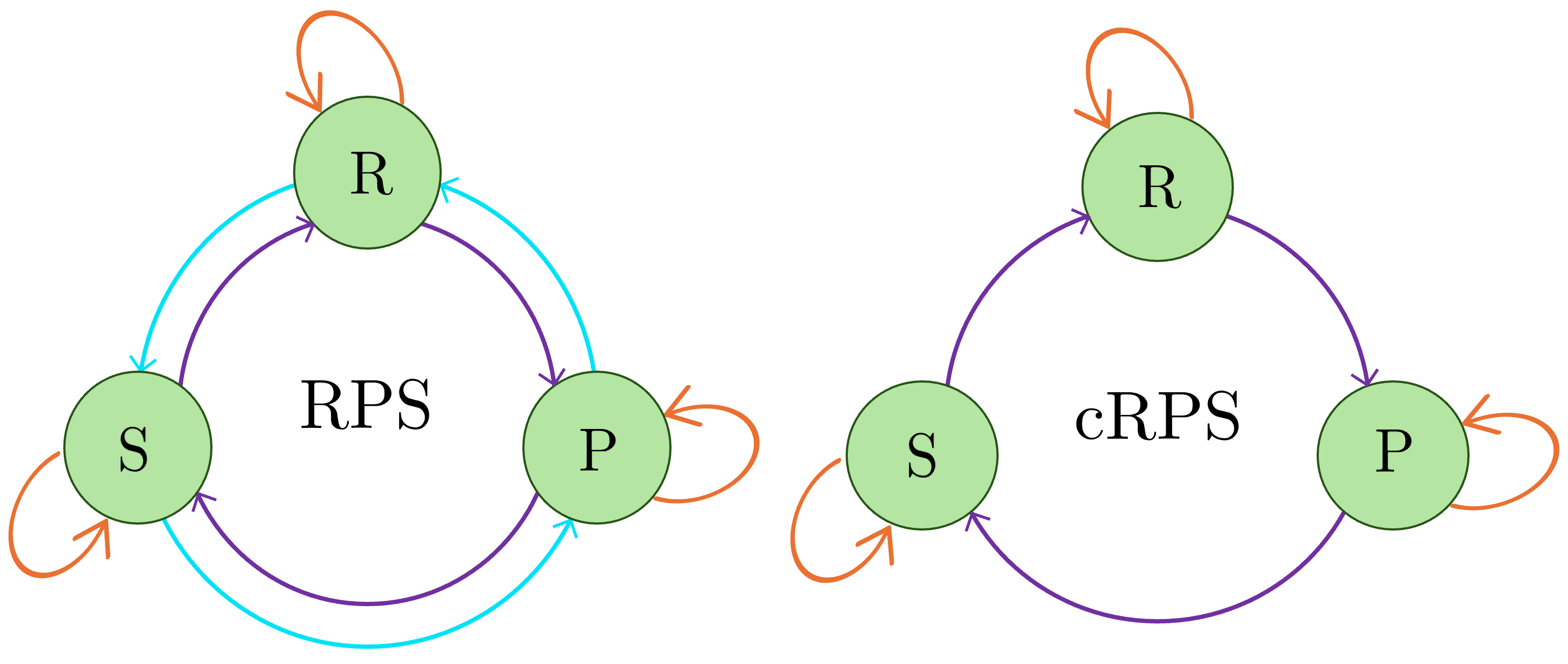
Figure 3. States and actions for RPS and cRPS.

States and Actions for RPS and cRPS

We assume deterministic transitions, where each action leads to a unique next state deterministically. For example, if an agent at R takes action CW, it will deterministically end in state P, as shown in Figure 3. At each time step $t$, the Blue team receives a team reward $r_{t}(\mu_{t},\nu_{t})={\mu}_{t}^{\mbox{\tiny\sf T}}A{\nu}_{t}$ where $A$ is the standard RPS payoff matrix given by $A=[0,-1,1;1,0,-1;-1,1,0]$. We let the Blue team maximize the expected cumulative reward while the Red team minimizes it. The Nash equilibrium for this population-based RPS game is the uniform population distribution $[1/3,1/3,1/3]$ over the 3 states Raghavan (1994); Osborne (2004).

We compare MF-MAPPO with DDPG-MFTG Shao et al. (2024) based on the training time, average test rewards and attainment of the computed Nash distributions for $N_{1}=N_{2}=1,000$ agents. A key distinction between the two algorithms lies in their design philosophy: DDPG-MFTG relies on a mean-field oracle that provides the next mean-field given the current team policy—an object that exists only in the infinite population limit and cannot be directly simulated. In contrast, MF-MAPPO is trained directly within a simulated finite-population environment. DDPG-MFTG introduces “central players” that observe mean-field distributions and output deterministic local policies (akin to the role of the coordinator) via a Q-function, following the standard DDPG architecture. Crucially, in DDPG-MFTG, the input to the Q-function for a given team consists of the mean-field information of all teams, along with only the local policy of the team itself. This contrasts with multi-agent extensions of DDPG (e.g., MADDPG), which also incorporates local policy information of other teams.

Furthermore, the DDPG-MFTG policy is updated at every time step post-exploration without any explicit clipping or regularization mechanisms to constrain policy updates. This lack of stabilization—combined with the high computational complexity and limited inter-team policy awareness—contributes to the algorithm’s training instability and poor generalization, especially in complex environments as we discuss below.

We exclude MADDPG Lowe et al. (2017) from our comparison, as it scales poorly to hundreds or thousands of agents due to its reliance on all agents’ local and global observations and actions as inputs to its critic networks.

From the learning curves in Figure 4 one can see that the DDPG-MFTG algorithm failed to converge to the analytical game value of zero, while MF-MAPPO almost immediately attained the Nash game value. However, as shown in Table 1, MF-MAPPO does take slightly longer to train since, unlike DDPG-MFTG, since MF-MAPPO avoids mini-batch training, following Yu et al. (2022).

We tested the learned policy with a fixed initial distribution $\mu_{t=0}=[1,0,0]^{\mbox{\tiny\sf T}}$ and $\nu_{t=0}=[0,1,0]^{\mbox{\tiny\sf T}}$, and the resulting trajectories are visualized in Figure 5. All simulations were run for 150 instances. The trajectories of the Blue and Red team ED are depicted in cyan and pink, respectively, alongside the mean trajectory. The randomness in these trajectories arises from the finite-population approximation under a stochastic optimal policy, resulting in stochastic EDs. As shown in Figures 4 and 5, DDPG-MFTG diverges from the Nash equilibrium whereas MF-MAPPO converges immediately.

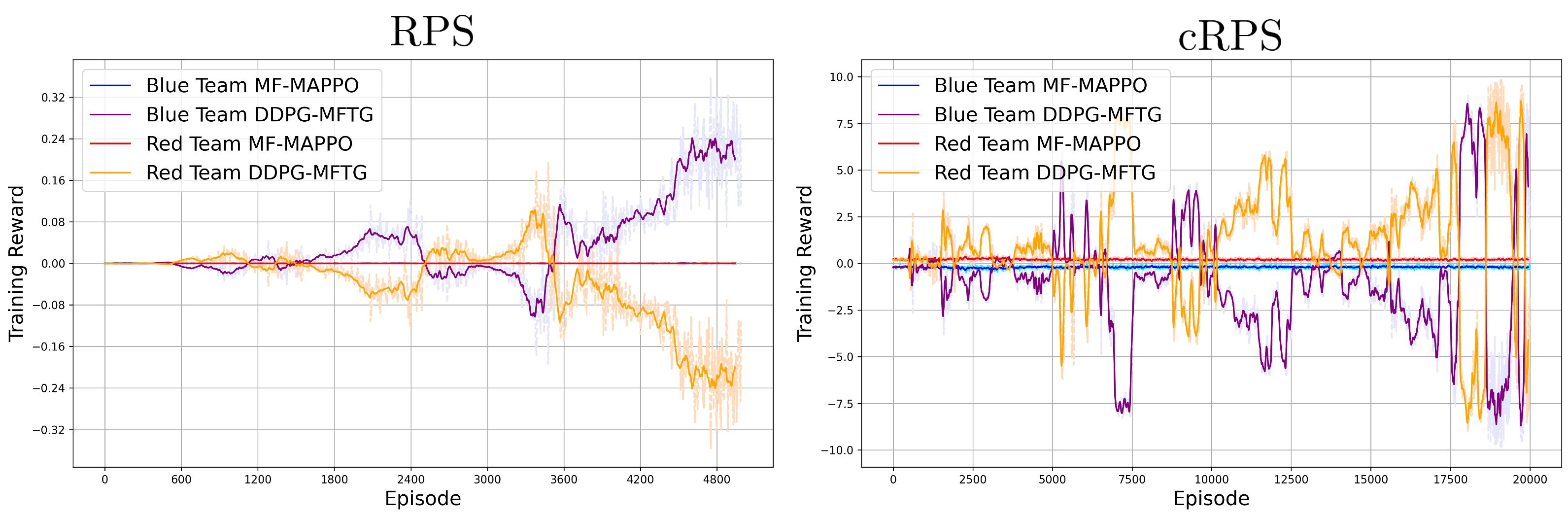
Figure 4. Training reward curves for RPS and cRPS.

Training Reward Curve for RPS where DDPG-MFTG exhibits severe oscillations.

Table 1. Performance Comparison for RPS

Approach	Training Time	Average Reward	NE Attained?
MF-MAPPO	5min 17s	0.0	✓
DDPG-MFTG	1min 34s	0.334	✗

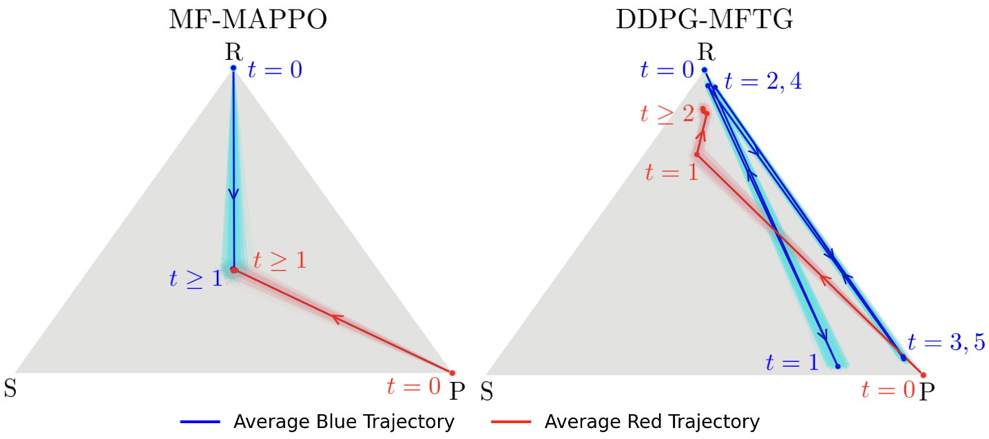
Figure 5. ED trajectories induced by learned team policies on the state distribution simplex. Mean trajectories are averaged based on the 150 runs from fixed initialization $\mu_{t=0}=[1,0,0]^{\mbox{\tiny\sf T}}$ and $\nu_{t=0}=[0,1,0]^{\mbox{\tiny\sf T}}$; $N_{1}=N_{2}=1,000$.

Comparison of trajectories on a 3D simplex for RPS using MF-MAPPO and DDPG-MFTG for 150 initializations.

5.2. Constrained Rock-Paper-Scissors (cRPS)

We now consider a non-trivial modification to the RPS problem by restricting the action space to $\mathcal{A}=\{\texttt{CW},\texttt{Stay}\}$. As shown in Figure 3, with this restricted action space, the teams cannot immediately achieve their desired uniform distribution and need to strategically plan for the intermediate distributions before reaching the desired target uniform distribution. We again consider the fixed initial distributions ${\mu}_{t=0}=[1,0,0]^{\mbox{\tiny\sf T}}$ and ${\nu}_{t=0}=[0,1,0]^{\mbox{\tiny\sf T}}$. One may obtain analytically the conditions for the optimal trajectories of the cRPS game for these initial conditions.

Proposition

With initial conditions ${\mu}_{t=0}=[1,0,0]^{\mbox{\tiny\sf T}}$ and ${\nu}_{t=0}=[0,1,0]^{\mbox{\tiny\sf T}}$, all mean-field optimal trajectories satisfy ${\mu}_{t}^{*}={\nu}_{t}^{*}=[\frac{1}{3},\frac{1}{3},\frac{1}{3}]^{\mbox{\tiny\sf T}}$ for all $t\geq 2$, and ${\mu}^{*}_{1}=[0,1-\eta,\eta]^{\mbox{\tiny\sf T}}$ where $\eta\in[\frac{1}{3},\frac{2}{3}]$ and ${\nu}^{*}_{1}=[0,\frac{2}{3},\frac{1}{3}]^{\mbox{\tiny\sf T}}$. Furthermore, the unique game value is given by $-\frac{1}{3}$.

Figure 6 shows the trajectories over ten time steps induced by the team policies learned by MF-MAPPO and DDPG-MFTG. Using MF-MAPPO, the teams successfully reach the uniform distribution from the initial condition in Proposition 5.2, as shown in Figure 6, while the DDPG-MFTG’s trajectories diverge. For MF-MAPPO, the teams follow the optimal trajectory at $t=1$, and the target optimal distribution is reached within three to four time steps. The transient time can be attributed to the finite population approximation and the entropy term in the optimization problem. Despite this, the Blue team’s game value after training (-0.331) closely matches the theoretical value $-{1}/{3}$. Figure 7 shows trajectories for various population sizes using identical policies trained on $N_{1}=N_{2}=1,000$ with MF-MAPPO. As the population size increases, the trajectories exhibit reduced noise and variance while maintaining strong performance, consistent with the scalability result in Remark 4.3.

Table 2 highlights the training times between MF-MAPPO and DDPG-MFTG for the same number of episodes. DDPG-MFTG updates its networks at every time step, causing its computational overhead to scale with the episode length, whereas MF-MAPPO updates every $T_{\text{rollout}}$ steps independently of the episode length. Consequently, DDPG-MFTG trains significantly slower on cRPS despite using mini-batch updates.

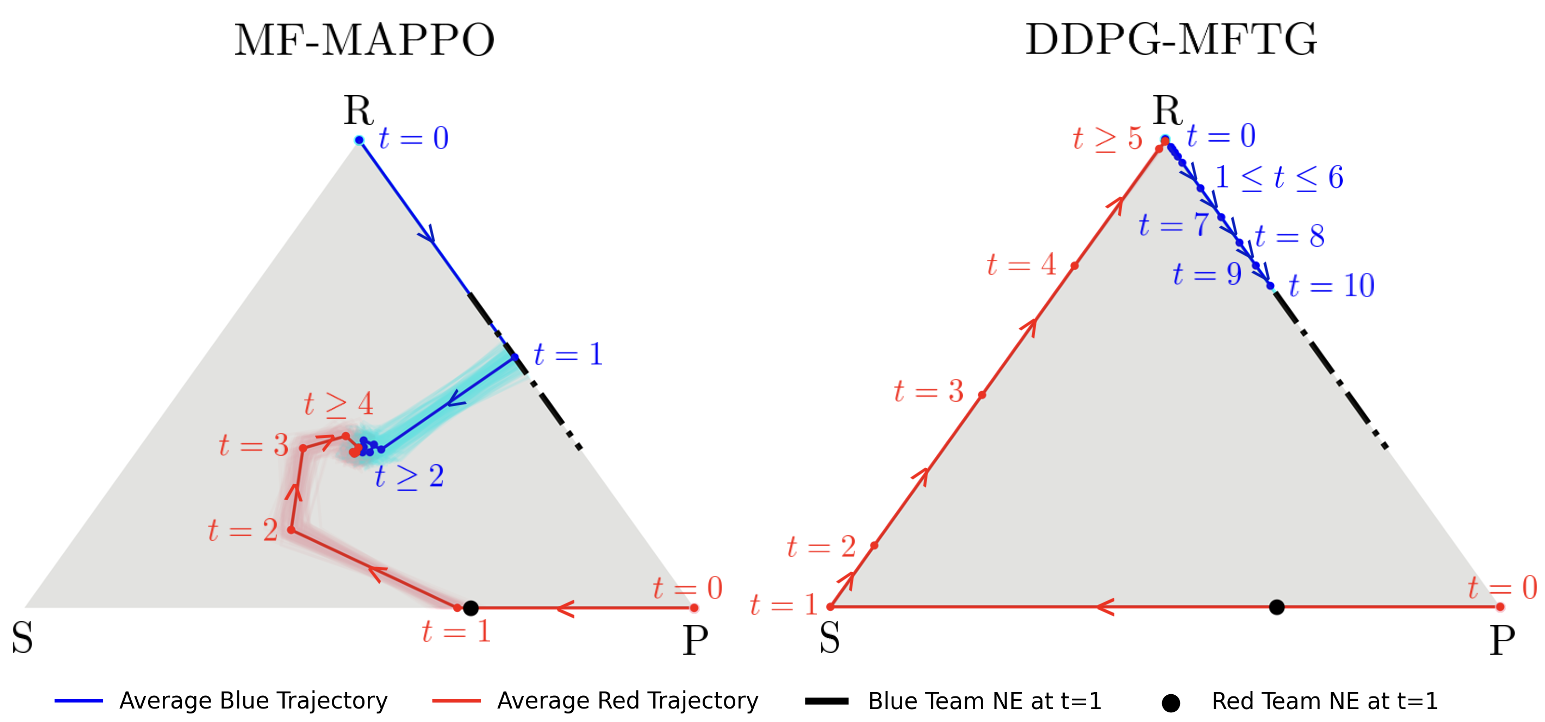
Figure 6. 150 initializations (cyan/pink) of $\mu_{t=0}=[1,0,0]^{\mbox{\tiny\sf T}}$ and $\nu_{t=0}=[0,1,0]^{\mbox{\tiny\sf T}}$ on a 3D simplex for cRPS for $N_{1}=N_{2}=1,000$.

Comparison of trajectories on a 3D simplex for cRPS using MF-MAPPO and DDPG-MFTG for 150 initializations.

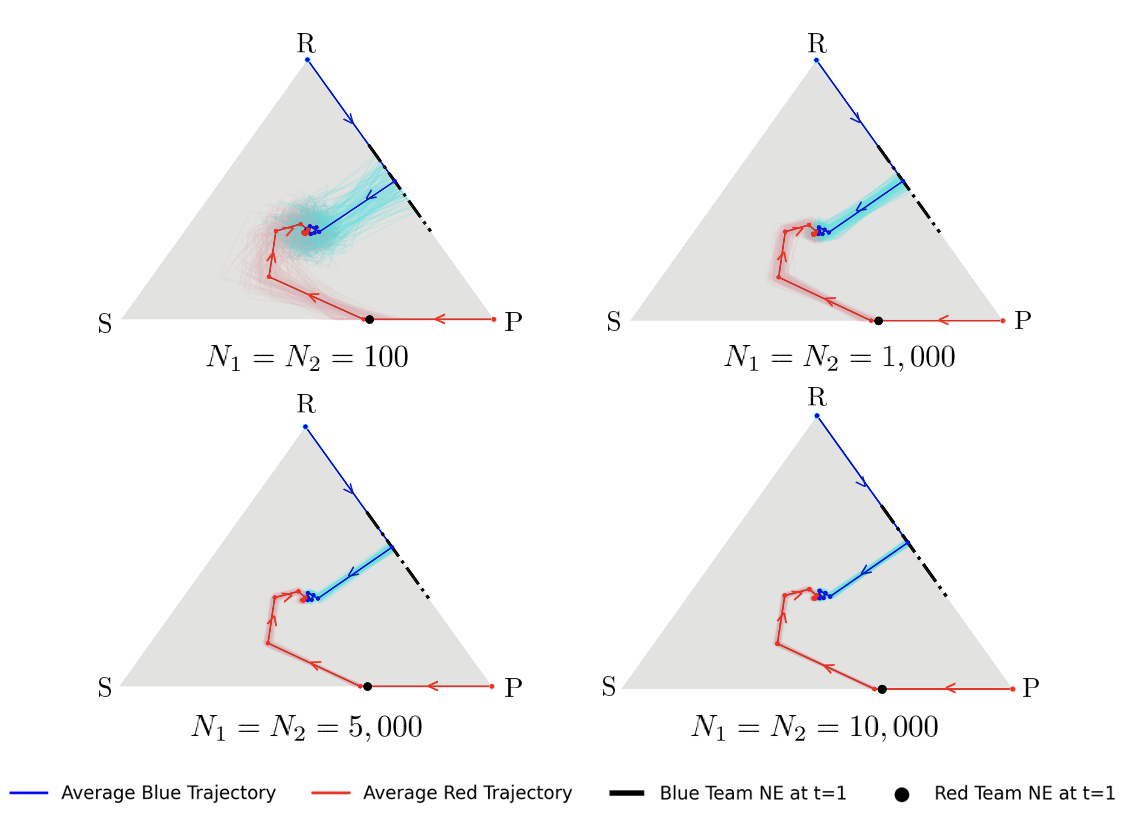
Figure 7. Deploying MF-MAPPO trained on $N_{1}=N_{2}=1,000$ to varying team sizes (150 trajectories) with the same initialization.

Deploying MF-MAPPO trained on $N_{1}=N_{2}=1,000$ to different population sizes for 150 initializations (cyan/pink)

Table 2. Performance Comparison for cRPS

Approach	Training Time	Average Reward	NE Attained?
MF-MAPPO	2h 17min 15s	-0.331	✓
DDPG-MFTG	60h 49min 41s	3.774	✗

These experiments show that MF-MAPPO learns stable policies that are consistent with the theoretical predictions, while DDPG-MFTG, despite its successes in Shao et al. (2024), struggles to stabilize in these simple ZS-MFTGs.

5.3. Battlefield Game

To fully test the capability of MF-MAPPO on a more complex scenario, we propose a battlefield game where an individual agent’s dynamics is highly coupled with both teams’ distributions.

We consider a large-scale two-team (Blue and Red) ZS-MFTG on an $n\times n$ grid world, modeling a target capture-type offense/defense scenario. The Blue agents aim to reach target locations without being deactivated, while the Red agents must learn to guard these targets. Each team can deactivate its opponents in a cell by maintaining numerical advantage over the opposing team at that cell. In all battlefield illustrations, the targets are shown in lilac color and the obstacles are shown in black; the bottom left cell is [0, 0].

5.3.1. Problem Setup and Objective.

The state of the $i^{th}$ Blue agent is defined as the pair $x_{i}=(p_{i}^{x},s_{i}^{x})$ where $p_{i}^{x}\in\mathcal{S}_{\text{position}}$ denotes the position of the agent in the grid world and $s_{i}^{x}\in\mathcal{S}_{\text{status}}=\{0,1\}$ defines the status of the agent: 0 being inactive and 1 being active. Similarly, we define the state of the Red agent as $y_{i}=(p_{i}^{y},s_{i}^{y})$. The state spaces for the Blue and Red teams are denoted by $\mathcal{X}=\mathcal{Y}=\mathcal{S}_{\text{position}}\times\mathcal{S}_{\text{status}}$, respectively. The mean-fields of the Blue ($\mu$) and Red ($\nu$) teams are distributions over the joint position and status space, i.e., ${\mu},{\nu}\in\mathcal{P}(\mathcal{S}_{\text{position}}\times\mathcal{S}_{\text{status}})$. The action spaces are given by $\mathcal{U}=\mathcal{V}=\{\texttt{Up},\texttt{Down},\texttt{Left},\texttt{Right},\texttt{Stay}\}$ for both teams, representing discrete movements in the grid world. The learned identical team policy assigns actions based on an agent’s local position and status, as well as the observed mean-fields of both teams.

An agent can be deactivated by the opponent with a nonzero probability if the opponent’s ED at the agent’s location exceeds that of the agent’s own team, which we refer to as the numerical advantage. The total transition probability from state $(p,s)$ to state $(p^{\prime},s^{\prime})$ by taking an action $a$ is given by

$$\mathbb{P}\big{(}(p^{\prime},s^{\prime})\,|\,(p,s),a,\mu,\nu\big{)}=\mathbb{P}\big{(}p^{\prime}\,|\,(p^{\prime},s^{\prime}),a\big{)}\,\mathbb{P}\big{(}s^{\prime}\,|\,(p,s),\mu,\nu\big{)},$$

where the first term on the right-hand side corresponds to the deterministic position transition when the agent is active. The second term corresponding to the status transition is given by

$$\mathbb{P}\big{(}0\mid(p,1),\mu,\nu\big{)} =\operatorname{clip}_{[0,1]}\big{(}\alpha_{x}(\nu(p)-\mu(p))\big{)},$$

$$\mathbb{P}\big{(}1\mid(p,1),\mu,\nu\big{)} =1-\mathbb{P}\big{(}0\mid(p,1),\mu,\nu\big{)},$$

where $\nu(p)-\mu(p)$ is the Red team’s numerical advantage over the Blue team at $p$, and $\alpha_{x}$ is a tuning parameter to control the Red team’s deactivation power. We can formulate a similar expression for the deactivation probability of the Red team based on the Blue team’s numerical advantage $\mu(p)-\nu(p)$.

These dynamics incentivize both teams to aggregate, i.e., to minimize the numerical advantage of the opponent team and ultimately reduce the risk of being deactivated. The Blue team’s reward depends on the fraction of agents active and at the target, and Red’s reward follows from the zero-sum structure. To avoid degeneracy, the Red agents are not allowed to enter the target.

5.3.2. Results and Discussion.

We conducted several experiments on various grid world maps with different target and obstacle layouts. In our experiments, we trained with $N_{1}=N_{2}=100$ agents and experimented with different initial distributions. Additional results are presented in the supplementary material.

Map 1:

A $4\times 4$ grid features a target partially obstructed by a diagonal obstacle (Figures 9-10). The Red team must position itself along left and the right corridors (cells [0, 2] and [1, 3]) to hinder Blue team’s advance. We compare MF-MAPPO and DDPG-MFTG by pitting them against each other in both offensive and defensive roles. As shown in Figure 8, MF-MAPPO consistently outperforms DDPG-MFTG across various initial positions, achieving up to $10\times$ higher rewards when attacking (Figures 8(a) and 8(c)). While both methods perform similarly in defense, visualizations reveal that DDPG-MFTG agents often fail to learn effective strategies, instead remaining stationary and aiming for a zero-reward outcome—an exploitable weakness.

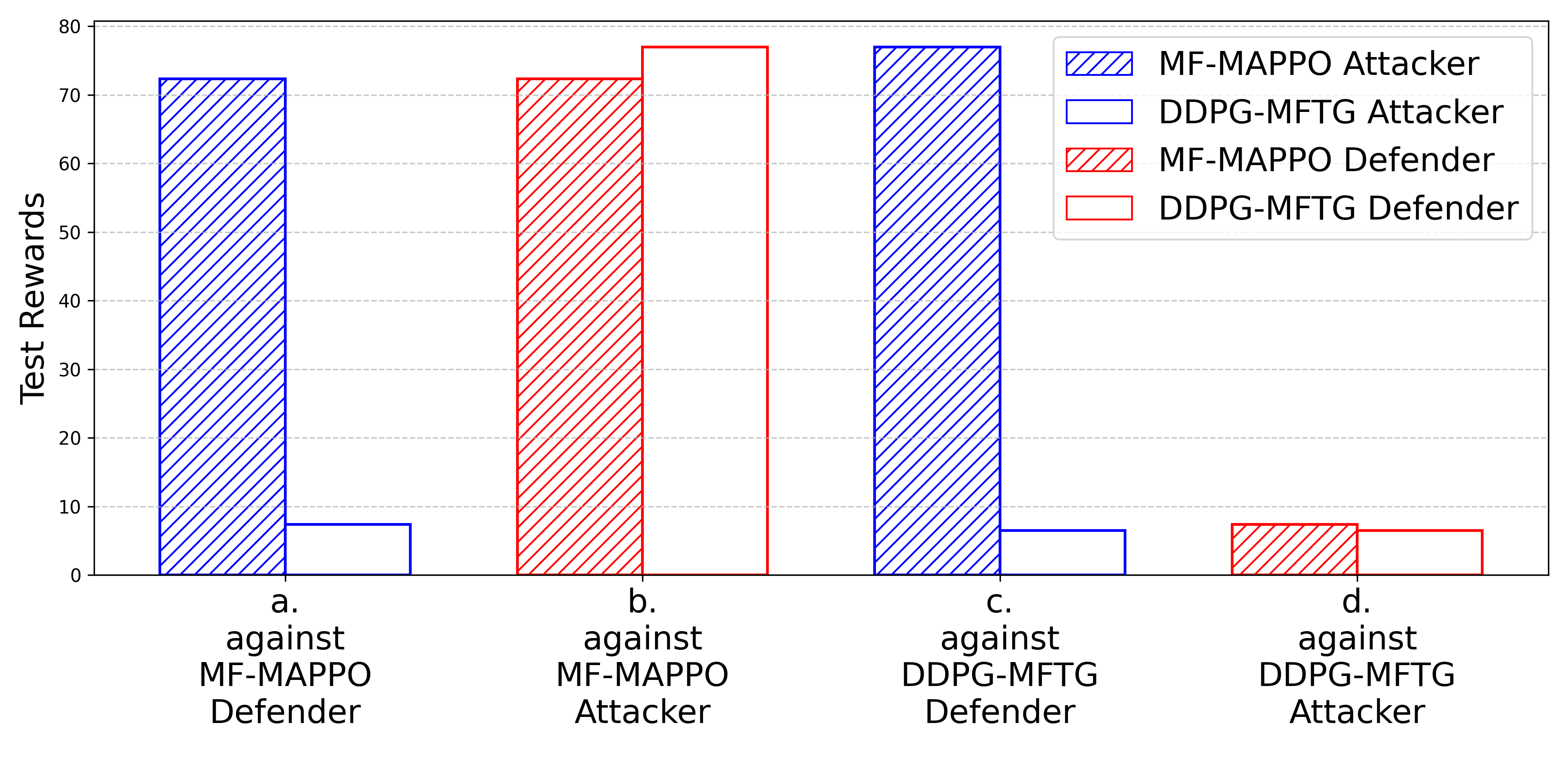
Figure 8. Average test rewards of MF-MAPPO vs. DDPG-MFTG on a 4x4 grid world for 100 random initializations.

Comparing MF-MAPPO with DDPG-MFTG on a 4x4 grid world for 100 random initial conditions.

Figure 9 compares the two algorithms against the baseline defending team. MF-MAPPO Blue agents exhibit coordinated maneuvering, forming coalitions to reach the target (a), whereas DDPG-MFTG Blue agents (b) show limited coordination, with only nearby agents reaching the target and distant agents failing to engage. Figure 9(c) represents MF-MAPPO vs. MF-MAPPO to illustrate the goal strategies and expected behavior.

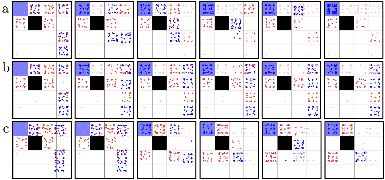
Figure 9. a. MF-MAPPO Blue vs. DDPG-MFTG Red; b. DDPG-MFTG Blue vs. DDPG-MFTG Red; c. MF-MAPPO Blue vs. MF-MAPPO Red.

a. MF-MAPPO Blue vs. DDPG-MFTG Red; b. DDPG-MFTG Blue vs. DDPG-MFTG Red; c. MF-MAPPO Blue vs. MF-MAPPO Red

We next evaluated MF-MAPPO’s performance as the Red defending team against the DDPG-MFTG Blue team (Figure 10). Due to the agents’ initial positions, the target entryway near [0, 2] remains unguarded, requiring the Red team to mobilize its agents to defend the area. MF-MAPPO Red agents successfully cover the entryway and deactivate several Blue attackers (a), whereas the DDPG-MFTG Red agents (b) fail to secure the second target. Moreover, (b) highlights that DDPG-MFTG Blue agents do not aggressively pursue the target, further illustrating their tendency to passively seek zero reward outcomes rather than take goal-directed actions, unlike (c).

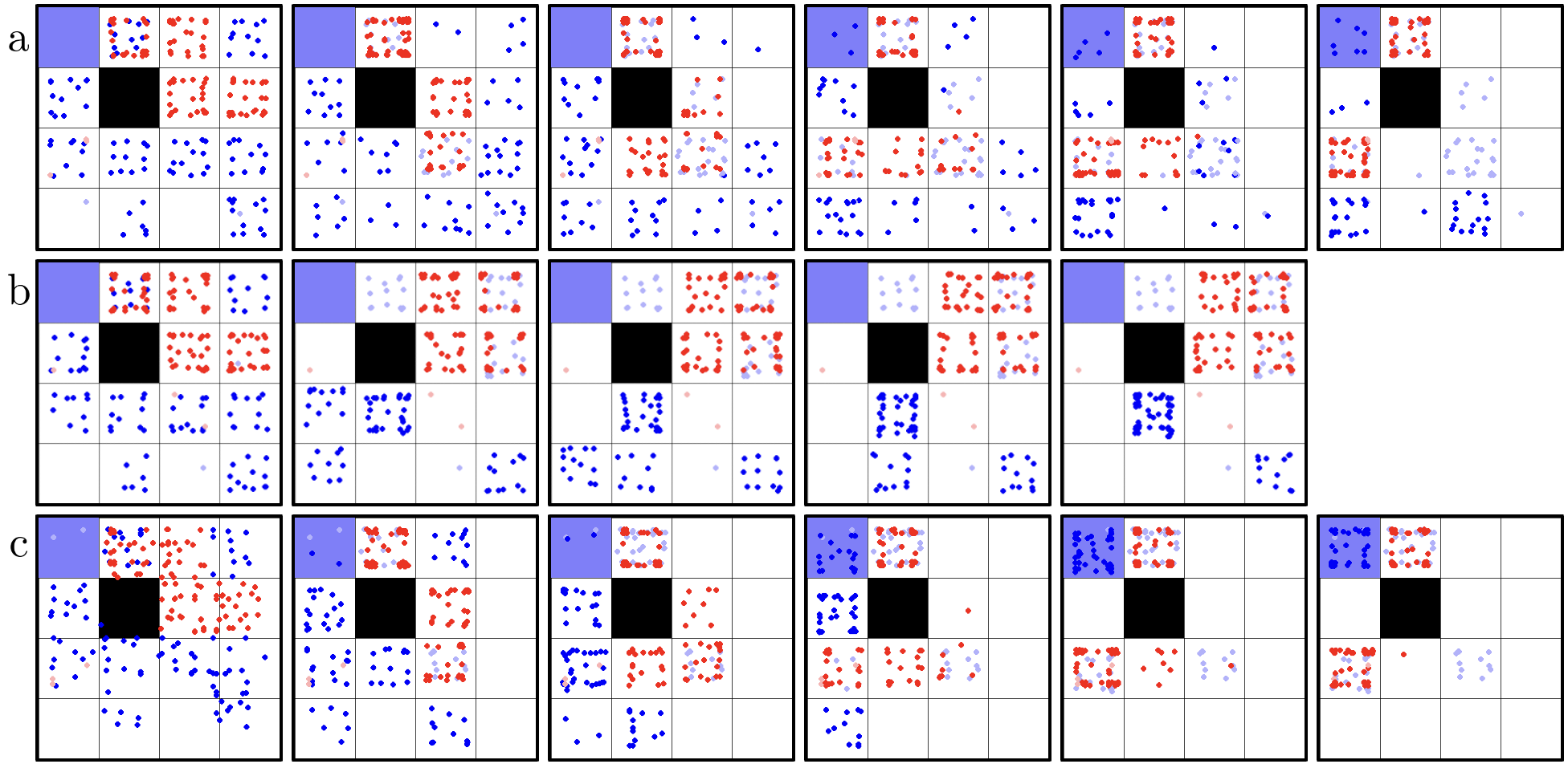
Figure 10. a. MF-MAPPO Red vs. DDPG-MFTG Blue; b. DDPG-MFTG Red vs. DDPG-MFTG Blue; c. MF-MAPPO Red vs. MF-MAPPO Blue.

a. MF-MAPPO Red vs. DDPG-MFTG Blue; b. DDPG-MFTG Red vs. DDPG-MFTG Blue; c. MF-MAPPO Red vs. MF-MAPPO Blue

Map 2:

We design a more complex $8\times 8$ grid with two targets (Figures 11 and 12). The Red team now faces a dilemma in determining which target to defend, while the Blue team must exploit this ambiguity to its advantage. Due to DDPG-MFTG’s high computational cost—which scales with the joint state-action space—and its high network update frequency, it is excluded from our analysis. In the absence of other baselines for such large scale complex games, we only qualitatively assess MF-MAPPO’s performance.

In Figure 11, the Red team is concentrated at one cell, while the Blue team is split: 30% at cell [1, 1] and the rest at cell [6, 6]. The Red team proceeds to deactivate the smaller group of Blue agents due to its numerical advantage. Upon seeing both the Blue groups advance towards the upper target, the Red team changes its trajectory in order to block the target as seen in (c). The Blue team then intelligently shifts toward the lower target, as assembling its forces there is more feasible than at the upper target, where the Red team maintains a strong presence (Figures 11(d)-11(g)).

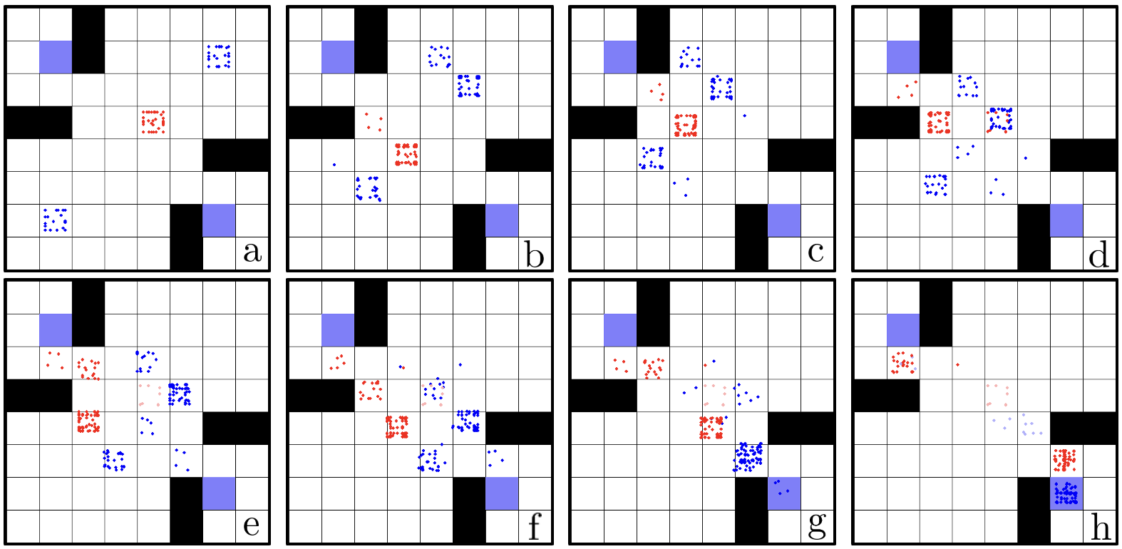
Figure 11. Red is concentrated; 30% Blue are at $[1,1]$ and the rest are at $[6,6]$.

MF-MAPPO Performance for Two Team Offense-Defense where Blue agents are attacking and Red are Defending Two Targets: Red is concentrated while 30% Blue are at $[1,1]$ and the rest are at $[6,6]$.

In Figure 12, the Blue team is evenly distributed across four cells, while the Red team is concentrated at [3, 3]. Blue agents move toward the nearest target, demonstrating heterogeneous behavior despite operating under an identical policy—highlighting the strength of the mean-field approximation. Similarly, the Red team also strategically divides to defend both targets its identical policy. Due to policy stochasticity and finite population effects, the split is uneven, prompting the upper Blue subgroup to redirect toward the lower target. This allows both lower Blue subgroups to reach their objective. The Red team quickly reallocates its agents in response and ultimately uses its numerical advantage to deactivate several Blue agents (Figure 12(h)).

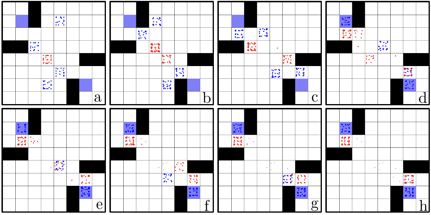
Figure 12. Blue is evenly split, Red is concentrated.

MF-MAPPO Performance for Two Team Offense-Defense where Blue agents are attacking and Red are Defending Two Targets: Blue agents are equally distributed among the four grid cells while Red is concentrated.

6. Conclusion

We introduced MF-MAPPO, a novel MARL algorithm for large-population competitive team games, leveraging finite mean-field approximation. Our design—featuring a minimally-informed critic and a shared team actor—achieves scalability without sacrificing performance. We evaluated MF-MAPPO against baselines like DDPG-MFTG on standard and constrained RPS, as well as a new MFTG battlefield scenario. Despite shared team policies, heterogeneous sub-population behaviors emerged, showing that mean-field approximations do not significantly limit performance. The battlefield testbed provides a rigorous benchmark for future research, supporting evaluations on accumulated rewards, sample efficiency, and computational complexity. A current limitation is that input dimensionality grows with the state space, which we aim to address through dimensionality reduction techniques (e.g., kernel embeddings).

This work was supported in part by ONR Award N00014-23-1-2308 and by ARL DCIST CRA W911NF-17-2-0181.

Appendix A Proof of Theoretical Results

A.1. Proof of Theorem 3.3

See 3.3 We have the following definition of the lower game value for the finite-population ZS-MFTG:

$$\underline{J}^{N*}(\mathbf{x}^{N_{1}},\mathbf{y}^{N_{2}})=\max_{\mathbf{\phi}^{N_{1}}\in\Phi^{N_{1}}}\min_{\mathbf{\psi}^{N_{2}}\in\Psi^{N_{2}}}J^{N,\phi^{N_{1}},\psi^{N_{2}}}(\mathbf{x}^{N_{1}},\mathbf{y}^{N_{2}}).$$ (A.1)

Note that the maximization for the Blue team is being performed over the set of all team policies $\Phi^{N_{1}}$, including identical as well non-identical team policies. If we restrict ourselves to the set of identical team policies $\Phi\subseteq\Phi^{N_{1}}$ it follows immediately that

$$\underline{J}^{N*}(\mathbf{x}^{N_{1}},\mathbf{y}^{N_{2}})\geq\max_{\mathbf{\phi}^{N_{1}}\in\Phi}\min_{\mathbf{\psi}^{N_{2}}\in\Psi^{N_{2}}}J^{N,\phi^{N_{1}},\psi^{N_{2}}}(\mathbf{x}^{N_{1}},\mathbf{y}^{N_{2}}).$$ (A.2)

Suppose that $\phi^{*}_{\mathrm{finite}}$ is the optimal identical Blue team policy obtained from the finite population game. It follows from (A.1) that

$$\underline{J}^{N*}(\mathbf{x}^{N_{1}},\mathbf{y}^{N_{2}})\geq\min_{\psi^{N_{2}}\in\Psi^{N_{2}}}J^{N,\phi^{*}_{\mathrm{finite}},\psi^{N_{2}}}(\mathbf{x}^{N_{1}},\mathbf{y}^{N_{2}}).$$ (A.3)

Furthermore, let $\phi^{*}\in\Phi$ be the optimal identical Blue team policy obtained from the equivalent zero-sum (infinite-population) coordinator game and

$$\min_{\mathbf{\psi}^{N_{2}}\in\Psi^{N_{2}}}J^{N,\phi^{*}_{\mathrm{finite}},\psi^{N_{2}}}(\mathbf{x}^{N_{1}},\mathbf{y}^{N_{2}})\geq\min_{\psi^{N_{2}}\in\Psi^{N_{2}}}J^{N,\phi^{*},\psi^{N_{2}}}(\mathbf{x}^{N_{1}},\mathbf{y}^{N_{2}}).$$ (A.4)

Using Theorem 3.3, and using (A.4), yields

$$\underline{J}^{N*}(\mathbf{x}^{N_{1}},\mathbf{y}^{N_{2}}) \geq\min_{\psi^{N_{2}}\in\Psi^{N_{2}}}J^{N,\phi^{*}_{\mathrm{finite}},\psi^{N_{2}}}(\mathbf{x}^{N_{1}},\mathbf{y}^{N_{2}})$$

$$\geq\min_{\psi^{N_{2}}\in\Psi^{N_{2}}}J^{N,\phi^{*},\psi^{N_{2}}}(\mathbf{x}^{N_{1}},\mathbf{y}^{N_{2}})$$

$$\geq\underline{J}^{N*}(\mathbf{x}^{N_{1}},\mathbf{y}^{N_{2}})-\mathcal{O}\Big{(}\frac{1}{\sqrt{\underline{N}}}\Big{)},$$

where $\underline{N}=\min\{N_{1},N_{2}\}$. Upon rearranging terms, we finally have,

$$\min_{\psi^{N_{2}}\in\Psi^{N_{2}}}J^{N,\phi^{*}_{\mathrm{finite}},\psi^{N_{2}}}(\mathbf{x}^{N_{1}},\mathbf{y}^{N_{2}})-\min_{\psi^{N_{2}}\in\Psi^{N_{2}}}J^{N,\phi^{*},\psi^{N_{2}}}(\mathbf{x}^{N_{1}},\mathbf{y}^{N_{2}})\leq\epsilon,$$

where $\epsilon=\mathcal{O}({1}/{\sqrt{\underline{N}}})$ .

A.2. Proof of Proposition 5.2

See 5.2 For the constrained RPS game under the stated initial condition, we cannot obtain the target distribution $\begin{bmatrix}\frac{1}{3}&\frac{1}{3}&\frac{1}{3}\end{bmatrix}^{\mbox{\tiny\sf T}}$ after a single time step but this may be possible for $t\geq 2$. To this end, consider the following candidate trajectory respecting the transition dynamics:

$${\mu}_{0}^{\mbox{\tiny\sf T}} =\begin{bmatrix}1&0&0\end{bmatrix},$$

$${\mu}_{1}^{\mbox{\tiny\sf T}} =\begin{bmatrix}1-x_{1}&x_{1}&0\end{bmatrix},$$

$${\mu}_{2}^{\mbox{\tiny\sf T}} =\begin{bmatrix}1-x_{1}-x_{2}&x_{1}+x_{2}-x_{3}&x_{3}\end{bmatrix},$$

$${\mu}_{t}^{\mbox{\tiny\sf T}} =\begin{bmatrix}\frac{1}{3}&\frac{1}{3}&\frac{1}{3}\end{bmatrix},\quad\forall t>2.$$

$${\nu}_{0}^{\mbox{\tiny\sf T}} =\begin{bmatrix}0&1&0\end{bmatrix},$$

$${\nu}_{1}^{\mbox{\tiny\sf T}} =\begin{bmatrix}0&1-y_{1}&y_{1}\end{bmatrix},$$

$${\nu}_{2}^{\mbox{\tiny\sf T}} =\begin{bmatrix}y_{3}&1-y_{1}-y_{2}&y_{1}+y_{2}-y_{3}\end{bmatrix},$$

$${\nu}_{t}^{\mbox{\tiny\sf T}} =\begin{bmatrix}\frac{1}{3}&\frac{1}{3}&\frac{1}{3}\end{bmatrix},\quad\forall t>2.$$

In order to respect the simplex structure for ${\mu}_{t}$ and ${\nu}_{t}$, we have the following constraints at all times:

$$0\leq x_{1},x_{2},x_{3}\leq 1,\quad x_{2}\leq 1-x_{1},\quad x_{3}\leq x_{1}.$$

Similarly,

$$0\leq y_{1},y_{2},y_{3}\leq 1,\quad y_{2}\leq 1-y_{1},\quad y_{3}\leq y_{1}.$$

For the distribution at $t=2$ to be $\begin{bmatrix}\frac{1}{3}&\frac{1}{3}&\frac{1}{3}\end{bmatrix}^{\mbox{\tiny\sf T}}$ for both teams, we get the additional constraints

$$x_{3}=y_{3}=\frac{1}{3},$$

$$x_{1}+x_{2}-x_{3}=y_{1}+y_{2}-y_{3}=\frac{1}{3},$$

$$\Rightarrow x_{1}+x_{2}=y_{1}+y_{2}=\frac{2}{3},$$

which implies that

$$x_{1},y_{1}\leq\frac{2}{3},$$

since $x_{2},y_{2}\geq 0$. The constraints now take the form

$$\frac{1}{3} \leq x_{1}\leq\frac{2}{3},$$ (A.5)

and similarly,

$$\frac{1}{3} \leq y_{1}\leq\frac{2}{3}.$$ (A.6)

The objective function for cRPS is given by

$$J^{N,\phi,\psi}\big{(}\mu_{0},\nu_{0}\big{)}=\mathbb{E}_{{\phi,\psi}}\!\Big{[}\sum_{t=1}^{T}\mu_{t}^{\mbox{\tiny\sf T}}A\nu_{t}\Big{|}\mu_{0},\nu_{0}\Big{]},$$ (A.7)

which leads to the optimization problem

$$\begin{array}[]{rrclcl}\displaystyle\max_{{\phi}^{t}}\min_{{\psi}^{t}}&\lx@intercol J^{N_{1},N_{2},{\phi}^{t},{\psi}^{t}}({\mu}_{0},{\nu}_{0})={\mu}_{1}^{\mbox{\tiny\sf T}}A{\nu}_{1}\hfil\lx@intercol.\end{array}$$ (A.8)

Substituting $\mu_{1}^{\mbox{\tiny\sf T}}=[1-x_{1},x_{1},0]$ and $\nu_{1}^{\mbox{\tiny\sf T}}=[0,1-y_{1},y_{1}]$ results in the following expression for the maximizing Blue team:

$$\max_{{\phi}^{t}}\quad J^{N_{1},N_{2},{\phi}^{t},{\psi}^{t}}({\mu}_{0},{\nu}_{0}) =x_{1}+2y_{1}-3x_{1}y_{1}-1$$

$$=x_{1}(1-3y_{1})+(2y_{1}-1).$$

Since this equation is linear in $x_{1}$, the solution to the maximization problem subject to the constraint (A.5) is

$$x_{1}=\frac{1}{3},\quad y_{1}>\frac{1}{3},$$ (A.9)

$$x_{1}=\frac{2}{3},\quad y_{1}<\frac{1}{3},$$ (A.10)

$$x_{1}\in[\frac{1}{3},\frac{2}{3}],\quad y_{1}=\frac{1}{3}.$$ (A.11)

Following the same approach for the minimizing Red team, we get the following objective,

$$\min_{{\psi}^{t}}\quad J^{N_{1},N_{2},{\phi}^{t},{\psi}^{t}}({\mu}_{0},{\nu}_{0}) =x_{1}+2y_{1}-3x_{1}y_{1}-1$$

$$=y_{1}(2-3x_{1})+(x_{1}-1),$$

subject to the constraint (A.6), with the solution being:

$$y_{1}=\frac{1}{3},\quad x_{1}<\frac{2}{3},$$ (A.12)

$$y_{1}=\frac{2}{3},\quad x_{1}>\frac{2}{3},$$ (A.13)

$$y_{1}\in[\frac{1}{3},\frac{2}{3}],\quad x_{1}=\frac{2}{3}.$$ (A.14)

Constraint (A.5) ensures that (A.13) cannot hold, while constraint (A.6) similarly prevents (A.10) from holding.

Consider now the case when $y_{1}>\frac{1}{3}$. From (A.9) it follows that $x_{1}=\frac{1}{3}$. Conversely, if the Blue team commits to a distribution with $x_{1}=\frac{1}{3}$, the Red team’s best response given by (A.12) gives $y_{1}=\frac{1}{3}$, resulting in an incentive for the Red team to deviate from $y_{1}>\frac{1}{3}$. Thus, (A.9) does not constitute an optimal solution. Following a similar argument, it can be shown that (A.14) is not an optimal solution either, as illustrated below.

Assume that $x_{1}=\frac{2}{3}$. From (A.14), $y_{1}\in[\frac{1}{3},\frac{2}{3}]$. Now, if the Red team announces that it will deploy the distribution $y_{1}\in[\frac{1}{3},\frac{2}{3}]$, the Blue team’s response for $x_{1}$ follows from (A.9) and (A.11). We have already established that (A.9) is not an optimal solution. This implies that $x_{1}\in[\frac{1}{3},\frac{2}{3}]$ can be a possible response to the Red team. However it violates (A.14), where $x_{1}=\frac{2}{3}$ follows from strict equality. Thus, (A.14) does not constitute an optimal solution as the Blue team has an incentive to deviate.

Now, suppose the Blue team announces a distribution where $x_{1}\in[\frac{1}{3},\frac{2}{3}]$. In this case, the Red team’s optimal response, derived from (A.12) and (A.11), is $y_{1}=\frac{1}{3}$. Conversely, if the Red team announces that its distribution will be $y_{1}=\frac{1}{3}$, the Blue team will still follow $x_{1}\in[\frac{1}{3},\frac{2}{3}]$. Since neither team has an incentive to deviate from these distributions, they form an optimal trajectory. Thus, the solution to the bilinear optimization problem for two-time step convergence takes the form:

$${\mu}^{*}_{1}=\begin{bmatrix}1-x_{1}\\ x_{1}\\ 0\end{bmatrix}\quad\text{and}\quad{\nu}^{*}_{1}=\begin{bmatrix}0\\[3.0pt] \frac{2}{3}\\[3.0pt] \frac{1}{3}\end{bmatrix},$$ (A.15)

such that $x_{1}\in[\frac{1}{3},\frac{2}{3}]$, leading to a game value of $-\frac{1}{3}$. This establishes the distribution at $t=1$ and confirms the existence of a two-time step optimal trajectory, thereby proving the first part of the proposition.

Now note the following:

1. The original objective function (A.7) can be expressed in a bilinear form (similar to the expressions for $\mu_{0},\mu_{1},\mu_{2}$ using $x_{1},x_{2},x_{3}$). This makes it concave in the first argument and convex in the second argument.

2. The mean-fields $\mu$ and $\nu$ lie on a simplex and are hence, compact and convex.

Thus, by the generalized version of von Neumann’s minimax theorem Sorin (2002), we conclude that the game value is unique, proving the second part of the proposition .

Appendix B RPS and cRPS Setup

B.1. State Space

We have three states in this representation of the game: rock, paper and scissors. We denote this state space as $\mathcal{S}=\{\texttt{R,P,S}\}$. The empirical distribution of the Blue team is denoted by ${\mu}\in\mathcal{P(S)}$ and that of the Red team is denoted by ${\nu}\in\mathcal{P(S)}$. Since we have three states for each team, both EDs lie in a three-dimensional simplex denoted by $\mathcal{P(S)}$.

B.2. Action Space

B.2.1. RPS

At each state, we define three actions denoted by $\mathcal{A}=\{\texttt{CW},\texttt{CCW},\texttt{Stay}\}$. These actions represent the ability of the agents to move from one state to the other in the following fashion:

1. CW denotes a clockwise cyclic action from one state to the other, i.e., from $\texttt{R}\rightarrow\texttt{P}$, $\texttt{P}\rightarrow\texttt{S}$, $\texttt{S}\rightarrow\texttt{R}$.

2. CCW denotes a counterclockwise cyclic movement, i.e., from $\texttt{R}\rightarrow\texttt{S}$, $\texttt{S}\rightarrow\texttt{P}$, $\texttt{P}\rightarrow\texttt{R}$.

3. Stay denotes the idle action (remain in the same state as before).

B.2.2. cRPS

At each state we have two actions denoted by $\mathcal{A}=\{\texttt{CW},\texttt{Stay}\}$. These actions represent the ability of the agents to move from one state to the other in the following fashion:

1. CW denotes a clockwise cyclic action from one state to the other, i.e., from $\texttt{R}\rightarrow\texttt{P}$, $\texttt{P}\rightarrow\texttt{S}$, $\texttt{S}\rightarrow\texttt{R}$.

2. Stay denotes the idle action (remain in the same state as before).

Thus, we cannot directly jump from R to S within a single step, but must go via P. Mathematically, S does not lie in the reachable set of R. The reachable set $\mathcal{R}(s)$ for each state $s$ at a given time step under this modified action space is as follows

$$\mathcal{R}(\texttt{R})=\{\texttt{R},\texttt{P}\},\quad\mathcal{R}(\texttt{P})=\{\texttt{P},\texttt{S}\},\quad\mathcal{R}(\texttt{S})=\{\texttt{S},\texttt{R}\}.$$

B.3. Dynamics and Transition Probabilities

For both RPS and cRPS, we consider deterministic transitions $\mathcal{T}(s,a,s^{\prime})$, which implies that given a state-action pair $(s,a)$, the agent reaches a unique next state $s^{\prime}$ with certainty (no distribution over the reachable states). Thus, for state R and action Stay, the transition function $\mathcal{T}:\mathcal{S}\times\mathcal{A}\times\mathcal{S}\rightarrow\{0,1\}$ is given as:

$$\mathcal{T}(\texttt{R},\texttt{Stay},\texttt{R})=1,\quad\mathcal{T}(\texttt{R},\texttt{Stay},\texttt{P})=0,\quad\mathcal{T}(\texttt{R},\texttt{Stay},\texttt{S})=0.$$

This implies that an agent in the state R upon taking the Stay action remains in state R. Similarly,

$$\mathcal{T}(\texttt{R},\texttt{CW},\texttt{R})=0,\quad\mathcal{T}(\texttt{R},\texttt{CW},\texttt{P})=1,\quad\mathcal{T}(\texttt{R},\texttt{CW},\texttt{S})=0.$$

represent the method to transition from R to P .

B.4. Reward Structure

In a two player RPS game, the reward matrix for Player 1 is defined as:

$$A=\begin{bmatrix}\begin{array}[]{rrr}0&-1&1\\ 1&0&-1\\ -1&1&0\end{array}\end{bmatrix}.$$

We extend this two-player framework to the multi-agent team game formulation. Define the pairwise reward for an agent at state $x\in\mathcal{S}$ within the Blue team and at state $y\in\mathcal{S}$ from the Red team as

$$r(x,y)\triangleq A_{xy},$$

where $A_{xy}$ represents the element from the reward matrix $A$ corresponding to the states $x$ (row player) and $y$ (column player). In lieu of the zero-sum structure, the reward for the agent at $y$ with respect to $x$ becomes $-r(x,y)$. Thus, for each player $x_{i}\in\mathcal{S}\text{ and }i=1,2,\ldots,N_{1}$ in the Blue team and $y_{j}\in\mathcal{S}\text{ and }j=1,2,\ldots,N_{2}$ in the Red team, the reward for the Blue team can be defined as

$$R_{\mathrm{Blue}}(\mathbf{x},\mathbf{y})=\frac{1}{N_{1}}\sum_{i=1}^{N_{1}}\underbrace{\Big{[}\frac{1}{N_{2}}\sum_{j=1}^{N_{2}}r(x_{i},y_{j})\Big{]}}_{\text{reward for agent $i$}}.$$

Rewriting the term inside the square brackets as

$$\frac{1}{N_{2}}\sum_{j=1}^{N_{2}}r(x_{i},y_{j}) =\frac{1}{N_{2}}\sum_{y\in\mathcal{S}}\sum_{j=1}^{N_{2}}r(x_{i},y)\mathbf{1}_{y_{j}=y}$$

$$=A_{x_{i}s_{0}}\sum_{j=1}^{N_{2}}\frac{1}{N_{2}}\mathbf{1}_{y_{j}=s_{0}}+A_{x_{i}s_{1}}\sum_{j=1}^{N_{2}}\frac{1}{N_{2}}\mathbf{1}_{y_{j}=s_{1}}$$

$$+A_{x_{i}s_{2}}\sum_{j=1}^{N_{2}}\frac{1}{N_{2}}\mathbf{1}_{y_{j}=s_{2}}$$

$$=A_{x_{i}s_{0}}{\nu}(s_{0})+A_{x_{i}s_{1}}{\nu}(s_{1})+A_{x_{i}s_{2}}{\nu}(s_{2})$$

$$=A(x_{i}){\nu},$$ (B.16)

where $A(x_{i})$ is the row of the reward matrix corresponding to state $x_{i}$. Using (B.4), the total Blue reward can be expressed as

$$R_{\mathrm{Blue}}(\mathbf{x},\mathbf{y}) =\frac{1}{N_{1}}\sum_{i=1}^{N_{1}}A(x_{i}){\nu}$$

$$=\Bigl{(}\frac{1}{N_{1}}\sum_{x\in\mathcal{S}}\sum_{i=1}^{N_{1}}A(x_{i})\mathbf{1}_{x_{i}=x}\Bigr{)}{\nu}$$

$$=\Bigl{(}A(s_{0}){\mu}(s_{0})+A(s_{1}){\mu}(s_{1})+A(s_{2}){\mu}(s_{2})\Bigr{)}{\nu}$$

$$={\mu}^{\mbox{\tiny\sf T}}A{\nu}.$$

B.5. Implementation Details and Hyperparameters

The state distributions are represented as arrays that are concatenated together to form the global observation. This becomes the input to the critic network which consists of a single hidden layer of 64 neurons and two tanh activation functions. The output is a single value that is equal to the estimated value function. On the other hand, the actor-network consists of a single MLP layer of 64 neurons that is concatenated with the local agent observation. Additionally, the logits are converted to a probability distribution through a softmax layer. The dimension scales with $|\mathcal{A}|$. Both the actor and critic networks are initialized using orthogonal initialization (Huang et al., 2022).

The single-stage RPS game is trained for 5,000 time steps with the actor and critic learning rates set to 0.0005 and 0.001, respectively, which remain constant throughout training. The networks are updated using the ADAM optimizer Kingma and Ba (2017) every 50 time steps for 10 epochs and a PPO clip value of 0.1. The entropy is decayed from 0.01 to 0.001 geometrically. We use an episode length of 1 after which the rewards are bootstrapped.

Moreover, since we have a single “team” buffer and the input/output dimensions are small, we do not use a mini-batch based update. For cRPS we use an episode length of 10 after which the rewards are bootstrapped. cRPS is trained using 200,000 time steps (=20,000 episodes) and is updated every 100 time steps. The algorithm was trained on a single NVIDIA GeForce RTX 3070 GPU and the training times are given in Tables 1 and 2.

Appendix C Battlefield Setup

C.1. State and Action Space

We consider a large-scale two-team (Blue and Red) ZS-MFTG on an $n\times n$ grid world. The state of the $i^{th}$ Blue agent is defined as the pair $x_{i}=(p_{i}^{x},s_{i}^{x})$ where $p_{i}^{x}\in\mathcal{S}_{\text{position}}$ denotes the position of the agent in the grid world and $s_{i}^{x}\in\mathcal{S}_{\text{status}}=\{0,1\}$ defines the status of the agent: 0 being inactive and 1 being active. Similarly, we define the state of the Red agent as $y_{i}=(p_{i}^{y},s_{i}^{y})$. The state spaces for the Blue and Red teams are denoted by $\mathcal{X}=\mathcal{Y}=\mathcal{S}_{\text{position}}\times\mathcal{S}_{\text{status}}$, respectively. The mean-fields of the Blue ($\mu$) and Red ($\nu$) teams are distributions over the joint position and status space, i.e., ${\mu},{\nu}\in\mathcal{P}(\mathcal{S}_{\text{position}}\times\mathcal{S}_{\text{status}})$. The action spaces are given by $\mathcal{U}=\mathcal{V}=\{\texttt{Up},\texttt{Down},\texttt{Left},\texttt{Right},\texttt{Stay}\}$ for both teams, representing discrete movements in the grid world. The learned identical team policy assigns actions based on an agent’s local position and status, as well as the observed mean-fields of both teams. In the following subsections, we elaborate on the weakly coupled transition dynamics and reward structure introduced in the game, followed by a detailed discussion of the training procedure and network architecture for MF-MAPPO in this example.

C.2. Interaction Between Agents

The transitions between states for agents belonging to both teams are characterized by their dynamics. These dynamics are probabilistic and depend on interactions among agents and are weakly coupled through their mean-field distributions. The weak coupling dynamics is keeping in line with the assumption in Guan et al. (2024).

An agent at a given grid cell can be deactivated by the opponent team with a nonzero probability if the empirical mean-field of the opponent team at the grid cell supersedes that of the agent’s own team. Similarly, a deactivated agent can be revived if the empirical mean-field of the agent’s team is greater than the opponent’s. This is referred to as numerical advantage.

The total transition probability from a state $(p,s)$ to $(p^{\prime},s^{\prime})$ by taking an action $a$ is given by the product of transitioning from $(p^{\prime}|(p,s),a,\mu,\nu)$ and $(s^{\prime}|(p,s),a,\mu,\nu)$. For simplicity, we consider that the position transition does not depend on the mean-field and the status transition does not depend on the action taken. For agent $i$ belonging to the Blue team, the expression is formulated as

$$\mathbb{P}\big{(}x_{i}^{\prime}\,|\,x_{i},a_{i},\mu,\nu\big{)} =\mathbb{P}\big{(}(p_{i}^{x^{\prime}},s_{i}^{x^{\prime}})\,|\,(p_{i}^{x},s_{i}^{x}),a_{i},\mu,\nu\big{)}$$

$$=\mathbb{P}\big{(}p_{i}^{x^{\prime}}\,|\,(p_{i}^{x},s_{i}^{x}),a_{i}\big{)}\mathbb{P}\big{(}s_{i}^{x^{\prime}}\,|\,(p_{i}^{x},s_{i}^{x}),\mu,\nu\big{)}.$$

Here, $\mathbb{P}\big{(}p_{i}^{x^{\prime}}\,|\,(p_{i}^{x},s_{i}^{x}),a_{i}\big{)}$ is given by

$$\mathbb{P}\big{(}p_{i}^{x^{\prime}}\,|\,(p_{i}^{x},s_{i}^{x}),a_{i}\big{)}=\begin{cases}1,\quad&s_{i}^{x}=1\text{ and no boundary}\\ 0,\quad&\text{otherwise}.\end{cases}$$

Calculating $\mathbb{P}\big{(}s_{i}^{x^{\prime}}\,|\,(p_{i}^{x},s_{i}^{x}),\mu,\nu\big{)}$ yields

$$\mathbb{P}\big{(}1\,|\,(p_{i}^{x},1),\mu,\nu\big{)} =1-\alpha_{x}\big{(}\nu(p_{i}^{x})-\mu(p_{i}^{x})\big{)},$$

$$\mathbb{P}\big{(}0\,|\,(p_{i}^{x},1),\mu,\nu\big{)} =\alpha_{x}\big{(}\nu(p_{i}^{x})-\mu(p_{i}^{x})\big{)},$$

and

$$\mathbb{P}\big{(}1\,|\,(p_{i}^{x},0),\mu,\nu\big{)} =\beta_{x}\big{(}\mu(p_{i}^{x})-\nu(p_{i}^{x})\big{)},$$

$$\mathbb{P}\big{(}0\,|\,(p_{i}^{x},0),\mu,\nu\big{)} =1-\beta_{x}\big{(}\mu(p_{i}^{x})-\nu(p_{i}^{x})\big{)},$$

where $\alpha_{x}$ and $\beta_{x}$ are parameters that control the amount of activation and deactivation and $\big{(}\nu(p_{i}^{x})-\mu(p_{i}^{x})\big{)}$ and $\big{(}\mu(p_{i}^{x})-\nu(p_{i}^{x})\big{)}$ are the numerical advantages of the Red (over Blue) and Blue (over red) teams at position $p^{x}$ respectively. The values are clipped between $0$ and $1$. The Red team, being the defending team, is given a slight advantage in terms of higher deactivation power. This enables the possibility of capturing Blue team agents. However, to avoid degeneracy, the Red team agents are not allowed to penetrate the target , that is,

$$\mathbb{P}\big{(}(p_{i}^{y^{\prime}}=\text{Target})\,|\,(p_{i}^{y},s_{i}^{y}),v_{i}\big{)} =0\quad p_{i}^{y}\neq\text{Target}.$$

For our experiments, we assume $\alpha_{x}=15$, $\alpha_{y}=5$, and $\beta_{x}=\beta_{y}=0.$

C.3. Reward Structure

The team rewards only depend on the mean-fields of the two teams. For the battlefield scenario, the Blue team agents receive a positive reward corresponding to the fraction of agents that reach the target alive. This is a one-time reward that depends on the change in the fraction of the population of the agents at the target, i.e., if ${\mu}_{t}|_{\text{target}}={\mu}_{t+1}|_{\text{target}}$, then the team does not receive any positive reward. Each agent in the team receives an identical “team reward.” The reward function is mathematically formulated as

$$R_{\text{Blue},{t+1}}(\mu,\nu)=\kappa\,\Delta\mu_{t+1}|_{\text{target}},$$

where,

$$\Delta\mu_{t+1}|_{\text{target}} =\mu_{t+1}(p^{x}=\text{Target},s^{x}=1)-\mu_{t}(p^{x}=\text{Target},s^{x}=1).$$

We have chosen $\kappa=100$ in our simulations (heavier emphasis on reaching the target). The Red team’s reward is the negative of the Blue team since we have a zero-sum game. Each team aims to maximize its own expected reward.

C.4. Implementation and Hyperparameters

The state distribution for a grid world of size $n\times n$ is represented as a three-dimensional array of size $(2,n,n)$ for each team. The first layer depicts the mean-field of the agents over an $n\times n$ grid that are alive and active, while the second layer gives information about the team’s deactivated population. Each team’s distribution is then concatenated together to form the global observation. This becomes the common information that is the input to the critic network which in our case is of size $(4,n,n)$ as we have two teams. Both neural networks consist of two main parts: a convolutional block and a fully connected block.

For the critic, the first CNN layer is the input layer that takes the 4 channels and outputs 32 channels, with a kernel size of 3x3, stride of 1, and padding of 1. Followed by ReLU activation, we have a hidden layer that takes 32 channels and outputs 64 channels, with the same kernel size, stride, and padding. Lastly, after another ReLU activation, we have the output layer that takes 64 channels and outputs 64 channels, again with the same kernel size, stride, and padding. After another ReLU layer, the output of the CNN is passed through an MLP. Namely, a fully connected (dense) layer takes the flattened output of the convolutional block and reduces it to 128 units. Between the input and the output layers, we have a single tanh activation function.

On the other hand, the input to the actor-network is split into two CNN blocks: one to process the common information and one to process the local information. The local information channel, is an array of size $(1,n,n)$ that locates the position of the agent with value +1 if it is active and -1 if it has been deactivated. This local information is passed through a single CNN layer that outputs 16 channels with a kernel size of 3x3, stride of 1, and padding of 1 while the common information is passed through two such layers with the output of 32 channels. Both outputs are then followed by a ReLU activation function and the latent representation of the common information combined with the local agent observation is then passed through an MLP architecture.

A fully connected (dense) layer takes the flattened output of the convolutional block and reduces it to 512 units. We have a single hidden layer that reduces the dimension further to 128 and then the output logits. The layers are separated by the tanh activation functions. Finally, the logits are converted to a probability distribution through a softmax layer. Both the actor and critic networks are initialized using orthogonal initialization (Huang et al., 2022). The architectures of the shared-team actor and minimally-informed critic networks for this example are shown in Figures C.1 and C.2 respectively.

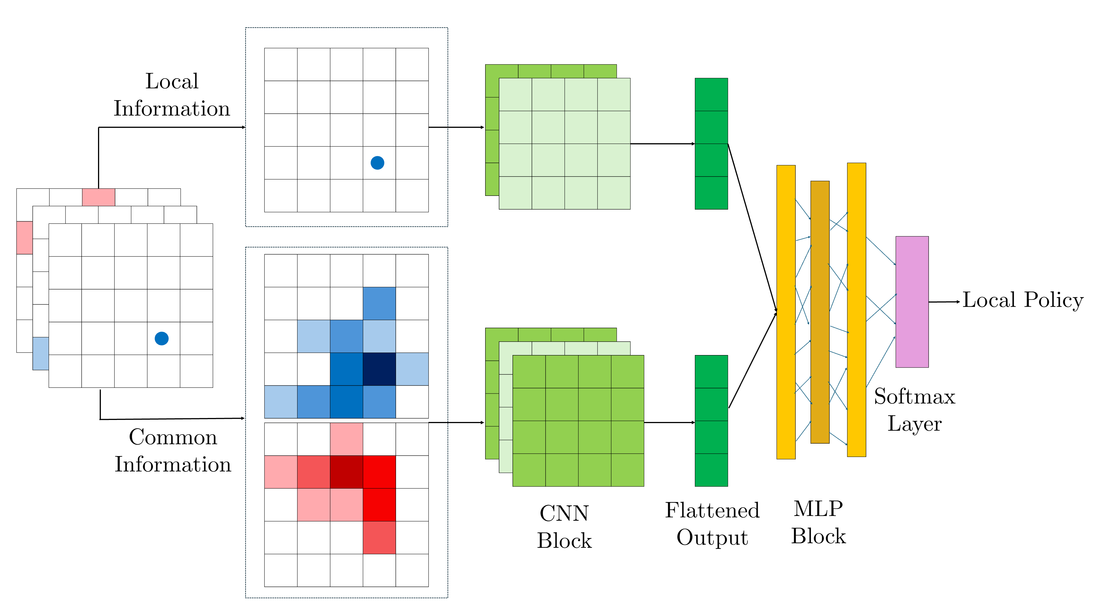
Figure C.1. MF-MAPPO: Shared-team actor for battlefield

The common information and local information are separated and passed through CNN blocks, the outputs of which are then flattened, combined and passed through an MLP block followed by a softmax layer which results in the action distribution for the given state.

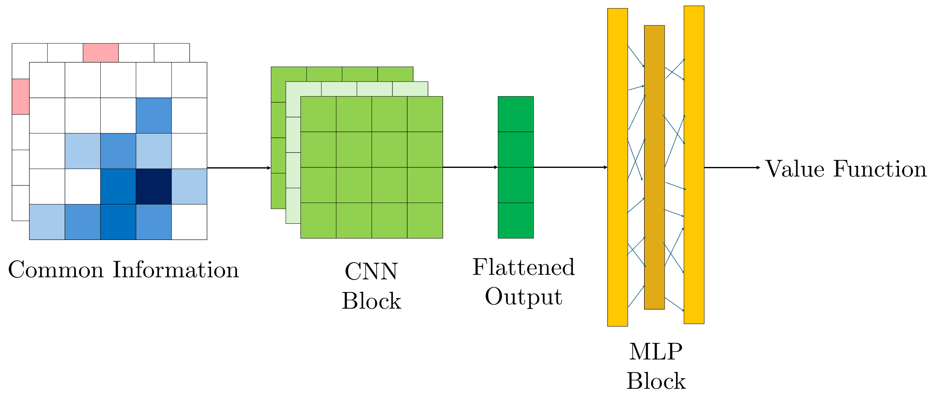
Figure C.2. MF-MAPPO: Minimally-informed critic for battlefield

The common information is passed through a CNN block which is then flattened and passed through an MLP block which outputs the value function.

All maps are trained using a single NVIDIA GeForce RTX 3070 GPU. The actor and critic learning rates are set to 0.0005 and 0.001 and both decay geometrically by a factor of 0.999. The networks are updated using the ADAM optimizer Kingma and Ba (2017) with two mini-batches for 10 epochs and a PPO clip value of 0.1. The entropy coefficient is initialized to 0.01 and decays with a factor of 0.995.

Maps 1 and 2 which are $4\times 4$ grid worlds are trained for $5\times 10^{6}$ and $4.5\times 10^{6}$ time steps, respectively, and in both cases, the episode length is 20 time steps and the update frequency is every 500 time steps. The total training period is about one day. On the other hand, Map 3 being $8\times 8$ in dimension, has an episode length of 64, is trained for $9\times 10^{6}$ time steps and its network is updated every 1,000 time steps. The total training period is approximately three days.

Appendix D Additional Results

In this section, we present additional simulation results from the zero-sum battlefield game.

D.1. Validation Cases for MF-MAPPO

The following subsection qualitatively discusses the battlefield game for different map layouts. For these results, both teams are deploying policies trained using MF-MAPPO.

Map A

The first map is a simple $4\times 4$ grid world with a single target that we use to validate our algorithm. The target is partially blocked by an obstacle, see Figure D.3. For the initial condition in Figure D.3, the Blue team is initially split into two equal groups. The Blue team decides to merge the two sub-groups of agents into a single group. With this formation, the Red team has zero numerical advantage over the Blue team when they encounter in (g), resulting in all Blue agents safely arriving at the target. In comparison, if the two Blue subgroups do not merge but move toward the target one at a time, it will lead to 50% of the Blue team population being deactivated (first subgroup), followed by the remaining 50% (second subgroup). This demonstrates how the observation of mean-field distributions guides rational decision-making.

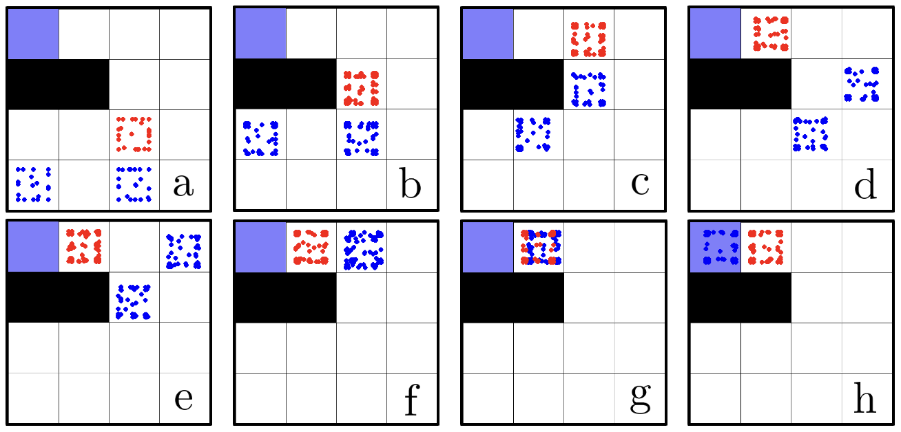
Figure D.3. Red is concentrated; Blue is evenly split.

MF-MAPPO Performance for Two Team Offense-Defense where Blue agents are attacking and Red are defending: Red team is concentrated while the Blue team is evenly split between the two cells.

Map B

This map is identical to the one presented in Section 5.3. In the first scenario (Figure D.4), 70% of the Blue agents start at cell [2, 2], and 30% at cell [1, 1], while the Red team is evenly split between cells [0, 1] and [3, 3]. Half of the Red team at [0, 1] successfully blocks the 30% Blue agent group from entering the left corridor due to its numerical advantage, which forces the Blue agents to opt for the right corridor. At the same time, the larger Blue group with 70% of the population utilized their numerical advantage over the half Red team at the top right and deactivated all the Red agents as shown in (c) and reached the target at time step (d). This allowed the smaller 30% group to follow through the same corridor without losing agents.

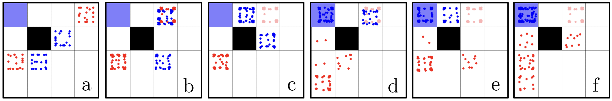
Figure D.4. Red is evenly split; 30% Blue are at $[1,1]$ and 70% are at $[2,2]$.

MF-MAPPO Performance for Two Team Offense-Defense where Blue agents are attacking and Red are Defending: Red is evenly split while 30% are at $[1,1]$ and 70% are at $[2,2]$.

In the second scenario (Figure D.5), with the Red team evenly distributed at the corners, 30% of the Blue agents start at cell [2, 2] and 70% at cell [3, 1]. The Red team’s numerical advantage at [3, 3] forces the Blue agents to move around and regroup (Figures D.5(b)-D.5(f)). Once united, the Blue team’s numerical advantage forces the Red subgroup at [0,1] to disperse to avoid deactivation, allowing Blue to reach the target.

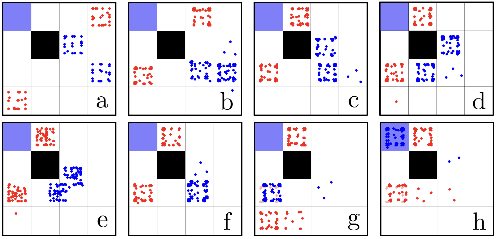
Figure D.5. Red is evenly split; 70% Blue are at $[3,1]$ and 30% are at $[2,2]$.

MF-MAPPO Performance for Two Team Offense-Defense where Blue agents are attacking and Red are Defending: Red is evenly split while 70% are at $[3,1]$ and 30% are at $[2,2]$.

Map C

Subsection 5.3 presented scenarios featuring structured initial configurations for both teams over an $8\times 8$ grid. It is important to emphasize, however, that the algorithm is trained on a diverse set of initial conditions for a given map, ranging from agents concentrated within a few selected cells to agents distributed randomly across the grid world. The following examples demonstrate that the teams are able to accomplish their objectives even in scenarios where agents are dispersed across the environment rather than clustered into just 1-2 subgroups.

In Figure D.6, the Blue team is initialized randomly, and local subgroups of agents emerge and coordinate to reach the target. This behavior is particularly pronounced near the upper target, where a greater numerical advantage facilitates successful coalition formation (Figures D.6(c)–(e)).

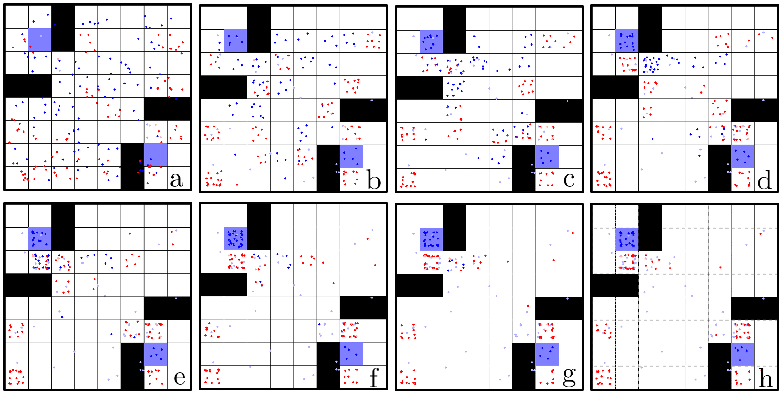
Figure D.6. Blue team is randomly spread around the map.

Blue team is randomly spread around the map.

Turning to the randomly distributed Red team agents in Figure D.7, it is observed that they concentrate near the two target entrances and successfully neutralize most Blue team subgroups.

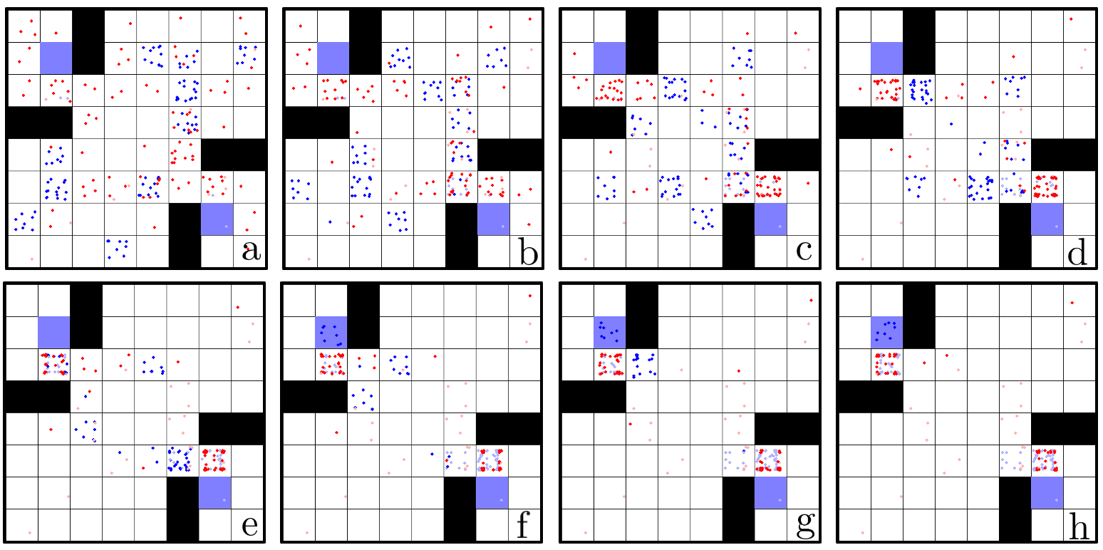
Figure D.7. Red team is randomly spread around the map.

Red team is randomly spread around the map.

D.2. Comparison with Baseline

Initial Condition 1

We focus on the same initial conditions as in Figure 9, but now pit the Blue team against the MF-MAPPO defenders instead of the DDPG-MFTG defenders (Figures 9(c) and D.8). The results align with those in Figure 8, where MF-MAPPO Blue agents effectively leverage their numerical advantage, enabling a larger number of agents to reach the target.

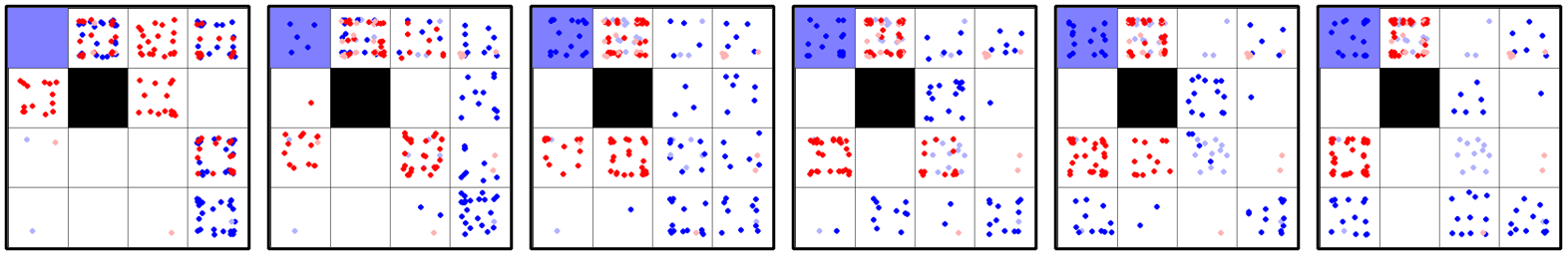
Figure D.8. MF-MAPPO Red vs. DDPG-MFTG Blue.

DDPG-MFTG Blue vs. MF-MAPPO Red.

Initial Condition 2

In Figures D.9 and 10(c), the defenders deactivate the Blue agents under both algorithms. However, similar to the results in Figure 10, MF-MAPPO agents actively learn to block the targets.

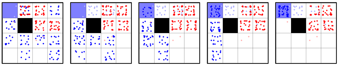
Figure D.9. MF-MAPPO Blue vs. DDPG-MFTG Red.

MF-MAPPO Blue vs. DDPG-MFTG Red.

Initial Condition 3

We present a final initial condition for the $4\times 4$ Battlefield game (Figure D.10, where, using similar arguments as in the previous two cases, we can establish the superiority of MF-MAPPO agents over the baseline DDPG-MFTG, whether MF-MAPPO serves as the attacker or the defender.

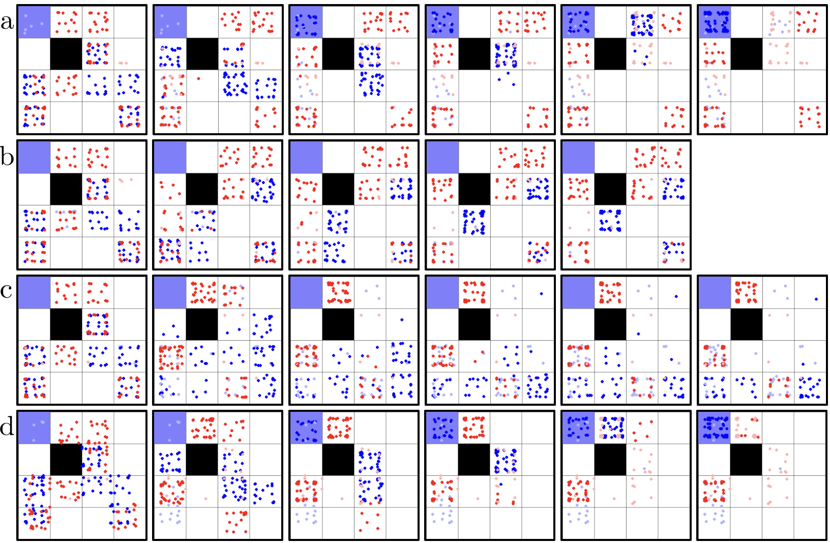
Figure D.10. a. MF-MAPPO Blue vs. DDPG-MFTG Red; b. DDPG-MFTG Blue vs. DDPG-MFTG Red; c. MF-MAPPO Red vs. DDPG-MFTG Blue; d. MF-MAPPO Red vs. MF-MAPPO Blue.

a. MF-MAPPO Blue vs. DDPG-MFTG Red; b. DDPG-MFTG Blue vs. DDPG-MFTG Red; c. MF-MAPPO Red vs. DDPG-MFTG Blue; d. MF-MAPPO Red vs. MF-MAPPO Blue

References

- (1)
- Arabneydi and Mahajan (2015) Jalal Arabneydi and Aditya Mahajan. 2015. Team-optimal solution of finite number of mean-field coupled LQG subsystems. In 54th IEEE Conference on Decision and Control. IEEE, Osaka, Japan, Dec. 15–18, 2015, 5308–5313.
- Cui et al. (2024) Kai Cui, Sascha Hauck, Christian Fabian, and Heinz Koeppl. 2024. Learning Decentralized Partially Observable Mean Field Control for Artificial Collective Behavior. arXiv:2307.06175 [cs.LG] https://arxiv.org/abs/2307.06175
- Cui and Koeppl (2022) Kai Cui and Heinz Koeppl. 2022. Approximately Solving Mean Field Games via Entropy-Regularized Deep Reinforcement Learning. arXiv:2102.01585 [cs.MA] https://arxiv.org/abs/2102.01585
- Guan et al. (2024) Yue Guan, Mohammad Afshari, and Panagiotis Tsiotras. 2024. Zero-Sum Games between Mean-Field Teams: Reachability-Based Analysis under Mean-Field Sharing. Proceedings of the AAAI Conference on Artificial Intelligence 38, 9 (Mar. 2024), 9731–9739. https://doi.org/10.1609/aaai.v38i9.28831
- Guan et al. (2022) Yue Guan, Mi Zhou, Ali Pakniyat, and Panagiotis Tsiotras. 2022. Shaping large population agent behaviors through entropy-regularized mean-field games. In 2022 American Control Conference (ACC). IEEE, IEEE, Atlanta, USA, June 08–10, 2022, 4429–4435.
- Huang et al. (2006) Minyi Huang, Roland P. Malhamé, and Peter E. Caines. 2006. Large population stochastic dynamic games: closed-loop McKean-Vlasov systems and the Nash certainty equivalence principle. Communications in Information & Systems 6, 3 (2006), 221 – 252.
- Huang et al. (2022) Shengyi Huang, Rousslan Fernand Julien Dossa, Antonin Raffin, Anssi Kanervisto, and Weixun Wang. 2022. The 37 Implementation Details of Proximal Policy Optimization. https://iclr-blog-track.github.io/2022/03/25/ppo-implementation-details/ https://iclr-blog-track.github.io/2022/03/25/ppo-implementation-details/.
- Kingma and Ba (2017) Diederik P. Kingma and Jimmy Ba. 2017. Adam: A Method for Stochastic Optimization. arXiv:1412.6980 [cs.LG] https://arxiv.org/abs/1412.6980
- Lanctot et al. (2017) Marc Lanctot, Vinicius Zambaldi, Audrūnas Gruslys, Angeliki Lazaridou, Karl Tuyls, Julien Pérolat, David Silver, and Thore Graepel. 2017. A unified game-theoretic approach to multiagent reinforcement learning. In Proceedings of the 31st International Conference on Neural Information Processing Systems (Long Beach, California, USA) (NIPS’17). Curran Associates Inc., Red Hook, NY, USA, 4193–4206.
- Lillicrap et al. (2019) Timothy P. Lillicrap, Jonathan J. Hunt, Alexander Pritzel, Nicolas Heess, Tom Erez, Yuval Tassa, David Silver, and Daan Wierstra. 2019. Continuous control with deep reinforcement learning. arXiv:1509.02971 [cs.LG] https://arxiv.org/abs/1509.02971
- Lowe et al. (2017) Ryan Lowe, Yi Wu, Aviv Tamar, Jean Harb, Pieter Abbeel, and Igor Mordatch. 2017. Multi-agent actor-critic for mixed cooperative-competitive environments. In Proceedings of the 31st International Conference on Neural Information Processing Systems (Long Beach, California, USA) (NIPS’17). Curran Associates Inc., Red Hook, NY, USA, 6382–6393.
- Nayyar et al. (2013) Ashutosh Nayyar, Aditya Mahajan, and Demosthenis Teneketzis. 2013. Decentralized stochastic control with partial history sharing: A common information approach. IEEE Trans. Automat. Control 58, 7 (2013), 1644–1658.
- Osborne (2004) Martin J Osborne. 2004. An Introduction to Game Theory. Oxford University Press 2 (2004), 672–713.
- Raghavan (1994) TES Raghavan. 1994. Zero-sum two-person games. Handbook of game theory with economic applications 2 (1994), 735–768.
- Saldi et al. (2023) Naci Saldi, Tamer Başar, and Maxim Raginsky. 2023. Partially observed discrete-time risk-sensitive mean field games. Dynamic Games and Applications 13, 3 (2023), 929–960.
- Schulman et al. (2018) John Schulman, Philipp Moritz, Sergey Levine, Michael Jordan, and Pieter Abbeel. 2018. High-Dimensional Continuous Control Using Generalized Advantage Estimation. arXiv:1506.02438 [cs.LG] https://arxiv.org/abs/1506.02438
- Schulman et al. (2017) John Schulman, Filip Wolski, Prafulla Dhariwal, Alec Radford, and Oleg Klimov. 2017. Proximal Policy Optimization Algorithms. arXiv:1707.06347 [cs.LG] https://arxiv.org/abs/1707.06347
- Sen and Caines (2019) Nevroz Sen and Peter E Caines. 2019. Mean field games with partial observation. SIAM Journal on Control and Optimization 57, 3 (2019), 2064–2091.
- Shao et al. (2024) Kai Shao, Jiacheng Shen, Chijie An, and Mathieu Laurière. 2024. Reinforcement Learning for Finite Space Mean-Field Type Games. arXiv:2409.18152 [cs.GT] https://arxiv.org/abs/2409.18152
- Smith et al. (2021) Max Olan Smith, Thomas Anthony, and Michael P. Wellman. 2021. Iterative Empirical Game Solving via Single Policy Best Response. arXiv:2106.01901 [cs.MA] https://arxiv.org/abs/2106.01901
- Sorin (2002) Sylvain Sorin. 2002. A First Course on Zero-Sum Repeated Games. Vol. 37. Springer Science & Business Media, Berlin.
- Tamar et al. (2016) Aviv Tamar, Dotan Di Castro, and Shie Mannor. 2016. Learning the variance of the reward-to-go. Journal of Machine Learning Research 17, 13 (2016), 1–36.
- Wang et al. (2022) Guofang Wang, Ziming Li, Wang Yao, and Sikai Xia. 2022. A multi-population mean-field game approach for large-scale agents cooperative attack-defense evolution in high-dimensional environments. Mathematics 10, 21 (2022), 4075.
- Yang et al. (2020) Yaodong Yang, Rui Luo, Minne Li, Ming Zhou, Weinan Zhang, and Jun Wang. 2020. Mean Field Multi-Agent Reinforcement Learning. arXiv:1802.05438 [cs.MA] https://arxiv.org/abs/1802.05438
- Yardim and He (2024) Batuhan Yardim and Niao He. 2024. Exploiting Approximate Symmetry for Efficient Multi-Agent Reinforcement Learning. arXiv:2408.15173 [cs.GT] https://arxiv.org/abs/2408.15173
- Yu et al. (2022) Chao Yu, Akash Velu, Eugene Vinitsky, Jiaxuan Gao, Yu Wang, Alexandre Bayen, and Yi Wu. 2022. The surprising effectiveness of ppo in cooperative multi-agent games. Advances in Neural Information Processing Systems 35 (2022), 24611–24624.