Refined Predictions for Starobinsky Inflation and Post-inflationary Constraints
in Light of ACT

Abstract

Recent measurements from the Atacama Cosmology Telescope (ACT), combined with Planck and DESI data, suggest a higher value for the spectral index $n_{s}$. This places Starobinsky inflation at the edge of the $2\sigma$ constraints for a number of e-folds $N_{\star}$ around $60$ when using the usual analytical approximations. We present refined predictions for Starobinsky inflation that go beyond the commonly used analytical approximations. By evaluating the model with these improved expressions, we show that for $N_{\star}\gtrsim 60$ it remains consistent with current observational constraints at the $2\sigma$ level. Additionally, we examine the implications of the ACT results for post-inflationary reheating parameters. Specifically, we find a lower bound on the effective equation of state parameter during reheating of approximately $\omega\gtrsim 0.462$; this excludes purely perturbative reheating, which leads to $\omega\simeq 0$. We also show that the reheating temperature is constrained to be $T_{\text{rh}}\lesssim 2\times 10^{12}~\text{GeV}$, assuming $\omega\leq 1$. Furthermore, we find that the predictions for the spectral index and tensor-to-scalar ratio can lie within $1\sigma$ of the recent ACT constraints if the reheating temperature satisfies $4~\text{MeV}\lesssim T_{\text{rh}}\lesssim 10~\text{GeV}$ for $0.8\lesssim\omega\leq 1$.

MITP-25-033

1 Introduction

Cosmic inflation offers an elegant solution to several key problems in cosmology Starobinsky:1980te ; Guth:1980zm ; Linde:1981mu ; Albrecht:1982wi , with detailed reviews available in Refs. Olive:1989nu ; Martin:2013tda ; Ellis:2023wic . It predicts a nearly scale-invariant power spectrum, which is typically characterized by the spectral index $n_{s}$. The Planck 2018 results report a value of $n_{s}=0.965\pm 0.004$ Planck:2018vyg ; Planck:2018jri . More recent data from the Atacama Cosmology Telescope (ACT) suggest a higher value for $n_{s}$ ACT:2025fju ; ACT:2025tim . Specifically, Ref. ACT:2025fju shows that combining Planck, ACT, and DESI data DESI:2024uvr ; DESI:2024mwx yields $n_{s}=0.974\pm 0.003$. Additionally, Ref. ACT:2025tim finds that Starobinsky inflation Starobinsky:1980te is located at the $2\sigma$ boundary of the combined constraints, with the number of e-folds before the end of inflation estimated at around $60$. These results have sparked several discussions and (or) alternative proposals in response to the ACT results  Kallosh:2025rni ; Aoki:2025wld ; Berera:2025vsu ; Dioguardi:2025vci ; Salvio:2025izr ; Dioguardi:2025mpp ; Rehman:2025fja ; Gao:2025onc ; He:2025bli ; Gialamas:2025kef .

In this work, we revisit the predictions within the Starobinsky inflationary framework. We begin by recalling that, in the limit of large $N_{\star}$ (the number of e-folds before the end of inflation), the inflationary predictions of the Starobinsky model can be approximated as Ellis:2013nxa ; Kallosh:2013maa ; Kallosh:2013yoa ; Motohashi:2014tra

$$n_{s} \simeq 1-\frac{2}{N_{\star}},\quad r\simeq\frac{12}{N_{\star}^{2}}\,,$$ (1)

where $n_{s}$ is the spectral index and $r$ is the tensor-to-scalar ratio.

Given the recent advances in the measurement of $n_{s}$, it has become essential to employ more accurate theoretical predictions when confronting observational results. Motivated by this, one of the main objectives of this work is to provide simple yet more precise expressions for the inflationary observables, particularly for $n_{s}$, within the Starobinsky model. Additionally, we aim to investigate the resulting constraints on reheating parameters derived from the recent combined measurements of $n_{s}$; this is another goal of this work.

The rest of this article is organized as follows. In Section 2, we revisit Starobinsky inflation, focusing on the derivation of more precise expressions for its inflationary predictions. In Section 3, we compare these results with the commonly used approximations and confront them with the recent ACT results. We then investigate the implications for post-inflationary reheating parameters in Section 4. Finally, we summarize the main findings of this work in Section 5.

2 Starobinsky Inflation and Predictions

In this section, we briefly revisit Starobinsky inflation Starobinsky:1980te , one of the earliest predictive models of inflation. The theory is based on a modification of general relativity, and is described by the action

$$S\supset\frac{M_{\rm Pl}^{2}}{2}\int d^{4}x\sqrt{-g}\left(R+\frac{1}{6M^{2}}R^{2}\right),$$ (2)

where $g$ is the determinant of the metric $g_{\mu\nu}$, $R$ is the Ricci scalar, $M_{\rm Pl}$ denotes the reduced Planck mass, and $M$ is a mass scale associated with the inflationary dynamics. The presence of the $R^{2}$ term leads to a period of accelerated expansion in the early Universe, without invoking an explicit scalar inflaton field.

By performing a conformal transformation to the Einstein frame, the theory can be recast as a scalar field theory with a canonical kinetic term and an effective potential given by Ellis:2013nxa ; Kallosh:2013yoa ; Motohashi:2014tra ; Ellis:2021kad

$$V(\phi)=\frac{3M^{2}M_{\rm Pl}^{2}}{4}\left(1-e^{-\sqrt{\frac{2}{3}}\frac{\phi}{M_{\rm Pl}}}\right)^{2}.$$ (3)

This potential features a plateau at large inflaton field values, supporting slow-roll (SR) inflation.

To obtain the inflationary predictions, we apply the SR formalism and define the following SR parameters

$$\epsilon_{V}\equiv\frac{M_{\rm Pl}^{2}}{2}\left(\frac{V^{\prime}}{V}\right)^{2},\quad\eta_{V}\equiv M_{\rm Pl}^{2}\,\frac{V^{\prime\prime}}{V}\,,$$ (4)

whose magnitude must be smaller than one during the accelerated expansion of the Universe. Here, $\prime$ means the derivative of the potential with respect to $\phi$. Inflation ends when the field reaches the value $\phi=\phi_{\text{end}}$ defined as $\epsilon_{V}(\phi_{\text{end}})=1$ in the current large field setup. The total number of e-folds $N_{\star}$ between the time when the Cosmic Microwave Background (CMB) pivot scale $k_{\star}=0.05$ Mpc^-1 first crossed the horizon (with a field value $\phi=\phi_{\star}$) until the end of inflation is given by

$$N_{\star} =\int^{\phi_{\star}}_{\phi_{\text{end}}}\frac{1}{\sqrt{2\,\epsilon_{V}(\phi)}}\,\frac{d\phi}{M_{\rm Pl}}\,.$$ (5)

The power spectrum of the curvature perturbation $A_{s}$, the spectral index $n_{s}$, and the tensor-to-scalar ratio $r$ are respectively given by

$$A_{s} =\frac{1}{24\pi^{2}\,\epsilon_{V}}\,\frac{V}{M_{\rm Pl}^{4}}\,,$$ (6)

$$n_{s} =1-6\epsilon_{V}+2\eta_{V}\,,$$ (7)

$$r =16\epsilon_{V}\,,$$ (8)

in the SR formalism. The central value of the power spectrum is $A_{s}=2.1\times 10^{-9}$ Planck:2018vyg , which allows one to determine the scale of $M$. We note that the inflationary predictions $n_{s}$ and $r$ are independent of $M$, as will be shown below.

Using the potential in Eq. (3), we find the tensor-to-scalar ratio and spectral index can be written as

$$r =\frac{64}{3\left(e^{\sqrt{\frac{2}{3}}\frac{\phi_{\star}}{M_{\rm Pl}}}-1\right)^{2}}\,,$$ (9)

$$n_{s} =\frac{3\left(e^{\sqrt{\frac{2}{3}}\frac{\phi_{\star}}{M_{\rm Pl}}}-1\right)^{2}-8\left(e^{\sqrt{\frac{2}{3}}\frac{\phi_{\star}}{M_{\rm Pl}}}+1\right)}{3\left(e^{\sqrt{\frac{2}{3}}\frac{\phi_{\star}}{M_{\rm Pl}}}-1\right)^{2}}\,.$$ (10)

Note that in the large-field limit, where the potential becomes flat, one finds the expected behavior: $r\to 0$ and $n_{s}\to 1$.

The field value at the end of inflation is given by

$$\phi_{\text{end}}=M_{\rm Pl}\sqrt{\frac{3}{2}}\ln\left(1+\frac{2}{\sqrt{3}}\right)\,.$$ (11)

From Eq. (10), one can solve for $\phi_{\star}$ with a given $n_{s}$:

$$\phi_{\star}=M_{\rm Pl}\sqrt{\frac{3}{2}}\ln\left[\frac{7+4\sqrt{4-3\,n_{s}}-3\,n_{s}}{3(1-n_{s})}\right]\,,$$ (12)

which, with Eq. (9), yields

$$r =\frac{4}{3}\left[3(1-n_{s})+2-2\sqrt{3(1-n_{s})+1}\right]\,.$$ (13)

We note that Eq.(13) has been presented earlier in Ref. Garcia:2023tkk .

The total number e-folds $N_{\star}$ in Eq. (5) can also expressed as a function of $n_{s}$:

$$N_{\star} =\int^{\phi_{\star}}_{\phi_{\text{end}}}\frac{1}{\sqrt{2\epsilon_{V}}}\frac{d\phi}{M_{\rm Pl}}=\frac{3}{4}\left[e^{\sqrt{\frac{2}{3}}\frac{\phi_{\star}}{M_{\rm Pl}}}-e^{\sqrt{\frac{2}{3}}\frac{\phi_{\text{end}}}{M_{\rm Pl}}}-\sqrt{\frac{2}{3}}\frac{\left(\phi_{\star}-\phi_{\text{end}}\right)}{M_{\rm Pl}}\right]\,$$

$$=\frac{2-\sqrt{3}(1-n_{s})+2\sqrt{3(1-n_{s})+1}}{2(1-n_{s})}-\frac{3}{4}\ln\left[\frac{4+3(1-n_{s})+4\sqrt{3(1-n_{s})+1}}{(1-n_{s})(2\sqrt{3}+3)}\right]\,$$

$$=\frac{2-\sqrt{3}t+2\sqrt{3t+1}}{2t}-\frac{3}{4}\ln\left[\frac{4+3t+4\sqrt{3t+1}}{t(2\sqrt{3}+3)}\right]\,,$$ (14)

where we have introduced a small parameter $t\equiv 1-n_{s}$ in the last step.

We now discuss how the exact results obtained above reduce to the commonly used approximations shown in Eq. (1). Noting that $n_{s}$ is close to unity, we write the last line of Eq. (2) as

$$N_{\star} \simeq\frac{2}{t}+\frac{1}{4}\left[6-2\sqrt{3}+3\ln\left(\frac{3+2\sqrt{3}}{8}\right)+3\ln t\right]+\mathcal{O}(t)\,$$

$$\simeq\frac{2}{1-n_{s}}+\frac{3}{4}\ln(1-n_{s})+0.47+\mathcal{O}(1-n_{s})\,.$$ (15)

Note that the second term in Eq. (2) is negative and of order unity, which effectively reduces the value of $N_{\star}$ for given $n_{s}$. Similarly, the tensor-to-scalar ratio given in Eq. (13) can be expanded as

$$r \simeq 3t^{2}+\frac{9}{2}t^{3}+\mathcal{O}(t^{4})\,$$

$$\simeq 3(1-n_{s})^{2}+\frac{9}{2}(1-n_{s})^{3}+\mathcal{O}[(1-n_{s})^{4}]\,.$$ (16)

It is interesting to observe that Eq. (2) can be solved iteratively to obtain a simple yet precise relation between $n_{s}$ and $N_{\star}$; combined with the first term in Eq. (2), this yields

$$n_{s}\simeq 1-\frac{2}{N_{\star}-\frac{3}{4}\ln\left(\frac{2}{N_{\star}}\right)}\,,\quad r\simeq\frac{12}{\left[N_{\star}-\frac{3}{4}\ln\left(\frac{2}{N_{\star}}\right)\right]^{2}}\,,$$ (17)

which match very well with the exact results shown in Eq. (13) and Eq. (2). To the best of our knowledge, the expression for $n_{s}$ presented in Eq. (17) has not previously shown in the literature. We consider it to be one of the main result in this work, and we advocate its use when confronting the Starobinsky model with experimental data.

We now discuss how to reproduce the usual approximation Eq. (1) using Eq. (17). By retaining only the first terms both in Eq. (2) and Eq. (2) or dropping the term $-\frac{3}{4}\ln\left(\frac{2}{N_{\star}}\right)$ in Eq. (17), we recover the commonly used approximate expressions in Eq. (1):

$$n_{s}\simeq 1-\frac{2}{N_{\star}},\quad r\simeq\frac{12}{N_{\star}^{2}}\,.$$ (18)

Eq. (18) implies a relation

$$r\simeq 3(1-n_{s})^{2}\,,$$ (19)

which corresponds to the first term of Eq. (2). Since there is no term $\propto\ln(1-n_{s})$ in Eq. (2), Eq. (19) also holds for our refined approximation Eq. (17), up to corrections of relative order $1-n_{s}$

Before closing this section, we note that the spectral index $n_{s}$ in the approximation Eq. (18) is underestimated for a given number of e-folds $N_{\star}$, as is evident when compared with Eq. (17). These comparisons will be made more explicit in the next section, where we also discuss the implications with current experimental constraints.

3 Comparison between Exact and Approximate Results

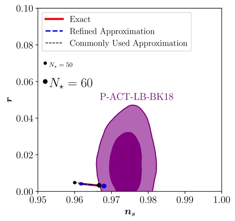
Figure 1: Comparison of the exact expression in Eq. (13) with the refined approximation in Eq. (17) and the commonly used approximation in Eq. (18) for $r$ and $n_{s}$ within the framework of Starobinsky inflation.

In this section, we compare the approximations in Eqs. (18) with the exact result given in Eq. (13), as well as with the refined approximation in Eq. (17), and confront them with current observational data.

The results are presented in Fig. 1, where we show the predictions in the $r$–$n_{s}$ plane, overlaid with the $2\sigma$ combined constraints from Planck, ACT, DESI, and BICEP/Keck data BICEP:2021xfz (P-ACT-LB-BK18), shown in purple and reproduced from Fig. 10 of Ref. ACT:2025tim . The red solid line shows the exact result based on Eq. (13), where $n_{s}$ is determined by Eq. (2) for a given number of e-folds. The blue dashed line depicts the refined approximation using Eq. (17). The black dashed line corresponds to the approximate relation obtained using Eqs. (18) and (19). The small and big dots denote $N_{\star}=50$ and $N_{\star}=60$, respectively.

As illustrated, the commonly used approximation in Eq. (18) (black dashed) suggests that Starobinsky inflation with $N_{\star}\leq 60$ lies near the boundary of the $2\sigma$ allowed region. In contrast, we show that the exact prediction (red solid), based on Eq. (13), remains within the $2\sigma$ allowed region at $N_{\star}=60$. It is also evident that the approximation in Eq. (18) underestimates the spectral index $n_{s}$. Furthermore, we demonstrate that the refined approximation Eq. (17) (blue dashed) provides a better fit to the exact prediction for $n_{s}$. These comparisons underscore the importance of employing more accurate theoretical expressions when interpreting current and future cosmological data.

Before closing this section, we note that we have so far considered $N_{\star}\in[50,60]$, which is typically a good assumption Liddle:2003as ; Dodelson:2003vq . However, $N_{\star}$ can also be larger, depending on the specifics of the post-inflationary expansion history Liddle:2003as ; Tanin:2020qjw . As we will demonstrate in the next section, a larger $N_{\star}$ can arise when matching with a post-inflationary phase that has a stiff background. As can be seen in Fig. 1, the prediction for $n_{s}$ can lie well within the $2\sigma$ region (even $1\sigma$ ) if $N_{\star}$ is sufficiently large. This underscores the necessity of consistently matching inflationary predictions with the subsequent expansion history, a topic we will discuss in the next section.

4 Constraints on Reheating

In this section, we investigate the implications of the ACT results for post-inflationary reheating parameters. Inflation must eventually come to an end, allowing the transfer of energy from the inflaton field to other particles, whose subsequent interactions lead to the formation of a thermal bath of Standard Model (SM) particles. The detailed dynamics of reheating, however, remain unknown and can be highly complex; see Refs. Allahverdi:2010xz ; Amin:2014eta ; Lozanov:2019jxc for reviews.

To facilitate reheating, the current setup shall be extended to allow the inflaton to decay or annihilate. Here, we remain agnostic about the specifics of reheating, and we parameterize the process using a few key quantities: the duration of reheating, defined as $N_{\text{rh}}\equiv\ln\left(a_{\text{rh}}/a_{\text{end}}\right)$, where $a_{\text{end}}$ and $a_{\text{rh}}$ are the scale factors at the end of inflation and at the end of reheating, respectively; the effective equation-of-state (EoS) parameter during reheating, $\omega$, such that the total energy density evolves as $\rho\propto a^{-3(1+\omega)}$; and the reheating temperature, $T_{\text{rh}}$, defined as the temperature of the thermal bath at the end of reheating. We define the end of reheating via $\rho(a_{\text{end}})=2\rho_{R}(a_{\text{end}})$, where $\rho_{R}=g_{\star}\pi^{2}T^{4}/30$ denotes the radiation energy density of the thermal bath with a temperature $T$. Here, $g_{\star}$ corresponds to the effective degrees of freedom contributing to the energy density in radiation $\rho_{R}$.

Depending on these parameters, the expansion history during reheating can vary, altering the time at which the CMB pivot scale reenters the horizon. This allows one to establish a relationship between the inflationary dynamics and the reheating parameters Dai:2014jja ; Cook:2015vqa ; Drewes:2017fmn . In particular, we have Cook:2015vqa ; Becker:2023tvd :

$$T_{\text{rh}}=\left[\left(\frac{43}{11\,g_{*s}(T_{\text{rh}})}\right)^{\frac{1}{3}}\frac{a_{0}T_{0}}{k_{\star}}H_{\star}e^{-N_{\star}}\left(\frac{45V_{\text{end}}}{\pi^{2}g_{*}(T_{\text{rh}})}\right)^{-\frac{1}{3\left(1+\omega\right)}}\right]^{\frac{3\left(1+\omega\right)}{3\omega-1}}\,,$$ (20)

for $\omega\neq 1/3$. Here, $a_{0}$ and $T_{0}=2.73~\text{K}$ correspond to the scale factor and temperature at present, respectively; $k_{\star}$ is the CMB pivot scale as mentioned in Section 2; $H_{\star}$ denotes the Hubble parameter when $\phi=\phi_{\star}$, given by $H_{\star}=\pi M_{\rm Pl}\sqrt{r(\phi_{\star})A_{s}(\phi_{\star})/2}$; $g_{\star s}$ is the effective degrees of freedom contributing to the total entropy densities; and $V_{\text{end}}$ is the potential energy at the end of inflation, i.e., when $\phi=\phi_{\text{end}}$ (cf. Eq. (11)).

Several remarks are in order regarding Eq.(20). We first note that the quantities with a $\star$ as subscript are defined as referring to the incident when the perturbation $k_{\star}$ crossed out of the Hubble horizon during inflation, i.e. $k_{\star}=a_{\star}H_{\star}$; hence $a_{0}H_{\star}/k_{\star}=a_{0}/a_{\star}$. For convenience we set $a_{0}=1$, which does not change the ratio $a_{0}/a_{\star}$. Moreover, we assume that only known particles in the SM contribute to $g_{\star}$ and $g_{\star s}$, in which case the effective number of relativistic degrees of freedom remains approximately constant at $106.75$ for temperatures above the top quark mass. At lower temperatures, however, $g_{\star}$ and $g_{\star s}$ vary; for instance, both are around $10.75$ when the reheating temperature is near the MeV scale. In our analysis, we have incorporated the temperature dependence of $g_{\star}$ and $g_{\star s}$ Drees:2015exa . We remind the reader that the inflationary predictions impacts $T_{\text{rh}}$ via the dependence on $H_{\star}$ and $N_{\star}$. Finally, we note that for the case with $\omega=1/3$, the distinction between the reheating stage and the radiation-dominated phase becomes ambiguous, in which case a simple correlation between inflationary predictions and reheating parameters cannot be derived Cook:2015vqa . Indeed, for the special case with $\omega=1/3$, one obtains the relation $61.5\simeq N_{\star}+\ln\left(\frac{V^{1/4}_{\text{end}}}{H\star}\right)$, assuming $g_{\star}=g_{\star s}=106.75$. This relation is independent of the reheating parameters and predicts a value of $n_{s}$ for a given inflationary model. In particular, we find that it yields $n_{s}\simeq 0.965$ for the Starobinsky inflation model under consideration.

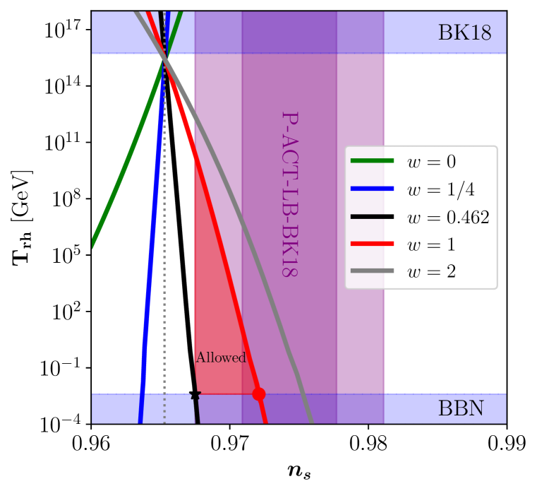
Figure 2: Reheating temperature $T_{\text{rh}}$ as a function of $n_{s}$ for different choices of the EoS parameter $\omega$ within the framework of Starobisnky inflation framework. The vertical dotted gray line corresponds to $\omega=1/3$.

In Fig. 2, we show the reheating temperature $T_{\text{rh}}$ as a function of $n_{s}$ and the EoS parameter $\omega$, together with the recent combined constraints on $n_{s}$ with ACT. The $1\sigma$ and $2\sigma$ region are indicated by the purple band. Additionally, we depict the constraints on the reheating temperature, including $T_{\text{rh}}\geq 4~\text{MeV}$ from Big Bang Nucleosynthesis (BBN) Kawasaki:2000en ; Hannestad:2004px ; DeBernardis:2008zz ; deSalas:2015glj and $T_{\text{rh}}\leq 5.5\times 10^{15}~\text{GeV}$ from the upper bound on the inflationary scale as measured by BICEP/KecK 2018 BICEP:2021xfz , shown in light blue.

$\omega$	$\text{Maximum}\,\,T_{\text{rh}}~[\text{GeV}]$
$0.462$	$4\times 10^{-3}$
$\frac{2}{3}$	$1\times 10^{7}$
$1$	$2\times 10^{10}$
$2$	$2\times 10^{12}$

Table 1: Maximum value $T_{\text{rh}}$ as a function of $\omega$ being consistent with the $2\sigma$ constraint on $n_{s}$ from the combined results from ACT.

The solid green, blue, black, red, and gray lines correspond to $\omega=0$, $\omega=1/4$, $\omega=0.462$, $\omega=1$, and $\omega=2$, respectively. We note that the reheating temperature, $T_{\text{rh}}$, decreases (increases) with $n_{s}$ for $\omega>1/3$ ($\omega<1/3$), as shown in Fig. 2. The special case $\omega=1/3$ corresponds to a vertical line at $n_{s}\simeq 0.965$, independent of $T_{\text{rh}}$, as indicated by the vertical gray line in Fig. 2. As $\omega$ approaches $1/3$, all curves are expected to converge toward the vertical gray line. A fixed point occurs at $T_{\text{rh}}\simeq 10^{15}\,\text{GeV}$ with $n_{s}\simeq 0.965$, where $d\,T_{\text{rh}}/d\,\omega\to 0$.

For $\omega=0$, we find that a reheating temperature $T_{\rm rh}\gtrsim 10^{20}$ GeV is required in order to be consistent with the $2\sigma$ value of $n_{s}$ from ACT; this is clearly unacceptable. $\omega=0$ is often associated with perturbative reheating, given that the potential (3) is quadratic near the origin, $V(\phi)\simeq M^{2}\phi^{2}/2+{\cal O}(\phi^{3})$. This also implies that the physical inflaton mass $m_{\phi}=M$. Since in a thermal bath the average particle energy $\langle E\rangle\sim 2.5T$, perturbative reheating via inflaton decay requires $T_{\rm rh}<m_{\phi}/5$, unless reactions that reduce the number of particles (e.g., $3\rightarrow 2$ reactions) are efficient, which seems highly implausible. For $\omega=0$ and $T_{\rm rh}<10^{13}$ GeV we find $n_{s}<0.964$, which is three standard deviations below the ACT result.

As $\omega$ increases, the curves shift from left to right, as seen in the green and blue curves. To satisfy the observational constraints, we find that $\omega\gtrsim 0.462$ is required. This is evident from the black solid line in Fig. 2, which touches the crossing point between the lower bound on $T_{\text{rh}}$ from BBN and the $2\sigma$ boundary from ACT. As $\omega$ increases further, the overlapping region expands from a point (the black star) into a finite area. The red line ($\omega=1$) crosses $T_{\text{rh}}=4~\text{MeV}$ at $n_{s}\simeq 0.972$, corresponding to $N_{\star}\simeq 69$; see also the red dot in Fig. 2. In this case, the allowed reheating parameter space for $\omega\leq 1$ is represented by the red-shaded region.

In Table 1, we show the maximum reheating temperature as a function of $\omega$. Assuming $\omega\leq 1$, the combined constraints for reheating parameters are found to be

$$0.462\lesssim\omega\,;\quad 4~\text{MeV}\leq T_{\text{rh}}\lesssim 2\times 10^{10}~\text{GeV}\,,$$ (21)

together with the inflationary parameters

$$0.967\lesssim n_{s}\lesssim 0.972\,;\quad 58\lesssim N_{\star}\lesssim 69\,,$$ (22)

in order to be consistent with the recent combined results on $n_{s}$ from ACT at $2\sigma$ level. Similarly, we can derive more stringent constraints at the $1\sigma$ level, finding that $0.804\lesssim\omega$ and $4~\text{MeV}\lesssim T_{\text{rh}}\lesssim 10~\text{GeV}$, with $0.971\lesssim n_{s}\lesssim 0.972$ and $66\lesssim N_{\star}\lesssim 69$. We note that for $\omega>1$, the upper bounds on $T_{\text{rh}}$ and $N_{\star}$ can be larger. For example, for $\omega=2$, the reheating temperature can reach $T_{\text{rh}}\simeq 10^{12}~\text{GeV}$ and $N_{\star}\simeq 78$ at the $2\sigma$ level of $n_{s}$. We note that a large EoS parameter, $\omega>0.5$, may be realized if the dynamics after the end of Starobinsky inflation transition to those driven by a potential significantly steeper than quadratic. For instance, if the inflaton oscillates around a potential of the form $\phi^{n}$, with $n$ being a positive even integer, the EoS parameter is given by $\omega=(n-2)/(n+2)$ Turner:1983he , implying that $\omega$ can approach unity for large $n$. Constructing a viable theory within the current framework that supports such large values of $\omega$ may nevertheless present challenges.

In Fig. 3, we depict the inflationary prediction (red solid line) consistent with the $2\sigma$ region of $n_{s}$ from ACT, considering $0.462\lesssim\omega\leq 1$. The corresponding predictions for the tensor-to-scalar ratio are

$$2\times 10^{-3}\lesssim r\lesssim 3\times 10^{-3}\,,$$ (23)

which can be tested by future precise cosmic microwave background (CMB) experiments. For instance, CORE COrE:2011bfs , AliCPT Li:2017drr , LiteBIRD Matsumura:2013aja , and CMB-S4 Abazajian:2019eic are expected to achieve sensitivity to $r\sim\mathcal{O}(10^{-3})$.

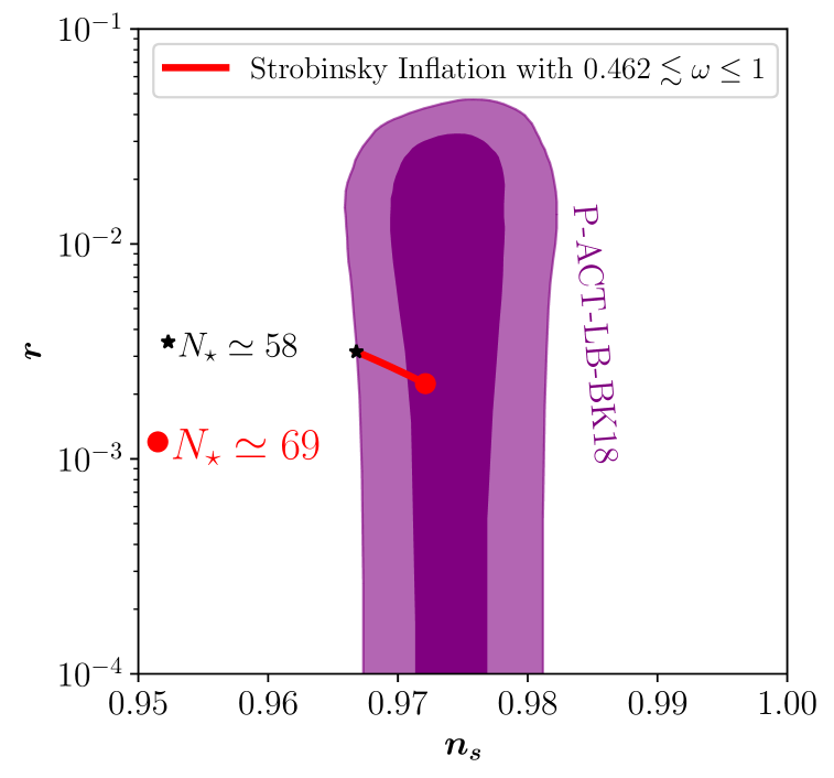
Figure 3: Inflationary predictions for the Starobinsky model with an effective post-inflationary EoS parameter $0.462\lesssim\omega\leq 1$ and $T_{\text{rh}}\geq 4~\text{MeV}$. The light purple region corresponds to the $2\sigma$ allowed region of $n_{s}$ from ACT.

5 Conclusion

In this work, we revisit the inflationary predictions of the Starobinsky model and investigate their compatibility with post-inflationary reheating dynamics, ensuring consistency with recent combined measurements of the spectral index from the Atacama Cosmology Telescope (ACT).

We present a refined approximation in Eq. (17), showing that when evaluated using these more accurate expressions, the predictions of the Starobinsky model remain consistent with the recent combined results from ACT at the $2\sigma$ level, as illustrated in Fig. 1. Relying on the commonly used approximations provided in Eq. (18) underestimates $n_{s}$, leading to an observation that the Starobinsky model with $N_{\star}\simeq 60$ lies at the edge of the $2\sigma$ constraints.

We also investigate the constraints on the reheating parameters. To this end, we parameterize reheating using an effective equation of state (EoS) parameter $\omega$, the reheating temperature $T_{\text{rh}}$, and the duration of reheating. The main results are presented in Fig. 2 and Table 1. Purely perturbative reheating, which leads to $\omega\simeq 0$ and $T_{\rm rh}\lesssim 10^{13}$ GeV, is disfavored at $\gtrsim 3\sigma$. We find that $\omega\gtrsim 0.462$ is needed in order to be consistent with Big Bang Nucleosynthesis (BBN) as well as the $2\sigma$ region of the combined ACT results for $n_{s}$. For $\omega\leq 1$, we derive an upper bound on the reheating temperature of approximately $T_{\text{rh}}\lesssim 2\times 10^{10}~\text{GeV}$. These results are summarized in Eq. (21). The combined inflationary predictions consistent with BBN as well as the $2\sigma$ region of $n_{s}$ from ACT results are depicted in Fig. 3 and can be tested by future cosmic microwave background (CMB) experiments.

In summary, we have provided refined approximations for the inflationary predictions of the Starobinsky model and derived constraints on the reheating parameters based on the latest combined experimental results on $n_{s}$ with ACT.

References

- (1) A.A. Starobinsky, A New Type of Isotropic Cosmological Models Without Singularity, Phys. Lett. B 91 (1980) 99.
- (2) A.H. Guth, The Inflationary Universe: A Possible Solution to the Horizon and Flatness Problems, Phys. Rev. D 23 (1981) 347.
- (3) A.D. Linde, A New Inflationary Universe Scenario: A Possible Solution of the Horizon, Flatness, Homogeneity, Isotropy and Primordial Monopole Problems, Phys. Lett. B 108 (1982) 389.
- (4) A. Albrecht and P.J. Steinhardt, Cosmology for Grand Unified Theories with Radiatively Induced Symmetry Breaking, Phys. Rev. Lett. 48 (1982) 1220.
- (5) K.A. Olive, Inflation, Phys. Rept. 190 (1990) 307.
- (6) J. Martin, C. Ringeval and V. Vennin, Encyclopædia Inflationaris: Opiparous Edition, Phys. Dark Univ. 5-6 (2014) 75 [1303.3787].
- (7) J. Ellis and D. Wands, Inflation (2023), 2312.13238.
- (8) Planck collaboration, Planck 2018 results. VI. Cosmological parameters, Astron. Astrophys. 641 (2020) A6 [1807.06209].
- (9) Planck collaboration, Planck 2018 results. X. Constraints on inflation, Astron. Astrophys. 641 (2020) A10 [1807.06211].
- (10) ACT collaboration, The Atacama Cosmology Telescope: DR6 Power Spectra, Likelihoods and CDM Parameters, 2503.14452.
- (11) ACT collaboration, The Atacama Cosmology Telescope: DR6 Constraints on Extended Cosmological Models, 2503.14454.
- (12) DESI collaboration, DESI 2024 III: baryon acoustic oscillations from galaxies and quasars, JCAP 04 (2025) 012 [2404.03000].
- (13) DESI collaboration, DESI 2024 VI: cosmological constraints from the measurements of baryon acoustic oscillations, JCAP 02 (2025) 021 [2404.03002].
- (14) R. Kallosh, A. Linde and D. Roest, A simple scenario for the last ACT, 2503.21030.
- (15) S. Aoki, H. Otsuka and R. Yanagita, Higgs-Modular Inflation, 2504.01622.
- (16) A. Berera, S. Brahma, Z. Qiu, R. O. Ramos and G.S. Rodrigues, The early universe is ACT-ing warm, 2504.02655.
- (17) C. Dioguardi, A.J. Iovino and A. Racioppi, Fractional attractors in light of the latest ACT observations, 2504.02809.
- (18) A. Salvio, Independent connection in ACTion during inflation, 2504.10488.
- (19) C. Dioguardi and A. Karam, Palatini Linear Attractors Are Back in ACTion, 2504.12937.
- (20) M.U. Rehman and Q. Shafi, Supersymmetric Hybrid Inflation in light of Atacama Cosmology Telescope Data Release 6, Planck 2018 and LB-BK18, 2504.14831.
- (21) Q. Gao, Y. Gong, Z. Yi and F. Zhang, Non-minimal coupling in light of ACT, 2504.15218.
- (22) M. He, M. Hong and K. Mukaida, Increase of in regularized pole inflation & Einstein-Cartan gravity, 2504.16069.
- (23) I.D. Gialamas, A. Karam, A. Racioppi and M. Raidal, Has ACT measured radiative corrections to the tree-level Higgs-like inflation?, 2504.06002.
- (24) J. Ellis, D.V. Nanopoulos and K.A. Olive, Starobinsky-like Inflationary Models as Avatars of No-Scale Supergravity, JCAP 10 (2013) 009 [1307.3537].
- (25) R. Kallosh and A. Linde, Non-minimal Inflationary Attractors, JCAP 10 (2013) 033 [1307.7938].
- (26) R. Kallosh, A. Linde and D. Roest, Superconformal Inflationary -Attractors, JHEP 11 (2013) 198 [1311.0472].
- (27) H. Motohashi, Consistency relation for inflation, Phys. Rev. D 91 (2015) 064016 [1411.2972].
- (28) J. Ellis, M.A.G. Garcia, D.V. Nanopoulos, K.A. Olive and S. Verner, BICEP/Keck constraints on attractor models of inflation and reheating, Phys. Rev. D 105 (2022) 043504 [2112.04466].
- (29) M.A.G. Garcia, G. Germán, R. Gonzalez Quaglia and A.M.M. Colorado, Reheating constraints and consistency relations of the Starobinsky model and some of its generalizations, JCAP 12 (2023) 015 [2306.15831].
- (30) BICEP, Keck collaboration, Improved Constraints on Primordial Gravitational Waves using Planck, WMAP, and BICEP/Keck Observations through the 2018 Observing Season, Phys. Rev. Lett. 127 (2021) 151301 [2110.00483].
- (31) A.R. Liddle and S.M. Leach, How long before the end of inflation were observable perturbations produced?, Phys. Rev. D 68 (2003) 103503 [astro-ph/0305263].
- (32) S. Dodelson and L. Hui, A Horizon Ratio Bound for Inflationary Fluctuations, Phys. Rev. Lett. 91 (2003) 131301 [astro-ph/0305113].
- (33) E.H. Tanin and T. Tenkanen, Gravitational wave constraints on the observable inflation, JCAP 01 (2021) 053 [2004.10702].
- (34) R. Allahverdi, R. Brandenberger, F.-Y. Cyr-Racine and A. Mazumdar, Reheating in Inflationary Cosmology: Theory and Applications, Ann. Rev. Nucl. Part. Sci. 60 (2010) 27 [1001.2600].
- (35) M.A. Amin, M.P. Hertzberg, D.I. Kaiser and J. Karouby, Nonperturbative Dynamics Of Reheating After Inflation: A Review, Int. J. Mod. Phys. D 24 (2014) 1530003 [1410.3808].
- (36) K.D. Lozanov, Lectures on Reheating after Inflation, 1907.04402.
- (37) L. Dai, M. Kamionkowski and J. Wang, Reheating constraints to inflationary models, Phys. Rev. Lett. 113 (2014) 041302 [1404.6704].
- (38) J.L. Cook, E. Dimastrogiovanni, D.A. Easson and L.M. Krauss, Reheating predictions in single field inflation, JCAP 04 (2015) 047 [1502.04673].
- (39) M. Drewes, J.U. Kang and U.R. Mun, CMB constraints on the inflaton couplings and reheating temperature in -attractor inflation, JHEP 11 (2017) 072 [1708.01197].
- (40) M. Becker, E. Copello, J. Harz, J. Lang and Y. Xu, Confronting dark matter freeze-in during reheating with constraints from inflation, JCAP 01 (2024) 053 [2306.17238].
- (41) M. Drees, F. Hajkarim and E.R. Schmitz, The Effects of QCD Equation of State on the Relic Density of WIMP Dark Matter, JCAP 06 (2015) 025 [1503.03513].
- (42) M. Kawasaki, K. Kohri and N. Sugiyama, MeV scale reheating temperature and thermalization of neutrino background, Phys. Rev. D 62 (2000) 023506 [astro-ph/0002127].
- (43) S. Hannestad, What is the lowest possible reheating temperature?, Phys. Rev. D 70 (2004) 043506 [astro-ph/0403291].
- (44) F. De Bernardis, L. Pagano and A. Melchiorri, New constraints on the reheating temperature of the universe after WMAP-5, Astropart. Phys. 30 (2008) 192.
- (45) P.F. de Salas, M. Lattanzi, G. Mangano, G. Miele, S. Pastor and O. Pisanti, Bounds on very low reheating scenarios after Planck, Phys. Rev. D 92 (2015) 123534 [1511.00672].
- (46) M.S. Turner, Coherent Scalar Field Oscillations in an Expanding Universe, Phys. Rev. D 28 (1983) 1243.
- (47) COrE collaboration, COrE (Cosmic Origins Explorer) A White Paper, 1102.2181.
- (48) H. Li et al., Probing Primordial Gravitational Waves: Ali CMB Polarization Telescope, Natl. Sci. Rev. 6 (2019) 145 [1710.03047].
- (49) T. Matsumura et al., Mission design of LiteBIRD, J. Low Temp. Phys. 176 (2014) 733 [1311.2847].
- (50) K. Abazajian et al., CMB-S4 Science Case, Reference Design, and Project Plan, 1907.04473.