Limits of absolute vector magnetometry with NV centers in diamond

Abstract

The nitrogen-vacancy (NV) center in diamond has become a widely used platform for quantum sensing. The four NV axes in mono-crystalline diamond specifically allow for vector magnetometry, with magnetic-field sensitivities reaching down to $\text{\,}\mathrm{f}\mathrm{T}\mathrm{/}\sqrt{\mathrm{Hz}}$. The current literature primarily focuses on improving the precision of NV-based magnetometers. Here, we study the experimental accuracy of determining the magnetic field from measured spin-resonance frequencies via solving the NV Hamiltonian. We derive exact, analytical, and fast-to-compute formulas for calculating resonance frequencies from a known magnetic-field vector, and vice versa, formulas for calculating the magnetic-field vector from measured resonance frequencies. Additionally, the accuracy of often-used approximations is assessed. Finally, we promote using the Voigt profile as a fit model to determine the linewidth of measured resonances accurately. An open-source Python package accompanies our analysis.

I Introduction

The negatively charged nitrogen-vacancy (NV) color center in diamond has gained remarkable interest as a quantum-sensing platform [1, 2, 3, 4]. The $S=1$ spin of the NV center leads to a splitting of the orbital ground state ^3A2 under magnetic fields. The technique of optically detected magnetic-resonance (ODMR) spectroscopy allows the optical preparation and readout of these spin states [5, 6, 7]. Further, they can be resonantly controlled via microwave (MW) excitation and are subject to Zeeman splitting under magnetic fields [8]. This easy access to the magnitude of the Zeeman splitting makes the NV center a promising candidate as a magnetic-field sensor [9]. Additionally, the tetrahedral structure of the diamond lattice leads to four distinct NV axes in a mono-crystalline diamond [10]. A full ODMR spectrum, therefore, probes the magnetic-field vector along four distinct axes, enabling vector magnetometry [11].

The current literature primarily focuses on improving the readout sensitivity of NV-based magnetometers by improving fluorescence detection, diamond sample engineering or readout techniques [1, 12] and reported sensitivities reach down to the $\text{\,}\mathrm{p}\mathrm{T}\mathrm{/}\sqrt{\mathrm{Hz}}$ to $\text{\,}\mathrm{f}\mathrm{T}\mathrm{/}\sqrt{\mathrm{Hz}}$ range [13, 14, 15, 16]. The reported sensitivities quantify the precision of a magnetic-field measurement, i.e., the smallest measurable relative difference of a sample field to a known magnetic field. However, ODMR spectra also allow for absolute magnetometry, where, instead, the accuracy of the total magnetic-field value is of interest. Here, we study various limitations of such absolute magnetometry and show that the accuracy is primarily determined by the uncertainties of the magnetic-field calculation.

Calculating the magnetic field from measured ODMR resonance frequencies comprises two tasks. First, the magnetic-field calculation in NV coordinates for each NV axis is done. Second, the magnetic-field angles calculated for all four axes are combined into a single total magnetic-field vector expressed in diamond lattice coordinates. Additionally, we also want to solve the problem of calculating the expected resonance frequencies from a given magnetic-field vector. For example, this can be useful in planning experiments to estimate whether a given sample exhibits a sufficiently strong magnetic field to measure it with NV-based magnetometry or to plan coil systems in an experimental setup.

We are interested in analytical solutions to these problems that are exact, ready-to-use, easy to implement in modern programming languages, and computationally inexpensive to solve. Computational speed becomes essential when, for example, lock-in amplification techniques with high bandwidths are used. DC measurement bandwidths have been demonstrated in the range of $\approx 20\text{\,}\mathrm{kHz}$ [11] and AC measurements reach into $5\text{\,}\mathrm{MHz}$ bandwidths [17, 12]. Calculations of the magnetic-field vector should, therefore, also be computed in time frames below $50\text{\,}\mathrm{\SIUnitSymbolMicro s}$ for at least DC measurements. Lastly, we also want to estimate the accuracy of these calculations.

In Section II.1, we summarize the NV spin Hamiltonian and its characteristic polynomial used for our calculations. In Section II.2, we first provide an analytical formula for calculating the expected spin-resonance frequencies from a given magnetic-field vector. Then, in Section II.3, we consider the opposite problem of calculating the absolute magnetic-field value and the angle between the magnetic-field vector and the NV axis from the spin-resonance frequencies. In Section III.1, we highlight that the uncertainty of the NV $g$ factor is the most significant obstacle to calculating absolute magnetic fields. In terms of systematic errors, we discuss the validity of a widely used approximation, i.e., that the magnetic field is aligned along the NV axis, in Section III.2. Finally, in Section V, we show that using a Voigt profile as a fit model for ODMR resonances leads to more accurate estimations of the magnetic-field sensitivity compared to Gaussian or Lorentzian fit models.

Figure 1: Zeeman splitting of the triplet ground states of four NV axes in a mono-crystalline diamond measured from ODMR spectra (color bar) and calculated from the analytical solution of Equation (7) (white dashed lines). The splitting is a function of (A) the total magnetic-field value and (B) the rotation of the magnetic-field vector. The relations between the spin-resonance frequencies of different NV axes allow for the determination of the vector components of the magnetic field. Slight deviations between the theory prediction and the measured resonances in (B) are due to alignment errors of the coil system used to generate the magnetic fields in our experiment setup. Appendix B contains a detailed discussion about calculating the theory curves.

II Analytical solutions to the NV Hamiltonian

II.1 The characteristic polynomial

The energy splitting of the NV ground state is accurately described by the effective Hamiltonian without hyperfine splitting [18]

$$\frac{H}{h}=D\left(S_{z}^{2}-\frac{1}{3}S(S+1)\right)+E(S_{x}^{2}-S_{y}^{2})+\gamma_{\text{NV}}\vec{B}\cdot\vec{S}$$ (1)

in units of frequency, where $D$\approx 2870\text{\,}\mathrm{MHz}$$ (at room temperature) denotes the zero-field splitting and $E$ is a diamond-dependent strain splitting. $D$ and $E$ are determined experimentally for each diamond sample and, therefore, have uncertainties that need to be included in calculations of absolute magnetometry. The last term describes the Zeeman splitting under magnetic fields $\vec{B}=B\hat{b}$, with an absolute value $B$ and a unit vector $\hat{b}$. To shorten the following notation, we introduce the effective magnetic-field value $\mathcal{B}=\gamma_{\text{NV}}B$ in units of frequency. The Zeeman splitting is dependent on the gyromagnetic ratio of the NV center $\gamma_{\text{NV}}$, whose value is discussed in more detail in Section III.1. The $3\times 3$ spin matrices are defined as

$$S_{x}=\frac{1}{\sqrt{2}}\begin{pmatrix}0&1&0\\ 1&0&1\\ 0&1&0\\ \end{pmatrix},\quad S_{y}=\frac{1}{\sqrt{2}}\begin{pmatrix}0&-i&0\\ i&0&-i\\ 0&i&0\\ \end{pmatrix},\\ S_{z}=\begin{pmatrix}1&0&0\\ 0&0&0\\ 0&0&-1\\ \end{pmatrix},$$ (2)

together with the total Spin vector $\vec{S}=(S_{x},S_{y},S_{z})^{\mkern-1.5mu\mathsf{T}}$ and the Spin number $S=1$ in the case for $\text{NV}^{-}$ centers [10].

Without loss of generality, we can always rotate our coordinate system around the NV axis, so that the magnetic-field vector lies in the $xz$-plane

$$\vec{B}=B(\sin\theta\hat{x}+\cos\theta\hat{z}),$$ (3)

with an angle $\theta$ between the magnetic-field vector and the NV axis. This eliminates all complex terms from the Hamiltonian, making it symmetric, as well as hermitian. The characteristic polynomial of our three level system will be a polynomial of third order with roots $\lambda_{0}$, $\lambda_{1}$ and $\lambda_{2}$

$$(\lambda-\lambda_{0})(\lambda-\lambda_{1})(\lambda-\lambda_{2})=\\ \lambda^{3}-(\lambda_{0}+\lambda_{1}+\lambda_{2})\lambda^{2}+(\lambda_{0}\lambda_{1}+\lambda_{1}\lambda_{2}+\lambda_{0}\lambda_{2})\lambda-\lambda_{0}\lambda_{1}\lambda_{2}.$$ (4)

Without loss of generality, we shifted Equation (1) by a factor of $-\frac{1}{3}DS(S+1)$, which does not affect the spin-resonance frequencies but reduces the trace to zero. Therefore, the sum of the Eigenvalues is zero, making the characteristic polynomial a depressed cubic

$$0=\lambda^{3}+p\lambda+q.$$ (5)

The resonance frequencies are given by the roots of the characteristic polynomial

$$0=\lambda^{3}-\left(\frac{1}{3}D^{2}+E^{2}+\mathcal{B}^{2}\right)\lambda\\ -\frac{1}{2}D\mathcal{B}^{2}\cos(2\theta)-E\mathcal{B}^{2}\sin^{2}\theta\\ -\frac{1}{6}D\mathcal{B}^{2}+\frac{2}{27}D^{3}-\frac{2}{3}DE^{2}.$$ (6)

In the following, we use the characteristic polynomial to compute two complementary pieces of information. First, in Section II.2, we want to find the spin-resonance frequencies for a given magnetic field by solving for the roots of the characteristic polynomial. Second, in Section II.3, we solve for the magnetic-field vector in the case of resonance frequencies known from an ODMR spectrum. This is akin to knowing the roots of the characteristic polynomial and solving for its coefficients. We find analytical solutions for these tasks that perform significantly faster than numerically expensive optimization algorithms used frequently so far.

II.2 Calculating the resonance frequencies from a given magnetic field

To find the resonance frequencies of a single NV center from a given magnetic field, we need to find the roots of the characteristic polynomial. In practice, the trigonometric formula due to Viète [19, 20, 21, 22] is the most straightforward approach. We already know that Hamiltonian (1) is symmetric, and the characteristic polynomial in Equation (6) has precisely three real roots. Consequently, we can apply Viète’s formula without checking the sign of the discriminant.

The real roots of a depressed polynomial are then given as

$$\lambda_{k}=\frac{2}{\sqrt{3}}\sqrt{-p}\cos\left(\frac{1}{3}\arccos\left(\frac{3\sqrt{3}}{2}\frac{q}{\sqrt{-p^{3}}}\right)-k\frac{2\pi}{3}\right)$$ (7)

for $k=0,1,2$. Substituting

$$p=-\left(\frac{1}{3}D^{2}+E^{2}+\mathcal{B}^{2}\right)$$ (8)

and

$$q=-\frac{1}{2}D\mathcal{B}^{2}\cos(2\theta)-E\mathcal{B}^{2}\sin^{2}\theta\\ -\frac{1}{6}D\mathcal{B}^{2}+\frac{2}{27}D^{3}-\frac{2}{3}DE^{2}$$ (9)

reveals the three roots. The upper and lower resonance frequencies are found by $f_{\text{u}}=\lambda_{2}-\lambda_{0}$ and $f_{\text{l}}=\lambda_{1}-\lambda_{0}$. This analytical solution is exact and straightforward to evaluate. Figure 1 shows the resonance splitting for an example magnetic-field vector, both measured experimentally and calculated with the above formulas. The analytical solutions agree well with the measured resonance frequencies, except for slight deviations in the angle $\theta$, because the alignment of the magnetic field in our setup is not precisely known. The exact calculation is discussed in more detail in Appendix B.

II.3 Calculating the magnetic field from given resonance frequencies

When the spin-resonance frequencies are known through an ODMR spectrum, for example, the magnetic field can be found analytically by comparing the characteristic polynomial of Equation (6) to the roots of a general polynomial in Equation (4) [23, 24, 25]. For given upper and lower resonance frequencies $f_{\text{u}}$ and $f_{\text{l}}$, the absolute magnetic-field value and the angle between the magnetic-field vector and the NV axis can be computed by

$$\mathcal{B}^{2}=\frac{1}{3}\left(f_{\text{u}}^{2}+f_{\text{l}}^{2}-f_{\text{u}}f_{\text{l}}-D^{2}-3E^{2}\right)$$ (10)

and

$$\cos^{2}\theta=\frac{2f_{\text{l}}^{3}-3f_{\text{l}}^{2}f_{\text{u}}-3f_{\text{l}}f_{\text{u}}^{2}+2f_{\text{u}}^{3}}{27(D-E/2)\mathcal{B}^{2}}\\ +\frac{2D^{3}-18DE^{2}}{27(D-E/2)\mathcal{B}^{2}}+\frac{2D-3E}{6(D-E/2)}.$$ (11)

The complete derivation of these formulas can be found in Appendix A.

Figure 2: Visualization of the angles between magnetic-field vector and NV axes. (A) For a given magnetic-field vector (blue line), the spin-resonance frequencies of the NV axis (black arrow) allow for the calculation of the angle between the two. This is akin to two cones (blue surfaces) oriented along the NV axis, with the magnetic-field vector along one side of the two cones. (B) When the resonance frequencies of four NV axes are known precisely, the cones (colored surfaces) will intersect along the magnetic-field vector (red line). However, a real-world measurement will inevitably lead to discrepancies, and the cones will not overlap perfectly. We solve this problem by computing the best linear unbiased estimator instead of the intersection in Equation (14). The inversion symmetry of the NV axes leads to the additional problem that in the calculation, one or more cones might be oriented in the opposite direction so that no intersection exists. This problem is solved by considering the sum of squared residuals in Equation (16).

When four NV axes are probed, we find four absolute magnetic-field values and the four angles between the magnetic field and the NV axes. Next, we want to compute the total magnetic-field vector from our four angles $\theta_{i}$. Each angle yields a cylindrical cone around the corresponding NV axis, along which the magnetic-field vector can lie [26], as shown in Figure 2. We know that $\hat{n}_{i}\cdot\hat{b}=\cos\theta_{i}$ holds for all four angles $\theta_{i}$, with the NV axes $\hat{n}_{i}$ being parallel to the diamonds crystal axes $[111]$, $[\bar{1}\bar{1}1]$, $[\bar{1}1\bar{1}]$ and $[1\bar{1}\bar{1}]$, respectively [11]. These scalar products reveal a linear set of four equations $N\cdot\hat{b}=c$ with three unknowns, i.e., the three vector components of the magnetic-field unit vector $\hat{b}$

$$\frac{1}{\sqrt{3}}\begin{pmatrix}1&1&1\\ -1&-1&1\\ -1&1&-1\\ 1&-1&-1\\ \end{pmatrix}\cdot\hat{b}=\begin{pmatrix}\pm\cos\theta_{1}\\ \pm\cos\theta_{2}\\ \pm\cos\theta_{3}\\ \pm\cos\theta_{4}\\ \end{pmatrix}.$$ (12)

This over-determined set of linear equations is akin to a fit problem, with a model function that is linear in its parameters. The best linear unbiased estimator (BLUE) minimizes the sum of squared residuals (SSR) and is expressed as [19]

$$\hat{b}_{\text{BLUE}}=(N^{T}N)^{-1}N^{T}c.$$ (13)

A single matrix multiplication now reconstructs the total magnetic-field vector

$$\vec{B}=B\frac{\sqrt{3}}{4}\begin{pmatrix}1&-1&-1&1\\ 1&-1&1&-1\\ 1&1&-1&-1\\ \end{pmatrix}\cdot\begin{pmatrix}\pm\cos\theta_{1}\\ \pm\cos\theta_{2}\\ \pm\cos\theta_{3}\\ \pm\cos\theta_{4}\\ \end{pmatrix}.$$ (14)

If we additionally use Gaussian error propagation to calculate the variances $\sigma^{2}_{i}$ of each $\cos\theta_{i}$, we can instead use the generalization of weighted sums due to Aitken [27]

$$\hat{b}_{\text{BLUE}}=(N^{T}WN)^{-1}N^{T}Wc,$$ (15)

with a diagonal weight matrix $W_{\text{ii}}=1/\sigma^{2}_{i}$.

Because of the ambiguities in $\pm\cos\theta_{i}$, we have $2^{4}$ possible solutions $\hat{b}$. For perfect measurements, at least two combinations of cones exist with precisely one intersection. Slight measurement errors will lead to the problem of the cones not intersecting perfectly. This problem is often avoided in literature by measuring only three NV axes. The solution of Equation (14) solves this problem analytically by not computing the intersection but the vector that most closely fits a supposed intersection. Nonetheless, we still have $2^{4}$ possible solutions. However, most of these solutions represent four cones that do not intersect because one or more cones are oriented incorrectly. Unwanted solutions will have a large SSR

$$S(\hat{b})=(c-N\hat{b})^{T}(c-N\hat{b}).$$ (16)

To find the correct solution, we compute all permutations of Equation (14) and sort them by their SSR. The vector $\hat{b}$ that minimizes $S(\hat{b})$ is then our final solution.

Finally, we do not know which spin-resonance frequency in the ODMR spectra belongs to which NV axis, meaning we only know the magnetic-field vector up to the diamond lattice’s $\text{T}_{\text{d}}$ symmetry. Additionally, we do not know the direction of the Zeeman splitting, adding an additional inversion symmetry i. This symmetry is an inherent property of all NV-based magnetometers. To obtain all possible magnetic-field vectors that reproduce identical ODMR spectra, we must multiply our solution with all 48 transformation matrices of the $\text{O}_{\text{h}}$ symmetry group listed in Appendix C. However, this problem can also be circumvented by applying a known bias field, which would break the symmetry and thus reduce the possible magnetic-field vectors to one unambiguous solution.

To summarize, the recipe for calculating the magnetic field from given spin-resonance frequencies goes as follows. First, Equation (10) and (11) are used to calculate the absolute magnetic-field strength $\mathcal{B}$ and the angle of the magnetic-field vector to the NV axes $\theta$. These equations include the strain splitting $E$ and are thus more generally applicable to any NV-diamond sample than previous approaches reported [28, 29, 26, 25]. Furthermore, $\mathcal{B}$ and $\theta$ are the variables of interest, compared to polar and azimuth angles computed by other similar formulas [24]. Second, with Equation (14) and (16), the magnetic-field vector is calculated in diamond-lattice coordinates without approximations [30, 31], the need to discard one NV axis, numerically expensive fitting [32, 33] or machine-learning algorithms [34, 35, 36]. Transforming from diamond-lattice coordinates to laboratory coordinates can be done with a simple rotation matrix but is dependent on the orientation of the diamond in any given experiment. Lastly, we discussed the symmetry of the computed magnetic-field vector. Whether the calculation of additional magnetic-field vectors is necessary depends on whether one is interested in only one or all solutions, depending on the application.

III Accuracy considerations

While the above approach allows to compute magnetic field properties from measured spin-resonance frequencies or vice versa, these values are prone to systematic shifts, including knowledge of the gyromagnetic ratio, the alignment of the magnetic field relative to the diamond crystal, or the precise form of the fitting function to determine the resonance frequencies. In the following, we will estimate the impact of such systematics on the final magnetometry result.

III.1 Uncertainty of the gyromagnetic ratio

Any calculation of the magnetic field is always linearly dependent on the gyromagnetic ratio of the NV center

$$\gamma_{\text{NV}}=\frac{g_{\text{NV}}\mu_{\text{B}}}{h}.$$ (17)

The Bohr magneton $\mu_{\text{B}}$ is given in the literature to such high degrees of precision that we do not need to take its uncertainty into account for our purposes, and the Planck constant $h$ is an exact quantity [37]. However, the effective $g_{\text{NV}}$-factor of the NV center differs from the gyromagnetic ratio of the free electron $g_{e}$ due to the Coulomb potential of the nitrogen atom [18, 8]. Therefore, $g_{\text{NV}}$ has to be measured experimentally and has a significant associated uncertainty. Furthermore, the $C_{3v}$ symmetry class of the NV center dictates that an anisotropy can exist between the Zeeman components of magnetic fields parallel $g_{\parallel}$ and perpendicular $g_{\perp}$ to the NV axis. This can be described by an effective $\bar{g}_{\text{NV}}$-matrix

$$\bar{g}_{\text{NV}}=\begin{pmatrix}g_{\perp}&0&0\\ 0&g_{\perp}&0\\ 0&0&g_{\parallel}\\ \end{pmatrix}.$$ (18)

The absolute value of the $g_{\text{NV}}$-factor is well established by experiments, but the anisotropy is so slight that it is barely measurable, as shown in Table 1.

Table 1: Experimentally measured $g_{\text{NV}}$-factor, adapted from [18]. The associated uncertainties need to be considered to achieve accurate magnetic-field values. However, we estimate the anisotropy between $g_{\perp}$ and $g_{\parallel}$ to be less impactful than the overall uncertainty.

Reference	$g_{\perp}$	$g_{\parallel}$
Loubser & Wyk [10]	$2.0028\pm 0.0003\text{\,}$	$2.0028\pm 0.0003\text{\,}$
He [38]	$2.0028\pm 0.0003\text{\,}$	$2.0028\pm 0.0003\text{\,}$
Felton [39]	$2.0031\pm 0.0002\text{\,}$	$2.0029\pm 0.0002\text{\,}$

We want to estimate the influence of the uncertainty and the anisotropy of the $g_{\text{NV}}$-factor on an absolute magnetic-field measurement of a $10\text{\,}\mathrm{mT}$ field. We use this specific magnetic-field value because it sufficiently separates the spin-resonance frequencies to make them distinguishable while avoiding the need for excessively low or high microwave frequencies to record an ODMR spectrum. Moreover, most NV magnetometry takes place in roughly this order of magnitude of magnetic-field strengths. When we assume no anisotropy and a value of $g_{\text{NV}}=$2.0028\pm 0.0003\text{\,}$$, the uncertainty of a magnetic-field measurement of a $10\text{\,}\mathrm{mT}$ field is $\approx 1.5\text{\,}\mathrm{\SIUnitSymbolMicro T}$. To estimate the influence of the anisotropy, we numerically solve the Hamiltonian for a $10\text{\,}\mathrm{mT}$ field at an angle of $1\text{\,}\mathrm{\SIUnitSymbolDegree}$ to the NV axis with the numerical method described in Appendix D. Using $g_{\perp}=g_{\parallel}=$2.0030\text{\,}$$ versus $g_{\perp}=$2.0031\text{\,}$$ and $g_{\parallel}=$2.0029\text{\,}$$ we find a discrepancy of $\approx 0.5\text{\,}\mathrm{\SIUnitSymbolMicro T}$. We conclude that the limiting factor of absolute vector magnetometry with NV centers is the uncertainty of the absolute value of the $g_{\text{NV}}$-factor rather than its anisotropy. Therefore, we do not consider the anisotropy when deriving our analytical solutions.

III.2 Relative alignment between magnetic-field vector and NV axes

The magnetic field is intentionally aligned along the NV axis for many applications, i.e., $\theta\approx 0$. In this context, the Zeeman splitting is often approximated to be linearly dependent on the magnetic field [40, 28, 29, 4], and the magnetic-field value is calculated as

$$\mathcal{B}=\sqrt{\frac{(f_{\text{u}}-f_{\text{l}})^{2}}{4}-E^{2}}.$$ (19)

When assuming a linear splitting, this formula is derived from Equation (10).

Figure 3: Relative systematic error of the approximation that the magnetic field is aligned with the NV axis in Equation (19) when the NV axis is, in reality, slightly misaligned by an angle $\theta$. Even for small magnetic fields and small angles $\theta$, the relative error of the assumption is far more significant than the typical sensitivities of NV-based sensors. For example, when measuring an absolute magnetic field of $10\text{\,}\mathrm{mT}$, at an angle of $1\text{\,}\mathrm{\SIUnitSymbolDegree}$ to the NV axis, the relative error is $\approx 1.5\text{\,}\mathrm{\SIUnitSymbolMicro T}$ and therefore larger than typical magnetic-field sensitivities.

Regarding accuracy, the question arises of how well the magnetic field is aligned along the NV axis. We calculate the relative systematic error between the exact formula in Equation (10) and the approximation in Equation (19) as a function of the misalignment angle $\theta$ and the magnetic-field absolute value and plot it in Figure 3. Even for applications where the magnetic-field vector is considered to be aligned with the NV axis, technical limitations often lead to slight misalignments in the order of $\approx 1\text{\,}\mathrm{\SIUnitSymbolDegree}$. In this case, when a magnetic-field value of $10\text{\,}\mathrm{mT}$ is measured, the above assumption would lead to a systematic error of $\approx 1.5\text{\,}\mathrm{\SIUnitSymbolMicro T}$. When accuracies of $<$\text{\,}\mathrm{\SIUnitSymbolMicro T}$$ are required, this result suggests using the exact formula of Equation (10), even when the magnetic field is considered to be aligned with the NV axis because even slight deviations in the angle $\theta$ will lead to significant systematic errors that can be orders of magnitude larger than the magnetic-field sensitivity.

III.3 Comparison of different uncertainties

The splitting constants $D$ and $E$ and the spin-resonance frequencies $f_{\text{u}}$ and $f_{\text{l}}$ are typically determined experimentally, usually with fit curves to ODMR spectra. The uncertainties of these quantities are then given by the inverse of the covariance matrix of the fitting algorithm and add to the uncertainty of the $g_{\text{NV}}$-factor and possibly misaligned magnetic-field vectors. These uncertainties are then dependent on many factors, like the specific noise in the spectra, making it difficult to estimate the exact range of uncertainties. We roughly estimate, from multiple of such fit curves, that the deviations of the fitted constants $D$, $E$, $f_{\text{u}}$ and $f_{\text{l}}$ are typically at an order of magnitude of $\approx 0.01\text{\,}\mathrm{MHz}$. Assuming a $10\text{\,}\mathrm{mT}$ magnetic-field amplitude was measured, we use Gaussian error propagation in Equation (10) to estimate the resulting magnetic-field-value uncertainty of each of these values in Table 2. Each fit uncertainty leads to an uncertainty in the order of $\text{\,}\mathrm{\SIUnitSymbolMicro T}$, except for the uncertainty of $E$, because $E\ll D$. However, this holds only for isotopically impure diamond samples, in which the hyperfine splitting is not visible. If, instead, isotopically pure samples are used, the linewidth of ODMR resonances is typically one order of magnitude smaller. Therefore, the fit uncertainties of $D$, $E$, $f_{\text{u}}$ and $f_{\text{l}}$ will also be one order of magnitude smaller than what we show here in Table 2. We conclude that while relative magnetometry with NV-based sensors is limited by the magnetic-field sensitivity of each sensor in typical ranges of $\text{\,}\mathrm{p}\mathrm{T}\mathrm{/}\sqrt{\mathrm{Hz}}$ to $\text{\,}\mathrm{f}\mathrm{T}\mathrm{/}\sqrt{\mathrm{Hz}}$, absolute magnetometry will mainly be limited by the uncertainty of the $g_{\text{NV}}$-factor independent of the sensor.

Table 2: Estimated influence on the calculated magnetic-field value of different uncertainties. Assuming a magnetic-field value of $10\text{\,}\mathrm{mT}$ is measured, the uncertainty of a calculated magnetic-field value lies in the order of $\text{\,}\mathrm{\SIUnitSymbolMicro T}$. The most significant contributions stem from the uncertainty of the $g_{\text{NV}}$-factor, a systematic error of approximating $\theta\approx$0\text{\,}\mathrm{\SIUnitSymbolDegree}$$, when the field might be misaligned, and from the uncertainty of the $D$ splitting parameter.

Measurement	Relative magnetic-field
uncertainty	uncertainty
$g_{\text{NV}}$ uncertainty	$\approx 15\text{\times}{10}^{-3}\text{\,}$
$g_{\text{NV}}$ anisotropy	$\approx 5\text{\times}{10}^{-3}\text{\,}$
$\theta\approx$0\text{\,}\mathrm{\SIUnitSymbolDegree}$$ approximation	$\approx 15\text{\times}{10}^{-3}\text{\,}$
$D$ fit uncertainty	$\approx 12\text{\times}{10}^{-3}\text{\,}$
$E$ fit uncertainty	$\approx 60\text{\times}{10}^{-6}\text{\,}$
$f_{\text{u}}$ / $f_{\text{l}}$ fit uncertainty	$\approx 8\text{\times}{10}^{-3}\text{\,}$

IV Computation time

For DC fields, NV-based magnetometers can reach measurement bandwidths in the range of up to $\approx 20\text{\,}\mathrm{kHz}$ [11]. When the spin-resonance frequencies are measured in time frames of roughly $50\text{\,}\mathrm{\SIUnitSymbolMicro s}$, we must compute the magnetic-field vector faster than the readout rate to avoid limiting the measurement bandwidth. In Figure 4, we compare the computation time of our analytical approach presented here to a typical numerical approach of minimizing a cost function that depends on an initially guessed magnetic-field vector [40]. We see that the analytical approach reaches computation times of $\approx 20\text{\,}\mathrm{\SIUnitSymbolMicro s}$, fast enough for typical NV sensor bandwidths, and outperforming the numerical approach, which takes in the order of $\approx 2000\text{\,}\mathrm{\SIUnitSymbolMicro s}$ for the same task. Additionally, the analytical solution does not require any guesses of initial parameters compared to the numerical approach. Appendix D contains more details about how the benchmarks were performed.

Figure 4: Benchmarks for computation time of (A) analytical approach presented here and (B) a typical numerical approach. DC readout bandwidths of NV magnetometers are in the range of $\approx 20\text{\,}\mathrm{kHz}$, requiring computation times of the magnetic-field vector in the order of $50\text{\,}\mathrm{\SIUnitSymbolMicro s}$. Our analytical approach outperforms a typical numerical approach and can determine the magnetic-field vector faster than the resonances are usually measured.

V Fit model for ODMR Spectra

For many applications, the resonance frequency $f_{\text{res}}$, the contrast $C$, and the full-width half-maximum (FWHM) linewidth $\alpha$ are extracted from fit models to normalized ODMR spectra that scan over the MW frequency $f$. For weak MW driving, as we average over an ensemble of many NV centers, the spectral line will have a Gaussian shape [41]

$$G(f,C_{G},\alpha_{G})=1-C_{G}\exp\left(4\ln\left(\frac{1}{2}\right)\frac{(f-f_{\text{res}})^{2}}{\alpha_{G}^{2}}\right).$$ (20)

However, as the MW driving strength increases, power broadening becomes relevant, which distorts the line shape towards a Lorentzian of the form [42, 43]

$$L(f,C_{L},\alpha_{L})=1-\frac{C_{L}\alpha_{L}^{2}}{4(f-f_{\text{res}})^{2}+\alpha_{L}^{2}}.$$ (21)

Typically, the best magnetic field sensitivities are reached when the contrast is maximal and the linewidth begins to broaden. Consequently, neither a pure Gaussian nor a pure Lorentzian line shape can be expected to fit the data. Lorentzian fits then underestimate the FWHM linewidth, while Gaussian fits overestimate the linewidth. Instead, we study the so-called Voigt profile $V(x)$, defined as the convolution of a Lorentzian $L(x)$ and a Gaussian $G(x)$

$$V(x,C_{V},\alpha_{L},\alpha_{G})=\int_{\mathbb{R}}G(\tau,C_{G},\alpha_{G})L(x-\tau,C_{L},\alpha_{L})\,d\tau.$$ (22)

Figure 5 shows the ODMR spectrum with optimal MW power, i.e., minimal sensitivity, from the data set shown in Figure 6. The Voigt profile achieves the highest $R^{2}$ value, indicating that it models the line shape more accurately than the Lorentzian and the Gaussian profiles. When magnetic-field sensitivities are derived from the contrast and the linewidth of these fit profiles, the Lorentz profile significantly overestimates the achieved sensitivity, in this example, by more than $8\text{\,}\mathrm{\char 37\relax}$.

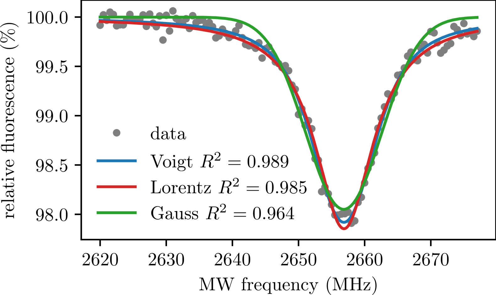
Figure 5: An example of an ODMR resonance fitted with a Gaussian, a Lorentzian, and a Voigt profile. The Voigt profile achieves the highest $R^{2}$ value. Calculating ODMR sensitivities from these fit curves leads to significant differences, i.e., $\eta_{\text{Voigt}}=$2.65\text{\,}\mathrm{\SIUnitSymbolMicro}\mathrm{T}\mathrm{/}\sqrt{\mathrm{Hz}}$$, $\eta_{\text{Lorentz}}=$2.45\pm 0.05\text{\,}\mathrm{\SIUnitSymbolMicro}\mathrm{T}\mathrm{/}\sqrt{\mathrm{Hz}}$$ and $\eta_{\text{Gauss}}=$3.05\pm 0.08\text{\,}\mathrm{\SIUnitSymbolMicro}\mathrm{T}\mathrm{/}\sqrt{\mathrm{Hz}}$$. The Lorentz fit in this example overestimates the actual sensitivity by more than $8\text{\,}\mathrm{\char 37\relax}$.

The Voigt profile can be expressed by the real part of the Faddeeva function [44, 45, 46]

$$\omega(z)=e^{-z^{2}}\text{erfc}(-iz),$$ (23)

which is readily available in commonly used programming languages like Python [47] and MATLAB [48]. The fit model is then written as

$$V(f)=1-\frac{\text{Re}[\omega(z)]}{\sigma\sqrt{2\pi}},\enspace\text{with}\enspace z=\frac{f-f_{\text{res}}+i\nu}{\sigma\sqrt{2}},$$ (24)

with $\nu$ and $\sigma$ as width parameters for the Lorentzian and Gaussian parts, respectively. In lock-in amplified measurements using frequency modulation, the derivative of the ODMR signal is recorded instead, and the fit model becomes

$$\frac{\partial V(f)}{\partial f}=-\frac{1}{\sigma^{3}\sqrt{2\pi}}\left(\nu\text{Im}[\omega(z)]-(f-f_{\text{res}})\text{Re}[\omega(z)]\right).$$ (25)

The magnetic-field sensitivity depends on the maximum value of the derivative of the ODMR signal and the photon-collection rate $P$

$$\eta=\frac{1}{\gamma_{\text{NV}}}\frac{1}{\text{max}\left|\frac{\partial V(f)}{\partial f}\right|}\frac{1}{\sqrt{P}}.$$ (26)

The FWHM linewidths of the Lorentzian and the Gaussian part of the model are retrieved by

$$\alpha_{\text{G}} =2\sigma\sqrt{2\ln 2},$$ (27)

$$\alpha_{\text{L}} =2\nu.$$ (28)

The only inconvenience of using the Voigt profile as a fit model is that the total FWHM linewidth $\alpha_{\text{V}}$ is not trivial to calculate. However, simple-to-use numerical approximations [49, 50, 51] like

$$\alpha_{\text{V}}\approx 0.5346\alpha_{\text{L}}+\sqrt{0.2166\alpha_{\text{L}}^{2}+\alpha_{\text{G}}^{2}}.$$ (29)

exist, that are sufficiently accurate (relative error $<0.025\text{\,}\mathrm{\char 37\relax}$). With the Voigt profile, we can describe the line broadening due to MW power saturation with the dimensionless coordinate [49]

$$d=\frac{\alpha_{\text{L}}-\alpha_{\text{G}}}{\alpha_{\text{L}}+\alpha_{\text{G}}}\enspace\in[-1,1].$$ (30)

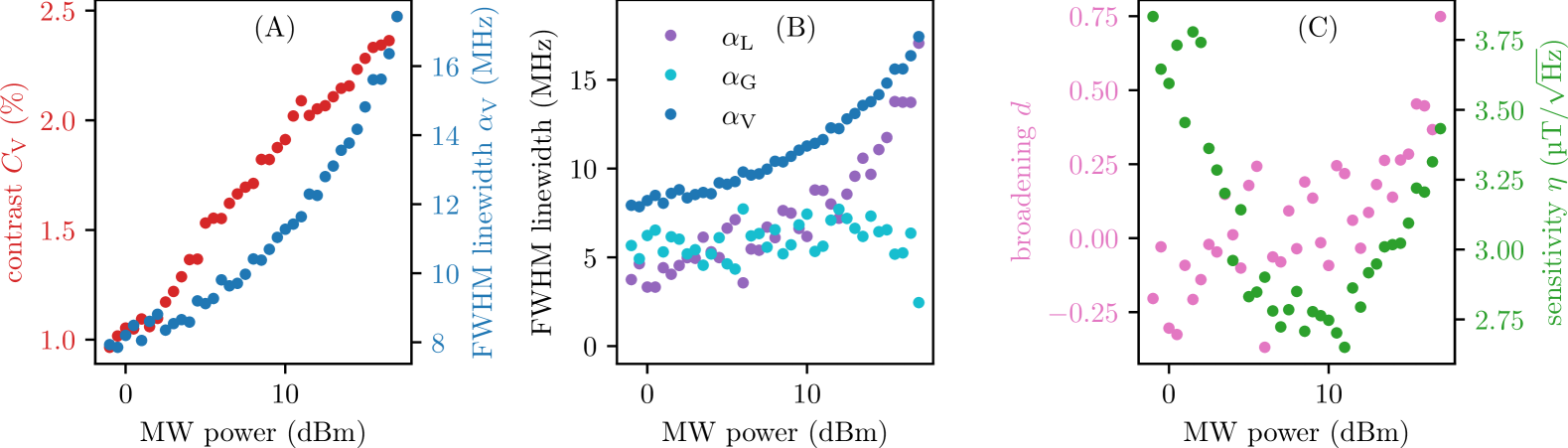
Figure 6: Voigt fit parameters describing the power broadening of the example ODMR peak shown in Figure 5. (A) Both contrast and FWHM linewidth increase with higher MW power, but it is unclear which MW power would lead to an optimal magnetic-field sensitivity. (B) The individual linewidths of the Lorentzian and the Gaussian part of the Voigt fit indicate how far the power broadening increases the total linewidth. For higher MW powers, the line shape is shifted to a Lorentzian shape, where $\alpha_{\text{L}}\rightarrow\alpha_{\text{V}}$ and $\alpha_{\text{G}}\rightarrow 0$. (C) The broadening factor $d$ can describe the power broadening, showing the Lorentzian shape again with $d\rightarrow 1$. The magnetic-field sensitivity $\eta$, dependent on contrast and linewidth $(\propto\alpha_{\text{V}}/C_{\text{V}})$, reaches a minimum when the power broadening broadening starts to take effect. In this case, the magnetic-field sensitivity is only in the order of $\text{\,}\mathrm{\SIUnitSymbolMicro T}$ because a diamond with a low nitrogen concentration was used for these ODMR spectra. The nitrogen concentration does not affect the line broadening.

Figure 6 shows the Voigt fitting parameters for an example ODMR resonance with varying MW power. As expected, the contrast of the resonance increases in Figure 6 (A), but so does the linewidth. It is not immediately apparent which MW power will lead to an optimal sensitivity. However, the Voigt fit parameters $\sigma$ and $\nu$ give a good indication of the line broadening in Figure 6 (B), where for large MW powers the Lorentzian part of the linewidth $\alpha_{\text{L}}$ converges to the total linewidth $\alpha_{\text{V}}$, while the Gaussian part of the linewidth $\alpha_{\text{G}}$ decreases towards zero. When we compare the broadening factor $d$ to the sensitivity $\eta$ in Figure 6 (C), we can see that the sensitivity worsens significantly when the broadening factor increases or decreases drastically. A typical and time-consuming procedure to optimize the sensitivity is to sweep the MW power and record multiple ODMR spectra, apply fit curves, calculate the sensitivity, and see which MW power is optimal. A clear benefit of using a Voigt profile is that a single ODMR spectrum is sufficient to calculate the broadening factor $d$ and, therefore, see whether the applied MW power was too low or too high. With this additional information, one can quickly narrow down the right region of MW power for a given laser power.

VI Conclusion

Here, we provided ready-to-use formulas for accurately and analytically solving the NV Hamiltonian for calculating magnetic fields from measured spin-resonance frequencies and predicting the resonance splitting from a given magnetic field. We showed that these formulas are computationally inexpensive to solve, which can drastically improve the readout bandwidth of NV-based magnetometers.

We discussed the uncertainty and limitations of absolute vector magnetometry with NV centers in diamonds by estimating the influence of different measurement uncertainties. We concluded that the uncertainty of absolute magnetometry typically lies in the order of a few $\text{\,}\mathrm{\SIUnitSymbolMicro T}$. The most significant limitation is the uncertainty of the $g_{\text{NV}}$-factor. Additionally, the assumption that the magnetic-field vector is perfectly aligned with the NV axis leads to a significant systematic error, when the magnetic field is even slightly misaligned.

Finally, we reported on the use of the Voigt profile as a fit model for ODMR spectra. We showed that the Voigt profile more accurately fits recorded ODMR spectra than Gaussian or Lorentzian fit models and brings the additional benefit of detecting the MW power broadening from a single ODMR spectrum.

VII Data and code availability

All data shown in the figures are available on Zenodo. The authors published a Python package containing routines to calculate the analytical solutions presented on the Python Package Index (PyPI) [52] in the hope that it will be useful for other people in this field. The code library used to control the devices for all measurements can be found in [53].

VIII Acknowledgements

This project was funded by the Deutsche Forschungsgemeinschaft (DFG, German Research Foundation) Project-ID No. 454931666 and the Quanten-Initiative Rheinland-Pfalz (QUIP).

Appendix A Derivation of formulas for the magnetic-field calculation

We derive Equations (10) and (11) from the characteristic polynomial, which reads

$$0=\det\begin{vmatrix}\lambda-\frac{1}{3}D-\mathcal{B}\cos\theta&-\frac{1}{\sqrt{2}}\mathcal{B}\sin\theta&-E\\ -\frac{1}{\sqrt{2}}\mathcal{B}\sin\theta&\lambda+\frac{2}{3}D&-\frac{1}{\sqrt{2}}\mathcal{B}\sin\theta\\ -E&-\frac{1}{\sqrt{2}}\mathcal{B}\sin\theta&\lambda-\frac{1}{3}D+\mathcal{B}\cos\theta\\ \end{vmatrix}$$ (31)

$$\Rightarrow 0=\lambda^{3}-\left(\frac{1}{3}D^{2}+E^{2}+\mathcal{B}^{2}\right)\lambda\\ -\frac{1}{2}D\mathcal{B}^{2}\cos(2\theta)-\frac{1}{6}D\mathcal{B}^{2}+\frac{2}{27}D^{3}-\frac{1}{2}E\mathcal{B}^{2}\sin^{2}\theta-\frac{2}{3}DE^{2}$$ (32)

Generally, a polynomial of third order with three roots $\lambda_{0},\lambda_{1},\lambda_{2}$ can be written as

$$(\lambda-\lambda_{0})(\lambda-\lambda_{1})(\lambda-\lambda_{2})=\\ \lambda^{3}-(\lambda_{0}+\lambda_{1}+\lambda_{2})\lambda^{2}+(\lambda_{0}\lambda_{1}+\lambda_{1}\lambda_{2}+\lambda_{0}\lambda_{2})\lambda-\lambda_{0}\lambda_{1}\lambda_{2}$$ (33)

We define the resonance frequencies $f_{\text{u}}$ and $f_{\text{l}}$ in terms of differences between the energy levels

$$\lambda_{0}=\frac{1}{3}(-f_{\text{u}}-f_{\text{l}}),\quad\lambda_{1}=\frac{2}{3}(f_{\text{l}}-f_{\text{u}}),\quad\lambda_{2}=\frac{2}{3}(f_{\text{u}}-f_{\text{l}}),$$ (34)

so that $f_{\text{u}}=\lambda_{2}-\lambda_{0}$ and $f_{\text{l}}=\lambda_{1}-\lambda_{0}$ and the sum of all roots vanishes $\lambda_{0}+\lambda_{1}+\lambda_{2}=0$ as expected.

The linear term of the characteristic polynomial has to fulfill

$$p=\lambda_{0}\lambda_{1}+\lambda_{1}\lambda_{2}+\lambda_{0}\lambda_{2}\\ \Rightarrow-\left(\frac{1}{3}D^{2}+E^{2}+\mathcal{B}^{2}\right)=-\frac{1}{3}(f_{\text{u}}^{2}+f_{\text{l}}^{2}-f_{\text{u}}f_{\text{l}})\\ \Rightarrow\mathcal{B}^{2}=\frac{1}{3}(f_{\text{u}}^{2}+f_{\text{l}}^{2}-f_{\text{u}}f_{\text{l}}-D^{2}-3E^{2})\enspace\square$$ (35)

Additionally, the constant term of the characteristic polynomial has to fulfill

$$q=-\lambda_{0}\lambda_{1}\lambda_{2}\\ \Rightarrow-\frac{1}{2}D\mathcal{B}^{2}\cos(2\theta)-\frac{1}{6}D\mathcal{B}^{2}+\frac{2}{27}D^{3}-\frac{1}{2}E\mathcal{B}^{2}\sin^{2}\theta-\frac{2}{3}DE^{2}\\ =\frac{-2f_{\text{l}}^{3}+3f_{\text{l}}^{2}f_{\text{u}}+3f_{\text{l}}f_{\text{u}}^{2}-2f_{\text{u}}^{3}}{27}.$$ (36)

Sorting all $\theta$ to the left and using the expanded cosine form $\frac{1}{2}D\cos(2\theta)+\frac{1}{2}E\sin^{2}\theta=-\frac{1}{2}D+\frac{1}{2}E+D\cos^{2}\theta-\frac{1}{2}E\cos^{2}\theta$ leads to

$$\Rightarrow\cos^{2}\theta=\frac{2f_{\text{l}}^{3}-3f_{\text{l}}^{2}f_{\text{u}}-3f_{\text{l}}f_{\text{u}}^{2}+2f_{\text{u}}^{3}}{27(D-E/2)\mathcal{B}^{2}}\\ +\frac{2D^{3}-18DE^{2}}{27(D-E/2)\mathcal{B}^{2}}+\frac{2D-3E}{6(D-E/2)}\enspace\square$$ (37)

Appendix B Calibration of the diamond orientation in our setup

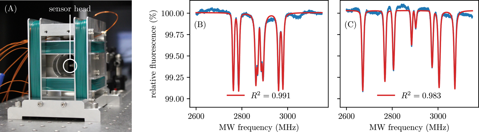
Figure 7: (A) The sensor previously presented in Reference [54] was used to record the ODMR spectra shown in Figure 1. We recorded two additional spectra used for calibration when (B) only the $y$-coil is turned on with $4\text{\,}\mathrm{A}$ and (C) only the $z$-coil is turned on with $4\text{\,}\mathrm{A}$ coil current. We find that the calculated magnetic-field vectors of these two spectra are not perfectly aligned at a $90\text{\,}\mathrm{\SIUnitSymbolDegree}$ angle. We reason that this alignment error of our coil system is the cause for the slight discrepancies between the theory curves and the measured resonance frequencies in Figure 1 (B).

In the experiment setup used to measure the ODMR spectra for Figure 1, we do not know the orientation of the diamond on our sensor. We need one calibration measurement first to calculate the orientation of the diamond. For the measurement in Figure 1 (A), where the magnetic field direction is fixed and the coil current is varied, we chose the ODMR spectrum with maximal field strength as the calibration measurement. The theory curves are then calculated by keeping the four angles to the NV axes constant and varying the absolute value of the magnetic field.

For the measurement in Figure 1 (B), we first recorded two ODMR spectra shown in Figure 7 with only the $z$-coil and the $y$-coil turned on, respectively. From these spectra, we calculate the magnetic-field vectors of the $y$- and $z$-coil using Equation (14) as

$$\vec{B}_{y\text{-coil}} =$1.03\text{\,}\mathrm{mT}$\begin{pmatrix}0.74\\ 0.66\\ 0.14\\ \end{pmatrix}$$ (38)

$$\vec{B}_{z\text{-coil}} =$1.90\text{\,}\mathrm{mT}$\begin{pmatrix}0.81\\ 0.47\\ 0.34\\ \end{pmatrix}$$ (39)

per $1\text{\,}\mathrm{A}$ coil current. For the shown measurement, the coil currents were scaled accordingly so that the absolute magnetic-field value stays constant during the rotation of the field vector. Each one of these two vectors could be expanded with the $\text{O}_{\text{h}}$ symmetry, but we have the additional information that both vectors should have a $90\text{\,}\mathrm{\SIUnitSymbolDegree}$ angle between them. However, when comparing all possible vector solutions, the best matching vectors have an angle of $\approx 98\text{\,}\mathrm{\SIUnitSymbolDegree}$. This discrepancy is likely due to uneven coil windings or slight alignment deviations of the two coils. We reason that this is the cause for the slight discrepancies between the theory curves and the measured resonance frequencies. Nonetheless, we rotate our coordinate system so that the $y$-coil and $z$-coil field vectors are as best aligned with the laboratory frame’s $y$- and $z$-axes as possible. With this rotation, we then calculate the angle-dependent theory curves.

Appendix C Symmetry of the solutions of absolute vector magnetometry

The 48 transformation matrices of the $\text{O}_{\text{h}}$ symmetry group are derived from the six $3\times 3$ permutation matrices with all $2^{3}$ possible sign combinations

$$\begin{pmatrix}\pm 1&0&0\\ 0&\pm 1&0\\ 0&0&\pm 1\\ \end{pmatrix},\enspace\begin{pmatrix}0&\pm 1&0\\ 0&0&\pm 1\\ \pm 1&0&0\\ \end{pmatrix},\enspace\begin{pmatrix}0&0&\pm 1\\ \pm 1&0&0\\ 0&\pm 1&0\\ \end{pmatrix},$$ (40)

$$\begin{pmatrix}0&\pm 1&0\\ \pm 1&0&0\\ 0&0&\pm 1\\ \end{pmatrix},\enspace\begin{pmatrix}0&0&\pm 1\\ 0&\pm 1&0\\ \pm 1&0&0\\ \end{pmatrix},\enspace\begin{pmatrix}\pm 1&0&0\\ 0&0&\pm 1\\ 0&\pm 1&0\\ \end{pmatrix}.$$ (41)

Appendix D Computation benchmarks

In Figure 4, each of the $600\text{\,}$ data points consists of an average over $500\text{\,}$ runs. Benchmarks are written in Python 3.12.0 using the timeit package and were run on an Intel i3-12100 processor on Windows 11, version 23H2. Enabling or disabling Python’s Garbage Collector did not affect any results.

The benchmark for the numerical approach is implemented as follows, similar to [33]. An initial guess of a magnetic-field vector is rotated onto the four diamond-lattice axes. With these rotated vectors, the four Hamiltonians for each axis are computed numerically with the numpy.linalg.eigvalsh function of the Python numpy package [55]. The SSR between the calculated and the measured resonance frequencies is then minimized by a gradient-descent algorithm that iteratively adjusts the input magnetic-field vector. The code for both Benchmarks can be found on Zenodo.

References

- Barry et al. [2020] J. F. Barry, J. M. Schloss, E. Bauch, M. J. Turner, C. A. Hart, L. M. Pham, and R. L. Walsworth, Sensitivity optimization for NV-diamond magnetometry, Reviews of Modern Physics 92, 015004 (2020).
- Aslam et al. [2023] N. Aslam, H. Zhou, E. K. Urbach, M. J. Turner, R. L. Walsworth, M. D. Lukin, and H. Park, Quantum sensors for biomedical applications, Nature Reviews Physics 5, 157 (2023).
- Segawa and Igarashi [2023] T. F. Segawa and R. Igarashi, Nanoscale quantum sensing with Nitrogen-Vacancy centers in nanodiamonds – A magnetic resonance perspective, Progress in Nuclear Magnetic Resonance Spectroscopy 134-135, 20 (2023).
- Scholten et al. [2021] S. C. Scholten, A. J. Healey, I. O. Robertson, G. J. Abrahams, D. A. Broadway, and J.-P. Tetienne, Widefield quantum microscopy with nitrogen-vacancy centers in diamond: Strengths, limitations, and prospects, Journal of Applied Physics 130, 150902 (2021).
- Doherty et al. [2013] M. W. Doherty, N. B. Manson, P. Delaney, F. Jelezko, J. Wrachtrup, and L. C. Hollenberg, The nitrogen-vacancy colour centre in diamond, Physics Reports 528, 1 (2013).
- Gruber et al. [1997] A. Gruber, A. Dräbenstedt, C. Tietz, L. Fleury, J. Wrachtrup, and C. V. Borczyskowski, Scanning Confocal Optical Microscopy and Magnetic Resonance on Single Defect Centers, Science 276, 2012 (1997).
- Degen [2008] C. L. Degen, Scanning magnetic field microscope with a diamond single-spin sensor, Applied Physics Letters 92, 243111 (2008).
- Doherty et al. [2011] M. W. Doherty, N. B. Manson, P. Delaney, and L. C. L. Hollenberg, The negatively charged nitrogen-vacancy centre in diamond: the electronic solution, New Journal of Physics 13, 025019 (2011).
- Rondin et al. [2014] L. Rondin, J.-P. Tetienne, T. Hingant, J.-F. Roch, P. Maletinsky, and V. Jacques, Magnetometry with nitrogen-vacancy defects in diamond, Reports on Progress in Physics 77, 056503 (2014).
- Loubser and Wyk [1978] J. H. N. Loubser and J. A. V. Wyk, Electron spin resonance in the study of diamond, Reports on Progress in Physics 41, 1201 (1978).
- Schloss et al. [2018] J. M. Schloss, J. F. Barry, M. J. Turner, and R. L. Walsworth, Simultaneous Broadband Vector Magnetometry Using Solid-State Spins, Physical Review Applied 10, 034044 (2018).
- Barry et al. [2024] J. F. Barry, M. H. Steinecker, S. T. Alsid, J. Majumder, L. M. Pham, M. F. O’Keeffe, and D. A. Braje, Sensitive ac and dc magnetometry with nitrogen-vacancy-center ensembles in diamond, Physical Review Applied 22, 044069 (2024).
- Wolf et al. [2015] T. Wolf, P. Neumann, K. Nakamura, H. Sumiya, T. Ohshima, J. Isoya, and J. Wrachtrup, Subpicotesla Diamond Magnetometry, Physical Review X 5, 041001 (2015).
- Xie et al. [2021] Y. Xie, H. Yu, Y. Zhu, X. Qin, X. Rong, C.-K. Duan, and J. Du, A hybrid magnetometer towards femtotesla sensitivity under ambient conditions, Science Bulletin 66, 127 (2021).
- Wang et al. [2022] Z. Wang, F. Kong, P. Zhao, Z. Huang, P. Yu, Y. Wang, F. Shi, and J. Du, Picotesla magnetometry of microwave fields with diamond sensors, Science Advances 8, eabq8158 (2022).
- Hu et al. [2024] Z.-G. Hu, Y.-M. Gao, J.-F. Liu, H. Yang, M. Wang, Y. Lei, X. Zhou, J. Li, X. Cao, J. Liang, C.-Q. Hu, Z. Li, Y.-C. Lau, J.-W. Cai, and B.-B. Li, Picotesla-sensitivity microcavity optomechanical magnetometry, Light: Science & Applications 13, 279 (2024).
- Yamaguchi et al. [2019] T. Yamaguchi, Y. Matsuzaki, S. Saito, S. Saijo, H. Watanabe, N. Mizuochi, and J. Ishi-Hayase, Bandwidth analysis of AC magnetic field sensing based on electronic spin double-resonance of nitrogen-vacancy centers in diamond, Japanese Journal of Applied Physics 58, 100901 (2019).
- Doherty et al. [2012] M. W. Doherty, F. Dolde, H. Fedder, F. Jelezko, J. Wrachtrup, N. B. Manson, and L. C. L. Hollenberg, Theory of the ground-state spin of the NV- center in diamond, Physical Review B 85, 205203 (2012).
- Press et al. [2007] W. H. Press, S. A. Teukolsky, W. T. Vetterling, and B. P. Flannery, Numerical Recipes - The Art of Scientific Computing - 3rd Edition (Cambridge University Press, 2007).
- Viète [1646] F. Viète, Opera Mathematica in unum volumen congesta (Bonaventure & Abraham Elzevier, Leiden, 1646).
- Wolters [2021] D. J. Wolters, Practical Algorithms for solving the Cubic Equation, (2021).
- Nickalls [2006] R. W. D. Nickalls, Viète, Descartes and the cubic equation, The Mathematical Gazette 90, 203 (2006).
- Lee et al. [2015] S.-Y. Lee, M. Niethammer, and J. Wrachtrup, Vector magnetometry based on electronic spins, Physical Review B 92, 115201 (2015).
- Balasubramanian et al. [2008] G. Balasubramanian, I. Y. Chan, R. Kolesov, M. Al-Hmoud, J. Tisler, C. Shin, C. Kim, A. Wojcik, P. R. Hemmer, A. Krueger, T. Hanke, A. Leitenstorfer, R. Bratschitsch, F. Jelezko, and J. Wrachtrup, Nanoscale imaging magnetometry with diamond spins under ambient conditions, Nature 455, 648 (2008).
- Ye et al. [2019] J.-F. Ye, Z. Jiao, K. Ma, Z.-Y. Huang, H.-J. Lv, and F.-J. Jiang, Reconstruction of vector static magnetic field by different axial NV centers using continuous wave optically detected magnetic resonance in diamond, Chinese Physics B 28, 047601 (2019).
- Weggler et al. [2020] T. Weggler, C. Ganslmayer, F. Frank, T. Eilert, F. Jelezko, and J. Michaelis, Determination of the Three-Dimensional Magnetic Field Vector Orientation with Nitrogen Vacany Centers in Diamond, Nano Letters 20, 2980 (2020).
- Aitken [1936] A. Aitken, On Least Squares and Linear Combination of Observations, Proceedings of the Royal Society of Edinburgh 10.1017/S0370164600014346 (1936).
- Beaver et al. [2024] N. M. Beaver, N. Voce, P. Meisenheimer, R. Ramesh, and P. Stevenson, Optimizing off-axis fields for two-axis magnetometry with point defects, Applied Physics Letters 124, 254001 (2024).
- Silani et al. [2023] Y. Silani, J. Smits, I. Fescenko, M. W. Malone, A. F. McDowell, A. Jarmola, P. Kehayias, B. A. Richards, N. Mosavian, N. Ristoff, and V. M. Acosta, Nuclear quadrupole resonance spectroscopy with a femtotesla diamond magnetometer, Science Advances 9, eadh3189 (2023).
- Simin et al. [2015] D. Simin, F. Fuchs, H. Kraus, A. Sperlich, P. Baranov, G. Astakhov, and V. Dyakonov, High-Precision Angle-Resolved Magnetometry with Uniaxial Quantum Centers in Silicon Carbide, Physical Review Applied 4, 014009 (2015).
- Maertz et al. [2010] B. J. Maertz, A. P. Wijnheijmer, G. D. Fuchs, M. E. Nowakowski, and D. D. Awschalom, Vector magnetic field microscopy using nitrogen vacancy centers in diamond, Applied Physics Letters 96, 092504 (2010).
- Steinert et al. [2010] S. Steinert, F. Dolde, P. Neumann, A. Aird, B. Naydenov, G. Balasubramanian, F. Jelezko, and J. Wrachtrup, High sensitivity magnetic imaging using an array of spins in diamond, Review of Scientific Instruments 81, 043705 (2010).
- Garsi et al. [2024] M. Garsi, R. Stöhr, A. Denisenko, F. Shagieva, N. Trautmann, U. Vogl, B. Sene, F. Kaiser, A. Zappe, R. Reuter, and J. Wrachtrup, Three-dimensional imaging of integrated-circuit activity using quantum defects in diamond, Physical Review Applied 21, 014055 (2024).
- Tsukamoto et al. [2022] M. Tsukamoto, S. Ito, K. Ogawa, Y. Ashida, K. Sasaki, and K. Kobayashi, Accurate magnetic field imaging using nanodiamond quantum sensors enhanced by machine learning, Scientific Reports 12, 13942 (2022).
- Homrighausen et al. [2023] J. Homrighausen, L. Horsthemke, J. Pogorzelski, S. Trinschek, P. Glösekötter, and M. Gregor, Edge-Machine-Learning-Assisted Robust Magnetometer Based on Randomly Oriented NV-Ensembles in Diamond, Sensors 23, 1119 (2023).
- Zhang et al. [2024] E. Zhang, W. Zhang, X. Jiang, and X. Qin, Deep-neural-network-based magnetic-field acquisition method for quantum sensing with nitrogen-vacancy centers, Physical Review A 110, 052417 (2024).
- Tiesinga et al. [2021] E. Tiesinga, P. J. Mohr, D. B. Newell, and B. N. Taylor, CODATA recommended values of the fundamental physical constants: 2018, Reviews of Modern Physics 93, 025010 (2021).
- He et al. [1993] X.-F. He, N. B. Manson, and P. T. H. Fisk, Paramagnetic resonance of photoexcited N- V defects in diamond. I. Level anticrossing in the 3 A ground state, Physical Review B 47, 8809 (1993).
- Felton et al. [2009] S. Felton, A. M. Edmonds, M. E. Newton, P. M. Martineau, D. Fisher, D. J. Twitchen, and J. M. Baker, Hyperfine interaction in the ground state of the negatively charged nitrogen vacancy center in diamond, Physical Review B 79, 075203 (2009).
- Homrighausen et al. [2024] J. Homrighausen, F. Hoffmann, J. Pogorzelski, P. Glösekötter, and M. Gregor, Microscale fiber-integrated vector magnetometer with on-tip field biasing using N - V ensembles in diamond microcrystals, Physical Review Applied 22, 034029 (2024).
- Dréau et al. [2011] A. Dréau, M. Lesik, L. Rondin, P. Spinicelli, O. Arcizet, J.-F. Roch, and V. Jacques, Avoiding power broadening in optically detected magnetic resonance of single NV defects for enhanced dc magnetic field sensitivity, Physical Review B 84, 195204 (2011).
- Citron et al. [1977] M. L. Citron, H. R. Gray, C. W. Gabel, and C. R. Stroud, Experimental study of power broadening in a two-level atom, Physical Review A 16, 1507 (1977).
- Vitanov et al. [2001] N. Vitanov, B. Shore, L. Yatsenko, K. Böhmer, T. Halfmann, T. Rickes, and K. Bergmann, Power broadening revisited: theory and experiment, Optics Communications 199, 117 (2001).
- Shippony and Read [1993] Z. Shippony and W. Read, A highly accurate Voigt function algorithm, Journal of Quantitative Spectroscopy and Radiative Transfer 50, 635 (1993).
- Shippony and Read [2003] Z. Shippony and W. Read, A correction to a highly accurate Voigt function algorithm, Journal of Quantitative Spectroscopy and Radiative Transfer 78, 255 (2003).
- Weideman [1994] J. A. C. Weideman, Computation of the Complex Error Function, SIAM Journal on Numerical Analysis 31, 1497 (1994).
- noa [2025a] Scipy faddeeva function (2025a), (visited on 29th April 2025).
- [48] S. G. Johnson, MATLAB Faddeeva package, (visited on 29th April 2025).
- Olivero and Longbothum [1977] J. Olivero and R. Longbothum, Empirical fits to the Voigt line width: A brief review, Journal of Quantitative Spectroscopy and Radiative Transfer 17, 233 (1977).
- Whiting [1968] E. Whiting, An empirical approximation to the Voigt profile, Journal of Quantitative Spectroscopy and Radiative Transfer 8, 1379 (1968).
- Kielkopf [1973] J. F. Kielkopf, New approximation to the Voigt function with applications to spectral-line profile analysis, J. Opt. Soc. Am. 63, 987 (1973).
- [52] D. Lönard, I. C. Barbosa, S. Johansson, A. Erlenbach, J. Gutsche, and A. Widera, Python nvtools, (visited on 29th April 2025).
- Lönard et al. [2025] D. Lönard, I. C. Barbosa, S. Johansson, A. Erlenbach, J. Gutsche, and A. Widera, Microscope Experiment Control Application (2025).
- Dix et al. [2024] S. Dix, D. Lönard, I. C. Barbosa, J. Gutsche, J. Witzenrath, and A. Widera, A miniaturized magnetic field sensor based on nitrogen-vacancy centers (2024), arXiv:2402.19372 [physics].
- noa [2025b] Numpy eigvalsh (2025b), (visited on 29th April 2025).