Unimodality of the number of paths per length on polytopes
Examples, counter-examples, and central limit theorem

Abstract

To solve a linear program, the simplex method follows a path in the graph of a polytope, on which a linear function increases. The length of this path is an key measure of the complexity of the simplex method. Numerous previous articles focused on the longest paths, or, following Borgwardt, computed the average length of a path for certain random polytopes. We detail more precisely how this length is distributed, i.e., how many paths of each length there are.

It was conjectured by De Loera that the number of paths counted according to their length forms a unimodal sequence. We give examples (old and new) for which this holds; but we disprove this conjecture by constructing counterexamples for several classes of polytopes. However, De Loera is “statistically correct”: We prove that the length of coherent paths on a random polytope (with vertices chosen uniformly on a sphere) admits a central limit theorem.

1 Introduction

For a polytope $\mathsf{P}\subset\mathbb{R}^{d}$ and a direction ${\boldsymbol{c}}\in\mathbb{R}^{d}$, one can wonder about the monotone paths on $\mathsf{P}$: the paths in the graph of $\mathsf{P}$ along which the scalar product against ${\boldsymbol{c}}$ increases. How many monotone paths are there? What are the lengths of these paths? Are there more short paths, more long paths, or more paths of almost average length?

Not only are theses questions natural to ask, but in addition, they are also of prime importance in several contexts. First and foremost, to solve a linear program using the famous simplex method introduced by Dantzig in 1947 (see [17]), one traverses such a path. Hence, the length of monotone paths is a key measure of the complexity of the simplex method. Following Klee and Minty [22] seminal example of a polytope with $m$ facets and monotone paths of length exponential in $m$, numerous researches were led both on classes of polytopes with very long or very short longest paths, and on the expected length of a monotone path on random polytopes. As the literature on the subject is endless, we restrict to some pointers that the reader might find useful. Especially, [2] studies the number of monotone paths on polytopes, while [3] focuses on the connectivity of the graph of paths (where a path can be “flipped” into another by switching its behavior around a 2-face). Besides, [7] presents some results on extremal lengths of monotone paths for specific classes of polytopes, and [6] addresses the case of zonotopes.

On a more combinatorial side, when the graph of $\mathsf{P}$ (directed along ${\boldsymbol{c}}$) embodies a lattice, then the monotone paths are the maximal chains of this lattice. Nelson [30] unraveled monotone paths on the associahedron (i.e., maximal chains in the Tamari lattice), while [19] extended this exploration to graph associahedra. As of monotone paths on the permutahedron, they are renown under the name of “sorting networks” [4, 18].

The simplex method chooses the monotone path it traverses thanks to a pivot rule: at each vertex, this rule tells you which (${\boldsymbol{c}}$-improving) neighboring vertex will be the next in your path. As the simplex method cares about avoiding long paths, clever pivot rules were proposed to keep us away from “whirling too much” around $\mathsf{P}$. It is a properties of the shadow vertex rule: choose a plane to project $\mathsf{P}$ onto, you will obtain a polygon, then take one of the only two paths on this polygonal projection as your monotone path. Following this idea, a monotone path is coherent if it can be elected by the shadow vertex rule for some plane of projection; equivalently, if there exists a 2-dimensional projection of $\mathsf{P}$ for which this path projects to the boundary of the projection.

In his book [12], Borgwardt analyzed the shadow vertex rule, and especially computed the average length of coherent paths for several classes of random polytopes. Since, numerous authors contributed to the field. In particular, the generalization from coherent paths to coherent subdivisions by Billera and Sturmfels’s construction of fiber polytopes [15] spurred towards new exciting researches on the subject. With this perspective, coherent paths (and monotone path polytopes) where studied on simplices and cubes [15], on cyclic polytopes [5], on $S$-hypersimplices [28], on cross-polytopes [9], on (usual) hypersimplices [31].

Yet, Borgwardt left open various questions regarding the probabilistic behavior of the length of coherent paths. Remarkably, although he computed the expectation for several models of random polytopes, he asked [12, Chapter 0.12, Question 8]: “Is it possible to study the higher probabilistic moments of the distribution of $s$?” ($s$ is the length of a coherent path). Meanwhile, tremendous progress has been made in the theory of random polytopes, in particular in [33, 34, 27, 25, 35]. The literature now offers tools to assess the second moment (i.e., the variance) and to determine the asymptotic form of the distribution (i.e., establish a central limit theorem) of quantities on random polytopes, like their volume or their number of $k$-faces.

The goal of the our paper is to study the number of monotone paths $N_{\ell}$ and coherent paths $N^{\text{coh}}_{\ell}$ of length $\ell$. We want to lift the veil covering the distribution of the sequences $(N_{\ell})_{\ell}$ and $(N^{\text{coh}}_{\ell})_{\ell}$, both for explicit examples of polytopes, and for a natural probabilistic model of random polytopes. Intuitively, one might expect that, for a small (or large) $\ell$, there are only few paths of length $\ell$ (comparing to the total number of paths), but around the average length there are a lot of paths: Indeed, a path can usually be slightly modified to obtain a path of similar length; this modification seems to act like in a Galton board, making the length closer to its mean.

Recall that a sequence of numbers $\mathbf{a}=(a_{1},\dots,a_{r})$ is unimodal if there exists $k\in[r]$ such that $a_{i}\leq a_{i+1}$ for all $i<k$, and $a_{i}\geq a_{i+1}$ for all $i\geq k$, see Figure˜2. Our paper is motivated by:

Question A.

Given a polytope $\mathsf{P}\subset\mathbb{R}^{d}$ and a (generic) direction ${\boldsymbol{c}}\in\mathbb{R}^{d}$, are the sequences $(N_{\ell})_{\ell}$ and $(N_{\ell}^{\text{coh}})_{\ell}$ of the number of monotone and coherent paths, counted according to length, unimodal?

It has been conjectured by Jesús de Loera (personal communication) that this question has an affirmative answer, and this has been confirmed for special instances. On the positive side, we will provide more examples where the answer is “yes”, leading to (see Section˜3 for more details):

Theorem A.

The numbers of monotone and coherent paths, counted per length, are unimodal for:

1. $d$-simplex, for any generic ${\boldsymbol{c}}$;

2. standard $d$-cube, for ${\boldsymbol{c}}=(1,\dots,1)$;

3. $d$-cross-polytope, for any generic ${\boldsymbol{c}}$;

4. cyclic polytopes, for ${\boldsymbol{c}}=(1,0,\dots,0)$;

5. $S$-hypersimplex, for ${\boldsymbol{c}}=(1,\dots,1)$;

6. the prism $\mathsf{P}\times[0,1]$, for $({\boldsymbol{c}},1)$, if the corresponding sequence for $\mathsf{P}$ and ${\boldsymbol{c}}$ is log-concave.

On the negative side, we will show that the answer is “no” in general (Section˜4) by providing specific counterexamples for several classes of polytopes, including simple and simplicial polytopes, as well as generalized permutahedra. More precisely, these results can be summarized as follows:

Theorem B.

For the following classes, there exists polytopes and ${\boldsymbol{c}}$ such that $(N_{\ell})_{\ell}$ is not unimodal:

1. $d$-dimensional polytopes, combinatorially isomorphic to the $d$-cube for $d\geq 3$ (Theorem˜4.5);

2. $3$-dimensional simplicial polytopes (Theorem˜4.7);

3. $5$-dimensional generalized permutahedra (Theorem˜4.11);

4. $5$-dimensional $0$-$1$-polytopes, not combinatorially isomorphic to the $5$-cube (Theorem˜4.15).

Moreover, for the classes $(a)$ and $(c)$, the sequence $(N_{\ell}^{\text{coh}})_{\ell}$ is not unimodal either.

In contrast, we show in Section˜5 that, for random polytopes, ˜A has a some-what positive answer. We do not prove that the answer is “yes with high probability”, but we prove that the length of a coherent path (for random polytopes on the sphere) admits a central limit theorem. We present all probabilistic background in Section˜5, and paste here the precise statement:

Theorem C (Theorem˜5.1).

Let $d\geq 4$ and let ${\boldsymbol{c}},{\boldsymbol{\omega}}\in\mathbb{R}^{d}$ be linearly independent vectors (possibly, randomly chosen). Let $Z_{1},\dots,Z_{n}$ be random independent points, chosen uniformly on the sphere $\mathbb{S}^{d-1}\subset\mathbb{R}^{d}$, and let $\mathsf{P}_{n}=\operatorname{conv}(Z_{1},\dots,Z_{n})$. Then, the length $L_{n}$ of the coherent ${\boldsymbol{c}}$-monotone path captured by ${\boldsymbol{\omega}}$ on $\mathsf{P}_{n}$ follows a central limit theorem (here, the convergence is in distribution):

$$\frac{L_{n}-\mathbb{E}(L_{n})}{\sqrt{\operatorname{Var}(L_{n})}}\xrightarrow[n\to+\infty]{}U,~~~~\text{where }U\sim{\mathcal{N}}(0,1)\text{ is standard normally distributed}$$

Moreover, $\mathbb{E}(L_{n})\sim c\,n^{\frac{1}{d-1}}$, and: $c^{\prime}\,n^{\frac{1}{d-1}-a}\leq\operatorname{Var}(L_{n})\leq c^{\prime\prime}\,(\log n)^{3-\frac{1}{d-1}}\,n^{\frac{1}{d-1}}$ for any $a>0$.

2 Preliminaries

On monotone paths and coherent paths on polytopes

A polytope $\mathsf{P}\subset\mathbb{R}^{d}$ is the convex hull of finitely many points, or equivalently, the bounded intersection of finitely many half-spaces. For ${\boldsymbol{c}}\in\mathbb{R}^{d}$, we let $\mathsf{P}^{{\boldsymbol{c}}}\coloneqq\{{\boldsymbol{x}}\in\mathsf{P}~;~\left<{\boldsymbol{x}},{\boldsymbol{c}}\right>=\max_{{\boldsymbol{y}}\in\mathsf{P}}\left<{\boldsymbol{y}},{\boldsymbol{c}}\right>\}$. A subset $\mathsf{F}\subseteq\mathsf{P}$ is a face of $\mathsf{P}$ if there exists ${\boldsymbol{c}}\in\mathbb{R}^{d}$ such that $\mathsf{F}=\mathsf{P}^{{\boldsymbol{c}}}$. The dimension of a face $\mathsf{F}$ is its affine dimension, i.e., the dimension of the smallest affine sub-space of $\mathbb{R}^{d}$ containing $\mathsf{F}$. By convention, $\varnothing$ is a face of $\mathsf{P}$ of dimension $-1$. The vertices of $\mathsf{P}$ are its faces of dimension 0, while its edges are its faces of dimension 1. We will use the notation $[{\boldsymbol{u}},{\boldsymbol{v}}]$ to denote the line segment (which might or might not be an edge) between two vertices ${\boldsymbol{u}}$ and ${\boldsymbol{v}}$ of $\mathsf{P}$. Note that vertices and edges of $\mathsf{P}$ form a graph in an obvious way.

For ${\boldsymbol{c}}\in\mathbb{R}^{d}$, the directed graph $G_{\mathsf{P},{\boldsymbol{c}}}$ is the directed graph whose vertices are the vertices of $\mathsf{P}$, and where there is a directed edge ${\boldsymbol{u}}\to{\boldsymbol{v}}$ in $G_{\mathsf{P},{\boldsymbol{c}}}$ if $[{\boldsymbol{u}},{\boldsymbol{v}}]$ is an edge of $\mathsf{P}$ satisfying $\left<{\boldsymbol{u}},{\boldsymbol{c}}\right><\left<{\boldsymbol{v}},{\boldsymbol{c}}\right>$. A direction ${\boldsymbol{c}}\in\mathbb{R}^{d}$ is generic with respect to $\mathsf{P}$, if $\left<{\boldsymbol{u}},{\boldsymbol{c}}\right>\neq\left<{\boldsymbol{v}},{\boldsymbol{c}}\right>$ for every edge $[{\boldsymbol{u}},{\boldsymbol{v}}]$ of $\mathsf{P}$. If ${\boldsymbol{c}}$ is generic, then the underlying graph of $G_{\mathsf{P},{\boldsymbol{c}}}$ is the graph of $\mathsf{P}$ itself. In this case, $G_{\mathsf{P},{\boldsymbol{c}}}$ has a unique source and a unique sink, namely, the vertex ${\boldsymbol{v}}_{\min}$ and ${\boldsymbol{v}}_{\max}$ of $\mathsf{P}$ that minimizes and maximizes the value of $\left<{\boldsymbol{x}},{\boldsymbol{c}}\right>$ for ${\boldsymbol{x}}\in\mathsf{P}$, respectively.

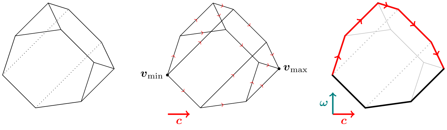
Figure 1: (Left) A $3$-dimensional polytope $\mathsf{P}$; (Middle) The directed graph $G_{\mathsf{P},{\boldsymbol{c}}}$ on which there are 7 monotone paths (3 of length 3, and 2 of length 4, and 2 of length 5); (Right) The projection of $\mathsf{P}$ onto the plane spanned by $({\boldsymbol{c}},{\boldsymbol{\omega}})$ with, in red, the path formed by the upper faces of this projection (another choice of ${\boldsymbol{\omega}}$ would give rise to another coherent path).

Definition 2.1.

For a polytope $\mathsf{P}\subset\mathbb{R}^{d}$ and a direction ${\boldsymbol{c}}\in\mathbb{R}^{d}$, a ${\boldsymbol{c}}$-monotone path is a directed path in $G_{\mathsf{P},{\boldsymbol{c}}}$ from ${\boldsymbol{v}}_{\min}$ to ${\boldsymbol{v}}_{\max}$, see Figure˜1 (Left and middle).

The length of a ${\boldsymbol{c}}$-monotone path is its number of edges, i.e., its number of vertices minus 1. For given $\mathsf{P}$ and ${\boldsymbol{c}}$, we denote by $N_{\ell}(\mathsf{P},{\boldsymbol{c}})$ the number of ${\boldsymbol{c}}$-monotone paths of $\mathsf{P}$ of length $\ell$.

To ease notation and since $\mathsf{P}$ and ${\boldsymbol{c}}$ will be mostly clear from the context (and fixed), we will often just write $N_{\ell}$. Similarly, we will often write “monotone path” instead of ${\boldsymbol{c}}$-monotone path.

Remark 2.2.

Balinski’s theorem ensures that the graph of a $d$-dimensional polytope is $d$-connected. By Menger’s theorem, for any $d$-dimensional polytope there exist at least $d$ (internally disjoint) ${\boldsymbol{c}}$-monotone paths, for all ${\boldsymbol{c}}$. Thus, the number of ${\boldsymbol{c}}$-monotone paths is at least $d$, i.e., $\sum_{\ell}N_{\ell}\geq d$.

Definition 2.3.

Let $\mathsf{P}\subset\mathbb{R}^{d}$ be a polytope and ${\boldsymbol{c}}\in\mathbb{R}^{d}$ a direction. Let ${\boldsymbol{\omega}}\in\mathbb{R}^{d}$ a secondary direction linearly independent from ${\boldsymbol{c}}$, and let $\mathsf{P}_{{\boldsymbol{c}},{\boldsymbol{\omega}}}$ be the polygon obtained by projecting $\mathsf{P}$ onto the plane spanned by ${\boldsymbol{c}}$ and ${\boldsymbol{\omega}}$, that is (see Figure˜1, Right):

$$\mathsf{P}~~\xmapsto{~~\pi_{{\boldsymbol{c}},{\boldsymbol{\omega}}}~~}~~\mathsf{P}_{{\boldsymbol{c}},{\boldsymbol{\omega}}}\coloneqq\Bigl{\{}\bigl{(}\left<{\boldsymbol{x}},{\boldsymbol{c}}\right>,\left<{\boldsymbol{x}},{\boldsymbol{\omega}}\right>\bigr{)}~;~{\boldsymbol{x}}\in\mathsf{P}\Bigr{\}}$$

A proper face (i.e., vertex or edge) $\mathsf{F}$ of $\mathsf{P}_{{\boldsymbol{c}},{\boldsymbol{\omega}}}$ is an upper face if it has an outer normal vector with positive second coordinate, equivalently if $(x_{1},x_{2})+(0,\varepsilon)\notin\mathsf{P}_{{\boldsymbol{c}},{\boldsymbol{\omega}}}$ for all $(x_{1},x_{2})\in\mathsf{F}$, and all $\varepsilon>0$.

A ${\boldsymbol{c}}$-monotone path ${\mathcal{L}}$ on $\mathsf{P}$ is coherent if the projected path $\pi_{{\boldsymbol{c}},{\boldsymbol{\omega}}}({\mathcal{L}})$ is the upper path of $\mathsf{P}_{{\boldsymbol{c}},{\boldsymbol{\omega}}}$ for some ${\boldsymbol{\omega}}\in\mathbb{R}^{d}$, that is to say if there exists ${\boldsymbol{\omega}}\in\mathbb{R}^{d}$ such that ${\mathcal{L}}$ is the family of pre-images by $\pi_{{\boldsymbol{c}},{\boldsymbol{\omega}}}$ of the upper faces of $\mathsf{P}_{{\boldsymbol{c}},{\boldsymbol{\omega}}}$. In this case, such an ${\boldsymbol{\omega}}$ is said to capture the coherent path ${\mathcal{L}}$.

The length of a coherent path is its length as a monotone path. We denote by $N^{\text{coh}}_{\ell}(\mathsf{P},{\boldsymbol{c}})$ the number of coherent paths of length $\ell$. We will just write $N^{\text{coh}}_{\ell}$ when $\mathsf{P}$ and ${\boldsymbol{c}}$ are clearly identified.

Remark 2.4.

By definition, there are fewer coherent than monotone paths of length $\ell$: $N^{\text{coh}}_{\ell}\leq N_{\ell}$.

In addition, every ${\boldsymbol{\omega}}\in\mathbb{R}^{d}$ gives rise to a coherent path ${\mathcal{L}}_{{\boldsymbol{\omega}}}$. Moreover, since ${\mathcal{L}}_{{\boldsymbol{\omega}}}$ is the pre-image of the upper faces of $\mathsf{P}_{{\boldsymbol{c}},{\boldsymbol{\omega}}}$ while ${\mathcal{L}}_{-{\boldsymbol{\omega}}}$ is the pre-image of the lower faces of $\mathsf{P}_{{\boldsymbol{c}},{\boldsymbol{\omega}}}$ by $\pi_{{\boldsymbol{c}},{\boldsymbol{\omega}}}$, the coherent paths ${\mathcal{L}}_{{\boldsymbol{\omega}}}$ and ${\mathcal{L}}_{-{\boldsymbol{\omega}}}$ are internally disjoint from each other. Consequently, $\sum_{\ell}N^{\text{coh}}_{\ell}\geq 2$.

On tools around unimodality

In this subsection, we gather several tools to prove unimodality. We do not intend to provide a handbook on neither unimodality nor log-concavity, and refer the interested reader to e.g., [13].

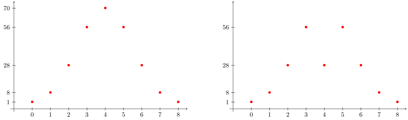
Figure 2: (Left) The sequence of binomial coefficients $\binom{8}{0},\dots,\binom{8}{8}$ is unimodal, symmetric, and also (ultra-)log-concave: its mode is at $4$, its peak is $70$; (Right) A non-unimodal symmetric sequence.

Let $\mathbf{a}=(a_{1},\dots,a_{r})\in\mathbb{N}^{r}$ be a sequence of non-negative integers. The sequence $\mathbf{a}$ is log-concave if $a_{i-1}a_{i+1}\leq a_{i}^{2}$ for all $2\leq i\leq r-1$. The sequence $\mathbf{a}$ is ultra-log-concave if the sequence $\left(\frac{a_{i}}{\binom{r}{i}}\right)_{1\leq i\leq r}$ is log-concave: that is, if $(i+1)(r-i+1)\,a_{i-1}a_{i+1}\leq i(r-i)\,a_{i}^{2}$ for all $2\leq i\leq r-1$. The sequence $\mathbf{a}$ is symmetric if $a_{r-i}=a_{i}$ for all $i\in[r]$.

Any (not necessarily unique) index $k$ is a mode of $\mathbf{a}$ if $a_{k}=\max\mathbf{a}$.

It is well-known and easy to verify that we have the following chain of implications:

$$\mathbf{a}\text{ ulra-log-concave}\,\Rightarrow\,\mathbf{a}\text{ log-concave}\,\Rightarrow\,\mathbf{a}\text{ unimodal}$$

An example of a sequence that is symmetric and ultra-log-concave (and hence, log-concave and unimodal) is provided by the binomial coefficients $(\binom{n}{i}~;~i\in[n])$, see Figure˜2 (Left).

We collect some results on log-concavity and unimodality that we will use. We can (and will) always assume that the sequences at stake have the same lengths, by appending $0$s. We omit the proofs since these statements are well-known, and easily deduced from the definitions.

Lemma 2.5.

Let $\mathbf{a}^{(1)}=(a^{(1)}_{i})_{i\in[r]},\ldots,\mathbf{a}^{(m)}=(a^{(m)}_{i})_{i\in[r]}$ be sequences of non-negative integers.

1. If $\mathbf{a}^{(1)},\ldots,\mathbf{a}^{(m)}$ are log-concave, then so is their product $(a^{(1)}_{i}\cdots a^{(m)}_{i})_{i\in[r]}$.

2. If $\mathbf{a}$ is unimodal and symmetric, then its modes are $\left\lfloor\frac{r+1}{2}\right\rfloor$ and $\left\lceil\frac{r+1}{2}\right\rceil$ (coinciding for $r$ odd).

3. If $\mathbf{a}^{(1)},\ldots,\mathbf{a}^{(m)}$ are unimodal sequences with the same mode, then their sum $\left(\sum_{j=1}^{m}a^{(j)}_{i}\right)_{i\in[r]}$ is unimodal with the same mode.

4. If $\mathbf{a}^{(1)}$ and $\mathbf{a}^{(2)}$ are unimodal with respective modes $k$ and $k+1$, then their sum $(a_{i}^{(1)}+a_{i}^{(2)})_{i\in[r]}$ is unimodal with mode either $k$ or $k+1$.

3 Positive examples

The aim of this section is to provide examples for which ˜A has a positive answer, i.e., for which the sequences $(N_{\ell})_{\ell}$ and $(N^{\text{coh}}_{\ell})_{\ell}$ are unimodal. This includes previously known examples, and additional examples we found. All the sequences $(N_{\ell})_{\ell}$ and $(N^{\text{coh}}_{\ell})_{\ell}$ presented in this section will be proven to be unimodal, except in Examples˜3.8 and 3.10 (where it is only conjectured).

We start by reviewing some cases where the number of monotone paths and/or coherent paths is known. First, we recall the definitions of some polytopes.

polytope	notation	definition
$d$-simplex	$\mathsf{\Delta}_{d}$	convex hull of $d+1$ affinely independent points
standard $d$-cube	$[0,1]^{d}$	$[0,1]^{d}$
$d$-cross-polytope	$\Diamond_{d}$	$\operatorname{conv}(\pm{\boldsymbol{e}}_{i}~;~1\leq i\leq d)$ with ${\boldsymbol{e}}_{i}$ the $i$-th unit vector in $\mathbb{R}^{d}$
cyclic polytope	$\mathsf{Cyc}_{d}({\boldsymbol{t}})$	$\operatorname{conv}\bigl{(}(t_{i},t_{i}^{2},\dots,t_{i}^{d})~;~1\leq i\leq n\bigr{)}$ with ${\boldsymbol{t}}=(t_{1},\dots,t_{n})$, $t_{i}\in\mathbb{R}$
$S$-hypersimplex	$\mathsf{\Delta}_{d}(S)$	$\operatorname{conv}({\boldsymbol{x}}\in\{0,1\}^{d}~;~\sum_{i}x_{i}\in S)$, where $S\subseteq[d]$

For the above examples, the total number of monotone paths $\sum_{\ell}N_{\ell}$ can be found in the literature, or is not hard to deduce. In each case, monotone paths are associated with a combinatorial object: we refine this count to deduce the number of monotone paths of length $\ell$. The next table lists these results (and explicit the direction ${\boldsymbol{c}}$ used). The first column provides a reference, which can be an article and/or a remark/example below, where possibly unexplained notions are defined.

reference	$\mathsf{P}$	${\boldsymbol{c}}$	$\sum_{\ell}N_{\ell}$	$N_{\ell}$
Example˜3.1	any $d$-simplex	any generic	$2^{d-1}$	$\binom{d-1}{\ell-1}$
Example˜3.5	$[0,1]^{d}$	$(1,1,\dots,1)$	$d!$	$d!$ iff $\ell=d$
[9], Remark˜3.2	$\Diamond_{d}$	any generic	$\frac{1}{3}(2^{2d-1}-2)$	$2\sum_{k=0}^{d-2}\binom{2k}{\ell-2}$
Example˜3.1	$\mathsf{Cyc}_{d}({\boldsymbol{t}})$,  $d\geq 4$	$(1,0,\dots,0)$	$2^{n-2}$	$\binom{n-2}{\ell-1}$
[28], Remark˜3.4	$\mathsf{\Delta}_{d}(S)$,  $|S|=r$	$(1,1,\dots,1)$	$\binom{d}{\tilde{s}_{1},\tilde{s}_{2},\dots,\tilde{s}_{r}}$	$\binom{d}{\tilde{s}_{1},\tilde{s}_{2},\dots,\tilde{s}_{r}}$ iff $\ell=r$

The next table provides the analogous information for coherent paths. In the case of simplices, cubes and $S$-hypersimplices, all monotone paths are coherent (see the respective articles).

reference	$\mathsf{P}$	${\boldsymbol{c}}$	$\sum_{\ell}N^{\text{coh}}_{\ell}$	$N^{\text{coh}}_{\ell}$
[15], Example˜3.1	any $d$-simplex	any generic	$2^{d-1}$	$\binom{d-1}{\ell-1}$
[15], Example˜3.5	$[0,1]^{d}$	$(1,1,\dots,1)$	$d!$	$d!$ iff $\ell=d$
[9], Remark˜3.6	$\Diamond_{d}$	any generic	$3^{d-1}-1$	$\binom{d-1}{\ell-1}2^{\ell-1}$
[5], Remark˜3.7	$\mathsf{Cyc}_{d}({\boldsymbol{t}})$,  $d\geq 4$	$(1,0,\dots,0)$	$2\sum_{j=0}^{d-2}\binom{n-3}{j}$	Remark˜3.7
[28], Remark˜3.4	$\mathsf{\Delta}_{d}(S)$,  $|S|=r$	$(1,1,\dots,1)$	$\binom{d}{\tilde{s}_{1},\tilde{s}_{2},\dots,\tilde{s}_{r}}$	$\binom{d}{\tilde{s}_{1},\tilde{s}_{2},\dots,\tilde{s}_{r}}$ iff $\ell=r$

Example 3.1.

If the graph of a polytope $\mathsf{P}$ is the complete graph on $n$ vertices (as for, e.g., simplices, cyclic polytopes for $d\geq 4$, and more generally, neighborly polytopes), then for a generic direction ${\boldsymbol{c}}$, its directed graph $G_{\mathsf{P},{\boldsymbol{c}}}$ yields an acyclic orientation of the underlying complete graph. Any monotone path of length $\ell$ hence corresponds to an $(\ell+1)$-element subset of the vertices $\mathsf{P}$ containing ${\boldsymbol{v}}_{\min}$ and ${\boldsymbol{v}}_{\max}$. This implies that $N_{\ell}=\binom{n-2}{\ell-1}$. This gives a unimodal sequence, and thus provides a partial positive answer to ˜A. For the simplex, it further follows from [15, above Example 5.4] that every monotone path is coherent.

Remark 3.2.

According to [9, page 11], for any generic ${\boldsymbol{c}}$ (in this case, this amounts to $c_{i}\neq c_{j}$ for $i\neq j$), the ${\boldsymbol{c}}$-monotone paths of length $\ell$ on the $d$-cross-polytope are in bijection with subsets $X\subseteq\{-(d-1),\dots,-1,+1,\dots,d-1\}$ with $|X|=\ell-1$ such that if $-i\in X$ and $+i\in X$, then there exists $j\in X$ with $-i<j<+i$. We now count such subsets for fixed $\ell$. First note that total number of subsets of size $\ell$ of $\{-(d-1),\dots,-1,+1,\dots,d-1\}$ is $\binom{2(d-1)}{\ell-1}$. To get $N_{\ell}$, we need to subtract the number of those subsets that contain $-k$ and $+k$ but no value in between, for some $1\leq k\leq d-1$. For fixed $k$, there are $\binom{2(d-1-k)}{\ell-3}$ such subsets. Hence, there are$N_{d,\ell}=\binom{2(d-1)}{\ell-1}-\sum_{k=1}^{d-1}\binom{2(d-1-k)}{\ell-3}$ monotone paths of length $\ell$, where we write $N_{d,\ell}$ instead of $N_{\ell}$ to account for the dimension of the polytope. Using $\binom{2d}{k-1}=\binom{2(d-1)}{k-1}+2\binom{2(d-1)}{k-2}+\binom{2(d-1)}{k-3}$, we get $N_{d+1,\ell}=N_{d,\ell}+2\binom{2(d-1)}{\ell-2}$ which can be simplified to

$$N_{d,\ell}=2\sum_{k=0}^{d-2}\binom{2k}{\ell-2}$$

The next lemma provides a positive answer to ˜A for the case of $d$-cross-polytope.

Lemma 3.3.

For $d\geq 3$, the sequence $(N_{d,\ell})_{\ell}$ is unimodal of mode $d$. If $d\geq 4$, the mode is unique.

Proof.

We prove the claim by induction. For $d=3$, $(N_{3,\ell})_{\ell}=(0,4,4,2)$ is unimodal with mode $3$. Suppose, by induction, that $(N_{d,\ell})_{\ell}$ is unimodal with mode $d$. As $\left(2\binom{2(d-1)}{\ell-2}\right)_{\ell}$ is unimodal with mode $d+1$, Lemma˜2.5 (3 and 4) imply that $N_{d+1,\ell}$ is unimodal with mode $d$ or $d+1$.

We now show $N_{d+1,d}<N_{d+1,d+1}$. By the hockey-stick identity: $\sum_{k\leq 2(d-1)}\binom{k}{\ell-2}=\binom{2d-1}{\ell-1}$, so:

$$\sum_{\begin{subarray}{c}k\leq 2(d-1)\\ k\text{ odd}\end{subarray}}\binom{k}{d-2}+\frac{1}{2}N_{d+1,d}=\binom{2d-1}{d-1}=\binom{2d-1}{d}=\frac{1}{2}N_{d+1,d+1}+\sum_{\begin{subarray}{c}k\leq 2(d-1)\\ k\text{ odd}\end{subarray}}\binom{k}{d-1}$$

If $b\geq a$, then $\binom{2a+1}{b}\geq\binom{2a+1}{b+1}$. For $k$ odd, if $k\leq 2(d-1)$, we get $\binom{k}{d-2}\geq\binom{k}{d-1}$, with strict inequality if $k\neq 2d-3$. Thus, $\sum_{\begin{subarray}{c}k\leq 2(d-1)\\ k\text{ odd}\end{subarray}}\binom{k}{d-2}>\sum_{\begin{subarray}{c}k\leq 2(d-1)\\ k\text{ odd}\end{subarray}}\binom{k}{d-1}$; and $N_{d+1,d}<N_{d+1,d+1}$. ∎

Remark 3.4.

It follows from [28, Corollary 4.1], that for $S=\{s_{1}<\dots<s_{r}\}$, the $(1,\dots,1)$-monotone paths on the $S$-hypersimplex are in bijection with chains $A_{1}\subset A_{2}\subset\dots\subset A_{r}\subseteq[d]$ with $|A_{i}|=s_{i}$ for all $i\in[r]$. In particular, all monotone paths have length $r=|S|$. The authors of [28] also prove that all these monotone paths are coherent. The number of such sequences is given by the multinomial coefficient $\binom{d}{\tilde{s}_{1},\tilde{s}_{2},\dots,\tilde{s}_{r}}$ with $\tilde{s}_{1}=s_{1}$ and $\tilde{s}_{i}=s_{i}-s_{i-1}$ for $i>1$. As all monotone paths (and coherent paths) have the same length, the sequences $(N_{\ell})_{\ell}$ and $(N^{\text{coh}}_{\ell})_{\ell}$ are unimodal, providing another class of polytopes for which ˜A has a positive answer.

Example 3.5.

For a polytope $\mathsf{P}$ and a direction ${\boldsymbol{c}}$, if in the directed graph $G_{\mathsf{P},{\boldsymbol{c}}}$ all directed paths from its (unique) source to its (unique) sink have the same length, then, obviously, both sequences $(N_{\ell})_{\ell}$ and $(N^{\text{coh}}_{\ell})_{\ell}$ are unimodal: they contain only one term. This is the case, for instance, for the cube $[0,1]^{d}$ and $S$-hypersimplices with ${\boldsymbol{c}}=(1,1,\dots,1)$ (see Remark˜3.4) but also for the permutahedron $\mathsf{\Pi}_{n}=\operatorname{conv}\bigl{(}(\sigma(1),\sigma(2),\dots,\sigma(n)~;~\sigma\in S_{n}\bigr{)}$ with ${\boldsymbol{c}}=(1,2,\dots,n)$, and for all Coxeter permutahedra. For the cube, it turns out (see [15, Example 5.4]) that every monotone path is coherent, hence $N_{\ell}=N_{\ell}^{\text{coh}}$ in this case.

Remark 3.6.

According to [9, Corollary 3.5], for a generic direction ${\boldsymbol{c}}$ ($c_{i}\neq c_{j}$ if $i\neq j$), coherent paths of length $\ell$ on the $d$-cross-polytope are in bijection with sequences in $\{-,+,0\}^{d-1}\smallsetminus\{{\boldsymbol{0}}\}$ with $\ell-1$ non-zero elements. For such a path, there are $\binom{d-1}{\ell-1}$ possibilities for choosing the non-zero positions, and for each such position there are two choices, which gives the claimed formula for $N_{\ell}^{\text{coh}}$. It is easily seen that this is an ultra-log-concave sequence, adding another class of polytopes answering ˜A affirmatively.

Remark 3.7.

According to [5, Corollary 3.5], for $d\geq 4$, the coherent paths on $\mathsf{Cyc}_{d}({\boldsymbol{t}})$ for ${\boldsymbol{c}}={\boldsymbol{e}}_{1}$ of length $\ell$ are in bijection with sign sequences $\{+,-\}^{n-2}$ with $\ell-1$ times $+$ and at most $d-1$ plateaus (a plateau is a maximal subsequence of constant sign).

The number of sign sequences $\{+,-\}^{n-2}$ with $\ell-1$ times $+$ and exactly $d-1$ plateaus is:

1. If $d-1=2\delta$ even: $2\binom{\ell-2}{\delta-1}\binom{n-\ell-2}{\delta-1}$

2. If $d-1=2\delta+1$ odd: $\binom{\ell-2}{\delta}\binom{n-\ell-2}{\delta-1}+\binom{\ell-2}{\delta-1}\binom{n-\ell-2}{\delta}$

For $d\geq 4$, the number of paths of length $\ell$ is therefore:

$$\sum_{2\delta\leq d-1}2\binom{\ell-2}{\delta-1}\binom{n-\ell-2}{\delta-1}~~+~~\sum_{2\delta+1\leq d-1}\left(\binom{\ell-2}{\delta}\binom{n-\ell-2}{\delta-1}+\binom{\ell-2}{\delta-2}\binom{n-\ell-2}{\delta}\right)$$

The sequence $(\binom{\ell}{\delta})_{\ell}$ (for fixed $\delta$) is log-concave: by Lemma˜2.5 (1), so is the product $\binom{\ell-2}{\delta-1}\binom{n-\ell-2}{\delta-1}$. Moreover, independent of the parity, these products are symmetric all with the same center of symmetry (for $\ell\mapsto n-\ell$). This implies that $N_{\ell}$ is a sum of symmetric and unimodal sequences: by Lemma˜2.5 (3) it is symmetric and unimodal.

Example 3.8.

The number of coherent paths, counted by length, is also known in the case of the second hypersimplex, $\mathsf{\Delta}(d,2)\coloneqq\operatorname{conv}({\boldsymbol{x}}\in\{0,1\}^{d}~;~\sum_{i=1}^{d}x_{i}=2)$. More precisely, according to [31, Prop. 5.4], for any generic ${\boldsymbol{c}}\in\mathbb{R}^{d}$, the number $N_{\ell}^{\text{coh}}$ is the coefficient of $z^{\ell}$ in the polynomial $T_{d}+Q_{d}+C_{d}$ defined by:

$$\text{for }d\geq 4,\begin{pmatrix}T_{d+1}\\ Q_{d+1}\\ C_{d+1}\end{pmatrix}={\mathcal{M}}\begin{pmatrix}T_{d}\\ Q_{d}\\ C_{d}\end{pmatrix}~~\text{with}~~{\mathcal{M}}=\begin{pmatrix}z&1+z&1+z\\ 0&1+z&z\\ z+z^{2}&0&1+z\end{pmatrix}~,~~\begin{pmatrix}T_{4}\\ Q_{4}\\ C_{4}\end{pmatrix}=\begin{pmatrix}z^{4}+2z^{3}\\ z^{4}\\ 2z^{4}+2z^{3}\end{pmatrix}$$

It is conjectured (see [31, Conj. 6.2]) that these sequences are unimodal for $d\geq 4$. This has been confirmed, via computer experiments, for all $d\leq 150$, but the conjecture is open in general.

Problem 3.9.

Is the sequence $(N^{\text{coh}}_{\ell})_{\ell}$ defined above unimodal (and log-concave)?

Example 3.10.

In his PhD Thesis [10], Black derived formulas for the (total) number of monotone and coherent paths for the product $\mathsf{P}\times\mathsf{\Delta}_{n}$ with a simplex $\mathsf{\Delta}_{n}$, and for the pyramid $\mathsf{Pyr}(\mathsf{P})\coloneqq\operatorname{conv}(\{{\boldsymbol{0}}\}\,\cup\,\mathsf{P}\times\{1\})$, depending on the corresponding numbers for $\mathsf{P}$. It is easy to refine these numbers accounting for the lengths of the paths.

Firstly, for $\mathsf{P}$ and ${\boldsymbol{c}}$, if there are $N_{\ell}$ and $N^{\text{coh}}_{\ell}$ many ${\boldsymbol{c}}$-monotone and coherent paths of length $\ell$ on $\mathsf{P}$, respectively, then there are $\ell\,N_{\ell-1}$ and $\ell\,N^{\text{coh}}_{\ell-1}$ many $({\boldsymbol{c}},1)$-monotone and coherent paths of length $\ell$ on $\mathsf{P}\times[0,1]$, respectively. Consequently, combining [10, Corollary 3.2.2] and Lemma˜2.5 (1), yields the following:

Theorem 3.11.

If the sequence $(N_{\ell})_{\ell}$ of the numbers of ${\boldsymbol{c}}$-monotone paths (respectively coherent paths) on $\mathsf{P}$ of length $\ell$ is log-concave, then so is the sequence $(N^{\prime}_{\ell})_{\ell}$ of numbers of $({\boldsymbol{c}},1)$-monotone paths (respectively coherent paths) on the prism $\mathsf{P}\times[0,1]$.

Furthermore, if $x\mapsto\sum_{\ell}N_{\ell}\,x^{\ell}$ is real-rooted, then $x\mapsto\sum_{\ell}N^{\prime}_{\ell}\,x^{\ell}$ is real-rooted.

This provides another positive answer to ˜A. However, the cases of $\mathsf{P}\times\mathsf{\Delta}_{n}$ (for $n\geq 2$) and $\mathsf{Pyr}(\mathsf{P})$ are more convoluted.

On the one hand, according to [10, Theorem 3.3.1], the number of (monotone or coherent) paths on $\mathsf{Pyr}(\mathsf{P})$ can be computed via the sum over the vertices ${\boldsymbol{v}}$ of $\mathsf{P}$ of the number of (monotone or coherent) paths from ${\boldsymbol{v}}_{\min}$ to ${\boldsymbol{v}}$. This kind of sum might create a unimodal sequence, even if the sequence $(N_{\ell})_{\ell}$ (or $(N_{\ell}^{\text{coh}})_{\ell})$) for $\mathsf{P}$ was not. To motivate future research, we propose:

Problem 3.12.

For a polytope $\mathsf{P}$ and a direction ${\boldsymbol{c}}$, let $\mathsf{Pyr}^{0}(\mathsf{P})=\mathsf{P}$ and $\mathsf{Pyr}^{k+1}(\mathsf{P})=\mathsf{Pyr}\bigl{(}\mathsf{Pyr}^{k}(\mathsf{P})\bigr{)}$. Moreover, let ${\boldsymbol{c}}^{0}={\boldsymbol{c}}$ and ${\boldsymbol{c}}^{k+1}=\bigl{(}{\boldsymbol{c}}^{k},1-\min_{{\boldsymbol{x}}\in\mathsf{Pyr}^{k}(\mathsf{P})}\left<{\boldsymbol{x}},{\boldsymbol{c}}^{k}\right>\bigr{)}$. For which $\mathsf{P}$ and ${\boldsymbol{c}}$, does there exist $k$ such that the number of ${\boldsymbol{c}}^{k}$-monotone (and coherent) paths on $\mathsf{Pyr}^{k}(\mathsf{P})$ is unimodal? (Conjecturally: for all $\mathsf{P}$ and generic ${\boldsymbol{c}}$.)

On the other hand, according to [10, Corollary 3.2.3], the number of ${\boldsymbol{c}}$-monotone and coherent paths of length $\ell$ on $\mathsf{\Delta}_{n}\times\mathsf{\Delta}_{m}$ is $N_{\ell}(n,m)\coloneqq\sum_{k\geq 1}\binom{n-2}{k-1}\binom{m-2}{\ell-k-1}\binom{\ell}{k}$. In this case, it turns out that, for any generic ${\boldsymbol{c}}$, i.e., $c_{i}\neq c_{j}$, all ${\boldsymbol{c}}$-monotone paths are coherent. We verified with a computer that the sequences $\bigl{(}N_{\ell}(n,m)\bigr{)}_{\ell}$ are unimodal and log-concave for $n,m\leq 100$. From [10, Proposition 3.2.1], it is also possible to deduce a general formula for any product of simplices. This motivates the following problem:

Problem 3.13.

Is the number of ${\boldsymbol{c}}$-monotone paths on $\mathsf{\Delta}_{n_{1}}\times\dots\times\mathsf{\Delta}_{n_{r}}$ log-concave (for ${\boldsymbol{c}}$ generic)?

One might try to tackle this problem either by brute force (by cleverly manipulating inequalities), or by finding an injection from the pairs of paths of length $\ell$ to the pairs formed by a path of lengths $\ell-1$ and $\ell+1$ each. We would also like to strongly suggest another method: Namely, using log-concavity of the generalized hypergeometric functions. Indeed, using the generalized hypergeometric function ${}_{3}F_{2}$, we have $N_{\ell}(n,m)=\ell\,_{3}F_{2}(1-\ell,2-m,2-n;1,2;-1)$. Works of Kalmykov, Karp, Sitnik, and others shed light on the domains of log-concavity of the functions ${}_{p}F_{q}$, see [23, 21] and the references therein: one should try to deduce log-concavity for sequences of sums of products of binomial coefficients, from the log-concavity of such functions.

4 Negative examples

In this section, we provide various classes of polytopes for which ˜A has a negative answer: we prove ˜B, and make its notations explicit.

As a warm-up, consider the $2$-dimensional situation: For any polygon $\mathsf{P}$ and generic direction ${\boldsymbol{c}}$, there exist exactly two ${\boldsymbol{c}}$-monotone paths, which are also coherent. It is easy to construct examples of polygons (and directions) for which the lengths of these two paths differ by at least 2 (e.g., the boundary of Figure˜1). Consequently, neither the sequence $(N_{\ell})_{\ell}$ nor $(N^{\text{coh}}_{\ell})_{\ell}$ is unimodal, as they contain two non-consecutive $1$s. This already answers ˜A in the negative, for $d=2$.

We now focus on $d\geq 3$. We first want to remark that in personal communication with Alexander Black (posterior to the writing of this section), he told us that Christopher Eur found an example of a $3$-dimensional polytope on $7$ vertices, $13$ edges and $8$ facets ($6$ triangles, $2$ squares), and ${\boldsymbol{c}}\in\mathbb{R}^{3}$, for which the sequence $N_{\ell}$ is unimodal but not log-concave. This shows that the strengthening of ˜A already fails in dimension $3$. Next, we make ˜B explicit.

4.1 Lopsided cubes

The goal is to provide a specific construction to prove ˜B (1). The main idea is based on the following observation: The monotone paths of any polytope with a $2$-colorable graph (e.g., the standard $d$-cube, the permutahedron), are either all of even length or all of odd lengths. In particular, if monotone paths of different lengths exist, then, similarly to dimension $2$, the sequence $(N_{\ell})_{\ell}$ is not unimodal due to internal $0$s. The same reasoning applies to coherent paths.

Though the graphs of the standard cube $[0,1]^{d}$ and the permutahedron are $2$-colorable, we have already seen that their monotone paths all have the same length (Example˜3.5), so we cannot use these polytopes directly. By slightly modifying certain coordinates, we resolve this issue.

Example 4.1.

Let the lopsided $3$-cube be $\mathsf{Lop}_{3}\coloneqq\operatorname{conv}({\boldsymbol{u}}_{X}~;~X\subseteq[3])$, see Figure˜3 (Left), where:

$$\begin{array}[]{rclcrclcrclcrcl}{\boldsymbol{u}}_{\varnothing}&=&(0,0,0)&&{\boldsymbol{u}}_{\{2\}}&=&(0,1,0)&&{\boldsymbol{u}}_{\{3\}}&=&(0,0,1)&&{\boldsymbol{u}}_{\{2,3\}}&=&(0,\frac{1}{3},1)\\ {\boldsymbol{u}}_{\{1\}}&=&(1,0,0)&&{\boldsymbol{u}}_{\{1,2\}}&=&({\color[rgb]{1,0,0}4},1,0)&&{\boldsymbol{u}}_{\{1,3\}}&=&(2,0,1)&&{\boldsymbol{u}}_{\{1,2,3\}}&=&({\color[rgb]{1,0,0}3},\frac{1}{3},1)\end{array}$$

The polytope $\mathsf{Lop}_{3}$ is combinatorially isomorphic to a $3$-cube. For ${\boldsymbol{c}}=(1,1,1)$, its directed graph differs from the directed graph of the standard $3$-cube in reversing the orientation of the arrow ${\boldsymbol{u}}_{\{1,2\}}\to{\boldsymbol{u}}_{\{1,2,3\}}$, see Figure˜3 (Right). It has 2 and 4 monotone paths of length 2 and 4, respectively. All of these are coherent. Hence, the sequences $(N_{\ell})_{\ell}$ and $(N_{\ell}^{\text{coh}})_{\ell}$ are not unimodal.

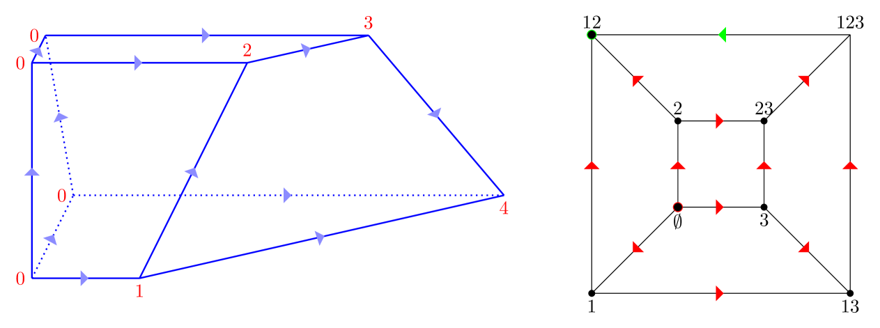
Figure 3: (Left) The (oriented) lopsided $3$-cube $\mathsf{Lop}_{3}$, its vertices labeled by their first coordinate. (Right) The graph of $\mathsf{Lop}_{3}$ directed by $(1,1,1)$, its vertices ${\boldsymbol{u}}_{X}$ labeled by $X$, its source and sink encircled in red and green, respectively. There are 2 paths of length 2, and 4 paths of length 4.

We now extend the previous construction to arbitrary dimension, using prisms.

Definition 4.2.

For a polytope $\mathsf{P}\subset\mathbb{R}^{d}$, its $k$-fold (standard) prism $\mathsf{Prism}_{k}\mathsf{P}$ is defined as follows: $\mathsf{Prim}_{k}\mathsf{P}\coloneqq\operatorname{conv}\Bigl{(}({\boldsymbol{v}},{\boldsymbol{e}}_{X})~;~{\boldsymbol{v}}\in\mathsf{P},~X\subseteq[k]\Bigr{)}\subset\mathbb{R}^{d+k}$, where ${\boldsymbol{e}}_{X}=\sum_{i\in X}{\boldsymbol{e}}_{i}\in\mathbb{R}^{k}$ for $X\subseteq[k]$.

For $d\geq 4$, the lopsided $d$-cube $\mathsf{Lop}_{d}$ is defined as the $(d-3)$-fold prism over $\mathsf{Lop}_{3}$. Explicitly, setting $X_{\leq d-3}=X\cap[d-3]$, $X_{\geq d-2}=\bigl{\{}i-d+3~;~i\in X\cap\{d-2,d-1,d\}\bigr{\}}$, and${\boldsymbol{u}}_{X}\coloneqq({\boldsymbol{u}}_{X_{\geq d-2}},{\boldsymbol{e}}_{X_{\leq d-3}})$ for $X\subseteq[d]$, the lopsided $d$-cube is $\mathsf{Lop}_{d}=\operatorname{conv}({\boldsymbol{u}}_{X}~;~X\subseteq[d])$.

In the following, we count (coherent) monotone paths on $\mathsf{Lop}_{d}$ for ${\boldsymbol{c}}=(1,\ldots,1)$. It is not hard to see that any ${\boldsymbol{c}}$-monotone path is coherent: iterating [10, Proposition 3.2.1], one obtains the following relation between coherent paths of a polytope and coherent paths of its $k$-fold prism.

Lemma 4.3.

For ${\boldsymbol{c}}\in\mathbb{R}^{d}$, the number of $({\boldsymbol{c}},1,\dots,1)$-monotone paths of length $k+\ell$ on $\mathsf{Prism}_{k}\mathsf{P}$ is $\frac{(k+\ell)!}{\ell!}N_{\ell}$, where $N_{\ell}$ is the number of ${\boldsymbol{c}}$-monotone paths of length $\ell$ on $\mathsf{P}$.

Proof.

We give a self-contained proof: the idea is similar to applying [10, Prop. 3.2.1] $k$ times.

Recall that a permutation $\sigma\in{\mathcal{S}}_{i+j}$ is a shuffle between $\sigma_{1}\in{\mathcal{S}}_{i}$ and $\sigma_{2}\in{\mathcal{S}}_{j}$ if $\sigma\left|{}_{[1,i]}\right.=\sigma_{1}$ and $\sigma\left|{}_{[i+1,i+j]}\right.=\sigma_{2}$. For fixed $\sigma_{1}\in{\mathcal{S}}_{i}$ and $\sigma_{2}\in{\mathcal{S}}_{j}$, there are $\binom{i+j}{i}$ shuffles between $\sigma_{1}$ and $\sigma_{2}$.

For this proof, we see a monotone path as an ordered list (i.e., a permutation) of (oriented) edges. Consider a $({\boldsymbol{c}},1,\dots,1)$-monotone path ${\mathcal{L}}$ of length $k+\ell$ on $\mathsf{Prism}_{k}\mathsf{P}$. There are two kind of (oriented) edges in ${\mathcal{L}}$: edges parallel to an edge of $\mathsf{P}$ (oriented according to ${\boldsymbol{c}}$), and edges parallel to ${\boldsymbol{e}}_{i}$ for some $i\in[d+1,d+k]$. There are necessarily $k$ edges of the second kind, hence there are $\ell$ edges of the first kind. Thus, ${\mathcal{L}}$ is a shuffle between a ${\boldsymbol{c}}$-monotone path of length $\ell$ on $\mathsf{P}$, and a path in the cube $\square_{k}$. Reciprocally, any shuffle between a ${\boldsymbol{c}}$-monotone path of length $\ell$ on $\mathsf{P}$ and a path in the cube $\square_{k}$ gives rise to a $({\boldsymbol{c}},1,\dots,1)$-monotone path on $\mathsf{Prism}_{k}\mathsf{P}$.

The number of such shuffle is $\binom{k+\ell}{\ell}\,N_{\ell}\,k!=\frac{(k+\ell)!}{\ell!}N_{\ell}$. ∎

Example 4.4.

The lopsided cube $\mathsf{Lop}_{d}$ is combinatorially isomorphic to $[0,1]^{d}$, and for ${\boldsymbol{c}}=(1,\dots,1)$ its graph, directed along ${\boldsymbol{c}}$, differs from the one of the standard cube $[0,1]^{d}$, just by reversing the edges ${\boldsymbol{u}}_{X}\to{\boldsymbol{u}}_{Y}$ for which $X_{\geq d-2}=\{1,2\}$ and $Y_{\geq d-2}=\{1,2,3\}$. The minimum and maximum vertex for this orientation is ${\boldsymbol{v}}_{\min}={\boldsymbol{u}}_{\varnothing}=(0,\dots,0)$ and ${\boldsymbol{v}}_{\max}={\boldsymbol{u}}_{[d-1]}=(4,1,0,1,\dots,1)$, respectively. Applying Lemma˜4.3 to Example˜4.1 yields that the number of (coherent) monotone paths on $\mathsf{Lop}_{d}$, counted by length, is given by the following non-unimodal sequence:

$\ell$	$d-1$	$d$	$d+1$	total
$N_{\ell}=N^{\text{coh}}_{\ell}$	$(d-1)!$	$0$	$\frac{1}{6}(d+1)!$	$(d-1)!\left(1+\frac{d(d+1)}{6}\right)$

This counterexample proves the following theorem, which makes ˜B (1) more explicit.

Theorem 4.5.

For all $d\geq 3$, there exist a $d$-dimensional polytope $\mathsf{P}\subset\mathbb{R}^{d}$, combinatorially isomorphic to a $d$-cube, and a direction ${\boldsymbol{c}}\in\mathbb{R}^{d}$, such that the sequences, $(N_{\ell})_{\ell}$ and $(N_{\ell}^{\text{coh}})_{\ell}$ of the number ${\boldsymbol{c}}$-monotone paths and of coherent paths, counted according to length, are not unimodal.

Remark 4.6.

It may seem quite underwhelming to use an abundance of $0$s to construct a non-unimodal sequence. Without digging ourselves in the quagmire of technicalities, we will now showcase a general method to address this issue, and provide one explicit example.

The idea is to start from the lopsided $d$-cube, and to perform a vertex truncation at its maximal vertex, i.e., to intersect $\mathsf{Lop}_{d}$ with a half-space $H_{{\boldsymbol{a}},b}^{-}=\{{\boldsymbol{x}}\in\mathbb{R}^{d}~;~\left<{\boldsymbol{x}},{\boldsymbol{a}}\right>\leq b\}$ that contains all vertices of $\mathsf{Lop}_{d}$ except ${\boldsymbol{u}}_{[d-1]}$. We set $\mathsf{P}_{{\boldsymbol{a}},b}=\mathsf{Lop}_{d}\cap H_{{\boldsymbol{a}},b}^{-}$. If ${\boldsymbol{a}}$ is linearly independent from $(1,\dots,1)$, then $(1,\dots,1)$ is generic for $\mathsf{P}_{{\boldsymbol{a}},b}$. As $\mathsf{Lop}_{d}$ is a simple polytope, $G_{\mathsf{P}_{{\boldsymbol{a}},b},(1,\dots,1)}$ is obtained from $G_{\mathsf{Lop}_{d},(1,\dots,1)}$ by replacing the vertex ${\boldsymbol{u}}_{[d-1]}$ by an oriented clique on its adjacent edges. Such a graph is likely to exhibit a non-unimodal number of monotone paths per length.

For $d=3$, we need to modify $\mathsf{Lop}_{3}$: we draw in Figure˜4 (Right) a $3$-dimensional simple polytope with $(N_{\ell})_{2\leq\ell\leq 5}=(1,{\color[rgb]{1,0,0}2},{\color[rgb]{1,0,0}1},{\color[rgb]{1,0,0}3})$, obtained from $\mathsf{Lop}_{3}$ by moving one vertex and truncating another. For $d=4$, taking e.g., ${\boldsymbol{a}}=(2,4,3,3)$, $b=20.5$ produces $\mathsf{P}_{{\boldsymbol{a}},b}$ with $(N_{\ell})_{4\leq\ell\leq 8}=(6,{\color[rgb]{1,0,0}22},{\color[rgb]{1,0,0}6},{\color[rgb]{1,0,0}8},4)$. We do not give a general formula for all dimensions, but random computer experiments tend to show that this method provides non-unimodal sequences with no internal $0$s.

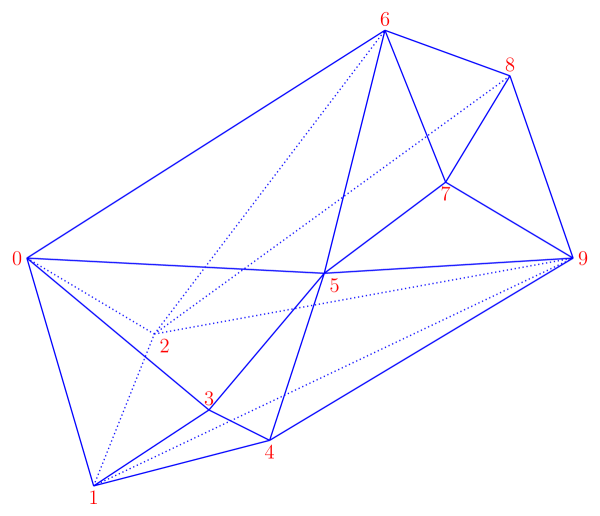
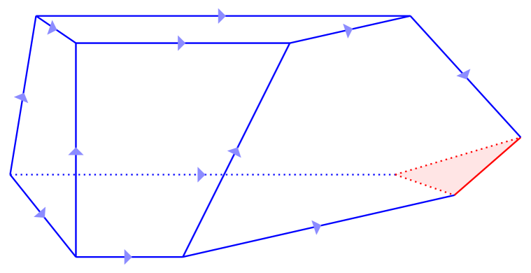
Figure 4: (Left) The $3$-dimensional simplicial polytope $\mathsf{P}_{10}$ from Example˜4.8. (Right) The $3$-dimensional simple polytope from Example˜4.4

4.2 Simplicial polytopes

Up to now, the examples providing a negative answer to ˜A were exclusively simple polytopes. One might wonder what happens for simplicial polytopes. Due to the fact that for a$d$-simplex, $N_{\ell}=\binom{d-1}{\ell-1}$ is the epitome of unimodal sequences (symmetric and ultra-log-concave), one might hope that ˜A has a positive answer for simplicial polytopes. We show this is false by providing an example. We prove in the next example, this refinement of ˜B (2):

Theorem 4.7.

There exists a $3$-dimensional polytope $\mathsf{P}\subset\mathbb{R}^{3}$ with $10$ vertices, such that the sequence $(N_{\ell})_{\ell}$ of the number of monotone paths of length $\ell$ on $\mathsf{P}$ for ${\boldsymbol{c}}=(1,0,0)$ is not unimodal.

Example 4.8.

Let $\mathsf{P}_{10}\subset\mathbb{R}^{3}$ be the polytope defined as the convex hull of the following $10$ vertices: $(0,0,0),(1,-5,-5),(2,0,-5),(3,-5,0),(4,-6,0),(5,-3,5),(6,5,5),(7,0,5),(8,5,2),(9,0,0)$.

$\mathsf{P}_{10}$ is depicted in Figure˜4 (Left), its vertices ${\boldsymbol{v}}$ being labeled by $\left<{\boldsymbol{v}},{\boldsymbol{e}}_{1}\right>$. We count monotone paths on $\mathsf{P}_{10}$ with respect to the direction ${\boldsymbol{c}}=(1,0,0)$ (from $(0,0,0)$ to $(9,0,0)$). It is easy to verify that one gets the following non-unimodal sequence.

$\ell$	2	3	4	5	6	7	8	total
$N_{\ell}$	3	8	12	11	12	6	1	53

Remark 4.9.

Let ${\boldsymbol{b}}$ be the barycenter of $\mathsf{P}_{10}$. One can embed the vertices of $\mathsf{P}_{10}$ on the 2-dimensional sphere $\mathbb{S}^{2}=\{{\boldsymbol{x}}\in\mathbb{R}^{3}~;~\|{\boldsymbol{x}}\|=1\}$ via the map ${\boldsymbol{x}}\mapsto\frac{{\boldsymbol{x}}-{\boldsymbol{b}}}{\|{\boldsymbol{x}}-{\boldsymbol{b}}\|}$. Let $\overline{\mathsf{P}}_{10}$ be the resulting polytope, defined as the convex hull of the images of the vertices of $\mathsf{P}_{10}$. This polytope is also simplicial but the graph of $\overline{\mathsf{P}}_{10}$, directed according to ${\boldsymbol{e}}_{1}$ differs from the corresponding directed graph of $\mathsf{P}_{10}$. One can verify that its numbers of ${\boldsymbol{e}}_{1}$-monotone paths on $\overline{\mathsf{P}}_{10}$ counted by length is given by the non-unimodal sequence $(4,8,{\color[rgb]{1,0,0}10},{\color[rgb]{1,0,0}8},{\color[rgb]{1,0,0}11},6,1)$, the shortest path having 2 edges.

As slightly modifying the coordinates of the vertices of $\overline{\mathsf{P}}_{10}$ does not change its directed graph, there exists a subset ${\mathcal{A}}\subseteq(\mathbb{S}^{2})^{10}$, which is not of measure $0$, such that if ${\boldsymbol{x}}_{1},\dots,{\boldsymbol{x}}_{10}\in{\mathcal{A}}$, the number of ${\boldsymbol{e}}_{1}$-monotone paths of $\operatorname{conv}({\boldsymbol{x}}_{1},\dots,{\boldsymbol{x}}_{10})$ is non-unimodal. Said differently, constructing a polytope as the convex hull of $10$ points chosen uniformly at random on $\mathbb{S}^{2}$, there is a strictly positive probability that number of ${\boldsymbol{e}}_{1}$-monotone path counted by length is not unimodal (i.e., that the answer to ˜A is “no”). The reader should keep this in mind while reading Section˜5.

Problem 4.10.

Find a simplicial polytope whose number of coherent paths counted according to length $(N^{\text{coh}}_{\ell})_{\ell}$ is not unimodal (we found a non-log-concave example, but do not present it here).

4.3 Loday’s associahedron of dimension 5

For $n\geq 3$, Loday’s $n$-associahedron $\mathsf{Asso}_{n}\subset\mathbb{R}^{n}$ is a $(n-1)$-dimensional generalized permutahedron (i.e., its edge directions are ${\boldsymbol{e}}_{i}-{\boldsymbol{e}}_{j}$ for some $1\leq i<j\leq n$) having the following facet-description:

$$\mathsf{Asso}_{n}=\left\{{\boldsymbol{x}}\in\mathbb{R}^{n}~;~\begin{array}[]{l}\sum_{i=1}^{n}x_{i}=0\\ \sum_{i\in I}x_{i}\geq\binom{|I|+1}{2}~~\text{ for }~~\varnothing\neq I=[a,b]\subsetneq[n]\end{array}\right\}$$

It is known that the graph of $\mathsf{Asso}_{n}$, directed by ${\boldsymbol{c}}=(1,2,\dots,n)$, is the Hasse diagram of the Tamari lattice. For a detailed description of Loday’s associahedron and its deep links with the Tamari lattice, we refer the interested reader to [26, 32]. The number $N_{\ell}$ of monotone paths on Loday’s associahedron $\mathsf{Asso}_{n}$ for ${\boldsymbol{c}}=(1,2,\dots,n)$ hence coincides with the number of maximal chains in the Tamari lattice. The latter was computed by Nelson [30, Thm. 5.9], and discussed in the general context of graph associahedra by Dahlberg & Fishel [19]. Nelson gives the following sequence $N_{\ell}$ for $n=6$, see also OEIS A282698, which we completed by computing $N^{\text{coh}}_{\ell}$ ($\ell$ is the number of edges in the path, so there is an offset with respect to Nelson’s notation):

Source	$\ell$	6	7	8	9	10	11	12	13	14	15	16	total
[30], A282698	$N_{\ell}$	1	20	112	232	382	348	456	390	420	334	286	2981
Our computation	$N^{\text{coh}}_{\ell}$	1	20	105	206	332	274	332	270	206	122	142	2010

Both sequences are not unimodal, as the highlighted sub-sequences in red show. To obtain the above sequence $N^{\text{coh}}_{\ell}$, we used two methods described in Section˜6 (we also confirmed OEIS A282698 up to $n=6$). This example proves the following theorem (see ˜B (3)):

Theorem 4.11.

There exist a $5$-dimensional generalized permutahedron $\mathsf{P}$ and a direction ${\boldsymbol{c}}\in\mathbb{R}^{6}$ such that the sequences $(N_{\ell})_{\ell}$ and $(N_{\ell}^{\text{coh}})_{\ell}$ of the number of ${\boldsymbol{c}}$-monotone paths and coherent paths of length $\ell$ on $\mathsf{P}$ are not unimodal.

Remark 4.12.

Using the methods, described in Section˜6, one gets the following sequences for $N_{\ell}$ and $N_{\ell}^{\text{coh}}$ for the $4$-dimensional polytope $\mathsf{Asso}_{5}$ with respect to $c=(1,2,3,4,5)$ (see also [30]):

Source	$\ell$	4	5	6	7	8	9	10	total
[30], A282698	$N_{\ell}$	1	10	22	22	18	13	12	98
Our computation	$N^{\text{coh}}_{\ell}$	1	10	21	21	18	9	10	90

As can be seen from the table, the sequence $(N_{\ell})_{\ell}$ is unimodal while the sequence $(N_{\ell})^{\text{coh}}$ is not.

Besides, for $n=7$, the sequence $(N^{\text{coh}}_{\ell})_{\ell}$ has several non-unimodal sub-triples; but for $n=8$, the sequence $(N^{\text{coh}}_{\ell})_{\ell}$ is unimodal.

In general, counting coherent paths on Loday’s associahedron is open, to our knowledge (and seems difficult). Nelson interprets maximal chains in the Tamari lattice (i.e., monotone paths on Loday’s associahedron) as tableaux, however note that that the notion of coherence of a path is not equivalent to the realizability of Young tableaux developed in [29, 1] (see also [16, Section 8] for a more general perspective in the context of coherent paths on the permutahedron).

Problem 4.13.

Describe and count the coherent paths on Loday’s associahedron for ${\boldsymbol{c}}=(1,2,\dots,n)$.

4.4 Polytopes with 0/1-coordinates

Some readers may argue that the counterexamples we showed, though of a significant theoretical importance, are a bit too “wild” to discourage people from believing that the sequences $(N_{\ell})_{\ell}$ and $(N^{\text{coh}}_{\ell})_{\ell}$ are unimodal. Even though the counterexamples from the previous subsection were for “nice classes” of polytopes (simple, simplicial, 3-dimensional polytopes, polytopes with few edge directions), these examples had in common that we used “big” coordinates in order to construct quite convoluted behaviors of paths. In this section, we tackle this belief by presenting a counterexample with $0/1$-coordinates. In particular, we make ˜B (4) more explicit.

A polytope $\mathsf{P}\subset\mathbb{R}^{n}$ is a $0/1$-polytope if ${\boldsymbol{v}}\in\{0,1\}^{n}$ for each vertex ${\boldsymbol{v}}$ of $\mathsf{P}$, i.e., all its vertices are vertices of the $n$-cube $[0,1]^{n}$. As every such vertex is determined by its set of coordinates equal to $1$, we associate to any set ${\mathcal{X}}$ of subsets $X\subseteq[n]$, a $0/1$-polytope $\mathsf{P}_{{\mathcal{X}}}$ in a natural way; namely:

$$\mathsf{P}_{{\mathcal{X}}}=\operatorname{conv}\left({\boldsymbol{e}}_{X}~;~X\in{\mathcal{X}}\right),$$

where ${\boldsymbol{e}}_{X}\coloneqq\sum_{i\in X}{\boldsymbol{e}}_{i}$. Thus, $0/1$-polytopes are in bijection with collections of subsets of $[n]$.

A common way to orient the graph $\mathsf{P}_{{\mathcal{X}}}$ is to use the direction ${\boldsymbol{c}}_{\text{lex}}=(2^{1},2^{2},\dots,2^{n})\in\mathbb{R}^{n}$. The orientation that ${\boldsymbol{c}}_{\text{lex}}$ induces on the graph of $\mathsf{P}_{{\mathcal{X}}}$ is given by the (reverse) lexicographic order: if $[{\boldsymbol{e}}_{X},{\boldsymbol{e}}_{Y}]$ is an edge of $\mathsf{P}_{{\mathcal{X}}}$, then $\left<{\boldsymbol{e}}_{X},{\boldsymbol{c}}_{\text{lex}}\right><\left<{\boldsymbol{e}}_{Y},{\boldsymbol{c}}_{\text{lex}}\right>$ if and only if $X=\{x_{r}>\dots>x_{1}\}$ is lexicographically smaller than $Y=\{y_{s}>\dots>y_{1}\}$. We found several $0/1$-polytopes whose the sequence $(N_{\ell})_{\ell}$ of the number of ${\boldsymbol{c}}_{\text{lex}}$-monotone paths of length $\ell$ is not unimodal. We present one.

Example 4.14.

To simplify notations, we use $123$ to denote $\{1,2,3\}$ and similarly for other subsets. Let ${\mathcal{X}}$ be the collection of all subsets of $[5]$ contained in $14$, $1235$ or $2345$ (equivalently, ${\mathcal{X}}$ is the simplicial complex with facets $14$, $1235$ and $2345$). The polytope $\mathsf{P}_{{\mathcal{X}}}\subset\mathbb{R}^{5}$ is neither simple nor simplicial and its $f$-vector is $(1,25,75,90,51,13,1)$. For the direction ${\boldsymbol{c}}_{\text{lex}}=(2^{1},2^{2},2^{3},2^{4},2^{5})$, the sequence $(N_{\ell})_{\ell}$ of the number of ${\boldsymbol{c}}_{\text{lex}}$-monotone paths on $\mathsf{P}_{{\mathcal{X}}}$ is the following:

$\ell$	3	4	5	6	7	8	total
$N_{\ell}$	2	36	96	76	84	36	330

As the highlighted sub-sequence in red shows, this sequence is not unimodal.

This example proves the following statement:

Theorem 4.15.

There exists a $5$-dimensional $0/1$-polytope $\mathsf{P}\subset\mathbb{R}^{5}$ with $25$ vertices such that, for ${\boldsymbol{c}}_{\text{lex}}=(2^{1},2^{2},2^{3},2^{4},2^{5})$, the sequence $(N_{\ell})_{\ell}$ of the number of ${\boldsymbol{c}}_{\text{lex}}$-monotone paths of length $\ell$ on $\mathsf{P}$ is not unimodal.

Remark 4.16.

According to our computations, besides the simplicial complex in Example˜4.14, there are only two other simplicial complexes on $5$ vertices or less, such that the sequences of the number of ${\boldsymbol{c}}_{\text{lex}}$-monotone paths of length $\ell$ are not unimodal: Namely, the one with facets $24$, $1235$ and $1345$, and the one with facets $3$ and $1245$. We want to emphasize, that these are all such counterexamples and not just counterexamples up to symmetry, since orienting by ${\boldsymbol{c}}_{\text{lex}}$ breaks any symmetry. We also found several counterexamples on 6 vertices.

All counterexamples we found turned out to come from non-pure simplicial complexes (some of them not even connected). Though we were not able to found a pure simplicial complex, giving rise to a counterexample, we conjecture that such pure simplicial complexes exist but are just too big to be found by an exhaustive search through all pure simplicial complexes. This conjecture is supported the fact that for $(\mathsf{P}_{{\mathcal{X}}},{\boldsymbol{c}}_{\text{lex}})$ with ${\mathcal{X}}$ the pure simplicial complex with facets $123$, $134$, $245$ and $345$, the sequence $(N_{\ell})_{\ell\geq 3}=(8,40,67,62,22,8)$ is easily seen to be not log-concave.

Coherent paths

With an exhaustive computer search, we can certify that for any $4$-dimensional $0/1$-polytope $\mathsf{P}\subset\mathbb{R}^{4}$, and for any $5$-dimensional $0/1$-polytope of the form $\mathsf{P}_{{\mathcal{X}}}$, where ${\mathcal{X}}$ is a simplicial complex on $5$ vertices, the sequence $(N^{\text{coh}}_{\ell})_{\ell}$ of the number of coherent paths in direction ${\boldsymbol{c}}_{\text{lex}}=(2^{1},\dots,2^{n})$ of length $\ell$ is unimodal. For simplicial complexes on $[5]$, they are log-concave.

However, we conjecture this to be false in higher dimensions (or already in dimension $5$ if the polytope is not coming from a simplicial complex). We found a $4$-dimensional $0/1$-polytope $\mathsf{P}_{{\mathcal{X}}}$ whose number of coherent paths per length, in direction ${\boldsymbol{c}}_{\text{lex}}=(2^{1},2^{2},2^{3},2^{4})$, is not log-concave. Namely, for ${\mathcal{X}}=\{\varnothing,1,2,12,13,34,124\}$, the sequence $(N^{\text{coh}}_{\ell})_{\ell\geq 2}=(1,4,4,5,2)$ is not log-concave.

Problem 4.17.

Find a $0/1$-polytope, coming from a (pure) simplicial complex, whose number of coherent paths counted by length $(N^{\text{coh}}_{\ell})_{\ell}$ is not a unimodal sequence, for the direction ${\boldsymbol{c}}_{\text{lex}}$.

Note that linear optimization on $0/1$-polytopes has been largely studied, see [11] and its section “Prior work and context”. There are polynomial algorithms for finding short paths, hence the above problem is more of theoretical importance, rather than practical one.

5 Random case

We have seen that, even for sufficiently nice classes of polytopes, including simple and simplicial polytopes, as well as generalized permutahedra and $0/1$-polytopes, ˜A has a negative answer in general. However, all counterexamples we gave were rather special in the way we constructed them. Moreover, experimenting with at random polytopes with vertices on the sphere, it seems rather hard to find an example of a polytope that contradicts ˜A (see Remark˜4.9). In the following, we make this intuition precise. While, morally, the question of monotone paths is a problem in dimension $d$, understanding coherent paths amounts to studying 2-dimensional projections of a $d$-dimensional polytope. Since the latter seems to be more tractable, we will focus on coherent paths. We start by formulating our main result (˜B from the introduction).

Theorem 5.1.

Fix (deterministically or at random) linearly independent vectors ${\boldsymbol{c}},{\boldsymbol{\omega}}\in\mathbb{R}^{d}$.Let $Z_{1},\dots,Z_{n}$ be points taken uniformly at random, independently, on the sphere $\mathbb{S}^{d-1}\subset\mathbb{R}^{d}$, and $\mathsf{P}_{n}=\operatorname{conv}(Z_{1},\dots,Z_{n})$. Then, the length $L_{n}$ of the coherent ${\boldsymbol{c}}$-monotone path captured by ${\boldsymbol{\omega}}$ on $\mathsf{P}_{n}$ admits a central limit theorem, i.e.,

$$\frac{L_{n}-\mathbb{E}(L_{n})}{\sqrt{\operatorname{Var}(L_{n})}}\xrightarrow[n\to+\infty]{}U~~~~\text{ (convergence is in distribution)},$$

with $U\sim{\mathcal{N}}(0,1)$ a standard normally distributed random variable with expectation $0$, variance $1$. Moreover, $\mathbb{E}(L_{n})\sim c\,n^{\frac{1}{d-1}}$ for some $c>0$, and: $c^{\prime}\,n^{\frac{1}{d-1}-a}\leq\operatorname{Var}(L_{n})\leq c^{\prime\prime}\,(\log n)^{3-\frac{1}{d-1}}\,n^{\frac{1}{d-1}}$ for any $a>0$ and for some $c^{\prime},c^{\prime\prime}>0$.

We postpone the proof of this theorem to Section˜5, where it will follow from combining Corollaries˜5.5, 5.8, 5.17, 5.28 and 5.37.

This section might seem long and technical at first, especially for readers coming from a combinatorial or polytopal background. However, the methods, though probabilistic by nature, use a lot of combinatorial and geometric arguments and ideas, and the reader might find them helpful for similar problems as they can be applied in rather general contexts. Indeed, these methods can be considered standard methods in the theory of random convex bodies/polytopes and have found multiple applications, see [27, Section 6], and also [36, 37, 14].

As our background also lies in combinatorics and polytope theory, we tried our best to not scare the reader, to keep this section as readable as possible, and to build a narrative from which the reader may extract useful information (methods, lemmas, ideas, citable results, etc.), adorned with meaningful illustrations. To this end, we have included a cheat sheet of formulas in Section˜5.3, and we strongly recommend to skip the detailed proof in Section˜5.2, in a first reading, and instead to focus on the the theorems, corollaries and lemmas (the proof can be read in a second reading, for instance). Section˜5.1 explains the probabilistic model at stake by detailing the interaction between coherent paths (i.e., projections to $\mathbb{R}^{2}$) and the uniform distribution on the sphere $\mathbb{S}^{d-1}$. Section˜5.2 proves Theorem˜5.1 by analyzing the behavior of $\beta$-polygons in the plane, for $\beta>0$.

5.1 The probabilistic model

Let $Z_{1},\dots,Z_{n}$ be independently uniformly distributed points on the $(d-1)$-dimensional sphere $\mathbb{S}^{d-1}=\{x\in\mathbb{R}^{d}~;~\|x\|=1\}$, and let $\mathsf{P}_{n}=\operatorname{conv}(Z_{1},\dots,Z_{n})$ be the induced random polytope. Let ${\boldsymbol{c}}\in\mathbb{R}^{d}$ be a fixed direction. By rotational symmetry, we assume that ${\boldsymbol{c}}={\boldsymbol{e}}_{1}$. We are interested in the number $N_{\ell}^{\text{coh}}$ of coherent ${\boldsymbol{c}}$-monotone paths of length $\ell$ on $\mathsf{P}_{n}$, i.e., the histogram of the random variable giving length. Hence, to advocate that the sequence $(N^{\text{coh}}_{\ell})_{\ell}$ is “statistically unimodal”, we estimate its histogram by the probability distribution of this length.

For this, we let $L({\boldsymbol{\omega}},\mathsf{P}_{n})$ denote the random variable giving the length of the coherent monotone path on $\mathsf{P}_{n}$ captured by ${\boldsymbol{\omega}}$, where ${\boldsymbol{\omega}}\in\mathbb{S}^{d-1}$. By Definition˜2.3, $L({\boldsymbol{\omega}},\mathsf{P}_{n})$ is the length, i.e., the number of edges, of the upper path of the polygon obtained by projecting $\mathsf{P}_{n}$ onto the plane spanned by ${\boldsymbol{c}}$ and ${\boldsymbol{\omega}}$. We aim at understanding the distribution of $L({\boldsymbol{\omega}},\mathsf{P}_{n})$ for large $n$. In the following, we denote by $\pi_{{\boldsymbol{c}},{\boldsymbol{\omega}}}$ the orthogonal projection from $\mathbb{R}^{d}$ to the plane spanned by ${\boldsymbol{c}}$ and ${\boldsymbol{\omega}}$, see Figure˜6 (Left). The next lemma, which is a special case of [25], shows that the random variables $\pi_{{\boldsymbol{c}},{\boldsymbol{\omega}}}(Z_{1}),\dots,\pi_{{\boldsymbol{c}},{\boldsymbol{\omega}}}(Z_{n})$ follow a ($2$-dimensional) $\beta$-distribution (for a specific value $\beta$).

Lemma 5.2 (Adapted from [25, Lemma 4.3 (a)]).

Let ${\boldsymbol{E}}$ be a $2$-dimensional plane in $\mathbb{R}^{d}$ and let $\pi_{{\boldsymbol{E}}}:\mathbb{R}^{d}\to{\boldsymbol{E}}$ be the orthogonal projection onto ${\boldsymbol{E}}$. If a random variable $Z$ is distributed according to the uniform distribution on the sphere $\mathbb{S}^{d-1}$, then the projected random variable $\pi_{{\boldsymbol{E}}}(Z)$ is distributed according to the probability density (where $\beta_{d}=\frac{d}{2}-2$ and $C_{2,\beta_{d}}=\frac{1}{\pi}\frac{\Gamma(\beta_{d}+2)}{\Gamma(\beta_{d}+1)}$):

$$f_{2,\beta_{d}}({\boldsymbol{x}})=C_{2,\beta_{d}}\,\left(1-\|{\boldsymbol{x}}\|^{2}\right)^{\beta_{d}}~~~\text{ for }{\boldsymbol{x}}\in\mathbb{B}^{2},$$

Example 5.3.

For $d=3$, we have $\beta_{3}=-\frac{1}{2}$ and the density $f_{2,\beta_{3}}({\boldsymbol{x}})$ gets higher the closer a point ${\boldsymbol{x}}$ is to the boundary of the disk $\mathbb{B}^{2}=\{x\in\mathbb{R}^{2}~;~\|x\|=1\}$, see Figure˜5 (Left).

For $d=4$, we have $\beta_{4}=0$: the $2$-dimensional $\beta_{4}$-distribution is the uniform distribution on $\mathbb{B}^{2}$. Reitzner [34] proved that, for the convex hull of $n$ uniformly distributed independent random points in a convex set (in any dimension), the numbers of $k$-faces satisfy a central limit theorem.

For $d\geq 5$, we have $\beta_{d}>0$, and the density $f_{2,\beta_{d}}({\boldsymbol{x}})$ gets lower the closer a point ${\boldsymbol{x}}$ is to the boundary of $\mathbb{B}^{2}$. In particular, the higher the dimension, the more the distribution is concentrated around the center of the disk, and the sparser it gets towards the boundary, see Figures˜5 and 6.

Due to this different behavior, of the density for $d\leq 3$ and $d\geq 4$, in the following, we will only consider the case that $d\geq 4$.

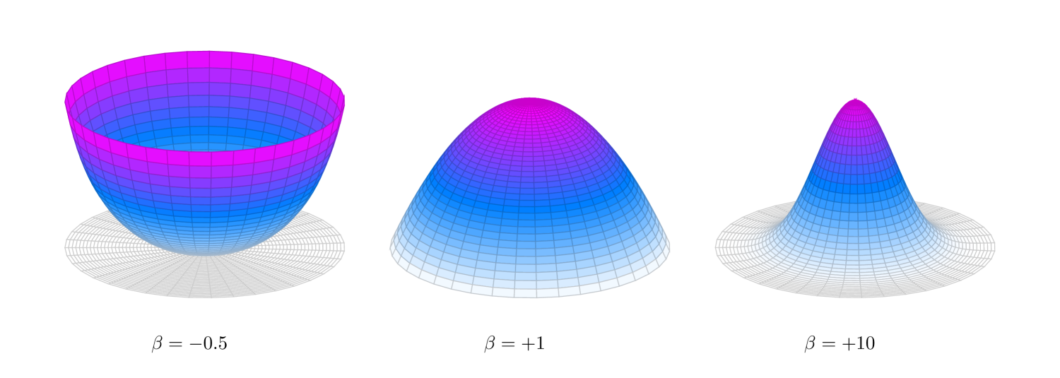
Figure 5: Examples of $\beta$-distributions, for $\beta\in\{-\frac{1}{2},+1,+10\}$, or equivalently $d\in\{3,6,22\}$. A negative $\beta$ implies that the probability density goes to $+\infty$ on $\mathbb{S}^{1}$, whereas a positive $\beta$ implies it goes to $0$ on $\mathbb{S}^{1}$. The bigger $\beta$ the more the distribution is concentrated around the center of $\mathbb{B}^{2}$.

By Lemma˜5.2, the projected points $X_{i}\coloneqq\pi_{{\boldsymbol{c}},{\boldsymbol{\omega}}}(Z_{i})$ are independently identically distributed (i.i.d. for short) with probability density function $f_{2,\frac{d}{2}-2}$. The next definition is essential:

Definition 5.4.

For $X_{1},\dots,X_{n}$ independently identically $\beta$-distributed random points on the disk $\mathbb{B}^{2}$ with $\beta=\frac{d}{2}-2$, we set $\mathsf{Q}_{n}=\operatorname{conv}(X_{1},\dots,X_{n})$.

We use $f_{1}^{\text{up}}(\mathsf{Q}_{n})$ to denote the number of edges of the upper path of $\mathsf{Q}_{n}$, i.e., $f_{1}^{\text{up}}(\mathsf{Q}_{n})$ counts the number of edges of $\mathsf{Q}_{n}$ whose outer normal vector has a positive second coordinate (see Section˜2). We denote $f_{1}^{\text{low}}(\mathsf{Q}_{n})$ the number of edges of the lower path. By Definition˜2.3, $L({\boldsymbol{\omega}},\mathsf{P}_{n})=f_{1}^{\text{up}}(\mathsf{Q}_{n})$, for $\mathsf{Q}_{n}=\pi_{{\boldsymbol{c}},{\boldsymbol{\omega}}}(\mathsf{P}_{n})$. By symmetry, $f_{1}^{\text{low}}$ and $f_{1}^{\text{up}}$ are identically distributed, but not independent! Hence, one can show that, after normalization, they converge to a normal distribution if and only if $f_{1}(\mathsf{Q}_{n})$ $=f_{1}^{\text{up}}(\mathsf{Q}_{n})+f_{1}^{\text{low}}(\mathsf{Q}_{n})$ satisfies a central limit theorem (see Section˜5 for the details). As $\mathsf{Q}_{n}$ is a polygon, its number of vertices $f_{0}(\mathsf{Q}_{n})$ satisfy $f_{0}(\mathsf{Q}_{n})=f_{1}(\mathsf{Q}_{n})$. We hence need to show that $f_{0}(\mathsf{Q}_{n})$ obeys a central limit theorem. We summarize this discussion in the next corollary:

Corollary 5.5.

Let ${\boldsymbol{c}},{\boldsymbol{\omega}}\in\mathbb{S}^{d-1}$, and let $\mathsf{P}_{n}=\operatorname{conv}(Z_{1},\dots,Z_{n})$, where $Z_{1},\dots,Z_{n}$ are i.i.d. points on $\mathbb{S}^{d-1}$. Let $\mathsf{Q}_{n}=\operatorname{conv}(X_{1},\dots,X_{n})$, where $X_{1},\dots,X_{n}$ are independently $\beta$-distributed with $\beta=\frac{d}{2}-2$. Then, the random variables $L({\boldsymbol{\omega}},\mathsf{P}_{n})$, $f_{1}^{\text{up}}(\mathsf{Q}_{n})$ and $f_{1}^{\text{low}}(\mathsf{Q}_{n})$ have the same distribution.

Proof.

By Lemma˜5.2, the random variables $L({\boldsymbol{\omega}},\mathsf{P}_{n})$ and $f_{1}^{\text{up}}(\mathsf{Q}_{n})$ are identically distributed. Moreover, due to rotational symmetry, $f_{1}^{\text{up}}(\mathsf{Q}_{n})$ and $f_{1}^{\text{low}}(\mathsf{Q}_{n})$ also have the same distribution. ∎

Example 5.6.

With a computer, we can sample $n$ points on a $(d-1)$-dimensional sphere, project them into dimension $2$ (by forgetting all but their first two coordinates), and construct the convex hull of the projected points. Varying $d$, and hence $\beta_{d}$, give rise to different pictures, see Figure˜6. Again, one observes that the points get more concentrated around the center, when $\beta$ grows.

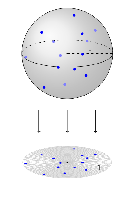
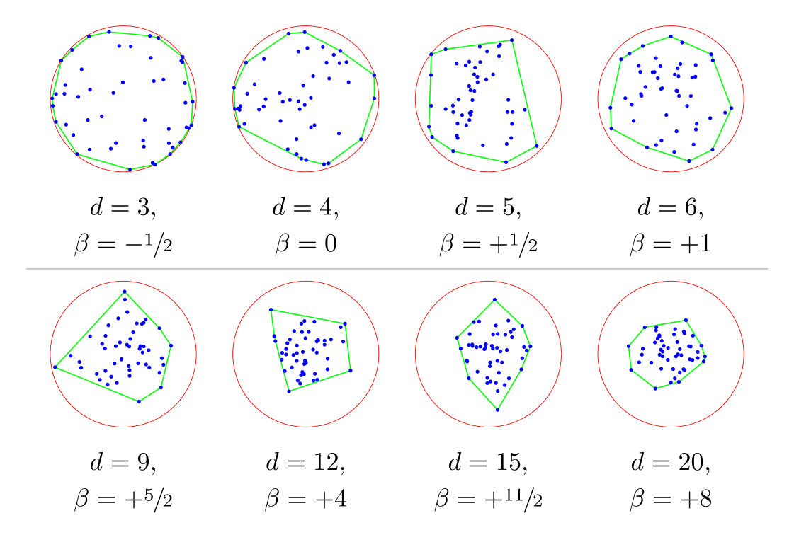
Figure 6: For each $d$, we sampled $n=50$ points uniformly at random on the $(d-1)$-sphere and projected them onto the disk $\mathbb{B}^{2}$. The convex hull $\mathsf{Q}_{n}$ of the projected points is shown in green.

As $f_{0}(\mathsf{Q}_{n})$ will be of prime importance for the remaining section, we can determine its mean value over several samples, see Figure˜7. This number seems to grow slowly towards $+\infty$. We will see in Corollary˜5.8 that the exact estimate for the expected value is proportional to $n^{\frac{1}{d-1}}$.

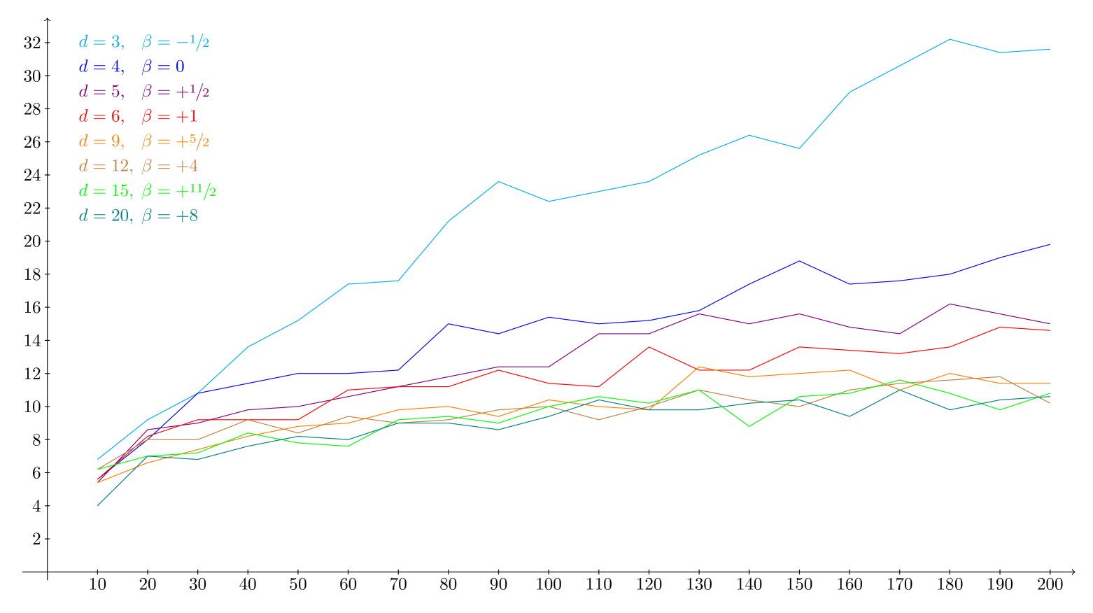
Figure 7: For each $\beta$, and for $n=10k$ with $k\in\{1,\dots,20\}$, we sample $n$ points according to the $\beta$-distribution, compute the convex hull and counts its number of edges/vertices. We show the mean value obtained by doing 5 of these samples for each $(\beta,n)$.

5.2 The number of vertices of $\beta$-polygons in the plane

In this section, for fix $d$, we consider the polygon $\mathsf{Q}_{n}$ obtained by picking $n$ i.i.d. random points on the sphere $\mathbb{S}^{d-1}$, and taking the convex hull of their orthogonal projections to the disk $\mathbb{B}^{2}$. This gives to $n$ points in the plane, distributed according to the density function $f_{2,\frac{d}{2}-2}$ (Section˜5.1).

Note that $\mathsf{Q}_{n}$ is a random variable. We will let $n$ tend towards $+\infty$ to determine the limiting behavior of properties of $\mathsf{Q}_{n}$: firstly, the asymptotics of the expected value and variance of $f_{0}(\mathsf{Q}_{n})$.

In what follows, a constant will refer to a positive non-zero number that only depends on the parameter $\beta$ or the dimension $d$, rather than anything else, as e.g., , the number of vertices $n$, a small value $\varepsilon$, a radius $R$. Apart from the constant $c_{0}$ defined in $\varepsilon=c_{0}\frac{\log n}{n}$ (see Section˜5.2.2 for the details), all other constants have no importance, and, slightly abusing notation, will simply be named $c$. In particular, this means that the exact value of $c$ might change from one line to the next: $c$ should be thought of as a symbol, not a real value.

In addition, if $\beta$ is clear from the context, we use $\mu(A)$ to denote the measure of a set $A\subseteq\mathbb{B}^{2}$ according to the probability density $f_{2,\beta}({\boldsymbol{x}})=C_{2,\beta}\,(1-\|{\boldsymbol{x}}\|^{2})^{\beta}$, see Section˜5.1. Throughout this section, we assume: $\beta=\frac{d}{2}-2$.

All limits, equivalents, approximations, etc., are done assuming $n\to+\infty$, $\varepsilon\to 0$, and $R\to 1$.

5.2.1 Expectancy

The expectancy of $f_{0}(\mathsf{Q}_{n})$ can be directly deduced from several papers on $\beta$-polytopes. Especially, we get the following from [25, Thm. 1.3, Rmk. 1.4]:

Theorem 5.7.

The expected number of facets for a $\beta$-distributed polytope obtained as the convex hull of $n$ points in dimension $D$ is:

$$\mathbb{E}\left(f_{D-1}(\mathsf{P}_{n,D}^{\beta})\right)=2\binom{n}{D}\,\int_{-1}^{+1}C_{1}\,(1-t^{2})^{\alpha_{1}}\left(\int_{-1}^{t}C_{2}\,(1-s^{2})^{\alpha_{2}}\,\mathrm{d}s\right)^{n-D}\,\mathrm{d}t$$

where $\alpha_{1}=D\beta+\frac{D^{2}-1}{2}$, $\alpha_{2}=\beta+\frac{D-1}{2}$, and $C_{1},C_{2}$ are real numbers with $\int_{-1}^{+1}C_{i}\,(1-x^{2})^{\alpha_{i}}\,\mathrm{d}x=1$.

Since, in dimension $2$, the number of facets equals its number of vertices, we can apply Theorem˜5.7 to $\mathsf{Q}_{n}$. Moreover, in this setting, we can determine the exact asymptotics of $\mathbb{E}(f_{0}(\mathsf{Q}_{n}))$:

Corollary 5.8.

Let $d\geq 5$. Then, the expected number of vertices of $\mathsf{Q}_{n}$ is:

$$\mathbb{E}\bigl{(}f_{0}(\mathsf{Q}_{n})\bigr{)}\sim c\,n^{\frac{1}{d-1}}$$

Proof.

The authors deeply thank Kinga Nagy, who helped calculate the integral.

Recall that $f_{0}(\mathsf{Q}_{n})=f_{1}(\mathsf{Q}_{n})$ as $\mathsf{Q}_{n}$ is a polygon. In the following, we apply Theorem˜5.7 with $D=2$ and $\beta=\frac{d}{2}-2$, and then estimate the asymptotics of the integral when $n\to+\infty$. We have

$$\mathbb{E}\bigl{(}f_{0}(\mathsf{Q}_{n})\bigr{)}=2\binom{n}{2}\int_{-1}^{+1}C_{1}(1-t^{2})^{\alpha_{1}}\left(\int_{-1}^{t}C_{2}(1-s^{2})^{\alpha_{2}}\,\mathrm{d}s\right)^{n-2}\,\mathrm{d}t,$$

where $\alpha_{1}=d-\frac{5}{2}$ and $\alpha_{2}=\frac{d}{2}-\frac{3}{2}$. Note that $\alpha_{i}>0$, since $d\geq 5$ (for $i=1,2$). First, $2\binom{n}{2}=n(n-1)\sim n^{2}$. Moreover, the integrals can be estimated as follows.

For $t\in\,]-1,+1[$, the integral $\int_{-1}^{t}(1-s^{2})^{\alpha_{2}}\,\mathrm{d}s$ is a number strictly between $0$ and $1$, which increases with $t$, and tends to $1$ if $t\to+1$. Hence, $\left(\int_{-1}^{t}(1-s^{2})^{\alpha_{2}}\,\mathrm{d}s\right)^{n-2}\to 0$, if $n\to+\infty$, and this convergence is at an exponential speed. To be precise, for fixed $y>0$, let $\rho_{y}=\int_{-1}^{1-y}(1-s^{2})^{\alpha_{2}}\,\mathrm{d}s$. Then, there is a constant $C>0$ such that:

$$\int_{-1}^{1-y}C_{1}(1-t^{2})^{\alpha_{1}}\left(\int_{-1}^{t}C_{2}(1-s^{2})^{\alpha_{2}}\,\mathrm{d}s\right)^{n-2}\,\mathrm{d}t~~\leq~~C\,\rho_{y}^{n}$$

On the other hand, changing for the variables $1-t$ and $1-s$, we get:

$$\int_{1-y}^{+1}C_{1}(1-t^{2})^{\alpha_{1}}\left(\int_{-1}^{t}C_{2}(1-s^{2})^{\alpha_{2}}\,\mathrm{d}s\right)^{n-2}\,\mathrm{d}t=\int_{0}^{y}C_{1}(2t-t^{2})^{\alpha_{1}}\left(1-\int_{0}^{t}C_{2}(2s-s^{2})^{\alpha_{2}}\,\mathrm{d}s\right)^{n-2}\,\mathrm{d}t$$

When $t\to 0$, we use $\frac{\partial\cdot}{\partial t}\int_{0}^{t}C_{2}(2s-s^{2})^{\alpha_{2}}\,\mathrm{d}s~=~C_{2}(2t-t^{2})^{\alpha_{2}}~=~C_{2}2^{\alpha_{2}}t^{\alpha_{2}}~~+O(t^{\alpha_{2}+1})$. Thus:

$$1-\int_{0}^{t}C_{2}(2s-s^{2})^{\alpha_{2}}\,\mathrm{d}s~=~1-\frac{C_{2}2^{\alpha_{2}}}{\alpha_{2}+1}t^{\alpha_{2}+1}~~+O(t^{\alpha_{2}+2})$$

Hence, we get the approximation:

$$\frac{1}{n^{2}}\mathbb{E}\bigl{(}f_{0}(\mathsf{Q}_{n})\bigr{)}=~C\rho_{y}^{n}~+~\int_{0}^{y}c_{1}2^{\alpha_{1}}t^{\alpha_{1}}\left(1-\frac{C_{2}2^{\alpha_{2}}}{\alpha_{2}+1}t^{\alpha_{2}+1}\right)^{n-2}\,\mathrm{d}t~~+O\left(y^{(n-2)(\alpha_{2}+2)+1}\right)$$

According to [8, formula 11], the last remaining integral is asymptotically $C^{\prime}\left(\frac{1}{n}\right)^{\frac{\alpha_{1}+1}{\alpha_{2}+1}}$ for some constant $C^{\prime}$ (precisely: there exists a sequence $(y_{n})_{n}$, converging to 0, such that the middle integral has this asymptotics and the other terms are negligible against it, when $n\to+\infty$). Using $\frac{\alpha_{1}+1}{\alpha_{2}+1}=\frac{2d-3}{d-1}=2-\frac{1}{d-1}$, this gives the claimed formula. ∎

Remark 5.9.

In his famous book [12], Borgwardt showed that Corollary˜5.8 also holds in the dual case. More precisely, for ${\boldsymbol{a}}_{1},\dots,{\boldsymbol{a}}_{m}\in\mathbb{R}^{d}$ are i.i.d. random vectors taken uniformly on the sphere, he considers the polytope $\overline{\mathsf{Q}}_{m}\coloneqq\bigl{\{}{\boldsymbol{x}}\in\mathbb{R}^{d}~;~\left<{\boldsymbol{x}},{\boldsymbol{a}}_{i}\right>\leq 1\text{ for all }i\bigr{\}}$. He shows that the expected number of steps needed by the simplex method on $\overline{\mathsf{Q}}_{m}$ with the shadow vertex rule (i.e., the expected length of a coherent path on $\overline{\mathsf{Q}}_{m}$) can be lower and upper bounded by $c\,m^{\frac{1}{d-1}}$ and $c^{\prime}\,d^{2}\,m^{\frac{1}{d-1}}$, respectively, for two constants $c,c^{\prime}>0$ (independent of both $m$ and $d$).

On the other side, Kelly & Tolle proved in [24] that, for fixed dimension $d$, the expected number of vertices of $\overline{\mathsf{Q}}_{m}$ is linear in $m$. Moreover, if $m$ is large, these vertices are “not far” from lying on the unit sphere (on purpose, we do not make this “not far” precise).

Hence, intellectually, one may think that the asymptotic behavior of $\mathbb{E}(f_{0}(\mathsf{Q}_{n}))$ could be retrieved from Borgwardt’s result $m^{\frac{1}{d-1}}$ by replacing the number of facets $m$ by the number of vertices $n$, since they are proportional to each other according to Kelly & Tolle. However, since we did not find a way to make this belief rigorous (especially, because the probabilistic models are not the same, as the uniform distribution on the dual does not have an immediate translation to the primal), we decided to dive into the technical details of $\beta$-distributions instead.

5.2.2 Variance

To derive the asymptotics of the variance of $f_{0}(\mathsf{Q}_{n})$, we will provide lower and upper bounds and show that they match asymptotically. The proofs of both bounds will heavily rely on $\varepsilon$-caps.

$\varepsilon$-caps and number $m_{\varepsilon}$ of $\varepsilon$-caps.

Intuitively, when $n$ is large, more and more of the random points $Z_{1},\ldots,Z_{n}$ will lie close to the circle $\mathbb{S}^{1}$, and, consequently, the vertices of $\mathsf{Q}_{n}$ “will not be far” from $\mathbb{S}^{1}$. Intellectually, $\varepsilon$-caps can be used to make this intuition mathematically rigorous: the reader should think of an $\varepsilon$-cap as a region of the disk $\mathbb{B}^{2}$, close to the circle $\mathbb{S}^{1}$, which is local (i.e., small) enough to ensure that it only contains some but few vertices of $\mathsf{Q}_{n}$. Precisely:

Definition 5.10.

For ${\boldsymbol{p}}\in\mathbb{B}^{2}$, the cap induced by ${\boldsymbol{p}}$, see Figure˜8 (Left), is the subset of $\mathbb{B}^{2}$ defined as $\mathsf{C}_{{\boldsymbol{p}}}$ $\coloneqq\{{\boldsymbol{x}}\in\mathbb{B}^{2}~;~\left<{\boldsymbol{x}}-{\boldsymbol{p}},\,{\boldsymbol{p}}\right>\geq 0\}$. The radius of a cap $\mathsf{C}_{{\boldsymbol{p}}}$ is $\|{\boldsymbol{p}}\|$, and a cap $\mathsf{C}$ is called an $\varepsilon$-cap if $\mu(\mathsf{C})=\varepsilon$. (As before, $\mu$ denotes the measure for the $\beta$-distribution with $\beta=\frac{d}{2}-2$.)

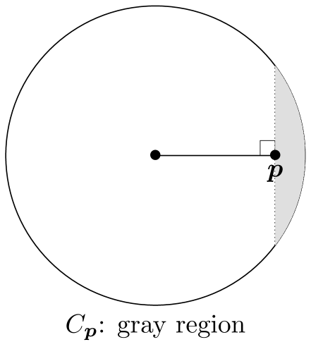
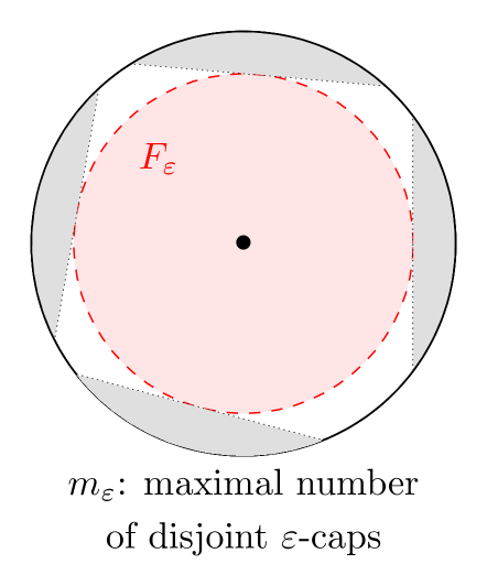
Figure 8: (Left) Cap induced by ${\boldsymbol{p}}\in\mathbb{B}^{2}$. (Middle) The $\varepsilon$-floating body is the complement of the union of $\varepsilon$-caps. (Right) The maximum number of independent $\varepsilon$-caps is denoted by $m_{\varepsilon}$.

Lemma 5.11.

Let $\mathsf{C}$ be an $\varepsilon$-cap. If $\varepsilon\to 0$, the radius $R_{\varepsilon}$ of $\mathsf{C}$ satisfies:

$$1-R_{\varepsilon}\sim c\,\varepsilon^{\frac{2}{d-1}}$$

Proof.

To ease the readability, we write $\mu(R)$ for $\mu(\mathsf{C})$ for any cap $\mathsf{C}$ of radius $R$ (due to rotational symmetry, $\mu(\mathsf{C})$ does only depend on the radius of $\mathsf{C}$, but not on $\mathsf{C}$ itself). We will compute $\mu(R)$, then inverse the formula to get an estimate for $R_{\varepsilon}$. With $C=C_{2,\frac{d}{2}-2}$, and letting $R\to 1$, we get:

$$\mu(R) =C\,\int_{x=R}^{1}\int_{y=-\sqrt{1-x^{2}}}^{+\sqrt{1-x^{2}}}\left(1-x^{2}-y^{2}\right)^{\beta}\,\mathrm{d}y\,\mathrm{d}x$$

$$=C\,\int_{R}^{1}\int_{\theta=-\arccos{r}}^{+\arccos{r}}(1-r^{2})^{\beta}\,r\mathrm{d}r\,\mathrm{d}\theta$$

$$=2\,C\,\int_{R}^{1}r\,(1-r^{2})^{\beta}\,\arccos{r}\,\mathrm{d}r$$

$$\sim 4\sqrt{2}\,C\,\int_{R}^{1}r\,(1-r^{2})^{\beta}\,\sqrt{1-r}\,\mathrm{d}r$$

$$\sim\frac{4\sqrt{2}\,C}{2\beta+3}\,(1-R)^{\frac{3}{2}}(1-R^{2})^{\beta}$$

$$\sim\frac{2^{\beta+\frac{5}{2}}\,C}{2\beta+3}\,(1-R)^{\beta+\frac{3}{2}}$$

We use: $\arccos{x}=\sqrt{2(1-x)}+o\left(1-x\right)$. The $5^{\text{th}}$ line is obtained with WolframAlpha and simplifications. If $R\to 1$, then $(1-R^{2})=(1+R)(1-R)\sim 2(1-R)$.

Finally, as $\varepsilon\to 0$ if and only if $R_{\varepsilon}\to 1$, it follows from $\mu(R_{\varepsilon})=\varepsilon$ that $1-R_{\varepsilon}=c\,\varepsilon^{\frac{1}{\beta+\frac{3}{2}}}$. Substituting $\beta=\frac{d}{2}-2$ finishes the proof. ∎

In the following, we will need to work with several independent $\varepsilon$-caps.

Definition 5.12.

Two caps $\mathsf{C},\mathsf{C}^{\prime}$ are said to be independent if they are disjoint, i.e., $\mathsf{C}\cap\mathsf{C}^{\prime}=\varnothing$. We denote by $m_{\varepsilon}$ the maximal number of pairwise independent $\varepsilon$-caps.

Proposition 5.13.

If $\varepsilon\to 0$, the maximal number $m_{\varepsilon}$ of independent $\varepsilon$-caps satisfies $m_{\varepsilon}\sim c\,\left(\frac{1}{\varepsilon}\right)^{\frac{1}{d-1}}$.

Proof.

Let $\alpha_{\varepsilon}$ be the half-angle spanned by an $\varepsilon$-cap, see picture below-right.

Then $m_{\varepsilon}\sim\frac{2\pi}{2\alpha_{\varepsilon}}$, and $\alpha_{\varepsilon}=\arccos{R_{\varepsilon}}$. Using Lemma˜5.11, and $\arccos{x}=\sqrt{2(1-x)}+o\left(1-x\right)$ if $x\to 1$, we get:

$$m_{\varepsilon}~\sim~\pi\,\left(\arccos{R_{\varepsilon}}\right)^{-1}~\sim~\frac{\pi}{\sqrt{2}}\,\left(\sqrt{1-R_{\varepsilon}}\right)^{-1}~\sim~\frac{\pi\,c}{\sqrt{2}}\,\left(\frac{1}{\varepsilon}\right)^{\frac{1}{d-1}}\qed$$

Inside an $\varepsilon$-cap

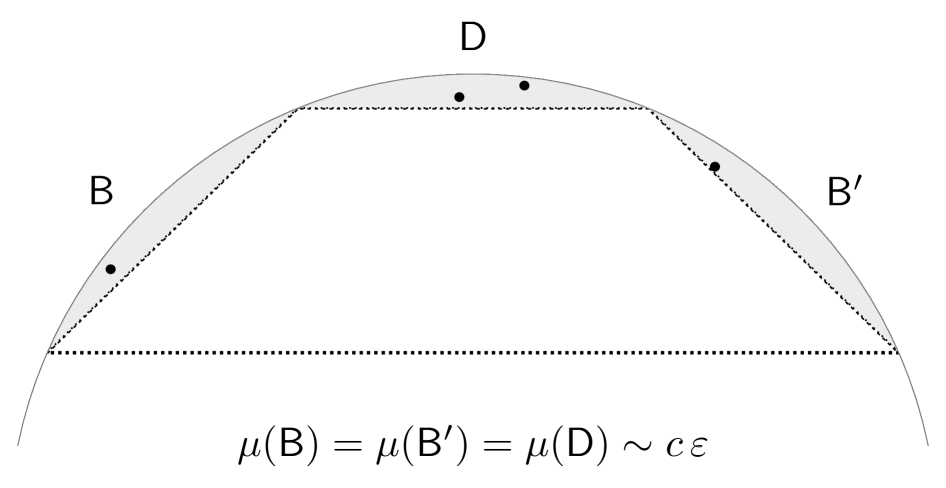
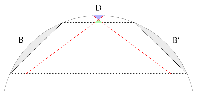
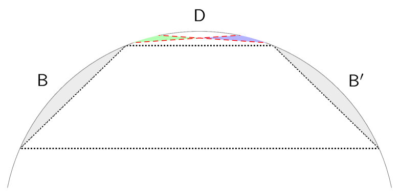
Figure 9: (Top) Definition of the subsets $\mathsf{B}$, $\mathsf{B}^{\prime}$ and $\mathsf{D}$, and event $A_{\mathsf{C}}$. (Bottom) Two sub-events with different $f_{0}(\mathsf{Q}_{n})$ that occur with strictly positive probability (see the proof of Proposition˜5.15).

To lower bound on the variance of $f_{0}(\mathsf{Q}_{n})$, we will consider certain local events (one for each $\varepsilon$-cap) that occur with strictly positive probability $p$, and are independent. We then show that, up to a constant, the variance is lower bounded by $p\cdot m_{\varepsilon}$. We now precise this strategy.

Definition 5.14.

For an $\varepsilon$-cap $\mathsf{C}$, let $\mathsf{B}$, $\mathsf{D}$ and $\mathsf{B}^{\prime}$ the three maximal sub-caps contained in $\mathsf{C}$, of the same measure, labeled from left to right, see Figure˜9 (Top). Remark that $\mathbb{B}^{2}\smallsetminus\mathsf{B}$ is convex, and so are $\mathbb{B}^{2}\smallsetminus\mathsf{B}^{\prime}$ and $\mathbb{B}^{2}\smallsetminus\mathsf{D}$. We will show that $\mu(\mathsf{B})=\mu(\mathsf{B}^{\prime})=\mu(\mathsf{D})\simeq c\,\varepsilon$ for some constant $c>0$ (even though this might feel surprising when looking at the picture, one needs to imagine that the cap $\mathsf{C}$ is very very slim, so the majority of the cap is indeed covered by the three sub-caps).

We let $A_{\mathsf{C}}$ be the event that, out of the random points $X_{1},\dots,X_{n}$, exactly one point belongs to $\mathsf{B}$ and $\mathsf{B}^{\prime}$ each, two points lie in $\mathsf{D}$, and all the other points lie outside the cap $\mathsf{C}$.

We compute $\mathbb{P}(A_{\mathsf{C}})$ and $\operatorname{Var}\bigl{(}f_{0}(\mathsf{Q}_{n})\,\big{|}\,A_{\mathsf{C}}\bigr{)}$. The latter is the variance of $f_{0}(\mathsf{Q}_{n})$, conditioned on the event $A_{\mathsf{C}}$, where all $X_{i}$ except the four ones achieving the event $A_{\mathsf{C}}$, are fixed.

Proposition 5.15.

Let $\varepsilon=c_{0}\frac{\log n}{n}$ with $c_{0}>0$. For an $\varepsilon$-cap $\mathsf{C}$, we have: $\mathbb{P}(A_{\mathsf{C}})\geq c\,(\log n)^{4}\,n^{-c_{0}}$.

Proof.

First, we compute $\mu(\mathsf{B})=\mu(\mathsf{B}^{\prime})=\mu(\mathsf{D})$. The half-angle $\theta_{\varepsilon}$ spanned by $\mathsf{B}$ is $\frac{1}{3}$ of the half-angle $\alpha_{\varepsilon}$ spanned by $\mathsf{C}$ (see the proof of Proposition˜5.13 for the definition of the half-angle). Thus $1-\cos\theta_{\varepsilon}\sim 1-\cos\frac{\alpha_{\varepsilon}}{3}\sim\frac{1}{3^{2}}\frac{\alpha_{\varepsilon}^{2}}{2}\sim\frac{1}{9}(1-\cos\alpha_{\varepsilon})$, where $\cos\alpha_{\varepsilon}$ is the radius of the cap $\mathsf{C}$ and $\cos\theta_{\varepsilon}$ the radius of the cap $\mathsf{B}$. By Lemma˜5.11, the measure of a cap of radius $R$ is $c\,(1-R^{\frac{2}{d-1}})$ for some $c>0$, so $\mu(\mathsf{B})\sim c\,9^{-\frac{2}{d-1}}(1-\cos\alpha_{\varepsilon})^{\frac{2}{d-1}}\sim 9^{-\frac{2}{d-1}}\mu(\mathsf{C})=9^{-\frac{2}{d-1}}\,\varepsilon$.

As all $X_{i}$ are independent, we have:

$$\mathbb{P}(A_{\mathsf{C}}) =\sum_{\{i,j,k,\ell\}\subseteq[n]}\mathbb{P}(X_{i}\in\mathsf{B})\mathbb{P}(X_{j}\in\mathsf{B}^{\prime})\mathbb{P}(X_{k}\in\mathsf{D})\mathbb{P}(X_{\ell}\in\mathsf{D})\prod_{g\notin\{i,j,k,\ell\}}\bigl{(}1-\mathbb{P}(X_{g}\in\mathsf{C})\bigr{)}$$

$$=\binom{n}{4}\bigl{(}\mu(\mathsf{B})\bigr{)}^{4}(1-\varepsilon)^{n-4}~~\sim\frac{c_{0}^{4}}{4!\cdot 9^{\frac{8}{d-1}}}\,(\log n)^{4}\,n^{-c_{0}}.$$

For the last estimate, we have used that $\varepsilon\to 0$ implies that $\log(1-\varepsilon)=-\varepsilon+o(\varepsilon)$, which yields $(1-\varepsilon)^{n}=\exp\left(n\cdot\left(-c_{0}\frac{\log n}{n}+o\left(\frac{\log n}{n}\right)\right)\right)\sim n^{-c_{0}}$. ∎

$\operatorname{Var}\bigl{(}f_{0}(\mathsf{Q}_{n})\,\big{|}\,A_{\mathsf{C}}\bigr{)}$ can be uniformly, i.e., independently of $\varepsilon$, bounded away from $0$ as follows:

Proposition 5.16.

There exists a constant $c>0$ such that for all $\varepsilon>0$ sufficiently small and any $\varepsilon$-cap $\mathsf{C}$, we have: $\operatorname{Var}\bigl{(}f_{0}(\mathsf{Q}_{n})\,\big{|}\,A_{\mathsf{C}}\bigr{)}\geq c$.

Proof.

Suppose $X_{1},\dots,X_{n}$ achieve the event $A_{\mathsf{C}}$. Let ${\boldsymbol{b}},{\boldsymbol{b}}^{\prime}$, and ${\boldsymbol{d}}_{1},{\boldsymbol{d}}_{2}$ the points among $X_{1},\dots,X_{n}$ which lie in $\mathsf{B}$, $\mathsf{B}^{\prime}$ and $\mathsf{D}$, respectively. As $\mathbb{B}^{2}\smallsetminus\mathsf{B}$ is convex, the point ${\boldsymbol{b}}$ is a vertex of$\mathsf{Q}_{n}=\operatorname{conv}(X_{i};i\in[n])$. Similarly, ${\boldsymbol{b}}^{\prime}$ and at least one of the points ${\boldsymbol{d}}_{1},{\boldsymbol{d}}_{2}$ are vertices of $\mathsf{Q}_{n}$.

Let $v$ be the number of vertices of $\mathsf{Q}_{n}$ that are different from ${\boldsymbol{b}},{\boldsymbol{b}}^{\prime},{\boldsymbol{d}}_{1}$ and ${\boldsymbol{d}}_{2}$. Then we have $f_{0}(\mathsf{Q}_{n})=v+3$ or $f_{0}(\mathsf{Q}_{n})=v+4$, depending on whether $\operatorname{conv}({\boldsymbol{b}},{\boldsymbol{b}}^{\prime},{\boldsymbol{d}}_{1},{\boldsymbol{d}}_{2})$ is a triangle or a quadrangle. The idea is to show, that both, $\mathbb{P}\bigl{(}\operatorname{conv}({\boldsymbol{b}},{\boldsymbol{b}}^{\prime},{\boldsymbol{d}}_{1},{\boldsymbol{d}}_{2})\text{ is a triangle}\bigr{)}$ and $\mathbb{P}\bigl{(}\operatorname{conv}({\boldsymbol{b}},{\boldsymbol{b}}^{\prime},{\boldsymbol{d}}_{1},{\boldsymbol{d}}_{2})\text{ is a quadrangle}\bigr{)}$ are strictly positive. It will follow that $f_{0}(\mathsf{Q}_{n})$ is not determined solely by $v$, implying that the variance of $f_{0}(\mathsf{Q}_{n})$ conditioned on $A_{\mathsf{C}}$ is strictly positive.

Consider two lines passing through the center of $\mathsf{D}$ and separating $\mathsf{B}$ from $\mathsf{B}^{\prime}$ (see red dashed lines in Figure˜9, bottom left): These lines divide $\mathsf{D}$ into four subsets, out of which two are separated from both $\mathsf{B}$ and $\mathsf{B}^{\prime}$ by these lines. We will call these subsets “top region” (blue) and “bottom region” (green). If ${\boldsymbol{d}}_{1}$ lies in the top region (blue), and ${\boldsymbol{d}}_{2}$ lies in the bottom region (green), then ${\boldsymbol{d}}_{2}\in\operatorname{conv}({\boldsymbol{b}},{\boldsymbol{b}}^{\prime},{\boldsymbol{d}}_{1})$ (for any ${\boldsymbol{b}}\in\mathsf{B}$, ${\boldsymbol{b}}^{\prime}\in\mathsf{B}^{\prime}$). This implies that $\operatorname{conv}({\boldsymbol{b}},{\boldsymbol{b}}^{\prime},{\boldsymbol{d}}_{1},{\boldsymbol{d}}_{2})$ is always a triangle in this case. Moreover, (conditioned on $A_{\mathsf{C}}$) the probability of this to happen is lower bounded by $\frac{\mu(\text{top region})\mu(\text{bottom region})}{\mu(\mathsf{D})^{2}}$. Since, restricted to $\mathsf{D}$, the $\beta$-distribution is close to the uniform distribution on $\mathsf{D}$ (for small $\varepsilon$), this quantity is strictly positive and can be bounded from below, independently of $\varepsilon$, by a strictly positive constant (roughly $\frac{1}{16}$ in the above figure).

Similarly, if ${\boldsymbol{d}}_{1}$ is in the right region (blue), and ${\boldsymbol{d}}_{2}$ in the left region (green) of Figure˜9 (bottom right), then $\operatorname{conv}({\boldsymbol{b}},{\boldsymbol{b}}^{\prime},{\boldsymbol{d}}_{1},{\boldsymbol{d}}_{2})$ is a quadrangle (for any ${\boldsymbol{b}}\in\mathsf{B}$, ${\boldsymbol{b}}^{\prime}\in\mathsf{B}^{\prime}$). By an analogous reasoning as above, this occurs with positive probability, that can be bounded away from $0$ (for any $\varepsilon$).

Consequently, $\operatorname{Var}\bigl{(}f_{0}(\mathsf{Q}_{n})\,\big{|}\,A_{\mathsf{C}}\bigr{)}$ is lower bounded by a positive constant. ∎

Lower bound on the variance

We can finally give a lower bound on the variance, combining Propositions˜5.13, 5.15 and 5.16.

Corollary 5.17.

For any $c_{0}>0$, there exists a constant $c>0$ such that:

$$\operatorname{Var}f_{0}(\mathsf{Q}_{n})\geq c\,n^{\frac{1}{d-1}-c_{0}}\quad\text{if }n\to+\infty.$$

Proof.

Let $\varepsilon=c_{0}\frac{\log(n)}{n}$ and let ${\mathcal{C}}=(\mathsf{C}_{1},\dots,\mathsf{C}_{m_{\varepsilon}})$ be a collection of $m_{\varepsilon}$ independent $\varepsilon$-caps.

For $\beta$-distributed points $X_{1},\dots,X_{n}$ , we let ${\boldsymbol{X}}\coloneqq\bigl{(}X_{i}~;~X_{i}\notin\mathsf{C}\text{ for all }\mathsf{C}\in{\mathcal{C}}~\text{with }{\boldsymbol{1}}(A_{\mathsf{C}})\bigr{)}$, where ${\boldsymbol{1}}(A)$ is the indicator function of the event $A$. Intuitively, ${\boldsymbol{X}}$ is the random variable consisting of those points of $(X_{1},\dots,X_{n})$ that are not involved in any of the events $A_{\mathsf{C}}$ that occur (for $\mathsf{C}\in{\mathcal{C}}$).

We will now use the law of total variance that we recall: if $Y$ and $Z$ are random variables (with $\operatorname{Var}Y<+\infty$), then $\operatorname{Var}Y=\mathbb{E}\bigl{(}\operatorname{Var}(Y~\big{|}~Z)\bigr{)}+\operatorname{Var}\bigl{(}\mathbb{E}(Y~\big{|}~Z)\bigr{)}$, where on the right-hand-side the expectancy and variance are conditioned on $Z$. In particular: $\operatorname{Var}Y\geq\mathbb{E}\bigl{(}\operatorname{Var}(Y~\big{|}~Z)\bigr{)}$. Applying this inequality to $Y=f_{0}(\mathsf{Q}_{n})$ and $Z={\boldsymbol{X}}$ yields: $\operatorname{Var}f_{0}(\mathsf{Q}_{n})\geq\mathbb{E}\bigl{(}\operatorname{Var}(f_{0}(\mathsf{Q}_{n})~\big{|}~{\boldsymbol{X}})\bigr{)}$.

To compute $\operatorname{Var}(f_{0}(\mathsf{Q}_{n})~\big{|}~{\boldsymbol{X}})$, first note that, for independent caps $\mathsf{C},\mathsf{C}^{\prime}\in{\mathcal{C}}$, the events $A_{\mathsf{C}}$ and $A_{\mathsf{C}^{\prime}}$ are independent. Moreover, if $A_{\mathsf{C}}$ and $A_{\mathsf{C}^{\prime}}$ are events with ${\boldsymbol{1}}(A_{\mathsf{C}})={\boldsymbol{1}}(A_{\mathsf{C}^{\prime}})=1$, then moving the points that are witnesses for $A_{\mathsf{C}}$, does not affect which of the points that witness $A_{\mathsf{C}^{\prime}}$ are vertices of $\mathsf{Q}_{n}$ and vice versa (as, for each cap $\mathsf{C}$, the sub-sets $\mathbb{B}^{2}\smallsetminus\mathsf{B}$, $\mathbb{B}^{2}\smallsetminus\mathsf{B}^{\prime}$ and $\mathbb{B}^{2}\smallsetminus\mathsf{D}$ are convex). Using this independence structure and Proposition˜5.16, we get that there is $c>0$ with:

$$\operatorname{Var}(f_{0}(\mathsf{Q}_{n})~\big{|}~{\boldsymbol{X}})~\geq~\sum_{\mathsf{C}\in{\mathcal{C}}}\operatorname{Var}(f_{0}(\mathsf{Q}_{n})~\big{|}~A_{\mathsf{C}})\,{\boldsymbol{1}}(A_{\mathsf{C}})~\geq~c\,\sum_{\mathsf{C}\in{\mathcal{C}}}{\boldsymbol{1}}(A_{\mathsf{C}})$$

Finally, by Propositions˜5.13 and 5.15, using $\varepsilon=c_{0}\frac{\log n}{n}$, we get that there exists $c^{\prime}>0$ with:

$$\begin{array}[]{rclcr}\operatorname{Var}f_{0}(\mathsf{Q}_{n})&\geq&\mathbb{E}\bigl{(}\operatorname{Var}(f_{0}(\mathsf{Q}_{n})~\big{|}~{\boldsymbol{X}})\bigr{)}&&\\ &\geq&c\,\sum_{\mathsf{C}\in{\mathcal{C}}}\mathbb{P}(A_{\mathsf{C}})~\geq~c\,m_{\varepsilon}\,\mathbb{P}(A_{\mathsf{C}_{1}})&&\\ &\geq&c^{\prime}\,\left(\frac{n}{\log n}\right)^{\frac{1}{d-1}}\,\,(\log n)^{4}\,n^{-c_{0}}&&\end{array}$$

As $(\log n)^{4-\frac{1}{d-1}}>1$ for large $n$, we can remove this term to get the claimed formula. ∎

$\varepsilon$-floating body and $\varepsilon$-visible region

In order to give an accurate upper bound for the variance of $f_{0}(\mathsf{Q}_{n})$, we will need to understand what happens when we “add a point” to $\mathsf{Q}_{n}$, and use the so-called Efron-Stein jackknife inequality (see next paragraph). Firstly, we want to measure how close the vertices of $\mathsf{Q}_{n}$ are to the boundary of the disk: To this end, we use the $\varepsilon$-floating body. Intellectually, the reader should think of it as a disk that is contained in $\mathsf{Q}_{n}$ with very high probability (for $n$ large enough): this help us rule out cases where $\mathsf{Q}_{n}$ is “far” from the circle $\mathbb{S}^{1}$. To be precise, suppose that $\mathsf{F}_{\varepsilon}\subseteq\mathsf{Q}_{n}$, then all the vertices of $\mathsf{Q}_{n}$ are in $\varepsilon$-caps. Reciprocally, fixing any $\varepsilon$-cap $\mathsf{C}$, the number of vertices of $\mathsf{Q}_{n}$ inside $\mathsf{C}$ is at least 1 (as $\mathsf{F}_{\varepsilon}$ is not contained in the interior of $\mathbb{B}^{2}\smallsetminus\mathsf{C}$), and roughly $\frac{\mu(\mathsf{C})}{\mu(\mathbb{B}^{2}\smallsetminus\mathsf{F}_{\varepsilon})}\,\mathbb{E}\bigl{(}f_{0}(\mathsf{P}_{n})\bigr{)}\sim c\,(\log n)^{\frac{1}{d-1}}$ (according to the next lemmas).

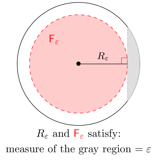
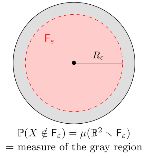
Figure 10: (Left) Cap induced by ${\boldsymbol{p}}\in\mathbb{B}^{2}$. (Middle) The $\varepsilon$-floating body is the complement of all $\varepsilon$-caps. (Right) With high probability, all the vertices and edges of $\mathsf{Q}_{n}$ are in the gray region.

Definition 5.18.

Let $\varepsilon>0$. The $\varepsilon$-floating body, see Figure˜10, is the complement of all $\varepsilon$-caps, i.e., $\mathsf{F}_{\varepsilon}$ $\coloneqq\mathbb{B}^{2}\smallsetminus\bigcup_{\mathsf{C}~\varepsilon\text{-cap}}\mathsf{C}=\{{\boldsymbol{p}}\in\mathbb{B}^{2}~;~\mu(\mathsf{C}_{{\boldsymbol{p}}})>\varepsilon\}$.

Remark 5.19.

The name floating body comes from the following idea: in the physical world, construct your favorite shape (here a disk) out of a material with a high buoyancy (e.g., foam), then immerse it in water and make it roll until every part that can be wet becomes wet. The part immersed at a given moment is the cap, and the part that remains forever dry is the floating body.

Lemma 5.20.

When $\varepsilon\to 0$, the $\varepsilon$-floating body is a disk of radius $R_{\varepsilon}$, satisfying $1-R_{\varepsilon}\sim c\,\varepsilon^{\frac{2}{d-1}}$.

Proof.

By rotational symmetry of the $\beta$-distribution, the floating body is a (possibly empty) disk (for all $\varepsilon$). If ${\boldsymbol{p}}$ is on the boundary of $\mathsf{F}_{\varepsilon}$, then $\mu(\mathsf{C}_{{\boldsymbol{p}}})=\varepsilon$, so Lemma˜5.11 implies the claim. ∎

Lemma 5.21.

The measure of the region outside the $\varepsilon$-floating body satisfies:

$$\mu(\mathbb{B}^{2}\smallsetminus\mathsf{F}_{\varepsilon})\sim c\,\varepsilon^{1-\frac{1}{d-1}}\quad\text{if }\varepsilon\to 0$$

Proof.

By Lemma˜5.11, the region $\mathbb{B}^{2}\smallsetminus\mathsf{F}_{\varepsilon}$ is an annulus of inner radius $R_{\varepsilon}$ and outer radius $1$. Hence, if $\varepsilon\to 0$, its measure according to the $\beta$-distribution is:

$$\mu(\mathbb{B}^{2}\smallsetminus\mathsf{F}_{\varepsilon})=C\,\int_{R_{\varepsilon}}^{1}2\pi\,(1-r^{2})^{\beta}\,r\mathrm{d}r~~=~\frac{\pi\,C}{\beta+1}\,(1-R_{\varepsilon}^{2})^{\beta+1}~~\sim~\frac{2^{\beta+1}\pi\,C}{\beta+1}\,(1-R_{\varepsilon})^{\beta+1}$$

Using $\beta=\frac{d}{2}-2$ and Lemma˜5.11, we get the claimed formula. ∎

Last but not least, we need to introduce the notion of visibility from a point.

Definition 5.22.

Let $\varepsilon>0$. For a point ${\boldsymbol{x}}\in\mathbb{B}^{2}$, the $\varepsilon$-visible region from ${\boldsymbol{x}}$ is the subset of the disk defined as: $\operatorname{vis_{\varepsilon}}{\boldsymbol{x}}$ $\coloneqq\{{\boldsymbol{y}}\in\mathbb{B}^{2}~;~[{\boldsymbol{x}},{\boldsymbol{y}}]\cap\mathsf{F}_{\varepsilon}=\varnothing\}$, see Figure˜11 (Left).

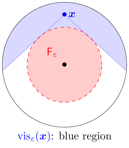
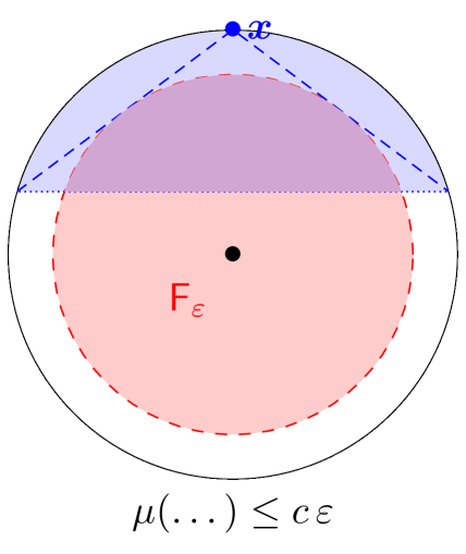
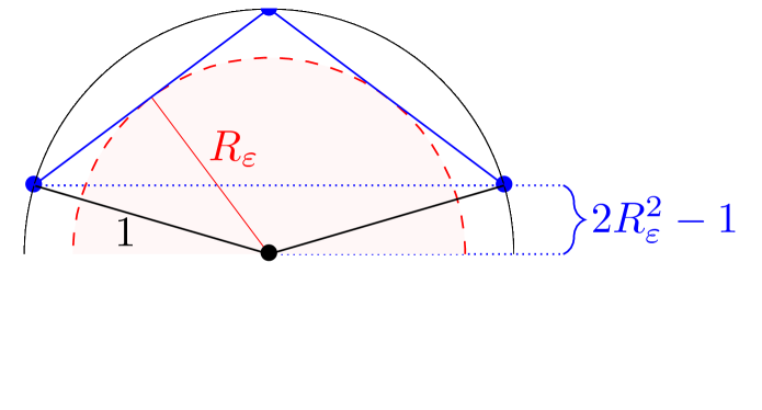
Figure 11: (Left) The $\varepsilon$-visible region from ${\boldsymbol{x}}$. (Middle) The biggest visibility region is achieved when ${\boldsymbol{x}}\in\mathbb{S}^{1}$. It is covered by the blue-shaded cap. (Right) The radius of this cap is $2R_{\varepsilon}^{2}-1$.

Lemma 5.23.

For ${\boldsymbol{x}}\in\mathbb{B}^{2}$, we have $\mu\bigl{(}\operatorname{vis_{\varepsilon}}{\boldsymbol{x}}\bigr{)}\sim c\,\varepsilon$, if $\varepsilon\to 0$.

Proof.

The measure of $\operatorname{vis_{\varepsilon}}{\boldsymbol{x}}$ is maximized when ${\boldsymbol{x}}\in\mathbb{S}^{1}$, see Figure˜11 (Middle). In this case, $\operatorname{vis_{\varepsilon}}{\boldsymbol{x}}$ is included in the cap $\mathsf{C}$ obtained by taking the two tangents to the disk $\mathsf{F}_{\varepsilon}$ passing through ${\boldsymbol{x}}$, and joining their points of intersection with $\mathbb{S}^{1}$. A quick scribble in the kite defined by these two points together with ${\boldsymbol{x}}$ and ${\boldsymbol{0}}$ gives that the radius defining this cap is $2R_{\varepsilon}^{2}-1$ if $\varepsilon$ is small enough, see Figure˜11 (Right). According to the proof of Lemma˜5.11, we get that $\mu(\mathsf{C})$ is of order $\bigl{(}1-(2R_{\varepsilon}^{2}-1)\bigr{)}^{\beta+\frac{3}{2}}$. As $R_{\varepsilon}\to 1$, we get $1-R_{\varepsilon}^{2}=(1+R_{\varepsilon})(1-R_{\varepsilon})\sim 2(1-R_{\varepsilon})$. Thus: $\mu(\mathsf{C})\sim c\,\bigl{(}2(1-R_{\varepsilon}^{2})\bigr{)}^{\beta+\frac{3}{2}}\sim 4^{\beta+\frac{3}{2}}\,c\,(1-R_{\varepsilon})^{\beta+\frac{3}{2}}\sim c^{\prime}\,\varepsilon$, where the last equivalence is Lemma˜5.11. ∎

We now show that, for large $n$, and $\varepsilon>0$ not too small, the $\varepsilon$-floating body is contained in $\mathsf{Q}_{n}$ with very high probability. To this end, we set $\varepsilon=c_{0}\,\frac{\log n}{n}$ for some $c_{0}>0$.

Proposition 5.24.

Let $c_{0}=\frac{1}{d-1}+s$, where $s>0$, and let $\varepsilon=c_{0}\frac{\log n}{n}$. We have

$$\mathbb{P}(\mathsf{F}_{\varepsilon}\not\subseteq\mathsf{Q}_{n})\leq c\,n^{-s}~~~~\text{ when }~~~~n\to+\infty$$

Proof.

Let $X_{1},\dots,X_{n}$ be i.i.d. according to the density $f_{2,\frac{d}{2}-2}$, and let $\mathsf{Q}_{n}=\operatorname{conv}(X_{1},\dots,X_{n})$.

If $\mathsf{F}_{\varepsilon}\not\subseteq\mathsf{Q}_{n}$, then there are two possibilities:

$(a)$ $\mathsf{Q}_{n}\subseteq\mathsf{F}_{\varepsilon}$;

$(b)$ there exists $X_{i}\notin\mathsf{F}_{\varepsilon}$ and an edge $\mathsf{e}$ incident to $X_{i}$ which intersects $\mathsf{F}_{\varepsilon}$.

Case $(a)$ amounts to $X_{j}\in\mathsf{F}_{\varepsilon}$ for all $j\in[n]$. For case $(b)$, let $\mathsf{C}_{i}$ be the $\varepsilon$-cap whose boundary line is parallel to $\mathsf{e}$ (see figure on the right). Since $\mathsf{e}$ is an edge, we have $X_{j}\notin\mathsf{C}_{i}$ for all $j\in[n]\setminus\{i\}$.

As $X_{1},\dots,X_{n}$ are independent, we get:

$$\begin{array}[]{rclcl}\mathbb{P}(\mathsf{F}_{\varepsilon}\not\subseteq\mathsf{Q}_{n})&=&\mathbb{P}(\mathsf{Q}_{n}\subseteq\mathsf{F}_{\varepsilon})&+&\mathbb{P}\bigl{(}\exists i\in[n],\,X_{i}\notin\mathsf{F}_{\varepsilon}~\text{ and }~\forall j\neq i,\,X_{j}\notin\mathsf{C}_{i}\bigr{)}\\ &\leq&\prod_{i=1}^{n}\mathbb{P}(X_{i}\in\mathsf{F}_{\varepsilon})&+&\sum_{i=1}^{n}\mathbb{P}(X_{i}\notin\mathsf{F}_{\varepsilon})\,\prod_{j\in[n]\setminus\{i\}}\mathbb{P}(X_{j}\notin\mathsf{C}_{i})\end{array}$$

For the asymptotics, when $n\to+\infty$, we use that by Lemma˜5.21 there exists a constant $c_{1}$ such that $\mathbb{P}(X_{i}\notin\mathsf{F}_{\varepsilon})\leq c_{1}\,\varepsilon^{1-\frac{1}{d-1}}$. Since $\mathbb{P}(X_{j}\notin\mathsf{C}_{i})=1-\mu(\mathsf{C}_{i})=1-\varepsilon$. We get:

$$\begin{array}[]{rclcl}\mathbb{P}(\mathsf{F}_{\varepsilon}\not\subseteq\mathsf{Q}_{n})&\leq&\left(1-c_{1}\,\varepsilon^{1-\frac{1}{d-1}}\right)^{n}&+&n\,\left(c_{1}\,\varepsilon^{1-\frac{1}{d-1}}\right)\,\left(1-\varepsilon\right)^{n-1}\\ \end{array}$$

Using that $\varepsilon=c_{0}\frac{\log n}{n}$ and $\log(1-x)\sim-x$ when $x\to 0$, for the first term on the right-hand side, we get: $\left(1-c_{1}\,\varepsilon^{1-\frac{1}{d-1}}\right)^{n}~\sim~\exp\left(-c_{1}c_{0}^{1-\frac{1}{d-1}}\,(\log n)^{1-\frac{1}{d-1}}\,n^{\frac{1}{d-1}}\right)$. And, for the second term on the right-hand side, we get: $n\,\left(c_{1}\,\varepsilon^{1-\frac{1}{d-1}}\right)\,\left(1-\varepsilon\right)^{n-1}~\sim~c_{1}\,(\log n)^{1-\frac{1}{d-1}}\,\exp\left(\left(\frac{1}{d-1}-c_{0}\right)\log n\right)$. The second term is easily seen to be asymptotically bigger than the first term when $n\to+\infty$. Hence, simplifying the last exponential, we get:

$$\mathbb{P}(\mathsf{F}_{\varepsilon}\not\subseteq\mathsf{Q}_{n})\leq c\,(\log n)^{1-\frac{1}{d-1}}\,n^{\frac{1}{d-1}-c_{0}}$$

By choosing $c_{0}=\frac{1}{d-1}+s$, we can ensure $\mathbb{P}(\mathsf{F}_{\varepsilon}\not\subseteq\mathsf{Q}_{n})\leq c\,n^{-s}$ for any fixed $s>0$. ∎

First order difference and Efron-Stein jackknife inequality

We now explain the main tools used to find an upper bound for the variance of $f_{0}(\mathsf{Q}_{n})$. The idea of the first order difference $Df_{0}(\mathsf{Q}_{n})$ is to measure the effect of the removal of a point from $n+1$ randomly chosen points on the number of vertices (or edges) of the convex hull of the random points: how many vertices have been lost or gained? (See Figure˜12 (Left): we count edges in figures, as it is easier to draw.)

Figure 12: (Left) Adding a new point $X_{1}$ to $\mathsf{Q}_{n}$ (green) creates 2 new edges (blue), and destroys 3 old edges (green dotted), so $D_{1}f_{1}(\mathsf{Q}_{n})=2-3=-1$ for this sample. (Right) The points in red are $\varepsilon$-visible from $X_{1}$ but not in the $\varepsilon$-floating body $\mathsf{F}_{\varepsilon}$.

To make things more precise, we first need to introduce some further notation. These notations will be re-employed when dealing with the central limit theorem in Section˜5.2.3. In order to make these notions reusable in other context, we chose to give a quite general presentation (though this might seem more complicated for readers non-versed in probability (e.g., us)).

Let $\mathbb{X}$ be a Polish space, for instance $\mathbb{X}$ can be a discrete space or an Euclidean space as $\mathbb{R}^{2}$. Let $f:\bigcup_{n=1}^{\infty}\mathbb{X}^{n}\to\mathbb{R}$ be a measurable function on the set of all (finite) ordered point configurations in $\mathbb{X}$. In our setting, $\mathbb{X}=\mathbb{B}^{2}$, and $f=f_{0}(\mathsf{Q}_{n})$.

The function $f$ is symmetric if for any permutation $\sigma\in{\mathcal{S}}_{n}$ and any $(x_{1},\ldots,x_{n})\in\mathbb{X}^{n}$, we get:

$$f(x_{1},\ldots,x_{n})=f(x_{\sigma(1)},\ldots,x_{\sigma(n)})$$

For $i\in[n]$ and ${\boldsymbol{x}}=(x_{1},\dots,x_{n})\in\mathbb{X}^{n}$, we let ${\boldsymbol{x}}^{i}$ $\coloneqq(x_{1},\dots,x_{i-1},x_{i+1},\dots,x_{n})$ the vector ${\boldsymbol{x}}$ with its $i^{\text{th}}$ coordinate removed.

Definition 5.25.

The first order difference operator of $f:\bigcup_{n=1}^{\infty}\mathbb{X}^{n}\to\mathbb{R}$ w.r.t. $i$ is defined as:

$$D_{i}f({\boldsymbol{x}})=f({\boldsymbol{x}})-f({\boldsymbol{x}}^{i})\quad\text{for }{\boldsymbol{x}}\in\mathbb{X}^{n}$$

If the choice of $i$ is irrelevant (e.g., if $f$ is symmetric), we write $Df({\boldsymbol{x}})$ instead of $D_{i}f({\boldsymbol{x}})$.

The Efron-Stein jackknife inequality provides an upper bound for the variance of certain random variables via the just introduced first order difference operators:

Theorem 5.26 ([20], [33, Sec. 3.2]).

Pick $X_{1},\dots,X_{n},X_{n+1}$ i.i.d. (according to a measure in a fixed convex body), and let $\mathsf{K}_{n}=\operatorname{conv}(X_{1},\dots,X_{n})$ and $\mathsf{K}_{n+1}=\operatorname{conv}(X_{1},\dots,X_{n},X_{n+1})$. Then for any real-valued symmetric function $f$, we have:

$$\operatorname{Var}f(\mathsf{K}_{n})\leq(n+1)\,\mathbb{E}\Bigl{(}\bigl{(}f(\mathsf{K}_{n+1})-f(\mathsf{K}_{n})\bigr{)}^{2}\Bigr{)}$$

Applying this inequality to our setting directly yields:

$$\operatorname{Var}f_{0}(\mathsf{Q}_{n})\leq(n+1)\,\mathbb{E}\Bigl{(}\bigl{(}Df_{0}(\mathsf{Q}_{n+1})\bigr{)}^{2}\Bigr{)}$$ (1)

Upper bound on the variance

Providing an upper bound for the variance (using Equation˜1), hence amounts to proving an upper bound for the second moment of $Df_{0}(\mathsf{Q}_{n})$. As the proof of the central limit theorem will also require upper bounds for the fourth moment, in the following, we will provide upper bounds for all moments of $Df_{0}(\mathsf{Q}_{n})$.

Theorem 5.27.

Let $p$ be a positive integer. There exists $c>0$ such that:

$$\mathbb{E}\bigl{(}|Df_{0}(\mathsf{Q}_{n})|^{p}\bigr{)}\leq c\,(\log n)^{p+1-\frac{1}{d-1}}\,\left(\frac{1}{n}\right)^{1-\frac{1}{d-1}}\quad\text{if }n\to+\infty$$

Proof.

Since either $\mathsf{F}_{\varepsilon}\subseteq\mathsf{Q}_{n}$ or $\mathsf{F}_{\varepsilon}\not\subseteq\mathsf{Q}_{n}$, we can split the expectancy as follows:

$$\mathbb{E}\bigl{(}|Df_{0}(\mathsf{Q}_{n})|^{p}\bigr{)}=\mathbb{E}\bigl{(}|Df_{0}(\mathsf{Q}_{n})|^{p}\,\big{|}\,\mathsf{F}_{\varepsilon}\not\subseteq\mathsf{Q}_{n}\bigr{)}\mathbb{P}(\mathsf{F}_{\varepsilon}\not\subseteq\mathsf{Q}_{n})~\,+\,~\mathbb{E}\bigl{(}|Df_{0}(\mathsf{Q}_{n})|^{p}\,\big{|}\,\mathsf{F}_{\varepsilon}\subseteq\mathsf{Q}_{n}\bigr{)}\mathbb{P}(\mathsf{F}_{\varepsilon}\subseteq\mathsf{Q}_{n})$$

By Proposition˜5.24, for $s>0$ and $c_{0}\geq\frac{1}{d-1}+s$, there exists a constant $c>0$ such that $\mathbb{P}(\mathsf{F}_{\varepsilon}\not\subseteq\mathsf{Q}_{n})\leq c\,n^{-s}$ for $\varepsilon=c_{0}\frac{\log n}{n}$. Besides, trivially: $|Df_{0}(\mathsf{Q}_{n})|\leq n$ (it is impossible to gain or lose more than $n$ vertices). Thus, the first term in the above equation is easily bounded as follows:

$$\mathbb{E}\bigl{(}|Df_{0}(\mathsf{Q}_{n})|^{p}\,\big{|}\,\mathsf{F}_{\varepsilon}\not\subset\mathsf{Q}_{n}\bigr{)}\mathbb{P}(\mathsf{F}_{\varepsilon}\not\subset\mathsf{Q}_{n})\leq c\,n^{p-s}$$

with $s>0$, $c_{0}$, $c$ and $\varepsilon$ as above.

Hence, using $\mathbb{P}(\mathsf{F}_{\varepsilon}\subseteq\mathsf{Q}_{n})\leq 1$, we are left to prove that $\mathbb{E}\bigl{(}|Df_{0}(\mathsf{Q}_{n})|^{p}\,\big{|}\,\mathsf{F}_{\varepsilon}\subseteq\mathsf{Q}_{n}\bigr{)}$ is upper bounded by the claimed formula.

Suppose that $\mathsf{F}_{\varepsilon}\subseteq\mathsf{Q}_{n}$. By symmetry, we only compute the first order difference operator with respect to $X_{1}$ to $\mathsf{Q}_{n}$, (see Figure˜12 Left). We distinguish two cases:

1. $X_{1}\in\operatorname{conv}(X_{2},\dots,X_{n})$: No vertices are removed or added, and hence $Df_{0}(\mathsf{Q}_{n})=0$.

2. $X_{1}\notin\operatorname{conv}(X_{2},\dots,X_{n})$: Two new edges appear, and $m$ edges are deleted. An upper bound for $m$ is given by the number of vertices of $\operatorname{conv}(X_{2},\dots,X_{n})$ in the $\varepsilon$-visible region of $X_{1}$, see Figure˜12 (Right). This yields $|Df_{0}(\mathsf{Q}_{n})|^{p}=|m-2|^{p}\leq\left(\sum_{i=2}^{n}{\boldsymbol{1}}(X_{i}\in\operatorname{vis_{\varepsilon}}X_{1})\right)^{p}$ $=\sum_{2\leq i_{1},\dots,i_{p}\leq n}\prod_{j}{\boldsymbol{1}}(X_{i_{j}}\in\operatorname{vis_{\varepsilon}}X_{1})$.

Note that, in the above product, certain variables $X_{i_{j}}$ can be repeated, but as all the variables $X_{i}$ are independent, we get $\mathbb{P}\left(\prod_{j}{\boldsymbol{1}}(X_{i_{j}}\in\operatorname{vis_{\varepsilon}}X_{1})=1\right)=\mu(\operatorname{vis_{\varepsilon}}X_{1})^{\#\{i_{1},\dots,i_{p}\}}$. Besides, if$X_{1}\notin\operatorname{conv}(X_{2},\dots,X_{n})$, then in particular $X_{1}\notin\mathsf{F}_{\varepsilon}$ (since we assumed $\mathsf{F}_{\varepsilon}\subseteq\mathsf{Q}_{n}$). Hence, $\mathbb{P}\bigl{(}X_{1}\notin\operatorname{conv}(X_{2},\dots,X_{n})\bigr{)}\leq\mathbb{P}(X_{1}\notin\mathsf{F}_{\varepsilon})$. Consequently, when $n\to+\infty$ (remember $p$ is fixed):

$$\mathbb{E}\bigl{(}|Df_{0}(\mathsf{Q}_{n})|^{p}\,\big{|}\,\mathsf{F}_{\varepsilon}\subseteq\mathsf{Q}_{n}\bigr{)} \leq 0~+~\mathbb{P}(X_{1}\notin\mathsf{F}_{\varepsilon})\,\sum_{2\leq i_{1},\dots,i_{p}\leq n}\mu(\operatorname{vis_{\varepsilon}}X_{1})^{\#\{i_{1},\dots,i_{p}\}}$$

$$\leq\mathbb{P}(X_{1}\notin\mathsf{F}_{\varepsilon})\,\sum_{q=1}^{p}\binom{n-1}{q}q^{p-q}\,\mu(\operatorname{vis_{\varepsilon}}X_{1})^{q}$$

$$\leq~c\,\mathbb{P}(X_{1}\notin\mathsf{F}_{\varepsilon})\,\sum_{q=1}^{p}n^{q}\,\mu(\operatorname{vis_{\varepsilon}}X_{1})^{q} \text{for some }c>0$$

Using Lemma˜5.21, we have $\mathbb{P}(X_{1}\notin\mathsf{F}_{\varepsilon})\leq c_{1}\,\varepsilon^{1-\frac{1}{d-1}}$ for some constant $c_{1}>0$. By Lemma˜5.23, we get $\mu(\operatorname{vis_{\varepsilon}}X_{1})\leq c_{2}\,\varepsilon$, for some constant $c_{2}>0$. So, taking $\varepsilon=c_{0}\frac{\log n}{n}$, the above sum is a polynomial in $(\log n)$ of degree $p$. Thus, as $p$ is fixed, when $n\to+\infty$, there exists $c>0$ with:

$$\mathbb{E}\bigl{(}|Df_{0}(\mathsf{Q}_{n})|^{p}\,\big{|}\,\mathsf{F}_{\varepsilon}\subseteq\mathsf{Q}_{n}\bigr{)}\leq c\,(\log n)^{p+1-\frac{1}{d-1}}\,\left(\frac{1}{n}\right)^{1-\frac{1}{d-1}}\qed$$

Combining Theorems˜5.26 and 5.27 with $p=2$ yields the desired upper bound for the variance.

Corollary 5.28.

When $n\to+\infty$, there exists a constant $c>0$ such that:

$$\operatorname{Var}f_{0}(\mathsf{Q}_{n})\leq c\,(\log n)^{3-\frac{1}{d-1}}\,n^{\frac{1}{d-1}}$$

5.2.3 Central limit theorem

Concentration

Knowledge about the variance and the expectancy of a sequence of positive random variables $(Z_{n})_{n\in\mathbb{N}}$ can be used to prove a concentration theorem (e.g., via Chebyshev’s inequality). In particular, if the variance is not of the same order of magnitude as the square of the expectancy, i.e., $\operatorname{Var}Z_{n}=o\bigl{(}(\mathbb{E}\,Z_{n})^{2}\bigr{)}$ if $n\to+\infty$, then $\operatorname{Var}\frac{Z_{n}}{\mathbb{E}\,Z_{n}}\to 0$, and the sequence $(Z_{n})_{n\in\mathbb{N}}$ is “highly concentrated around its expected sequence $(\mathbb{E}\,Z_{n})_{n\in\mathbb{N}}$”, meaning that with probability tending to $1$, the random variable $Z_{n}$ is very close to its expectancy when $n\to+\infty$.

Applying these ideas to $Z_{n}=f_{0}(\mathsf{Q}_{n})$ yields the following concentration inequality.

Corollary 5.29.

When $n\to+\infty$, $\operatorname{Var}f_{0}(\mathsf{Q}_{n})=o\Bigl{(}\bigl{(}\mathbb{E}f_{0}(\mathsf{Q}_{n})\bigr{)}^{2}\Bigr{)}$. Hence, for any fixed $a>0$:

$$\mathbb{P}\left(\left|\frac{f_{0}(\mathsf{Q}_{n})}{\mathbb{E}f_{0}(\mathsf{Q}_{n})}-1\right|~\geq~a\right)~\xrightarrow[n\to+\infty]{}~0$$

Proof.

Since $\mathbb{E}f_{0}(\mathsf{Q}_{n})\sim c\,n^{\frac{1}{d-1}}$, and $\operatorname{Var}f_{0}(\mathsf{Q}_{n})\leq c^{\prime}\,(\log n)^{3-\frac{1}{d-1}}\,n^{\frac{1}{d-1}}$, by Corollaries˜5.8 and 5.28, we have $\operatorname{Var}f_{0}(\mathsf{Q}_{n})=o\Bigl{(}\bigl{(}\mathbb{E}f_{0}(\mathsf{Q}_{n})\bigr{)}^{2}\Bigr{)}$. Applying Chebychev’s inequality for fixed $a>0$ yields:

$$\mathbb{P}\left(\left|\frac{f_{0}(\mathsf{Q}_{n})}{\mathbb{E}f_{0}(\mathsf{Q}_{n})}-1\right|\geq a\right)~=~\mathbb{P}\left(\bigl{|}f_{0}(\mathsf{Q}_{n})-\mathbb{E}f_{0}(\mathsf{Q}_{n})\bigr{|}\geq a\cdot\mathbb{E}f_{0}(\mathsf{Q}_{n})\right)~\leq~\frac{\operatorname{Var}f_{0}(\mathsf{Q}_{n})}{a^{2}\,\bigl{(}\mathbb{E}f_{0}(\mathsf{Q}_{n})\bigr{)}^{2}}\to 0$$

∎

A tool to control the distance to the Gaussian distribution

In order to prove a central limit theorem, we introduce a powerful tool from [35], which simplifies a previously known criterion from [27]. The main idea is to use certain quantities, similar to the ones defined to establish the variance in Section˜5.2.2, to control the Kolmogorov distance between the standard normal distribution and a certain statistic on random polytopes; in our case the number of vertices. Recall that the Kolmogorov distance between (real) random variables $X$ and $Y$ is the supremum of the difference of their cumulative distribution functions: $d_{\text{Kol}}(X,Y)$ $=\sup_{z\in\mathbb{R}}|\mathbb{P}(X\leq z)-\mathbb{P}(Y\leq z)|$.

We now describe the method explicitly. Although it seems notation heavy, the attentive reader will find strong similarity to Definition˜5.25 and consorts. As, once more, we want the readers to be able to re-use it at will, we introduce the tool from [35] in the general setting of a Polish space $\mathbb{X}$ (e.g., a discrete space or an Euclidean space), and a symmetric measurable function on the set of all point configuration on $\mathbb{X}$ that is $f:\bigcup_{n=1}^{\infty}\mathbb{X}^{n}\to\mathbb{R}$. For ${\boldsymbol{x}}=(x_{1},\dots,x_{n})$ and $i<j$, we let${\boldsymbol{x}}^{ij}$ $=(x_{1},\dots,x_{i-1},x_{i+1},\dots,x_{j-1},x_{j+1},\dots,x_{n})$ be the tuple ${\boldsymbol{x}}$ without its $i^{\text{th}}$ and $j^{\text{th}}$ coordinates.

Definition 5.30.

The second order difference operator of $f:\bigcup_{n=1}^{\infty}\mathbb{X}^{n}\to\mathbb{R}$ with respect to $i$ and $j$ is defined as:

$$D_{ij}f({\boldsymbol{x}})=f({\boldsymbol{x}})-f({\boldsymbol{x}}^{i})-f({\boldsymbol{x}}^{j})+f({\boldsymbol{x}}^{ij})\quad\text{for }{\boldsymbol{x}}\in\mathbb{X}^{n}$$

Recall that: $D_{i}f({\boldsymbol{x}})=f({\boldsymbol{x}})-f({\boldsymbol{x}}^{i})$ for $i\in[n]$. Intuitively, $D_{i}f({\boldsymbol{x}})$ measures the effect of the removal of the $i$^th component from ${\boldsymbol{x}}$ on $f$, whereas $D_{ij}f({\boldsymbol{x}})$ measures not only the effect of the removal of the $i$^th and $j$^th component from ${\boldsymbol{x}}$ but also their interaction.

Definition 5.31.

Let ${\boldsymbol{X}}=(X_{1},\dots,X_{n})$, ${\boldsymbol{X}}^{\prime}=(X^{\prime}_{1},\dots,X^{\prime}_{n})$ and $\widetilde{{\boldsymbol{X}}}=(\widetilde{X}_{1},\ldots,\widetilde{X}_{n})$ be vectors of i.i.d. random variables taking values on $\mathbb{X}^{n}$. A recombination of ${\boldsymbol{X}},{\boldsymbol{X}}^{\prime}$ and $\widetilde{{\boldsymbol{X}}}$ is a vector of random variables ${\boldsymbol{Z}}=(Z_{1},\dots,Z_{n})$, where $Z_{i}\in\{X_{i},X^{\prime}_{i},\widetilde{X}_{i}\}$ for $i\in[n]$.

For a symmetric measurable function $f:\bigcup_{n=1}^{\infty}\mathbb{X}^{n}\to\mathbb{R}$ and vectors of i.i.d. random variables ${\boldsymbol{X}},{\boldsymbol{X}}^{\prime}$ and $\widetilde{{\boldsymbol{X}}}$ taking values on $\mathbb{X}^{n}$, let $\gamma_{1}$, $\gamma_{2}$, $\gamma_{3}$ be defined as follows:

$$\gamma_{1}(f) \coloneqq\mathbb{E}\Bigl{(}|Df({\boldsymbol{X}})|^{4}\Bigr{)}$$

$$\gamma_{2}(f) \coloneqq\sup_{({\boldsymbol{Y}},{\boldsymbol{Z}})}\mathbb{E}\Bigl{(}{\boldsymbol{1}}\bigl{(}D_{12}f({\boldsymbol{Y}})\neq 0\bigr{)}\,D_{1}f({\boldsymbol{Z}})^{4}\Bigr{)}$$

$$\gamma_{3}(f) \coloneqq\sup_{({\boldsymbol{Y}},{\boldsymbol{Y}}^{\prime},{\boldsymbol{Z}})}\mathbb{E}\Bigl{(}{\boldsymbol{1}}\bigl{(}D_{12}f({\boldsymbol{Y}})\neq 0\bigr{)}\,{\boldsymbol{1}}\bigl{(}D_{13}f({\boldsymbol{Y}}^{\prime})\neq 0\bigr{)}\,D_{2}f({\boldsymbol{Z}})^{4}\Bigr{)}$$

where the suprema run over all $({\boldsymbol{Y}},{\boldsymbol{Z}})$ resp. $({\boldsymbol{Y}},{\boldsymbol{Y}}^{\prime},{\boldsymbol{Z}})$ that are recombinations of $\{{\boldsymbol{X}},{\boldsymbol{X}}^{\prime},\widetilde{{\boldsymbol{X}}}\}$.

With these definitions at hand, we can finally state the main tool explicitly.

Theorem 5.32 ([27], [35, Cor. 2.7]).

Let $X_{1},\ldots,X_{n}$ be independent random variables, identically distributed, taking values on a Polish space $\mathbb{X}$. For a symmetric measurable function $f:\bigcup_{n=1}^{\infty}\mathbb{X}^{n}\to\mathbb{R}$, let $W=f(X_{1},\ldots,X_{n})$ satisfying $\mathbb{E}(W)<\infty$ and $\mathbb{E}(W^{2})<\infty$.

Let $U\sim{\mathcal{N}}(0,1)$ be a standard Gaussian random variable. Then there exists $c>0$ such that:

$$d_{\mathrm{Kol}}\left(\frac{W-\mathbb{E}(W)}{\sqrt{\operatorname{Var}W}}\,,\,U\right)~\leq~c\,\,\frac{1}{\operatorname{Var}W}\left(\sqrt{n}\gamma_{1}(f)\,+\,n\sqrt{\gamma_{2}(f)}\,+\,n\sqrt{n}\sqrt{\gamma_{3}(f)}\right)$$ (2)

In the following, we will apply Theorem˜5.32 to $f=f_{0}(\operatorname{conv}(\cdot))$, and show that the right-hand side of (2) tends to $0$ when $n\to+\infty$.

Controlling $\operatorname{Var}$, $\gamma_{1}$, $\gamma_{2}$ and $\gamma_{3}$ for $f_{0}(\mathsf{Q}_{n})$

Firstly, $\operatorname{Var}f_{0}(\mathsf{Q}_{n})$ and $\gamma_{1}(f_{0}(\mathsf{Q}_{n}))$ have been tackled in Theorems˜5.27 and 5.17 (with $p=4$): for all $c_{0}>0$, there exists $c,c^{\prime}>0$ such that:

$$\operatorname{Var}\bigl{(}f_{0}(\mathsf{Q}_{n})\bigr{)}\geq c\,n^{\frac{1}{d-1}-c_{0}}~~\text{ and }~~\sqrt{n}\gamma_{1}\bigl{(}f_{0}(\mathsf{Q}_{n})\bigr{)}\leq c^{\prime}\,(\log n)^{5-\frac{1}{d-1}}\left(\frac{1}{n}\right)^{\frac{1}{2}-\frac{1}{d-1}}$$

To control $\gamma_{2}$ and $\gamma_{3}$, we need to understand the interaction of two points in our configuration.

Lemma 5.33.

For $\varepsilon>0$, and $X,Y\in\mathbb{B}^{2}$, there exists $c>0$ such that: $\mathbb{P}(\operatorname{vis_{\varepsilon}}X\cap\operatorname{vis_{\varepsilon}}Y\neq\varnothing)\leq c\,\varepsilon$.

Proof.

Let $P_{r}$ and $P_{\ell}$ be the right-most and left-most points of the arc $(\operatorname{vis_{\varepsilon}}X)\cap\mathbb{S}^{1}$. If we have $\operatorname{vis_{\varepsilon}}X\cap\operatorname{vis_{\varepsilon}}Y\neq\varnothing$, then in particular, $Y\in\bigl{(}\operatorname{vis_{\varepsilon}}X\cup\operatorname{vis_{\varepsilon}}P_{r}\cup\operatorname{vis_{\varepsilon}}P_{\ell}\bigr{)}$. With Lemma˜5.23 we conclude that there exists $c>0$ with $\mathbb{P}(\operatorname{vis_{\varepsilon}}X\cap\operatorname{vis_{\varepsilon}}Y\neq\varnothing)\leq 3\,c\,\varepsilon$. ∎

Remark 5.34.

Remark that we also have $\mathbb{P}(\operatorname{vis_{\varepsilon}}X\cap\operatorname{vis_{\varepsilon}}Y\neq\varnothing)\geq c^{\prime}\,\varepsilon$ for some $c^{\prime}>0$, since for any $Y\in\operatorname{vis_{\varepsilon}}X$, we get: $\operatorname{vis_{\varepsilon}}X\cap\operatorname{vis_{\varepsilon}}Y\neq\varnothing$, and Lemma˜5.23 ensures: $\mu(\operatorname{vis_{\varepsilon}}X)\geq c^{\prime}\,\varepsilon$.

Proposition 5.35.

There exists $c>0$ such that, when $n\to+\infty$, we have:

$$\gamma_{2}\bigl{(}f_{0}(\mathsf{Q}_{n})\bigr{)}\leq c\,(\log n)^{6-\frac{1}{d-1}}\,\left(\frac{1}{n}\right)^{2-\frac{1}{d-1}}$$

Proof.

Throughout this proof, let $\varepsilon=c_{0}\frac{\log n}{n}$ for some $c_{0}>0$ and let ${\boldsymbol{X}}=(X_{1},\dots,X_{n})$, ${\boldsymbol{X}}^{\prime}=(X^{\prime}_{1},\dots,X^{\prime}_{n})$ and $\widetilde{{\boldsymbol{X}}}=(\widetilde{X}_{1},\ldots,\widetilde{X}_{n})$ be random vectors as in Definition˜5.31, picked according to the $\beta$-distribution on $\mathbb{B}^{2}$. To simplify notation, we set $f({\boldsymbol{X}})\coloneqq f_{0}(\operatorname{conv}({\boldsymbol{X}}))$.

Let ${\boldsymbol{Y}}$ and ${\boldsymbol{Z}}$ be recombinations of ${\boldsymbol{X}},{\boldsymbol{X}}^{\prime}$ and $\widetilde{{\boldsymbol{X}}}$. In the following, we condition on the floating body being contained in the polygon at stake. More precisely, we let $A$ be the event that $\mathsf{F}_{\varepsilon}\subseteq\bigcap_{{\boldsymbol{W}}\in\{{\boldsymbol{Y}},{\boldsymbol{Z}}\}}\operatorname{conv}(W_{3},\dots,W_{n})$. Using Proposition˜5.24 and the union bound, we conclude that for any $s>0$, there exists $c^{\prime}>0$ such that $1-\mathbb{P}(A)\leq c^{\prime}\,(n-2)^{-s}\leq c^{\prime}n^{-s}$.

On the complement of the event $A$, we use the trivial bound $Df({\boldsymbol{Z}})^{4}\leq n^{4}$.

On the event $A$, we argue as follows: If $\operatorname{vis_{\varepsilon}}Y_{1}\cap\operatorname{vis_{\varepsilon}}Y_{2}=\varnothing$, then $\operatorname{conv}({\boldsymbol{Y}})\smallsetminus\operatorname{conv}({\boldsymbol{Y}}^{1})$ and $\operatorname{conv}({\boldsymbol{Y}})\smallsetminus\operatorname{conv}({\boldsymbol{Y}}^{2})$ do not intersect and hence, $D_{12}f({\boldsymbol{Y}})=0$. Lemma˜5.33 thus implies, that $\mathbb{P}(D_{12}f({\boldsymbol{Y}})\neq 0)\leq c\,\varepsilon$, for some $c>0$. Putting these arguments together, we obtain:

$$\begin{array}[]{rcll}\gamma_{2}(f)&\leq&\mathbb{P}(A)\,\mathbb{E}\Bigl{(}{\boldsymbol{1}}\bigl{(}D_{12}f({\boldsymbol{Y}})\neq 0\bigr{)}\,D_{2}f({\boldsymbol{Z}})^{4}\,\,\Big{|}\,\,A\Bigr{)}&+~\bigl{(}1-\mathbb{P}(A)\bigr{)}\,n^{4}\\ &\leq&1\cdot\mathbb{P}\bigl{(}\operatorname{vis_{\varepsilon}}Y_{1}\cap\operatorname{vis_{\varepsilon}}Y_{2}\neq\varnothing\bigr{)}\,\mathbb{E}\bigl{(}|Df({\boldsymbol{Z}})|^{4}\bigr{)}&+~c^{\prime}\,n^{4-s}\\ &\leq&c\,\varepsilon\,\mathbb{E}\bigl{(}|Df({\boldsymbol{Z}})|^{4}\bigr{)}&+~c^{\prime}\,n^{4-s}\end{array}$$

Finally, using Theorem˜5.27 (with $p=4$), and $\varepsilon=c_{0}\frac{\log n}{n}$, we get the claimed upper bound. ∎

Proposition 5.36.

There exists $c>0$ such that, when $n\to+\infty$, we have:

$$\gamma_{3}\bigl{(}f_{0}(\mathsf{Q}_{n})\bigr{)}\leq c\,(\log n)^{7-\frac{1}{d-1}}\,\left(\frac{1}{n}\right)^{3-\frac{1}{d-1}}$$

Proof.

The proof is very similar to the one of Proposition˜5.35 (up to multiplying once by $\varepsilon$), and we will use the same notation as therein. In particular, let ${\boldsymbol{Y}}$, ${\boldsymbol{Y}}^{\prime}$, ${\boldsymbol{Z}}$ be recombinations of ${\boldsymbol{X}},{\boldsymbol{X}}^{\prime}$ and $\widetilde{{\boldsymbol{X}}}$, and let $\varepsilon=c_{0}\frac{\log n}{n}$ for some $c_{0}>0$. Here, we consider the event $A$ of the floating body $\mathsf{F}_{\varepsilon}$ being contained in $\bigcap_{{\boldsymbol{W}}\in\{{\boldsymbol{Y}},{\boldsymbol{Y}}^{\prime},{\boldsymbol{Z}}\}}\operatorname{conv}(W_{4},\dots,W_{n})$. Again by Proposition˜5.24, for any $s>0$, there exists $c^{\prime}>0$ such that: $1-\mathbb{P}(A)\leq c^{\prime}\,n^{-s}$.

As before, if $\operatorname{vis_{\varepsilon}}Y_{1}\cap\operatorname{vis_{\varepsilon}}Y_{2}=\varnothing$, then $D_{12}f({\boldsymbol{Y}})=0$, and similarly for ${\boldsymbol{Y}}^{\prime}$. So, if $D_{12}f({\boldsymbol{Y}})\neq 0$ and $D_{12}f({\boldsymbol{Y}}^{\prime})\neq 0$, then both, $\operatorname{vis_{\varepsilon}}Y_{1}\cap\operatorname{vis_{\varepsilon}}Y_{2}\neq\varnothing$ and $\operatorname{vis_{\varepsilon}}Y^{\prime}_{1}\cap\operatorname{vis_{\varepsilon}}Y^{\prime}_{2}\neq\varnothing$. As these two events are independent, by Lemma˜5.33, they occur jointly with probability less than $c\,\varepsilon^{2}$ for $c>0$. Thus:

$$\begin{array}[]{rcll}\gamma_{3}(f)&\leq&\mathbb{P}(A)\,\mathbb{E}\Bigl{(}{\boldsymbol{1}}\bigl{(}D_{12}f({\boldsymbol{Y}})\neq 0\bigr{)}\,{\boldsymbol{1}}\bigl{(}D_{13}f({\boldsymbol{Y}}^{\prime})\neq 0\bigr{)}\,D_{2}f({\boldsymbol{Z}})^{4}\,\,\Big{|}\,\,A\Bigr{)}&+~\bigl{(}1-\mathbb{P}(A)\bigr{)}\,n^{4}\\ &\leq&1\cdot\mathbb{P}\bigl{(}\operatorname{vis_{\varepsilon}}Y_{1}\cap\operatorname{vis_{\varepsilon}}Y_{2}\neq\varnothing\bigr{)}\,\mathbb{P}\bigl{(}\operatorname{vis_{\varepsilon}}Y^{\prime}_{1}\cap\operatorname{vis_{\varepsilon}}Y^{\prime}_{2}\neq\varnothing\bigr{)}\,\mathbb{E}\bigl{(}|Df({\boldsymbol{Z}})|^{4}\bigr{)}&+~c^{\prime}\,n^{4-s}\\ &\leq&c\,\varepsilon^{2}\,\mathbb{E}\bigl{(}|Df({\boldsymbol{Z}})|^{4}\bigr{)}&+~c^{\prime}\,n^{4-s}\end{array}$$

Finally, using Theorem˜5.27 (with $p=4$), and $\varepsilon=c_{0}\frac{\log n}{n}$, we get the claimed upper bound. ∎

Corollary 5.37.

Let $X_{1},\dots,X_{n}$ be $\beta$-distributed points in the disk $\mathbb{B}^{2}$ with $\beta=\frac{d}{2}-2$, and let $\mathsf{Q}_{n}=\operatorname{conv}(X_{1},\dots,X_{n})$. Let $U\sim{\mathcal{N}}(0,1)$ be a standard Gaussian random variable. Then:

$$d_{\mathrm{Kol}}\left(\frac{f_{0}(\mathsf{Q}_{n})-\mathbb{E}f_{0}(\mathsf{Q}_{n})}{\sqrt{\operatorname{Var}f_{0}(\mathsf{Q}_{n})}}\,,\,U\right)\xrightarrow[n\to+\infty]{}0$$

Proof.

By Theorems˜5.27, 5.17, 5.35 and 5.36, we have that for $f_{0}(\mathsf{Q}_{n})$, the quantities $\frac{1}{\operatorname{Var}}$, $\sqrt{n}\gamma_{1}$, $n\gamma_{2}$ and $n\sqrt{n}\gamma_{3}$ can all be upper bounded by terms of the form $(\log n)^{a}\left(\frac{1}{n}\right)^{b}$ with $b$ as follows (recall that, in Corollary˜5.17, there is no restriction on $c_{0}>0$):

quantity	$\frac{1}{\operatorname{Var}(\cdot)}$	$\sqrt{n}\gamma_{1}$	$n\sqrt{\gamma_{2}}$	$n\sqrt{n}\sqrt{\gamma_{3}}$
$b$	$\frac{1}{d-1}-c_{0}$ for any $c_{0}>0$	$\frac{1}{2}-\frac{1}{d-1}$	$\frac{-1}{2(d-1)}$	$\frac{-1}{2(d-1)}$

Hence the sum $\frac{1}{\operatorname{Var}}\left(\sqrt{n}\gamma_{1}\,+\,n\sqrt{\gamma_{2}}\,+\,n\sqrt{n}\sqrt{\gamma_{3}}\right)$ is upper bounded by $c\,(\log n)^{a}\,\left(\frac{1}{n}\right)^{\frac{1}{2(d-1)}-c_{0}}$ for some $c>0$, any $c_{0}>0$, and $a=\frac{7}{2}-\frac{1}{2(d-1)}$. By Theorem˜5.32, choosing $c_{0}$ sufficiently small guarantees that the Kolmogorov distance at stake tends to $0$. ∎

Remark 5.38.

This corollary holds for any $\beta$-distribution in the plane, with $\beta>0$.

We end this section by providing the proof of Theorem˜5.1

Proof of Theorem˜5.1

Proof of Theorem˜5.1.

By Corollary˜5.5, the random variables $L(\omega,\mathsf{P}_{n})$, $f_{0}^{\text{up}}(\mathsf{Q}_{n})$ and $f_{0}^{\text{low}}(\mathsf{Q}_{n})$ have the same distribution. Since $f_{0}(\mathsf{Q}_{n})=f_{0}^{\text{up}}(\mathsf{Q}_{n})+f_{0}^{\text{low}}(\mathsf{Q}_{n})$, we get: $\mathbb{E}L(\omega,\mathsf{P}_{n})=\frac{1}{2}\mathbb{E}f_{0}(\mathsf{Q}_{n})$. We need to control the variance of $L(\omega,\mathsf{P}_{n})$. We are going to prove that $\operatorname{Var}L(\omega,\mathsf{P}_{n})\sim\frac{1}{2}\operatorname{Var}f_{0}(\mathsf{Q}_{n})$ by showing that $f_{0}^{\text{up}}(\mathsf{Q}_{n})$ and $f_{0}^{\text{low}}(\mathsf{Q}_{n})$ are “almost independent”. Firstly:

$$\operatorname{Var}f_{0}(\mathsf{Q}_{n})=\operatorname{Var}f_{0}^{\text{up}}(\mathsf{Q}_{n})\,+\,\operatorname{Var}f_{0}^{\text{low}}(\mathsf{Q}_{n})\,+\,\mathrm{Cov}\Bigl{(}f_{0}^{\text{up}}(\mathsf{Q}_{n}),\,f_{0}^{\text{low}}(\mathsf{Q}_{n})\Bigr{)}$$

For $1\leq k\leq n$, let $V_{j}^{\text{up}}$ (resp. $V_{j}^{\text{low}}$) be the event that the point $X_{j}$ is an upper (resp. lower) vertex (i.e., it has an outer normal vector with positive, resp. negative, second coordinate). Then:

$$\mathrm{Cov}\Bigl{(}f_{0}^{\text{up}}(\mathsf{Q}_{n}),\,f_{0}^{\text{low}}(\mathsf{Q}_{n})\Bigr{)}=\sum_{j,k=1}^{n}\mathrm{Cov}\Bigl{(}{\boldsymbol{1}}(V_{j}^{\text{up}}),\,{\boldsymbol{1}}(V_{k}^{\text{low}})\Bigr{)}$$

As per usual, we control the vertices using the floating body.

Suppose $\mathsf{F}_{\varepsilon}\subseteq\mathsf{Q}_{n}$. If $X_{j}$ and $X_{k}$ (for $k\neq j$) are not contained in a common $\varepsilon$-cap, then the events “$X_{j}$ is a vertex of $\mathsf{Q}_{n}$” and “$X_{k}$ is a vertex of $\mathsf{Q}_{n}$” are independent (because$X_{k}\in\operatorname{conv}(X_{i}~;~i\neq k)$ is equivalent to $X_{k}\in\operatorname{conv}(X_{i}~;~i\neq k\text{ and }i\neq j)$). Thus, if both events $V^{\text{up}}_{j}$ and $V^{\text{low}}_{k}$ occur, then both $X_{j}$ and $X_{k}$ lie in an $\varepsilon$-cap which contains upper and lower vertices, in particular, this $\varepsilon$-cap is contained in the visibility region of $(-1,0)$ or of $(1,0)$.

Finally, we use that the covariance of $\bigl{(}f_{0}^{\text{up}}(\mathsf{Q}_{n}),\,f_{0}^{\text{low}}(\mathsf{Q}_{n})\bigr{)}$, conditioned on $\mathsf{F}_{\varepsilon}\not\subseteq\mathsf{Q}_{n}$, is smaller than $\binom{n}{2}$. Using $\varepsilon=c_{0}\frac{\log n}{n}$, Lemmas˜5.23 and 5.24, there exists $c>0$ satisfying:

$$\left|\mathrm{Cov}\Bigl{(}f_{0}^{\text{up}}(\mathsf{Q}_{n}),\,f_{0}^{\text{low}}(\mathsf{Q}_{n})\Bigr{)}\right|\,\leq\,\binom{n}{2}\mathbb{P}(\mathsf{F}_{\varepsilon}\not\subseteq\mathsf{Q}_{n})\,+\,\binom{n}{2}\Bigl{(}2\mu\bigl{(}\operatorname{vis_{\varepsilon}}(-1,0)\bigr{)}\Bigr{)}^{2}\mathbb{P}(\mathsf{F}_{\varepsilon}\subseteq\mathsf{Q}_{n})\,\leq\,c\,(\log n)^{2}$$

As $(\log n)^{2}=o\bigl{(}\operatorname{Var}f_{0}(\mathsf{Q}_{n})\bigr{)}$, and $\operatorname{Var}f_{0}^{\text{up}}(\mathsf{Q}_{n})=\operatorname{Var}f_{0}^{\text{low}}(\mathsf{Q}_{n})$, due to their distribution being identical, we get that $\operatorname{Var}L({\boldsymbol{\omega}},\mathsf{P}_{n})=\operatorname{Var}f_{0}^{\text{up}}(\mathsf{Q}_{n})\sim\frac{1}{2}\operatorname{Var}f_{0}(\mathsf{Q}_{n})$.

It remains to show that $f_{0}^{\text{up}}(\mathsf{Q}_{n})$ admits a central limit theorem. Sadly, this cannot be deduced directly from the central limit theorem for $f_{0}^{\text{up}}(\mathsf{Q}_{n})$. However, the attentive reader will easily notice that replacing $f_{0}$ by $f_{0}^{\text{up}}$ in Section˜5.2.3 (and Theorem˜5.27) only changes the constants, not the dependencies in $n$. Consequently, one can control the Kolmogorov distance between (the normalization of) $f_{0}^{\text{up}}(\mathsf{Q}_{n})$ and a standard normal distributed variable, finally proving Theorem˜5.1.

∎

Some open problems

We finish by proposing open problems which naturally extend what we discussed in this section.

Problem 5.39.

Compute the higher moments of $L_{n}$, the length of the coherent path (for fixed ${\boldsymbol{c}}$ and ${\boldsymbol{\omega}}$) on random polytopes. Equivalently, compute the higher moments of the number of vertices of $\beta$-distributed polygons. Moreover, prove a stronger convergence of $\frac{L_{n}-\mathbb{E}\,L_{n}}{\sqrt{\operatorname{Var}L_{n}}}$ towards the standard normal distribution, e.g., a convergence in moments.

Problem 5.40.

Sample points $X_{1},\dots,X_{n}$ at random, uniformly on the $(d-1)$-sphere, and construct $\mathsf{P}_{n}=\operatorname{conv}(X_{1},\dots,X_{n})$. For ${\boldsymbol{c}}={\boldsymbol{e}}_{1}$, let $N^{\text{coh}}_{\ell}$ be the number of coherent paths of length $\ell$ on $\mathsf{P}_{n}$. Study the probability for $(N^{\text{coh}}_{\ell})_{\ell}$ to be unimodal (conjecturally, it tends to $1$ when $n\to+\infty$).

Problem 5.41.

Sample points $X_{1},\dots,X_{n}$ at random, uniformly on the $(d-1)$-sphere, and construct $\mathsf{P}_{n}=\operatorname{conv}(X_{1},\dots,X_{n})$. Study the number of coherent paths on $\mathsf{P}_{n}$ (distribution, expectancy, variance, central limit theorem).

Problem 5.42.

Sample points $X_{1},\dots,X_{n}$ at random, uniformly on the $(d-1)$-sphere, and construct $\mathsf{P}_{n}=\operatorname{conv}(X_{1},\dots,X_{n})$. Study the number and the length of ${\boldsymbol{e}}_{1}$-monotone paths on $\mathsf{P}_{n}$.

Problem 5.43.

Extend the results of this paper to similar probability distributions, and especially to the polar case: random polytopes defined by $\mathsf{P}^{\circ}_{n}=\{{\boldsymbol{x}}\in\mathbb{R}^{d}~;~\left<{\boldsymbol{x}},{\boldsymbol{a}}_{i}\right>\leq 1\text{ for all }i\in[m]\}$ where the facet normals ${\boldsymbol{a}}_{1},\dots,{\boldsymbol{a}}_{m}$ are chosen uniformly at random on the sphere $\mathbb{S}^{d-1}$.

5.3 Cheat sheet of formulas

Here is a quick overview of the main formulas and notations which appeared throughout Section˜5. The proofs and formal definitions are not given in this sub-section, please see the referred locations. All “$c$” denote positive constants (independent of $\beta$, $d$, $n$, $\varepsilon$, etc) which are not equal from one line to the other.

Probabilistic model

Section˜5.1

$X_{1},\dots,X_{n}$, random points in $\mathbb{B}^{2}$, i.i.d., $\beta$-distributed

$f_{2,\beta_{d}}({\boldsymbol{x}})=C_{2,\beta_{d}}\Bigl{(}1-\|{\boldsymbol{x}}\|\Bigr{)}^{\beta_{d}}$ for $\ x\in\mathbb{B}^{2}$

$\mu(A)$: measure of $A\subseteq\mathbb{B}^{2}$ according to the density function $f_{2,\beta_{d}}$

$\beta_{d}=\frac{1}{2}d-2$

$\mathsf{Q}_{n}=\operatorname{conv}(X_{1},\dots,X_{n})$: random $\beta$-polygon

$f_{0}(\mathsf{Q}_{n})$: number of vertices of $\mathsf{Q}_{n}$

Expectancy

Section˜5.2.1

$\mathbb{E}\bigl{(}f_{0}(\mathsf{Q}_{n})\bigr{)}\sim c\,n^{\frac{1}{d-1}}$

Variance

Section˜5.2.2

$\varepsilon=c_{0}\frac{\log n}{n}$: it is a definition

$1-R_{\varepsilon}\sim c\,\varepsilon^{\frac{2}{d-1}}$: radius of $\varepsilon$-cap and floating body

$m_{\varepsilon}\sim c\,\left(\frac{1}{\varepsilon}\right)^{\frac{1}{d-1}}$: maximal number of independent (i.e., disjoint) $\varepsilon$-caps

$\mathbb{P}(A_{\mathsf{C}})\geq c\,(\log n)^{4}\,n^{-c_{0}}$: probability of having 4 points “correctly placed” in an $\varepsilon$-cap

$\mathbb{P}(X\notin\mathsf{F}_{\varepsilon})=\mu(\mathbb{B}^{2}\smallsetminus\mathsf{F}_{\varepsilon})\sim c\,\varepsilon^{1-\frac{1}{d-1}}$: measure of the of the part outside the floating body

$\mu\bigl{(}\operatorname{vis_{\varepsilon}}{\boldsymbol{x}}\bigr{)}\sim c\,\varepsilon$: measure of the visibility region

$\mathbb{P}(\mathsf{F}_{\varepsilon}\not\subseteq\mathsf{Q}_{n})\leq c\,n^{-s}$, for any $s>0$ (requires $c_{0}=\frac{1}{d-1}+s$)

$\mathbb{E}\bigl{(}|Df_{0}(\mathsf{Q}_{n})|^{p}\bigr{)}\leq c\,(\log n)^{p+1-\frac{1}{d-1}}\,\left(\frac{1}{n}\right)^{1-\frac{1}{d-1}}$ where $D$ is (any) first order difference operator

$c\,n^{\frac{1}{d-1}-c_{0}}~\leq~\operatorname{Var}f_{0}(\mathsf{Q}_{n})~\leq~c^{\prime}\,(\log n)^{3-\frac{1}{d-1}}\,n^{\frac{1}{d-1}}$: for any $c_{0}>0$

(the lower bound does not require that $\mathsf{F}_{\varepsilon}\subseteq\mathsf{Q}_{n}$, i.e., $c_{0}>0$ can be arbitrarily small)

Central limit theorem

Section˜5.2.3

With $f({\boldsymbol{X}})=f_{0}(\operatorname{conv}({\boldsymbol{X}}))$

$\gamma_{1}(f)=\mathbb{E}\Bigl{(}|Df({\boldsymbol{X}})|^{4}\Bigr{)}~\leq~c^{\prime}\,(\log n)^{5-\frac{1}{d-1}}\left(\frac{1}{n}\right)^{1-\frac{1}{d-1}}$

$\gamma_{2}(f)=\sup_{({\boldsymbol{Y}},{\boldsymbol{Z}})}\mathbb{E}\Bigl{(}{\boldsymbol{1}}\bigl{(}D_{12}f({\boldsymbol{Y}})\neq 0\bigr{)}\,D_{1}f({\boldsymbol{Z}})^{4}\Bigr{)}~\leq~c\,(\log n)^{6-\frac{1}{d-1}}\,\left(\frac{1}{n}\right)^{2-\frac{1}{d-1}}$

$\gamma_{3}(f)=\sup_{({\boldsymbol{Y}},{\boldsymbol{Y}}^{\prime},{\boldsymbol{Z}})}\mathbb{E}\Bigl{(}{\boldsymbol{1}}\bigl{(}D_{12}f({\boldsymbol{Y}})\neq 0\bigr{)}\,{\boldsymbol{1}}\bigl{(}D_{13}f({\boldsymbol{Y}}^{\prime})\neq 0\bigr{)}\,D_{2}f({\boldsymbol{Z}})^{4}\Bigr{)}~\leq~c\,(\log n)^{7-\frac{1}{d-1}}\,\left(\frac{1}{n}\right)^{3-\frac{1}{d-1}}$

$d_{\text{Kol}}\left(\frac{f_{0}(\mathsf{Q}_{n})-\mathbb{E}f_{0}(\mathsf{Q}_{n})}{\sqrt{\operatorname{Var}f_{0}(\mathsf{Q}_{n})}}\,,\,U\right)~\leq~c\,(\log n)^{\frac{7}{2}-\frac{1}{2(d-1)}}\,\left(\frac{1}{n}\right)^{\frac{1}{2(d-1)}}~\xrightarrow[n\to+\infty]{}0$, where $U\sim{\mathcal{N}}(0,1)$

6 Algorithms for monotone paths and coherent paths

Monotone paths

The naive idea for counting ${\boldsymbol{c}}$-monotone paths on a polytope $\mathsf{P}$ according to their lengths is to enumerate (asking your favorite library of your favorite programming language) all monotone paths of the graph $G_{\mathsf{P},{\boldsymbol{c}}}$, and to record their lengths. Actually, the usual algorithm to enumerate monotone paths in a graph can directly be adapted to sort them by length. The time complexity is $O(f_{1})$, where $f_{1}$ is the number of edges of $\mathsf{P}$.

The algorithm works as follows: First, find a topological order on $G_{\mathsf{P},{\boldsymbol{c}}}$, i.e., label the vertices of $G_{\mathsf{P},{\boldsymbol{c}}}$ with ${\boldsymbol{v}}_{1},\dots,{\boldsymbol{v}}_{n}$ such that $i<j$ if ${\boldsymbol{v}}_{i}\to{\boldsymbol{v}}_{j}$. Given this order, for any $1\leq i\leq n$ and for any outgoing arc ${\boldsymbol{v}}_{i}\to{\boldsymbol{v}}_{j}$, the number of monotone paths of length $\ell$ using the edge ${\boldsymbol{v}}_{i}\to{\boldsymbol{v}}_{j}$ equals the number of paths of length $\ell-1$ from ${\boldsymbol{v}}_{1}$ to ${\boldsymbol{v}}_{i}$. This algorithm can be formalized as follows:

Data: Polytope $\mathsf{P}\subset\mathbb{R}^{d}$ with $n$ vertices, direction ${\boldsymbol{c}}\in\mathbb{R}^{d}$

Result: List $L$ such that $L(\ell)$ is the number of ${\boldsymbol{c}}$-monotone paths of length $\ell$ on $\mathsf{P}$

$G_{\mathsf{P},{\boldsymbol{c}}}\leftarrow\bigl{(}$directed graph of $\mathsf{P}$ where ${\boldsymbol{u}}\to{\boldsymbol{v}}$ iff $\left<{\boldsymbol{u}},{\boldsymbol{c}}\right><\left<{\boldsymbol{v}},{\boldsymbol{c}}\right>\bigr{)}$;

Relabel the nodes of $G_{\mathsf{P},{\boldsymbol{c}}}$ according to a topological order from ${\boldsymbol{v}}_{1}$ to ${\boldsymbol{v}}_{n}$;

for $i$ from $1$ to $n$ do

    $L_{i}\leftarrow[0,\dots,0]$ ;

     /* the list $L_{i}$ is indexed from $0$ to $n$ */

   

end for

$L_{1}(0)\leftarrow 1$;

for $i$ from $1$ to $n-1$ do

    for $j$ such that there is an out-going edge ${\boldsymbol{v}}_{i}\to{\boldsymbol{v}}_{j}\in G_{\mathsf{P},{\boldsymbol{c}}}$ do

       $L_{j}(\ell)\leftarrow L_{j}(\ell)+L_{i}(\ell-1)$     for $\ell\in[1,n]$

    end for

   

end for

Output: $L_{n}$

Algorithm 1 Counting ${\boldsymbol{c}}$-monotone paths on $\mathsf{P}$ according to length

Coherent paths

There are two usual ways to check if a monotone path is coherent. Recall that a ${\boldsymbol{c}}$-monotone path on $\mathsf{P}$ is coherent if and only if there is ${\boldsymbol{\omega}}$ to capture it, i.e., if the upper faces of the projection of $\mathsf{P}$ onto the plane spanned by ${\boldsymbol{c}}$ and ${\boldsymbol{\omega}}$ is (the projection of) the monotone path.

First method: Let $({\boldsymbol{u}}_{1},\dots,{\boldsymbol{u}}_{r})$ be the vertices of the monotone path to be tested for coherence. Being the upper faces of a2-dimensional polytope $\mathsf{P}_{{\boldsymbol{c}},{\boldsymbol{\omega}}}$ is easy to check inductively: suppose we know that ${\boldsymbol{u}}_{1},\dots,{\boldsymbol{u}}_{i}$ are upper vertices of $\mathsf{P}_{{\boldsymbol{c}},{\boldsymbol{\omega}}}$ for some given $i<r$, then the next upper vertex is the neighbor ${\boldsymbol{v}}$ of ${\boldsymbol{u}}_{i}$ which maximizes the slope in the plane ${\boldsymbol{c}}$ and ${\boldsymbol{\omega}}$, i.e., we need to find ${\boldsymbol{u}}_{i+1}$ that maximizes $\frac{\left<{\boldsymbol{\omega}},{\boldsymbol{v}}-{\boldsymbol{u}}_{i}\right>}{\left<{\boldsymbol{c}},{\boldsymbol{v}}-{\boldsymbol{u}}_{i}\right>}$ under the conditions that ${\boldsymbol{u}}_{i}{\boldsymbol{v}}$ is an edge of $\mathsf{P}$ and $\left<{\boldsymbol{u}}_{i},{\boldsymbol{c}}\right><\left<{\boldsymbol{v}},{\boldsymbol{c}}\right>$. This yields several inequalities (maximizing the slope amounts to be greater than all other slopes) which are linear in ${\boldsymbol{\omega}}$. We can hence gather all these linear inequalities to make a cone and the path is coherent if and only if this cone is full-dimensional.

Figure 13:  Projection of $\mathsf{P}$ onto a plane (not all edges are drawn). If ${\boldsymbol{u}}_{1},{\boldsymbol{u}}_{2},{\boldsymbol{u}}_{3}$ are upper vertices, then to compute the next vertex, one lists the right-neighbors of ${\boldsymbol{u}}_{3}$ (not in gray: ${\boldsymbol{u}}_{4},{\boldsymbol{u}}_{5},{\boldsymbol{u}}_{8},{\boldsymbol{u}}_{9}$), and finds the slope-maximizer from ${\boldsymbol{u}}_{3}$: here ${\boldsymbol{u}}_{4}$.

The algorithm is easy to write. It creates a cone in dimension $d$ with $O(f_{1})$ inequalities, where $f_{1}$ is the number of edges of $\mathsf{P}$. As far as we know, even if improvements exist, the time complexity remains bound to finding a vector in the interior of such a cone, hence it is $O(d^{2}\,f_{1})$.

Second method: Let $\mathsf{M}_{\mathsf{P},{\boldsymbol{c}}}$ be the monotone path polytope of polytope $\mathsf{P}$ and direction ${\boldsymbol{c}}$, see [15, 5, 9] for definitions, or [31, Section 2.1] for constructions of monotone path polytopes. The idea is that for ${\boldsymbol{\omega}},{\boldsymbol{\omega}}^{\prime}\in\mathbb{R}^{d}$, the vertices $\mathsf{M}_{\mathsf{P},{\boldsymbol{c}}}^{{\boldsymbol{\omega}}}$ and $\mathsf{M}_{\mathsf{P},{\boldsymbol{c}}}^{{\boldsymbol{\omega}}^{\prime}}$ are the same if and only if the coherent paths captured by ${\boldsymbol{\omega}}$ and ${\boldsymbol{\omega}}^{\prime}$ are the same. The next algorithm uses this key concept.

The time complexity is driven by the computation of the monotone path polytope. One method is to compute $n-2$ Minkowski sums in dimension $d$ (for $d$-dimensional polytope with $n$ vertices). Even though very costly, most libraries dealing with polytopes carry already-implemented efficient algorithms for doing so: this is enough for our use-case.

Data: Polytope $\mathsf{P}\subset\mathbb{R}^{d}$, direction ${\boldsymbol{c}}\in\mathbb{R}^{d}$, and ${\boldsymbol{c}}$-monotone path $({\boldsymbol{u}}_{1},\dots,{\boldsymbol{u}}_{r})$ on $\mathsf{P}$

Result: Boolean answer to “$({\boldsymbol{u}}_{1},\dots,{\boldsymbol{u}}_{r})$ is coherent?”, and certificate ${\boldsymbol{\omega}}$ if true

$\mathsf{C}\leftarrow\operatorname{cone}\Bigl{\{}{\boldsymbol{\omega}}\in\mathbb{R}^{d}~;~\forall i\in[r-1],~\forall{\boldsymbol{v}}\text{ improving neighbor of }{\boldsymbol{u}}_{i},~\frac{\left<{\boldsymbol{\omega}},{\boldsymbol{u}}_{i+1}-{\boldsymbol{u}}_{i}\right>}{\left<{\boldsymbol{c}},{\boldsymbol{u}}_{i+1}-{\boldsymbol{u}}_{i}\right>}\geq\frac{\left<{\boldsymbol{\omega}},{\boldsymbol{v}}-{\boldsymbol{u}}_{i}\right>}{\left<{\boldsymbol{c}},{\boldsymbol{v}}-{\boldsymbol{u}}_{i}\right>}\Bigr{\}}$

Output: Boolean: $\dim\mathsf{C}=d$; certificate: ${\boldsymbol{\omega}}\in\text{interior}(\mathsf{C})$

Algorithm 2 Checking if a monotone path is coherent

Data: Polytope $\mathsf{P}\subset\mathbb{R}^{d}$, direction ${\boldsymbol{c}}\in\mathbb{R}^{d}$

Result: List of all ${\boldsymbol{c}}$-coherent paths on $\mathsf{P}$ (with certificates)

$\mathsf{M}_{\mathsf{P},{\boldsymbol{c}}}$, Paths, Certificates $\leftarrow$ monotone path polytope of $\mathsf{P}$ for the direction ${\boldsymbol{c}}$, $[\,]$, $[\,]$

for ${\boldsymbol{v}}$ a vertex of $\mathsf{M}_{\mathsf{P},{\boldsymbol{c}}}$ do

    ${\boldsymbol{\omega}}\leftarrow$ a vector in the interior of the normal cone of ${\boldsymbol{v}}$

   Paths is appended the list of upper vertices of the projection of $\mathsf{P}$ in the plane $({\boldsymbol{c}},{\boldsymbol{\omega}})$

   Certificates is appended ${\boldsymbol{\omega}}$

end for

Output: Paths, Certificates

Algorithm 3 Finding all the coherent paths via the monotone path polytope

Universität Osnabrück, Germany

E-mail, M. Juhnke: martina.juhnke@uni-osnabrueck.de  ;    G. Poullot: germain.poullot@uni-osnabrueck.de

References

- ABB+ [23] Igor Araujo, Alexander E. Black, Amanda Burcroff, Yibo Gao, Robert A. Krueger, and Alex McDonough. Realizable standard young tableaux, 2023.
- ADLZ [22] Christos A. Athanasiadis, Jesús A. De Loera, and Zhenyang Zhang. Enumerative problems for arborescences and monotone paths on polytope graphs. J. Graph Theory, 99(1):58–81, 2022.
- AER [00] Christos A. Athanasiadis, Paul H. Edelman, and Victor Reiner. Monotone paths on polytopes. Math. Z., 235(2):315–334, 2000.
- AHRV [07] Omer Angel, Alexander E. Holroyd, Dan Romik, and Bálint Virág. Random sorting networks. Adv. Math., 215(2):839–868, 2007.
- ALRS [00] Christos A. Athanasiadis, Jesús A. De Loera, Victor Reiner, and Francisco Santos. Fiber polytopes for the projections between cyclic polytopes. European Journal of Combinatorics, 21(1):19–47, jan 2000.
- AS [01] Christos A. Athanasiadis and Francisco Santos. Monotone paths on zonotopes and oriented matroids. Canad. J. Math., 53(6):1121–1140, 2001.
- BDLL [21] Moïse Blanchard, Jesús A. De Loera, and Quentin Louveaux. On the length of monotone paths in polyhedra. SIAM J. Discrete Math., 35(3):1746–1768, 2021.
- BFRV [09] K.J. Böröczky, Ferenc Fodor, Matthias Reitzner, and Viktor Vígh. Mean width of random polytopes in a reasonably smooth convex body. Journal of Multivariate Analysis, 100:2287–2295, 11 2009.
- BL [23] Alexander Black and Jesús De Loera. Monotone paths on cross-polytopes. Discrete & Computational Geometry, 70:1245 – 1265, 2023.
- Bla [24] Alexander Black. Monotone paths on polytopes: Combinatorics and optimization. PhD thesis, 2024.
- BLKS [21] Alexander Black, Jesús A. De Loera, Sean Kafer, and Laura Sanità. On the simplex method for 0/1-polytopes. Mathematics of Operations Research, 2021.
- Bor [87] Karl-Heinz Borgwardt. The simplex method: A probabilistic analysis, volume 1 of Algorithms and Combinatorics: Study & Research Texts. Springer-Verlag, Berlin, 1987.
- Brä [15] Petter Bränden. Unimodality, log-concavity, real-rootedness and beyond. Handbook of Combinatorics, pages 437–483, 2015.
- BRT [21] Florian Besau, Daniel Rosen, and Christoph Thäle. Random inscribed polytopes in projective geometries. Math. Ann., 381(3-4):1345–1372, 2021.
- BS [92] Louis J. Billera and Bernd Sturmfels. Fiber polytopes. Anals of Mathematics, (135):527–549, 1992.
- BS [24] Alexander E. Black and Raman Sanyal. Underlying flag polymatroids. Adv. Math., 453:Paper No. 109835, 42, 2024.
- Dan [63] George B. Dantzig. Linear programming and extensions. Princeton University Press, Princeton, NJ, 1963.
- Dau [22] Duncan Dauvergne. The Archimedean limit of random sorting networks. J. Amer. Math. Soc., 35(4):1215–1267, 2022.
- DF [24] Samantha Dahlberg and Susanna Fishel. Maximal chains in lattices from graph associahedra: Tamari to the weak order, 2024.
- ES [81] B. Efron and C. Stein. The Jackknife Estimate of Variance. The Annals of Statistics, 9(3):586 – 596, 1981.
- KK [17] S. I. Kalmykov and D. B. Karp. Log-concavity and Turán-type inequalities for the generalized hypergeometric function. Anal. Math., 43(4):567–580, 2017.
- KM [72] Victor Klee and George J. Minty. How good is the simplex algorithm? In Inequalities, III (O. Shisha, editor), pages 159–175. Academic Press, New York-London, 1972.
- KS [10] D. Karp and S. M. Sitnik. Log-convexity and log-concavity of hypergeometric-like functions. J. Math. Anal. Appl., 364(2):384–394, 2010.
- KT [81] D. G. Kelly and J. W. Tolle. Expected number of vertices of a random convex polyhedron. SIAM J. Algebraic Discrete Methods, 2(4):441–451, 1981.
- KTZ [20] Zakhar Kabluchko, Christoph Thäle, and Dmitry Zaporozhets. Beta polytopes and poisson polyhedra: f-vectors and angles. Advances in Mathematics, 374:107333, 2020.
- Lod [04] Jean-Louis Loday. Realization of the Stasheff polytope. Archiv der Mathematik, 83(3):267–278, 2004.
- LRP [17] Raphaël Lachièze-Rey and Giovanni Peccati. New Berry–Esseen bounds for functionals of binomial point processes. The Annals of Applied Probability, 27(4):1992 – 2031, 2017.
- MSS [20] Sebastian Manecke, Raman Sanyal, and Jeonghoon So. S-hypersimplices, pulling triangulations, and monotone paths, 2020.
- MV [15] Colin Mallows and Robert J. Vanderbei. Which Young tableaux can represent an outer sum? J. Integer Seq., 18(9):Article 15.9.1, 8, 2015.
- Nel [17] Luke Nelson. A recursion on maximal chains in the tamari lattices. Discrete Mathematics, 340(4):661–677, 2017.
- Pou [24] Germain Poullot. Vertices of the monotone path polytopes of hypersimplicies, 2024.
- PSZ [23] Vincent Pilaud, Francisco Santos, and Günter M. Ziegler. Celebrating Loday’s associahedron. Archiv der Mathematik, 121(5):559–601, 2023.
- Rei [03] Matthias Reitzner. Random polytopes and the Efron–Stein jackknife inequality. The Annals of Probability, 31(4):2136 – 2166, 2003.
- Rei [05] Matthias Reitzner. Central limit theorems for random polytopes. Probability Theory and Related Fields, 133:483–507, 2005.
- SZ [25] Qi-Man Shao and Zhuo-Song Zhang. Berry-esseen bounds for functionals of independent random variables. Stochastic Processes and their Applications, 183:104574, 2025.
- Thä [18] Christoph Thäle. Central limit theorem for the volume of random polytopes with vertices on the boundary. Discrete Comput. Geom., 59(4):990–1000, 2018.
- TTW [18] Christoph Thäle, Nicola Turchi, and Florian Wespi. Random polytopes: central limit theorems for intrinsic volumes. Proc. Amer. Math. Soc., 146(7):3063–3071, 2018.