Quasinormal Modes and Shadows of Black Holes in Infinite Derivative Theory of Gravity

Abstract

In this work, we study the quasinormal modes (QNMs) and shadow of a Schwarzschild black hole (BH) with higher-order metric corrections, in the framework of the Infinite Derivative theory of Gravity (IDG). We study the effects of corrections to the BH’s metric, which arises from the IDG’s corrections, on the QNMs and shadow of the BH. We used the 6th-order Padé averaged WKB approximation method to study the QNMs of the BH perturbed by a scalar field. The dependence of the amplitude and damping of QNMs with respect to the free parameters has been analysed. It is found that the BH system becomes unstable for some values of the free parameters. We also studied the time evolution of a scalar field around the BH spacetime. The QNMs have also been calculated from the time profile of the evolution, which show good agreement with the values obtained from the WKB method. The variation of the shadow radius of the BH due to the inclusion of higher-order corrections has been studied. Finally, we constrain the free parameters associated with the correction terms using the data from the Keck and VLTI observation, and we obtain some bounds on the parameters.

I Introduction

General Relativity (GR) has been the most successful theory of gravity from its beginning. It has been extensively tested through various experiments and astronomical observations, which confirmed its predictions with high precision. The recent detection of gravitational waves (GWs) by the LIGO collaboration [1, 2, 3, 4, 5] and the groundbreaking images of black holes (BHs) captured lately by the Event Horizon Telescope (EHT) group [6, 7, 8, 9, 10, 11] stand as two remarkable milestones in this direction. However, despite its successes GR has been facing several fundamental challenges. As an example, we can say that GR struggles to explain why the Universe is expanding at an accelerated rate and why a significant portion of its mass seems to be missing [12, 13, 14, 15]. Similarly, when gravity is viewed as a fundamental interaction, at a very high energy scale where the quantum effects of gravity become dominant, GR fails to incorporate the Quantum Gravity (QG) effects into its solutions. The Standard Model (SM) of particle physics successfully describes the three fundamental interactions: strong, electromagnetic and weak interactions, in the framework of Quantum Field Theory (QFT), but it is unable to incorporate the gravitational interaction within it because GR is not a renormalizable theory. The quest to merge GR with SM continues to be an area of active research, and new theoretical constructs show increasing promise. Thus, QG theories [16, 17, 18, 19, 20, 21] are being formulated to bridge the gap between GR and QFT. Loop Quantum Gravity (LQG) [22, 23, 24, 25] and String Theory [26, 27, 28, 29, 30] are two widely studied theories in this direction. String Theory tries to unify the four fundamental interactions of nature in a single framework. String theory predicts the existence of a particle called graviton, which is the mediator of gravitational interaction. On the other hand, LQG only deals with quantizing gravity. In LQG, spacetime is quantized into discrete loops or quanta.

Although LQG and String Theory have been widely studied to investigate the QG approaches, their predictions have not been tested yet. The fact is that to test the predictions of String Theory and LQG, an enormous amount of energy, far beyond current experimental facilities is needed, which limits the experimental verification of these theories to an unachievable task. Because of this difficult challenge, alternative approaches have been looked into to study QG effects. One such approach is the framework of the Effective Field Theory (EFT). The EFT provides a way to explore QG effects within the energy scale accessible to current experiments without requiring extremely high energies. By treating GR as an effective theory of gravity valid up to a certain cut-off, this approach allows us to incorporate quantum corrections while maintaining consistency with GR at low energy. Several studies have been performed by considering GR as an EFT [31, 32, 33, 34, 35, 36]. It is to be noted that although EFT can predict only the low energy quantum corrections to a system and these low energy effects are very small, these effects become significant in extreme gravity regions such as near the event horizon of a BH or in the early Universe. The most promising testing ground for these theories with our current understanding lies in the extreme environments surrounding BHs. Accordingly, a number of studies have been done on the BHs in the framework of EFT [37, 38, 39, 40, 41, 42, 43, 44, 45].

Considering GR as an EFT, we can incorporate the low energy QG effects into the solutions of Einstein field equations, and hence we can test our calculations using the observational data obtained from BHs and Cosmic Microwave Background (CMB) [46, 47]. Since traditional approaches of EFT ignore the contributions from the high energy scale, we require some modifications to traditional EFTs to cover the UV incompleteness. Recently, the Infinite Derivative theory of Gravity (IDG) [48, 49] has gained significant attention due to its remarkable properties. This framework offers an asymptotically free and ghost-free extension of GR, ensuring that the only propagating degree of freedom in spacetime is the massless graviton. Moreover, IDG is considered as a promising candidate for UV complete modifications of GR, as its nonlocal structure helps to suppress divergences at high energy scales, potentially resolving singularities within the theory. The theory incorporates all possible higher derivative terms that are quadratic in curvature into the Einstein-Hilbert action, leading to modifications of Einstein’s gravity at short distances. Furthermore, such a higher derivative formulation naturally arises in String Field Theory (SFT), where it emerges as a consequence of higher-order $\alpha^{\prime}$ corrections [50], refining the gravitational dynamics at small scales.

Studying BH’s observables in such a theory can give us valuable information about how gravity behaves at the quantum scale. By analyzing these observables, one can test whether our current theories hold or not. BH thermodynamics provides a key framework where gravity, quantum physics and thermodynamics intersect, which is significant in unveiling the quantum aspect of gravity. Observation of BH phase shifts and changes in entropy can provide additional information on QG. These measurable quantities not only help to test the validity of existing theories but also guide the development of new models that aim to unify GR with quantum physics. BH thermodynamics have been extensively studied in Refs. [51, 52, 53, 54, 55, 56, 57, 58, 59] from the perspectives of different theories of gravity.

The quasinormal modes (QNMs) of BHs allow the direct extraction of the frequency associated with the characteristic oscillation of the BHs. These oscillation frequencies are dependent on the mass, spin, and charge of the BHs and can be altered due to the impact of the QG effects acting on the BH spacetime. In many approaches to QG, such as LQG and String Theory, modifications to the classical BH metric lead to shifts in QNM frequencies. Additionally, the AdS/CFT correspondence suggests a deep connection between QNMs and the relaxation timescales of strongly coupled QFTs [60, 61]. This duality implies that understanding the QNMs in asymptotically AdS spacetime can provide insights into the quantum properties of gravity. Because of these reasons, the study of QNMs of BHs can provide QG signatures around the BH spacetime. The QNMs of BHs have been studied extensively in different theories of gravity in recent times [62, 63, 64, 65, 66, 67, 68, 69, 70, 71].

Similarly, the study of the BH shadow offers valuable information on the quantum nature of gravity. The nature of BH shadows is based on the spacetime geometry, which is affected by quantum corrections. In various QG models, modifications to the BH metric lead to deviations in the shadow’s size and shape from GR predictions. In LQG, corrections to the Schwarzschild or Kerr metric can result in a slightly altered photon sphere, leading to measurable changes in the shadow’s angular diameter [72, 73, 74]. The study of BH shadow is also linked to the holographic principle, which suggests that gravity in higher-dimensional spacetime can be described by a lower-dimensional QFT [75, 76]. The EHT provides us the opportunity to observe the BH shadows and analyze the differences between predictions made with classical GR and the inclusion of possible effects of QG. The various studies on shadows of BH based on different forms of theories of gravity are currently available in the literature [77, 78, 79, 80, 81, 82, 83].

Inspired by the above mentioned factors, our work aims to study the QNMs and shadows of BHs in the framework of IDG. Specifically, a recent development in relation to BH solutions within this theoretical framework [84] has inspired us to investigate the QNMs and shadows of the BHs in this gravity framework. To calculate the QNMs we implement the Padé averaged 6th-order WKB approximation method and for the study of shadows, we adopt the techniques used in Refs. [52, 85, 86].

Our work is organized as follows: In Section II, we briefly discuss IDG and the solution of Schwarzschild BHs in this framework of gravity. In Section III, we compute the QNMs of the BHs. In Section IV, we study the evolution of a scalar field perturbation around our considered BHs spacetime and calculate the QNMs of the BHs using time domain analysis of the evolution. In Section V, we study the shadows of the BHs. In Section VI, we summarize and conclude our work.

II Infinite derivative Gravity and Schwarzschild Black Holes

IDG is a modification of GR that incorporates an infinite number of curvature derivatives into the Einstein-Hilbert action, distinguishing it from conventional higher-derivative gravity theories [87, 88]. As mentioned earlier the motivation behind the development of IDG was to construct a theory free from ghosts and singularities. Moreover, IDG exhibits better UV behavior than other higher-derivative gravity theories because its specific nonlocal modifications lead to an exponential suppression of high-energy modes while avoiding ghosts. The details of the derivations of the field equations and BH solutions in IDG are available in the literature [84, 49]. In this section, we highlight some important steps of those derivations.

The most general form of the action with second order in curvature is given by [84, 48, 49]

$$S=\int{d^{4}x}\sqrt{-g}\left[\frac{R}{16\pi}+RF_{1}(\Box)R+R_{\mu\nu}F_{2}(\Box)R^{\mu\nu}+C_{\mu\nu\sigma\rho}F_{3}(\Box)C^{\mu\nu\sigma\rho}\right],$$ (1)

where $g_{\mu\nu}$ is the spacetime metric, $\Box$ is the d’Alemberian operator, $R$ is the Ricci scalar, $R_{\mu\nu}$ is the Ricci tensor and $C_{\mu\nu\sigma\rho}$ is the Weyl tensor. $F_{1}$, $F_{2}$ and $F_{3}$ are analytic functions and are given by

$$F_{i}(\Box)=\sum_{n\,=\,0}^{\infty}f_{i,n}{\Box}^{n}.$$ (2)

Here, $f_{i,n}$ are Taylor series coefficients with $i=1,\,2,\,3$ for three $Fs$ and $f_{i,n}$ can be considered as the free parameters of the theory. The operator $\Box$ always comes with an energy scale $M_{i,n}$, which can be expressed as ${\Box}/M_{i,n}$ with $M_{i,n}$ as a high-energy scale at which the influence of the additional term becomes significant. For simplicity here we consider $M_{i,n}=1$ and we choose the unit system with $G=c=\hbar=k_{B}=1$. The variation of the action (1) with respect to metric gives the gravitational field equations as [49]

$$G^{\alpha\beta}=8{\pi}T^{\alpha\beta},$$ (3)

where $G^{\alpha\beta}=R^{\alpha\beta}-\frac{1}{2}g^{\alpha\beta}R$ is the Einstein tensor and $T^{\alpha\beta}$ is an effective energy-momentum tensor, which is express as [84, 49]

$$T^{\alpha\beta}= \;4G^{\alpha\beta}F_{1}(\Box)R+g^{\alpha\beta}RF_{1}(\Box)R-4\big{(}\nabla^{\alpha}\nabla^{\beta}-g^{\alpha\beta}\Box\big{)}F_{1}R$$

$$-2\Omega_{1}^{\alpha\beta}+g^{\alpha\beta}\big{(}\Omega_{1\sigma}^{\sigma}+\bar{\Omega}_{1}\big{)}+4R^{\alpha}_{\mu}F_{2}(\Box)R^{\mu\beta}-g^{\alpha\beta}R_{\mu\nu}F_{2}(\Box)R^{\mu\nu}$$

$$-4\nabla_{\mu}\nabla^{\beta}F_{2}(\Box)R^{\mu\alpha}+2\Box\big{(}F_{2}(\Box)R^{\alpha\beta}\big{)}+2g^{\alpha\beta}\nabla_{\mu}\nabla_{\nu}\big{(}F_{2}(\Box)R^{\mu\nu}\big{)}$$

$$-2\Omega^{\alpha\beta}_{2}+g^{\alpha\beta}\big{(}\Omega^{\sigma}_{2\sigma}+\bar{\Omega}_{2}\big{)}-4\Delta^{\alpha\beta}_{2}-g^{\alpha\beta}C_{\mu\nu\sigma\rho}F_{3}(\Box)C^{\mu\nu\sigma\rho}$$

$$+4C^{\alpha\mu\nu\sigma}F_{3}(\Box)C^{\beta}_{\mu\nu\sigma}-4\big{(}2\nabla_{\mu}\nabla_{\nu}+R_{\mu\nu}\big{)}\big{(}F_{3}(\Box)C^{\beta\mu\nu\alpha}\big{)}$$

$$-2\Omega^{\alpha\beta}_{3}+g^{\alpha\beta}\big{(}\Omega^{\sigma}_{3\sigma}+\bar{\Omega}_{3}\big{)}-8\Delta^{\alpha\beta}_{3}.$$ (4)

Here,

$$\Omega_{1}^{\alpha\beta}=\sum_{n=1}^{\infty}f_{1,n}\sum_{l=0}^{\infty}\nabla^{\alpha}R^{(l)}\nabla^{\beta}R^{(n-l-1)},\quad\bar{\Omega_{1}}=\sum_{n=1}^{\infty}f_{1,n}\sum_{l=0}^{n-1}R^{(l)}R^{(n-l)},$$ (5)

$$\Omega_{2}^{\alpha\beta}=\sum_{n=1}^{\infty}f_{2,n}\sum_{l=0}^{n-1}\nabla^{\alpha}R^{{\mu\nu}(l)}\nabla^{\beta}R_{\mu\nu}^{(n-l-1)},\quad\bar{\Omega_{2}}=\sum_{n=1}^{\infty}f_{2,n}\sum_{l=0}^{n-1}R_{\mu\nu}^{(l)}R^{{\mu}{\nu}(n-l)},$$ (6)

$$\Omega_{3}^{\alpha\beta}=\sum_{n-1}^{\infty}f_{3,n}\sum_{l=0}^{n-1}\nabla^{\alpha}C_{{\mu\nu\sigma\rho}(l)}\nabla^{\beta}C_{\mu\nu\sigma\rho}^{(n-l-1)},\quad\bar{\Omega_{3}}=\sum_{n=1}^{\infty}f_{3,n}\sum_{l=0}^{n-1}C_{\mu\nu\sigma\rho}^{(l)}C^{{\mu\nu\sigma\rho}(n-l)},$$ (7)

$$\Omega_{1\sigma}^{\sigma}=\sum_{n=1}^{\infty}f_{1,n}\sum_{l=0}^{n-1}\nabla^{\sigma}R^{(l)}\nabla_{\sigma}R^{(n-l-1)},$$ (8)

$$\Omega_{2\sigma}^{\sigma}=\sum_{n=1}^{\infty}f_{2,n}\sum_{l=0}^{n-1}\nabla^{\sigma}R_{\mu}^{\ \nu(l)}\nabla_{\sigma}R^{\mu}_{\ \nu(n-l-1)},$$ (9)

$$\Omega_{3\sigma}^{\sigma}=\sum_{n=1}^{\infty}f_{3,n}\sum_{l=0}^{n-1}\nabla^{\sigma}C^{\mu\nu\rho\sigma(l)}\nabla_{\sigma}C_{\mu\nu\rho\sigma}^{(n-l-1)},$$ (10)

$$\Delta_{2}^{\alpha\beta}=\sum_{n=1}^{\infty}f_{2,n}\sum_{l=0}^{n-1}[R_{\mu}^{{\nu}(l)}\nabla^{\alpha}R^{{\beta\mu}(n-l-1)}-\nabla^{\alpha}R_{\mu}^{{\nu}(l)}R^{{\beta\mu}(n-l-1)}];\nu,$$ (11)

$$\Delta_{3}^{\alpha\beta}=\sum_{n=1}^{\infty}f_{3,n}\sum_{l=0}^{n-1}[C_{\sigma\mu}^{{\rho\nu}(l)}\nabla^{\alpha}C_{\rho}^{{\beta\sigma\mu}(n-l-1)}-\nabla^{\alpha}C_{\sigma\mu}^{{\rho\nu}(l)}C_{\rho}^{{\beta\sigma\mu}(n-l-1)}];\nu$$ (12)

with $R^{(l)}$ stands for ${\Box}^{l}R$, and the same notation applies to the other terms. The solution of Eq. (3) i.e. the Schwarzschild BH solution in IDG was derived in Ref. [84], which can be expressed as

$$ds^{2}=-f(r)dt^{2}+\frac{1}{g(r)}dr^{2}+r^{2}d\Omega,$$ (13)

where $d\Omega=d\theta^{2}+\sin^{2}\theta d\phi^{2}$ and

$$f(r) =1-\frac{2M}{r}+\sum_{i=1}^{3}\sum_{n=0}^{\infty}f_{i,n}\,a_{i,n}(r),$$ (14)

$$g(r) =1-\frac{2M}{r}+\sum_{i=1}^{3}\sum_{n=0}^{\infty}f_{i,n}\,b_{i,n}(r).$$ (15)

Here, $a_{i,n}$ and $b_{i,n}$ are infinite number of unknown coefficients, which are to be found from Eq. (3). In Ref. [84] it is shown that $T^{\alpha\beta}$ is reduced to only $i=3$ dependent terms and hence $a_{3,n}$ and $b_{3,n}$ are obtained as follows:

For the metric correction obtained from the term $f_{3,1}\Box$, we can write

$$a_{3,1}(r) =\frac{384M^{2}\pi(7M-4r)}{r^{7}},$$ (16)

$$b_{3,1}(r) =\frac{384M^{2}\pi(5M-3r)}{r^{7}}.$$ (17)

For the metric correction obtained from the term $f_{3,2}{\Box}^{2}$, we can write

$$a_{3,2}(r) =\frac{7680M^{2}\pi(13M^{2}-13Mr+3r^{2})}{r^{10}},$$ (18)

$$b_{3,2}(r) =-\frac{1536M^{2}\pi(313M^{2}-279Mr+60r^{2})}{r^{10}}.$$ (19)

For the metric correction obtained from the term $f_{3,3}{\Box}^{3}$, we can wirte

$$a_{3,3}(r) =\frac{4608M^{2}\pi(-36531M^{3}+51405M^{2}r-22592Mr^{2}+3080r^{3})}{11r^{13}},$$ (20)

$$b_{3,3}(r) =\frac{4608M^{2}\pi(276309M^{3}-330270M^{2}r+126720Mr^{2}-15400r^{3})}{11r^{13}}.$$ (21)

For the metric correction obtained from the term $f_{3,4}{\Box}^{4}$, we can write

$$a_{3,4}(r) =\frac{184320M^{2}\pi(2183454M^{4}-3824925M^{3}r+238405M^{2}r^{2}-624106Mr^{3}+57330r^{4})}{91r^{16}},$$ (22)

$$b_{3,4}(r) =-\frac{36864M^{2}\pi(107657550M^{4}-162607731M^{3}r+89066033M^{2}r^{2}-20781670Mr^{3}+1719900r^{4})}{91r^{16}}.$$ (23)

Similarly, other corrections can be obtained. With each higher-order correction, the form of the solution becomes increasingly complicated. In our work, we will stick only up to the metric correction obtained from the term $f_{3,3}{\Box}^{3}$, i.e. up to the 3rd-order correction term. This also can capture the low energy tiny QG effects into the solution. Moreover, throughout the calculations we use the value of $M=1$.

III Quasinormal modes of black holes

In this section, we study the QNMs of the BH solution (13) using the 6th-order Padé averaged WKB approximation method for a massless scalar field perturbation around the BH spacetime. For this, we study the effective BH potential up to 3rd-order metric corrections, whereas for the QNMs we consider the metric corrections up to 2nd-order term only because of the complexity involved in the calculations.

For a massless scalar field $\Phi$ the equation of motion is given by [89]

$$\frac{1}{\sqrt{-g}}\partial_{\mu}(\sqrt{-g}g^{\mu\nu}\partial_{\nu}\Phi).$$ (24)

Considering a spherical symmetry with $R_{{\omega},l}(r)$ as the radial part and $Y_{l}({\theta},{\phi})$ as the spherical harmonic, the scalar field $\Phi$ can be represented as

$$\Phi=e^{{\pm}\,i{\omega}t}\frac{{\Psi_{\omega,l}(r)}}{r}\,Y_{l}({\theta},{\phi}),$$ (25)

where $l$ is the multipole number, $\omega$ is the frequency of oscillation and $\Psi_{\omega,l}(r)$ is define as

$$\Psi_{\omega,l}(r)=r\,{R_{{\omega},l}(r)}.$$ (26)

Substituting Eq. (25) in Eq. (24) we arrive at the following Schrödinger-like equation:

$$\frac{{d^{2}}\Psi}{d{r_{\star}}^{2}}+({\omega}^{2}-V(r))\Psi=0,$$ (27)

where $r_{\star}$ is the tortoise coordinate, and it can be expressed as

$$r_{\star}=\int{\frac{dr}{\sqrt{f(r)g(r)}}}.$$ (28)

In Eq. (27), $V(r)$ is the effective potential, the expression for which is given by [89]

$$V(r)=\frac{l(l+1)f(r)}{r^{2}}+\frac{g(r)\frac{\partial{f(r)}}{\partial{r}}+f(r)\frac{\partial{g(r)}}{\partial{r}}}{2r}$$ (29)

For an asymptotically flat spacetime Eq. (27) has to satisfy the following criteria:

$$\Psi(r)\to\begin{cases}Ae^{+i\omega r}&\text{if }r\to-\infty,\\[3.0pt] Be^{-i\omega r}&\text{if }r\to+\infty.\end{cases}$$ (30)

Here, the coefficients $A$ and $B$ are the amplitudes of the wave. These incoming and outgoing waves satisfy the physical principle that nothing can escape from the BH event horizon and no radiation can be received from infinity. Additionally, these guarantee the existence of an infinite collection of discrete complex numbers, commonly referred to as QNMs.

We study the behavior of the potential $V(r)$ of Eq. (29) with respect to the radial distance $r$ considering both positive and negative values of the parameters $f_{3,n}$ ($n=1,\,2,\,3$). For this purpose, we consider up to the 3rd-order correction to the Schwarzschild metric as mentioned already. Fig. 1 shows the behavior of the potential $V(r)$ with respect to $r$ for the positive values of the parameter $f_{3,n}$. In the left plot of the figure, we show $V(r)$ versus $r$ behavior for the 1st-order correction to the metric, in the middle plot we show the same for up to the 2nd-order corrections to the metric and in the right plot we show it for up to the 3rd-order correction to the metric. It can be observed from Fig. 1 that the peak of the potential decreases with increasing positive values of the parameters $f_{3,n}$, and the height of the peak remains at the same position and no change of values as well as behavior of the potential even after the inclusion of higher order corrections. Although the metric corrected peak value of the potential is lower than the Schwarzschild BH potential, after a certain value of the radial distance $r$ all potential values with corrections and without corrections are merged together.

     

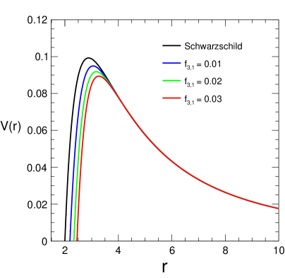
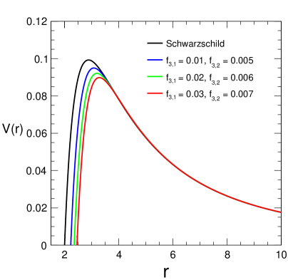
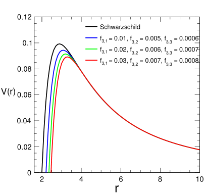
Figure 1: Behavior of black hole potential (29) with radial distance $r$ for different metric corrections obtained by considering the positive values of the coefficients $f_{3,n}$.

In Fig. 2 we plot $V(r)$ with respect to $r$ for negative values of the coefficients $f_{3,n}$. Here the left plot is for the 1st-order metric correction, the middle one is for up to 2nd-order metric corrections and the right one is for up to 3rd-order metric corrections. From Fig. 2 it is clear that the height of the peak of the potential increases with more negative values of the coefficients $f_{3,n}$. Moreover, it can also be observed that the height of the peak increases with the inclusion of higher order corrections to the metric. Further, in this case, the peak values of metric corrected potential are higher than the uncorrected Schwarzschild case. However, in this case also all potentials are merged together after a certain value of $r$ as in the previous case.

     

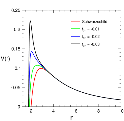
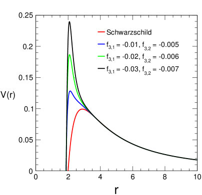
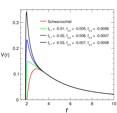
Figure 2: Behavior of black hole potential (29) with radial distance $r$ for different metric corrections obtained by considering the negative values of the coefficients $f_{3,n}$.

In Fig 3 we plot $V(r)$ with respect to $r$ with negative values of $f_{3,1}$ and positive values of $f_{3,2}$ for up to 2nd-order and 3rd-order metric corrections. Here the left plot is for up to 2nd-order metric corrections and the right plot is for up to 3rd-order metric corrections. In this case also the peak of the potential increases with the magnitude of the parameters $f_{3,n}$ and the height of the potential increases with the inclusion of higher order metric corrections. The rest of the behaviors are similar to the previous case.

   

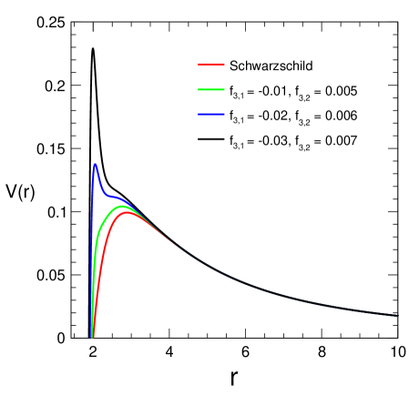
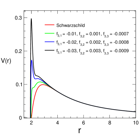
Figure 3: Variation of potential (29) with respect to $r$ for positive values of $f_{3,2}$. The left plot is for up to 2nd-order metric corrections and the right plot is for up to 3rd-order metric corrections.

We calculate the QNMs of the BH using the 6th-order Padé-averaged WKB approximation method in the form of their amplitude and damping, which is varying with respect to the coefficients $f_{3,1}$ and $f_{3,2}$. From Fig. 4 and Fig. 5 it can be observed that for both 1st-order and 2nd-order metric corrections, the general tendency of QNMs is that both amplitude and damping increases with the increasing magnitude of the coefficients $f_{3,1}$ and $f_{3,2}$ for all values of multiple $l$. In Fig. 4 we use the negative values of the coefficient $f_{3,1}$ and in Fig. 5 we keep $f_{3,1}=-\,0.01$ and consider the positive values of $f_{3,2}$. When we consider positive values of the coefficient $f_{3,1}$ it is found that the imaginary part of the QNMs becomes positive as shown in Table 3. The positive value of the imaginary or damping part of QNMs indicates the instability in the system as the perturbations increase with time. Further, when we consider negative values of the coefficients $f_{3,2}$, keeping $f_{3,1}$ negative and when we consider positive values for both $f_{3,1}$ and $f_{3,2}$, similar results are obtained.

   

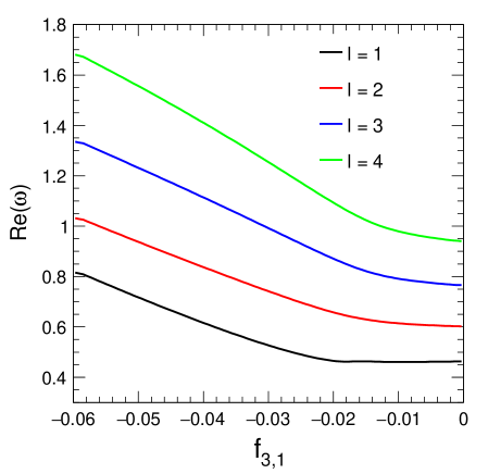
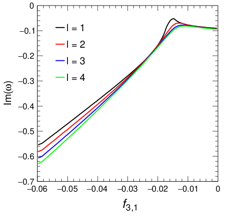
Figure 4: Variation of real and imaginary parts of QNMs with respect to negative values of $f_{3,1}$ for the 1st-order correction and for different values of $l$.

   

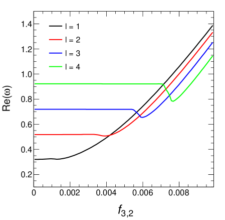
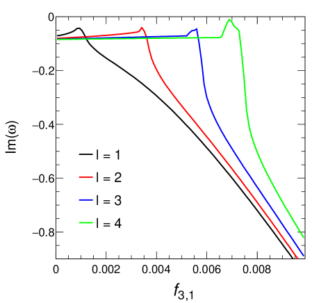
Figure 5: Variation of real and imaginary parts of QNMs with respect to $f_{3,2}$ for the 2nd-order correction and for different values of $l$. Here we consider $f_{3,1}=-\,0.01$.

The error associated with the WKB method of calculation of QNMs has been estimated using a well-established formula, commonly found in the literature, which is as follows [90, 91, 52]:

$$\Delta_{6}=\frac{|\text{WKB}_{7}-\text{WKB}_{5}|}{2},$$ (31)

where $\text{WKB}_{7}$ and $\text{WKB}_{5}$ are the 7th and 5th-order QNMs obtained from the Padé averaged WKB method respectively.

For more clarity in the behaviors QNMs of the BH for the scalar field perturbations with different orders of metric corrections as discussed in relation to Figs. 4 and 5, we list the corresponding values of QNMs together with the associated errors in Tables 1–5. Table 1 shows the QNMs of the BH with the corresponding calculated errors for the 1st-order metric correction and for negative values of the coefficients $f_{3,1}$ with three different values of multipole moment $l$. From this table, it can be observed that as seen in Fig. 4 both the oscillation and damping of the QNMs increase with the multipole moment and magnitude of $f_{3,1}$. It is also seen that the errors of the calculations of the QNMs are very small for smaller values of $l$, which increase with the increasing value of $l$ and are in general smaller than the uncorrected Schwarzschild case. Moreover, in general, the error decreases with the increasing magnitude of the coefficient $f_{3,1}$.

Table 1: 6th-order Padé averaged WKB QNMs of the BH defined by the metric (13) for the 1st-order correction, with multipoles $l=1,\,2,\,3$ and $n=0$. We use different negative values of the parameter $f_{3,1}$.

Multipole	$f_{3,1}$	Padé averaged 6th-order WKB	$\Delta_{6}$
Schwarzschild ($l=1$)	0	$0.292936-0.097660i$	$0.3140\times 10^{-5}$
$l=1$	$-0.012$	$0.461274-0.071067i$	$0.3187\times 10^{-6}$
	$-0.015$	$0.463277-0.050489i$	$0.7825\times 10^{-6}$
	$-0.018$	$0.461195-0.118660i$	$0.6511\times 10^{-5}$
	$-0.021$	$0.468746-0.174250i$	$0.3463\times 10^{-6}$
Schwarzschild ($l=2$)	0	$0.483647-0.096718i$	$0.5298\times 10^{-4}$
$l=2$	$-0.012$	$0.619113-0.071169i$	$0.2159\times 10^{-3}$
	$-0.015$	$0.629781-0.076175i$	$0.0710\times 10^{-5}$
	$-0.018$	$0.644586-0.126197i$	$0.0721\times 10^{-6}$
	$-0.021$	$0.664840-0.173427i$	$0.5194\times 10^{-6}$
Schwarzschild ($l=3$)	0	$0.599440-0.09270i$	$0.4719\times 10^{-3}$
$l=3$	$-0.012$	$0.800980-0.076887i$	$0.2513\times 10^{-3}$
	$-0.015$	$0.821367-0.092311i$	$0.3175\times 10^{-3}$
	$-0.018$	$0.849275-0.133391i$	$0.6540\times 10^{-3}$
	$-0.021$	$0.882445-0.176460i$	$0.1763\times 10^{-4}$

Table 2 shows the QNMs with the associated errors of calculations for the 2nd-order metric correction with positive values of $f_{3,2}$ while keeping $f_{3,1}=-\,0.01$ with the same values of $l$ as in the previous case. The results shown in this table are similar to that shown in Fig. 5. From this table, it can be clearly observed that in general, with an increase in $l$ and $f_{3,2}$ the oscillation and damping of the QNMs also increase. However, for higher values of $l$ difference of the values of the QNMs for increasing values of $f_{3,2}$ is very small up to a certain higher value of $f_{3,2}$, and such a small difference could not be observed in Fig. 5 due to the size of scale used to plot the QNMs. Although, in general, the errors of calculations of QNMs are samll, the error increases randomly without following a particular pattern due to the peculiar nature of the QNMs in this case as mentioned.

Table 2: 6th-order Padé averaged WKB QNMs of the BH defined by the metric (13) for the 2nd-order correction, with multipoles $l=1,\,2,\,3$ and $n=0$. We use different positive values of the parameter $f_{3,2}$ keeping $f_{3,1}=-\,0.01$.

Multipole	$f_{3,2}$	Padé averaged 6th-order WKB	$\Delta_{6}$
$l=1$	$0.001$	0.326565 - 0.030865i	$0.1732\times 10^{-3}$
	$0.003$	0.402747 - 0.217869i	$0.6154\times 10^{-6}$
	$0.005$	0.608456 - 0.385280i	$0.5710\times 10^{-6}$
	$0.007$	0.896927 - 0.598825i	$0.0571\times 10^{-4}$
	$0.008$	1.060840 - 0.721304i	$0.2162\times 10^{-6}$
$l=2$	$0.001$	0.517537 - 0.075501i	$0.0071\times 10^{-6}$
	$0.003$	0.518963 - 0.060009i	$1.7260\times 10^{-4}$
	$0.005$	0.570409 - 0.331340i	$1.7260\times 10^{-4}$
	$0.007$	0.835102 - 0.564314i	$3.5760\times 10^{-2}$
	$0.008$	1.002850 - 0.691294i	$0.6430\times 10^{-6}$
$l=3$	$0.001$	0.719024 - 0.080950i	$1.7220\times 10^{-6}$
	$0.003$	0.718888 - 0.076272i	$0.4220\times 10^{-3}$
	$0.005$	0.718777 - 0.071456i	$0.3210\times 10^{-6}$
	$0.007$	0.757422 - 0.489539i	$4.1200\times 10^{-3}$
	$0.008$	0.918746 - 0.634811i	$0.3724\times 10^{-6}$

Table 3 shows the QNMs for the 1st-order metric correction with positive values of the coefficient $f_{3,1}$. From this table, one can observe that for the positive value of the coefficients $f_{3,1}$ the imaginary part of the QNMs becomes positive. Further, it can be observed from this Table 3 that with an increase in $l$ and value of the coefficient $f_{3,1}$ the oscillation decreases. Moreover, the imaginary part decreases with the increasing value of the coefficient $f_{3,1}$. Table 4 and Table 5 show the QNMs of the BH for the 2nd-order metric correction. In Table 4 we keep $f_{3,1}=-\,0.01$ and consider the negative values of $f_{3,2}$ and in Table 5 we keep $f_{3,1}=0.01$ and consider the positive values of $f_{3,2}$. From both Tables 4 and 5 it can be observed that most of the QNMs have positive imaginary parts, and the oscillation increases with $l$ in Table 4, whereas it decreases with $l$ in Table 5 for the cases with the positive imaginary part. It can also be observed that with the higher value of correction to the metric the oscillation and imaginary part of the QNMs decrease. As mentioned above, the QNMs with positive imaginary parts indicate a physically unstable situation in a system. Thus the metric corrections that result in the QMNs with positive imaginary parts are not the desirable corrections to be considered for further analysis.

Table 3: 6th-order Padé averaged WKB QNMs of the BH defined by the metric (13) for the 1st-order correction, with multipoles $l=1,\,2,\,3$ and $n=0$. We use different positive values of the parameter $f_{3,1}$.

Multipole	$f_{3,1}$	Padé averaged 6th-order WKB	$\Delta_{6}$
$l=1$	$0.0009$	0.284557 + 0.233900i	$0.043\times 10^{-3}$
	$0.0012$	0.254602 + 0.213049i	$0.811\times 10^{-6}$
	$0.0015$	0.234694 + 0.198055i	$0.723\times 10^{-6}$
	$0.0018$	0.220560 + 0.186605i	$4.120\times 10^{-6}$
$l=2$	$0.0009$	0.195980 + 0.356975i	$0.512\times 10^{-6}$
	$0.0012$	0.166610 + 0.356975i	$1.280\times 10^{-3}$
	$0.0015$	0.148133 + 0.302626i	$0.432\times 10^{-6}$
	$0.0018$	0.135858 + 0.285388i	$0.072\times 10^{-6}$

Table 4: 6th-order Padé averaged WKB QNMs of the BH defined by the metric (13) for 2nd-order correction, with multiploles $l=1,\,2,\,3$ and $n=0$. We use different negative values of the parameter $f_{3,2}$ keeping $f_{3,1}=-\,0.01$.

Multipole	$f_{3,2}$	Padé averaged 6th-order WKB	$\Delta_{6}$
$l=1$	$-0.0009$	0.408285 + 0.0671545i	$0.351\times 10^{-6}$
	$-0.0012$	0.330561 + 0.0578801i	$0.072\times 10^{-4}$
	$-0.0015$	0.290344 + 0.0546129i	$0.081\times 10^{-6}$
	$-0.0018$	0.266919 + 0.0543525i	$3.210\times 10^{-6}$
$l=2$	$-0.0009$	0.673305 + 0.1415410i	$1.530\times 10^{-6}$
	$-0.0012$	0.548048 + 0.0936886i	$3.210\times 10^{-3}$
	$-0.0015$	0.480284 + 0.0936886i	$0.007\times 10^{-6}$
	$-0.0018$	0.439153 + 0.0801412i	$0.341\times 10^{-6}$

Table 5: 6th-order Padé averaged WKB QNMs of the BH defined by the metric (13) for 2nd-order correction, with multipoles $l=1,\,2,\,3$ and $n=0$. We use different positive values of the parameter $f_{3,2}$ keeping $f_{3,1}=0.01$.

Multipole	$f_{3,2}$	Padé averaged 6th-order WKB	$\Delta_{6}$
$l=1$	$0.0009$	0.150081 + 0.079249i	$0.241\times 10^{-5}$
	$0.0012$	0.146698 + 0.072319i	$0.117\times 10^{-6}$
	$0.0015$	0.140635 + 0.063404i	$0.351\times 10^{-3}$
	$0.0018$	2.032860 - 1.049390i	$0.007\times 10^{-6}$
$l=2$	$0.0009$	0.056441 + 0.179632i	$0.072\times 10^{-6}$
	$0.0012$	0.017200 + 0.021268i	$0.718\times 10^{-3}$
	$0.0015$	0.172300 + 0.250931i	$0.314\times 10^{-6}$
	$0.0018$	2.283400 - 1.099100i	$0.291\times 10^{-6}$

IV Evolution of a Scalar Perturbation Around the Black Hole

In this section, we study the evolution of a scalar perturbation around the BH spacetime for the 1st-order and 2nd-order corrections to the metric. To study the evolution of the scalar field perturbation we use the time domain integration method described in Refs. [92, 93]. Thus, defining $\Psi(r_{\star},t)=\Psi(i{\Delta}r_{\star},j{\Delta}t)=\Psi_{i,j}$ and $V(r(r_{\star}))=V(r_{\star},t)=V_{i,j}$, Eq. (24) can be expressed in the following form:

$$\frac{\Psi_{i+1,j}-2\Psi_{i,j}+\Psi_{i-1,j}}{{\Delta}r_{\star}^{2}}-\frac{\Psi_{i,j+1}-2\Psi_{i,j}+\Psi_{i,j-1}}{{\Delta}t^{2}}-V_{i}\Psi_{i,j}=0.$$ (32)

Now using the initial conditions: $\Psi(r_{\star},t)=\exp\left[-(r_{\star}-k)^{2}/2\lambda^{2}\right]$ and $\left|\Psi(r_{\star},t)\right|_{t<0}=0$, where $k$ is the median and $\lambda$ is the width of the initial wave packet, the final expression for the time evolution of the scalar field can be written as

$$\Psi_{i,j+1}=-\,\Psi_{i,j-1}+\left(\frac{{\Delta}t}{{\Delta}r_{\star}}\right)^{\!2}\left(\Psi_{i+1,j}+\Psi_{i-1,j}\right)+\left(2-2\left(\frac{{\Delta}t}{{\Delta}r_{\star}}\right)^{\!2}-V_{i\,}\Delta{t}^{2}\right)\Psi_{i,j}.$$ (33)

Moreover, we apply the Von Neumann stability condition: $\frac{{\Delta}t}{{\Delta}r_{\star}}<1$ during the numerical procedure to ensure stable results and compute the time profiles.

   

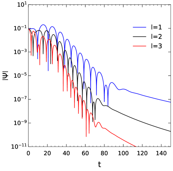
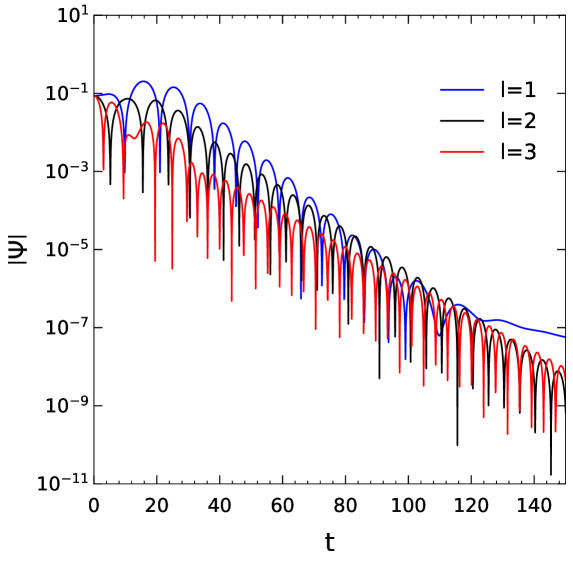
Figure 6: Time domain profiles for the scalar field perturbation around the BH spacetime defined by the metric (13). The left plot is for the 1st-order correction to metric with $f_{3,1}=-\,0.02$ and the right plot is for the 2nd-order correction to the metric with $f_{3,1}=-\,0.01$ and $f_{3,2}=0.005$.

   

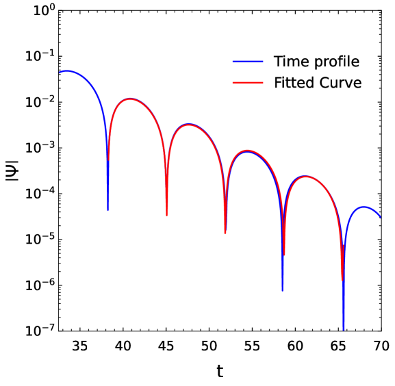
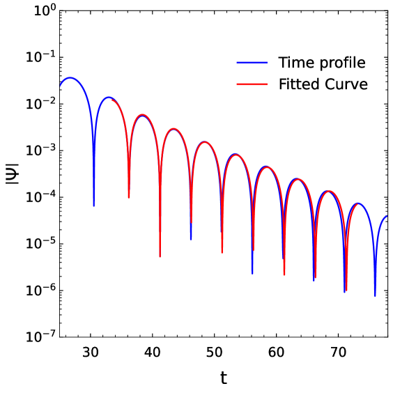
Figure 7: Estimation of QNMs by fitting the time domain profile using the Levenberg Marquardt algorithm [94, 95, 96]. In the left plot, we fit the time domain profiles obtained from the 1st-order metric correction considering $l=1$ and $f_{3,1}=-\,0.02$. In the right plot, we fit the time domain profile obtained from the 2nd-order metric correction considering $l=2$, $f_{3,1}=-\,0.01$ and $f_{3,2}=0.005$.

In Fig. 6 we plot the time domain profiles obtained from the 1st-order and 2nd-order metric corrections. From Fig. 6 it can be observed that the time domain profile varies with multiple moment $l$, showing a good agreement with the results obtained from the Padé averaged WKB approximation method. Further, we employ the Levenberg Marquardt algorithm [94, 95, 96] to estimate the QNMs from the time domain profiles. Fig. 7 demonstrates the estimation of QNMs by fitting the time domain profiles. In the left plot of this figure, we fit the time domain profile obtained from the 1st-order metric correction considering $f_{3,1}=-\,0.02$, and we obtain the QNM as $0.4657909598-0.154704584i$. In the right plot, we fit the time domain profile obtained from the 2nd-order metric correction considering $f_{3,1}=-\,0.02$ and $f_{3,2}=0.005$, and we obtain the QNM as $0.6053625411-0.383951357i$. Additionally, we determine the difference in the magnitudes of the QNMs obtained from the 6th-order Padé averaged WKB approximation method and those obtained using the time domain analysis method as follows:

$$\Delta_{\text{QNM}}=\frac{\left|\text{QNM}_{\text{WKB}}-\text{QNM}_{\text{Time domain}}\right|}{2}.$$ (34)

Table 6: Comparison of QNMs obtained from the time domain profiles and Padé averaged WKB method for the 1st-order metric correction considering $f_{3,1}=-\,0.02$.

l	Time domain	$R^{2}$	Padé averaged WKB	$\Delta_{\text{QNM}}$
$l=1$	$0.465790960-0.154704584i$	$0.975360$	$0.465088-0.158462i$	$0.000265$
$l=2$	$0.651392510-0.155052142i$	$0.977538$	$0.657593-0.158505i$	$0.003410$
$l=3$	$0.871569312-0.165721320i$	$0.968405$	$0.870989-0.162352i$	$0.003420$

Table 7: Comparison of QNMs obtained from the time domain profiles and Padé averaged WKB method for the 2nd-order metric correction considering $f_{3,1}=-\,0.01$ and $f_{3,2}=0.005$.

l	Time domain	$R^{2}$	Padé averaged WKB	$\Delta_{\text{QNM}}$
$l=1$	$0.60315541-0.38217522i$	$0.95890551$	$0.607196-0.384308i$	$0.004570$
$l=2$	$0.57102810-0.33217638i$	$0.97922510$	$0.570424-0.331178i$	$0.001170$
$l=3$	$0.71953215-0.06992590i$	$0.96897990$	$0.718777-0.071480i$	$0.001730$

Table 6 shows the QNMs obtained from the time domain profiles along with QNMs obtained from the Padé averaged WKB approximation method for $l=1$, $2$ and $3$ considering the 1st-order metric correction. Similarly, Table 7 shows the QNMs obtained from the time domain profiles along with QNMs obtained from the Padé averaged WKB approximation method for $l=1$, $2$ and $3$ considering the 2nd-order metric correction. In both the tables we show the $R^{2}$ value of the fitting. From the time domain analysis, it can be observed that for both 1st-order and 2nd-order metric corrections oscillation as well as decay of QNMs increases with multipole $l$. Further, it can be also observed that the results obtained from the time domain analysis are in good agreement with the results obtained from the Padé averaged WKB approximation method.

V Shadow of the black hole

The study of BH shadow provides an opportunity to test different theories of gravity as well as helps in the study of gravity in the BH’s extreme gravity regimes. The shape of the shadow formed by a BH is determined by the parameters of the underlying theory and is defined by the photon sphere. The photon sphere is a region around the BH where gravity is so strong that photons, or light particles, travel in unstable circular orbits around the BH. In this section, our aim is to study the behavior of the shadow when higher-order corrections of the IDG are included and for different values of the free model parameters.

For a system with spherically symmetric and static spacetime metric the Lagrangian $\mathcal{L}(x,\dot{x})$ of that system can be expressed as [51]

$$\mathcal{L}(x,\dot{x})\equiv\frac{1}{2}g_{\mu\nu}\dot{x}^{\mu}\dot{x}^{\nu}=\frac{1}{2}\Big{[}-f(r)\,\dot{t}^{2}+\frac{1}{g(r)}\,\dot{r}^{2}+r^{2}(\dot{\theta}^{2}+Sin^{2}\theta\dot{\phi}^{2})\Big{]},$$ (35)

where the dots over the variables represent differentiation with respect to the proper time $\tau$. For our considered BH system the metric functions $f(r)$ and $g(r)$ are given respectively by Eqs. (14) and (15). Now, the null geodesic equation for photons is [51]

$$-f(r)\,\dot{t}^{2}+\frac{1}{g(r)}\,\dot{r}^{2}+r^{2}\dot{\phi}^{2}=0.$$ (36)

By utilizing the Euler-Lagrange equation

$$\frac{d}{d\tau}\left(\frac{\partial\mathcal{L}}{\partial\dot{x}^{\mu}}\right)-\frac{\partial\mathcal{L}}{\partial x^{\mu}}=0$$

we can obtain two conserved quantities of the system, viz. energy $\mathcal{E}$ and angular momentum $L$ which are given by $\mathcal{E}=f(r)\,\dot{t}$ and $L=r^{2}\,\dot{\phi}$. Using these two conserved quantities in Eq. (36) the reduced potential for the photons’ orbital motion can be obtained as [51, 97]

$$U_{r}=\frac{{L^{2}}{g(r)}}{r^{2}}.$$ (37)

Since angular momentum $L$ is a conserved quantity, the behaviour of the reduced potential will not depend on it, so we will consider $L=1$ in our further calculations.

     

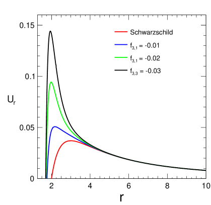
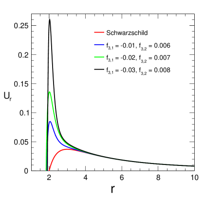
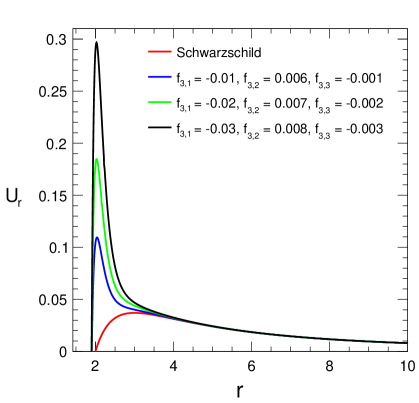
Figure 8: Variation of reduced potential $U_{r}$ given by Eq. (37) with radial distance $r$ for different metric corrections and for different values of the free parameters.

Fig. 8 shows the variation of the reduced potential $U_{r}$ with respect to $r$. In the left plot of this figure, we show $U_{r}$ variation with respect to $r$ for the 1st-order metric correction. In the middle plot we show the same for up to the 2nd-order metric corrections and in the right plot we show it for up to the 3rd-order metric corrections. From Fig 8 it is observed that for 1st-order metric correction with the increase of the negative values of $f_{3,1}$ the peak of the reduce potential increases, for the 2nd-order metric corrections with the increase positive values of $f_{3,2}$ while keeping $f_{3,1}$ negative with increasing magnitude the peak of the potential increases and for the 3rd-order metric corrections keeping $f_{3,1}$ negative and $f_{3,2}$ positive with negative values of $f_{3,3}$ the peak of the potential also increases for increasing magnitudes of all these coefficients. Moreover, similar to the potential (29), in this case also the peak of the potential increases substantially with increasing order of corrections and the corrected potential peak is significantly higher than the Schwarzschild case. Further, all potential values merged together after a certain value of $r$ depending on the order of corrections. Since from the QNMs study we observed that for other sign combinations of the parameters the BH system becomes unstable, here we consider the stable cases only.

Now we move to study the shadow radius. To study the shadow radius one needs to first determine the radius of the photon sphere. The photon sphere radius can be obtained by solving the following equation [51, 98, 99]:

$$\left.\frac{f^{\prime}(r)}{f(r)}\right|_{r\,=\,r_{\text{ph}}}=\left.\frac{h^{\prime}(r)}{h(r)}\right|_{r\,=\,r_{\text{ph}}},$$ (38)

where $r_{ph}$ represents the radius of the photon sphere and $h(r)=r^{2}$. This equation leads to the shadow radius $R_{s}$ for a static observer at a large distance as

$$R_{s}=\frac{r_{ph}}{\sqrt{f(r_{ph})}}.$$ (39)

The stereographic projection of the BH’s shadow from the plane of the black hole to the observer’s observation plane using coordinates $(X,Y)$ can be used to determine the shadow’s apparent shape. The coordinates $(X,Y)$ is defined as [100]

$$X =\lim_{r_{0}\to\infty}\left(-\,r_{0}^{2}\sin\theta_{0}\,\frac{d\phi}{dr}\Big{|}_{r_{0}}\right),$$ (40)

$$Y =\lim_{r_{0}\to\infty}\left(r_{0}^{2}\,\frac{d\theta}{dr}\Big{|}_{(r_{0},\theta_{0})}\right),$$ (41)

where $r_{0}$ is the position of the observer and $\theta_{0}$ is the angular position of the observer with respect to the BH plane.

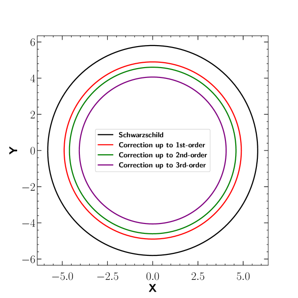
Figure 9: Stereographic mapping of the variation of shadow radius in celestial coordinates for the addition of different orders of metric corrections.

   

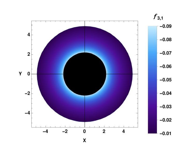
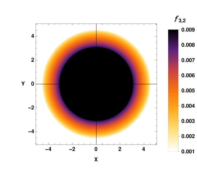
Figure 10: Stereographic mapping of the variation of shadow radius in celestial coordinates. The left plot shows the variation of shadow radius with the 1st-order correction coefficient $f_{3,1}$ and the right plot shows the variation of the same with the 2nd-order correction coefficient $f_{3,2}$ considering $f_{3,1}=-\,0.01$.

Fig. 9 shows the stereographic mapping of the variation of the shadow radius with the inclusion of different orders of metric corrections. From the figure one can observe that with the inclusion of higher order corrections to the metric, the radius of the shadow decreases. Fig. 10 shows the stereoscopic mapping of the variation of the shadow radius with respect to the free parameters $f_{3,1}$ and $f_{3,2}$. In the left plot of this figure we show the variation of the shadow radius with negative values of $f_{3,1}$ and in the right plot show the variation of the shadow radius with positive values of $f_{3,2}$. It can be observed from Fig. 10 also that the shadow radius decreases as the magnitudes of $f_{3,1}$ and $f_{3,2}$ increases.

To constrain the coefficients $f_{3,1}$ and $f_{3,2}$, we utilize the technique described in Ref. [101]. It is to be noted that due to the complexity of the process we could not include the coefficient $f_{3,3}$ for the constraining. Here, we outline some key steps of this approach. The main idea is to compare the observed angular radius of the Sgr A* BH, which was recently measured by the EHT collaboration with the theoretically computed shadow radius from Eq. (39). This comparison helps us impose constraints on the model parameters. It is important to have a prior value for the mass-to-distance ratio of the Sgr A*. Another crucial aspect of this method is the calibration factor, which connects the observed shadow radius to the theoretical prediction. Similar methods have been used in previous studies [102, 103, 104] and we will follow the same strategy in this regard. The EHT group introduced a new parameter $\delta$, which represents the fractional deviation between the observed shadow radius $R_{s}$ and the shadow radius of a Schwarzschild BH $R_{sch}$. Thus the parameter $\delta$ can be defined as follows [101]:

$$\delta=\frac{R_{s}}{R_{sch}}-1=\frac{R_{s}}{3{\sqrt{3}}M}-1.$$ (42)

The estimated values of the parameter $\delta$ from the measurements of Keck and VLTI experiments are [101] $\delta=-\,0.04^{+0.09}_{-0.10}$ (Keck) and $\delta=-\,0.08^{+0.09}_{-0.09}$ (VLTI) respectively. For simplicity, we consider the mean of these two observational values as in the case of Ref. [101]. The mean value of $\delta$ is

$$\delta=-\,0.060\pm 0.065.$$ (43)

As mentioned in Ref. [101], considering a Gaussian distribution of $\delta$ with $\sigma=0.065$ as the standard deviation, calculated the $1\sigma$ and $2\sigma$ intervals for the $\delta$ parameter as

$$-\,0.125 \lesssim\delta\lesssim 0.005\quad(1\sigma),$$ (44)

$$-\,0.190 \lesssim\delta\lesssim 0.070\quad(2\sigma).$$ (45)

These bounds for $\delta$ in Eq. (44) and Eq. (45) when used in Eq. (42), give the bounds on the Schwarzschild radius $R_{sch}$ as

$$4.55 \lesssim\frac{r_{sh}}{M}\lesssim 5.22\quad(1\sigma),$$ (46)

$$4.21 \lesssim\frac{r_{sh}}{M}\lesssim 5.56\quad(2\sigma).$$ (47)

In Fig. 11 we plot the shadow radius with respect to coefficients $f_{3,1}$ and $f_{3,2}$, with the bounds imposed by the observations of Keck and VLTI experiments. In the plots of this figure, the light yellow regions are forbidden zones, the blue regions are allowed zones by $2\sigma$ bound and the violet regions are allowed zones by $1\sigma$ bound. In the left plot, we draw $R_{s}$ with respect to $f_{3,1}$. It can be observed from this plot that for more negative values of $f_{3,1}$ the shadow radius rapidly moves to the forbidden region, whereas with less negative values of $f_{3,1}$ the shadow radius goes into the allowed region. In the right plot, we show the $R_{s}$ variation with respect to $f_{3,2}$. We can observe from this plot that as the value of $f_{3,2}$ increases, the shadow radius quickly moves to the forbidden region, while for less positive values of $f_{3,2}$ the shadow radius falls in the allowed $2\sigma$ and $1\sigma$ region depending on the value of $f_{3,1}$. More negative values of $f_{3,1}$ push $R_{s}$ out of the allowed region for more early positive values of $f_{3,2}$ than otherwise.

This approach to constraining theoretical parameters has been utilized in the literature [102, 103] and by the EHT collaboration [101], offering a reliable method for parameter estimation. However, when dealing with multiple model parameters, additional complementary techniques are required to isolate individual parameters and achieve more stringent constraints. We leave this aspect for future exploration.

   

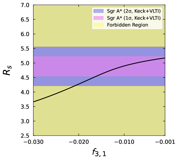
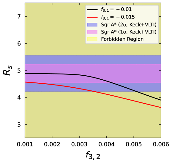
Figure 11: Shadow radius versus the coefficients $f_{3,1}$ and $f_{3,2}$ in the background of Keck and VLTI experiments’ constrains [101] obtained from the observations of Sgr $A^{*}$. The yellow portions represent the zone forbidden by the Keck-VLTI observations.

VI Summery and Conclusion

The primary goal of this study is to investigate how different corrections to the Schwarzschild metric alter the BH’s observables. We also studied the effects of the variation of free parameters on BH’s observables. In this direction, we studied the effects on BH’s QNMs and the BH’s shadow that are introduced by the metric corrections up to 2nd-order terms. The study up to 2nd-order metric correction can provide us valuable information about the low energy QG effects.

In Section III we studied the QNMs of the BH. Figs. 1, 2 and 3 show the behavior of the BH’s effective potential with respect to $r$ for different corrections to the metric and for different values of the free parameters. It is seen that the peak of the effective potential decreases compared to the Schwarzschild case for the positive values of the metric correction coefficients $f_{3,1}$, $f_{3,2}$ and $f_{3,3}$, and the height of the peak remains same even after the inclusion of higher-order corrections. However, for the negative values of these parameters, the peak of the effective potential is higher compared to the Schwarzschild case and as the parameters become more negative the peak increases, which increases further with the inclusion of the higher-order corrections. Further, for negative values of $f_{3,1}$, positive values of $f_{3,2}$ and negative values of $f_{3,3}$, it was also found that the peak of the effective potential increases compared to Schwarzschild case as the values of the free parameters increase. In this case also the peak of the effective potential increases with the inclusion of higher-order corrections. Moreover, all potential values merged together after a certain value of $r$ depending on the order of corrections. Thus we can say that the sign and magnitude of these parameters play an important role in the behavior of the effective potential $V(r)$. We calculated the QNMs of the BH using the 6th-order Padé-averaged WKB approximation method. Figs. 4 and 5 show the behavior of the real and imaginary parts of the QNMs with respect to the correction parameters up to the 2nd-order. The calculated values of QNMs were presented in Tables 1–5 for different sign combinations of the parameters. From these tables, it is clear that QNMs have negative imaginary parts when the values of $f_{3,1}$ are negative for 1st-order metric correction. This is also the case for the metric corrections up to 2nd-order when the values of $f_{3,1}$ are negative and $f_{3,2}$ are positive. Whereas, for all other sign combinations of $f_{3,1}$ and $f_{3,2}$ the imaginary parts of the QNMs become positive. As the positive imaginary part indicates instability in the BH system, we considered only the cases where $f_{3,1}$ is negative and $f_{3,2}$ is positive in further analysis of this study.

In Section IV we studied the evolution of a scalar field perturbation around our considered BH. It is clearly visible from the time profile that the oscillation and decay of QNMs are in agreement with the results that are obtained from the 6th-order Padé-averaged WKB approximation method. We also calculated the QNMs from the time profile of the evolution using the Levenberg-Marquardt algorithm. It can be seen that the QNM frequencies are almost equal for both methods used. Further, the discrepancy between the results of these two methods is quantified using the parameter $\Delta_{\text{QNM}}$, defined in Eq. (34).

In Section V we studied the shadow of the BH. Fig. 8 shows the behavior of the reduced potential $U_{r}$ with respect to $r$ for different values of the free parameters and for different corrections. It can be observed that the peak of the reduced potential increases with the magnitudes of the correction parameters and also with the inclusion of higher-order corrections. Further, we showed the Stereographic mapping of the shadow radius. It can be seen from Fig. 9 that the radius of the shadow decreases with the inclusion of higher-order corrections to the metric. We also showed the variation of the shadow radius with respect to $f_{3,1}$ and $f_{3,2}$. It was found that for the correction up to 1st-order the shadow radius decreases with negative values of $f_{3,1}$ and for the corrections up to 2nd-order shadow radius decreases with positive values of $f_{3,2}$ while keeping $f_{3,1}$ negative. Further, we constrained $f_{3,1}$ and $f_{3,2}$ using the data from the Keck and VLTI observations.

As mentioned already, our study mainly focused on how the corrections to the metric can make changes to the BH’s observables, viz. QNMs and shadow, and how the observables behave with respect to the parameters of the theory. To study the effects arising from the metric corrections we consider up to the 2nd-order corrections for simplicity. The more higher-order corrections will create more mathematical complexity. However, the corrections to the Schwarzschild metric up to 2nd-order introduced by the IDG have provided a significant deviation to the BH’s QNMs and shadow radius from the results that are obtained from GR. We hope this study will contribute towards a better understanding of the effects on BH’s observables arising from the higher-order correction to the metric in the IDG. This study also sheds light on our understanding of low-energy QG effects and offers valuable insights for future research.

References

- [1] B. P. Abbott et al., Observation of Gravitational Waves from a Binary Black Hole Merger, Phys. Rev. Lett. 116, 061102 (2016).
- [2] B. P. Abbott et al., GW151226: Observation of Gravitational Waves from a 22-Solar-Mass Binary Black Hole Coalescence, Phys. Rev. Lett. 116, 241103 (2016).
- [3] B. P. Abbott et al., GW170817: Observation of Gravitational Waves from a Binary Neutron Star Inspiral, Phys. Rev. Lett. 119, 161101 (2017).
- [4] R. Abbott et al., GW190412: Observation of a Binary-Black-Hole Coalescence with Asymmetric Masses, Phys. Rev. D 102, 043015 (2020).
- [5] R. Abbott et al., Observation of Gravitational Waves from Two Neutron Star–Black Hole Coalescences, Astrophys. J. Lett. 915, L5 (2021).
- [6] The Event Horizon Telescope Collaboration, First M87 Event Horizon Telescope Results. IV. Imaging the Central Supermassive Black Hole, Astrophys. J. Lett. 875, L4 (2019).
- [7] The Event Horizon Telescope Collaboration, First M87 Event Horizon Telescope Results. II. Array and Instrumentation, Astrophys. J. Lett. 875, L2 (2019).
- [8] The Event Horizon Telescope Collaboration, First M87 Event Horizon Telescope Results. III. Data Processing and Calibration, Astrophys. J. Lett. 875, L3 (2019).
- [9] The Event Horizon Telescope Collaboration, First M87 Event Horizon Telescope Results and the Role of ALMA, The Messenger 177, 25 (2019).
- [10] The Event Horizon Telescope Collaboration, First M87 Event Horizon Telescope Results. V. Physical Origin of the Asymmetric Ring, Astrophys. J. Lett. 875, L5 (2019).
- [11] The Event Horizon Telescope Collaboration, First M87 Event Horizon Telescope Results. VI. The Shadow and Mass of the Central Black Hole, Astrophys. J. Lett. 875, L6 (2019).
- [12] A. G. Riess et al., Observational evidence from supernovae for an accelerating universe and a cosmological constant, Astron. J. 116, 1009 (1998).
- [13] S. Perlmutter et al., Measurements of and from 42 High Redshift Supernovae, Astrophys. J. 517, 565 (1999).
- [14] C. Pérez de los Heros, Status, Challenges and Directions in Indirect Dark Matter Searches, Symmetry 12, 1648 (2020).
- [15] N. A. Bahcall et al., The Cosmic Triangle: Assessing the State of the Universe, Science 284, 1481 (1999).
- [16] G. Amelino-Camelia, Are we at the dawn of quantum gravity phenomenology?, Lect. Notes Phys. 541, 1 (2000).
- [17] R. Gambini et al., Fundamental decoherence from quantum gravity: A Pedagogical review, Gen. Rel. Grav. 39, 1143 (2007).
- [18] S. De et al., Quantum gravity as an emergent phenomenon, Int. J. Mod. Phys. D 28, 1944003 (2019).
- [19] M. Van Raamsdonk, Lectures on gravity and entanglement, Theor. Adv. Study Inst. Elem. Part. Phys. 5, 297 (2017).
- [20] R. Loll, Quantum Gravity from Causal Dynamical Triangulations: A Review, Class. Quant. Grav. 37, 013002 (2020).
- [21] A. Eichhorn, Asymptotically safe gravity, arXiv:2003.00044.
- [22] A. Ashtekar and E. Bianchi, A short review of loop quantum gravity, Rept. Prog. Phys. 84, 042001 (2021).
- [23] C. Rovelli, Loop quantum gravity, Living Rev. Rel. 1, 1 (1998).
- [24] H. Sahlmann, Loop Quantum Gravity - A Short Review, arXiv:1001.4188 [gr-qc].
- [25] F. Girelli, F. Hinterleitner, and S. Major, Loop Quantum Gravity Phenomenology: Linking Loops to Observational Physics, SIGMA 8, 098 (2012).
- [26] J. L. F. Barbon, String theory, Eur. Phys. J. C 33, S67 (2004).
- [27] E. T. Akhmedov, Review of modern string theory, Phys. Atom. Nucl. 72, 1574 (2009).
- [28] S. B. Giddings, Is string theory a theory of quantum gravity?, Found. Phys. 43, 115 (2013).
- [29] J. Maharana, Quantum gravity and string theory, 18th Conference of the Indian Association for General Relativity and Gravitation, 155 (1996).
- [30] J. Bedford, An Introduction to String Theory, arXiv:1107.3967 [hep-th].
- [31] J. F. Donoghue, General relativity as an effective field theory: The leading quantum corrections, Phys. Rev. D 50, 3874 (1994).
- [32] J. F. Donoghue, Introduction to the effective field theory description of gravity, arXiv:gr-qc/9512024.
- [33] S. Faller, Effective field theory of gravity: Leading quantum gravitational corrections to Newton’s and Coulomb’s law, Phys. Rev. D 77, 124039 (2008).
- [34] L. I. Bevilaqua, A. C. Lehum, and A. J. da Silva, Effective field theory of quantum gravity coupled to scalar electrodynamics, Class. Quant. Grav. 33, 095008 (2016).
- [35] D. Wallace, Quantum Gravity at Low Energies, arXiv:2112.12235 [gr-qc].
- [36] J. F. Donoghue and B. R. Holstein, Low Energy Theorems of Quantum Gravity from Effective Field Theory, J. Phys. G 42, 103102 (2015).
- [37] V. Cardoso et al., Black holes in an effective field theory extension of general relativity, Phys. Rev. Lett. 131, 109903 (2018).
- [38] S. Hollands, A. Ishibashi, and H. S. Reall, A stationary black hole must be axisymmetric in effective field theory, Commun. Math. Phys. 401, 2757 (2023).
- [39] S. Bhattacharyya, P. Biswas, A. Dinda, and N. Kundu, The zeroth law of black hole thermodynamics in arbitrary higher derivative theories of gravity, JHEP 2022, 13 (2022).
- [40] S. Bhattacharyya et al., An entropy current and the second law in higher derivative theories of gravity, JHEP 2021, 169 (2021).
- [41] I. Davies and H. S. Reall, Dynamical black hole entropy in effective field theory, JHEP 2023, 006 (2023).
- [42] S. Bhattacharjee, S. Sarkar, and A. C. Wall, Holographic entropy increases in quadratic curvature gravity, Phys. Rev. D 92, 064006 (2015).
- [43] F. Serra, Black Holes through the Lenses of Effective Field Theory, PhD thesis, Scuola Normale Superiore, Pisa, Italy (2023).
- [44] D. Wu, W. Liu, and J. Wang, Light rings and shadows of static black holes in effective quantum gravity, Phys. Lett. B 858, 139052 (2024).
- [45] I. Davies and H. S. Reall, Nonperturbative second law of black hole mechanics in effective field theory, Phys. Rev. Lett. 132, 171402 (2024).
- [46] R. Durrer, The cosmic microwave background: the history of its experimental investigation and its significance for cosmology, Class. Quant. Grav. 32, 124007 (2015).
- [47] P. Lemos and P. Shah, The Cosmic Microwave Background and , arXiv:2307.13083 [astro-ph.CO].
- [48] T. Biswas et al., Towards Singularity- and Ghost-Free Theories of Gravity, Phys. Rev. Lett. 108, 031101 (2012).
- [49] T. Biswas et al., Generalized ghost-free quadratic curvature gravity, Class. Quantum Grav. 31, 159501 (2014).
- [50] E. Witten, Noncommutative Geometry and String Field Theory, Nucl. Phys. B 268, 253 (1986).
- [51] R. Karmakar, D. J. Gogoi, and U. D. Goswami, Thermodynamics and shadows of GUP-corrected black holes with topological defects in Bumblebee gravity, Phys. Dark Univ. 41, 101249 (2023).
- [52] R. Karmakar and U. D. Goswami, Quasinormal modes, thermodynamics and shadow of black holes in Hu–Sawicki gravity theory, Eur. Phys. J. C 84, 969 (2024).
- [53] R. M. Wald, The thermodynamics of black holes, Living Rev. Rel. 4, 6 (2001).
- [54] B. Hazarika and P. Phukon, Thermodynamic topology of Horava Lifshitz black hole in two ensembles, Nucl. Phys. B 1006, 116649 (2024).
- [55] B. Hazarika, A. Bhattacharjee, and P. Phukon, Thermodynamics of rotating AdS black holes in Kaniadakis statistics, Annals Phys. 476, 169978 (2025).
- [56] R. Karmakar, D. J. Gogoi, and U. D. Goswami, Quasinormal modes and thermodynamic properties of GUP-corrected Schwarzschild black hole surrounded by quintessence, Int. J. Mod. Phys. A 37, 2250180 (2022).
- [57] D. Mondal, T. Roy, and U. Debnath, Thermodynamics of Euler-Heisenberg AdS black hole surrounded by quintessence field using shadow, Nucl. Phys. B 1014, 116859 (2025).
- [58] E. Elizalde, S. Nojiri, and S. D. Odintsov, Black Hole Thermodynamics and Generalised Non-Extensive Entropy, Universe 11, 60 (2025).
- [59] A. Baruah and P. Phukon, Restricted Phase Space Thermodynamics of 4D Dyonic AdS Black Holes: Insights from Kaniadakis Statistics and Emergence of Superfluid -Phase Transition, arXiv:2412.04375 (2024).
- [60] J. M. Maldacena, The Large limit of superconformal field theories and supergravity, Adv. Theor. Math. Phys. 2, 231 (1998).
- [61] D. T. Son and A. O. Starinets, Minkowski space correlators in AdS / CFT correspondence: Recipe and applications, JHEP 9, 042 (2002).
- [62] D. J. Gogoi and U. D. Goswami, Quasinormal modes of black holes with non-linear-electrodynamic sources in Rastall gravity, Phys. Dark Univ. 33, 100860 (2021).
- [63] F. Hosseinifar et al., Quasinormal Modes and Topological Characteristics of a Schwarzschild Black Hole Surrounded by the Dehnen Type Dark Matter Halo, arXiv:2503.03260 [gr-qc] (2025).
- [64] R. A. Konoplya and O. S. Stashko, Transition from Regular Black Holes to Wormholes in Covariant Effective Quantum Gravity: Scattering, Quasinormal Modes, and Hawking Radiation, arXiv:2502.05689.
- [65] G. Guo et al., Quasinormal modes of black holes with multiple photon spheres, JHEP 2022, 60 (2022).
- [66] R. Karmakar and U. D. Goswami, Quasinormal modes, temperatures and greybody factors of black holes in a generalized Rastall gravity theory, Phys. Scripta 99, 055003 (2024).
- [67] G. Mohan et al., Strong Lensing Effect and Quasinormal Modes of Oscillations of Black Holes in Gravity Theory, arXiv:2503.08402 [gr-qc] (2025).
- [68] R. A. Konoplya and A. Zhidenko, Quasinormal modes of black holes: From astrophysics to string theory, Rev. Mod. Phys. 83, 793 (2011).
- [69] G. Franciolini et al., Effective Field Theory of Black Hole Quasinormal Modes in Scalar-Tensor Theories, JHEP 2, 127 (2019).
- [70] F. S. Miguel, EFT corrections to scalar and vector quasinormal modes of rapidly rotating black holes, Phys. Rev. D 109, 104016 (2024).
- [71] D. M. Gingrich, Quasinormal modes of loop quantum black holes near the Planck scale, Phys. Rev. D 109, 044044 (2024).
- [72] H.-X. Jiang et al., Shadows of loop quantum black holes: semi-analytical simulations of loop quantum gravity effects on Sagittarius A* and M87*, JCAP 2024, 59 (2024).
- [73] S. Luo and C. Li, Black hole shadow of quantum Oppenheimer-Snyder–de Sitter spacetime, Phys. Rev. D 110, 124042 (2024).
- [74] S. Devi et al., Shadow of quantum extended Kruskal black hole and its super-radiance property, Phys. Dark Univ. 39, 101173 (2023).
- [75] J. L. Petersen, Introduction to the Maldacena conjecture on AdS / CFT, Int. J. Mod. Phys. A 14, 3597 (1999).
- [76] X.-Y. Hu, K.-J. He, and X.-X. Zeng, Holographic image features of an AdS black hole in Einstein-power-Yang-Mills gravity, arXiv:2406.03083 [hep-th].
- [77] J. Chen and J. Yang, Shadows and optical appearance of quantum-corrected black holes illuminated by static thin accretions, arXiv:2503.06215 [gr-qc].
- [78] N. Heidari et al., Absorption, scattering, geodesics, shadows and lensing phenomena of black holes in effective quantum gravity, Phys. Dark Univ. 47, 101815 (2025).
- [79] B. Hazarika and P. Phukon, Thermodynamic Properties and Shadows of Black Holes in Gravity, Front. Phys. 20, 035201 (2025).
- [80] S. Nojiri and S. D. Odintsov, Black holes and their shadows in F(R) gravity, arXiv:2412.13775 [gr-qc].
- [81] N. Askour et al., On M87* and SgrA* observational constraints of Dunkl black holes, JHEP 46, 100349 (2025).
- [82] L. Balart, G. Panotopoulos, and Á. Rincón, On new regular charged black hole solutions: Limiting Curvature Condition, Quasinormal modes and Shadows, Annals Phys. 473, 169865 (2025).
- [83] N. Askour et al., Particle dynamics, black hole shadow and weak gravitational lensing in the f(Q) theory of gravity, Commun. Theor. Phys. 75, 125404 (2023).
- [84] Y. Xiao, Y. Chen, H. Feng, and C. Zhu, Black hole solutions and thermodynamics in the infinite derivative theory of gravity, Phys. Rev. D 103, 044064 (2021).
- [85] R. Karmakar, D. J. Gogoi, and U. D. Goswami, Thermodynamics and shadows of GUP-corrected black holes with topological defects in Bumblebee gravity, Phys. Dark Univ. 41, 101249 (2023).
- [86] T. Bronzwaer and H. Falcke, The Nature of Black Hole Shadows, Astrophys. J. 920, 155 (2021).
- [87] T. Biswas and S. Talaganis, String-Inspired Infinite-Derivative Theories of Gravity: A Brief Overview, Mod. Phys. Lett. A 30, 1540009 (2015).
- [88] J. Edholm, Infinite Derivative Gravity: A finite number of predictions, Ph.D. thesis, University of Lancaster. (2019).
- [89] R. A. Konoplya, Quasinormal modes in higher-derivative gravity: Testing the black hole parametrization and sensitivity of overtones, Phys. Rev. D 107, 064039 (2023).
- [90] D. J. Gogoi, R. Karmakar, and U. D. Goswami, Quasinormal modes of nonlinearly charged black holes surrounded by a cloud of strings in Rastall gravity, Int. J. Geom. Methods Mod. Phys. 20, 2350007 (2023).
- [91] R. A. Konoplya, Quasinormal behavior of the D-dimensional Schwarzschild black hole and the higher order WKB approach, Phys. Rev. D 68, 024018 (2003).
- [92] D. J. Gogoi and U. D. Goswami, Quasinormal Modes and Hawking Radiation Sparsity of GUP corrected Black Holes in Bumblebee Gravity with Topological Defects, J. Cosmol. Astropart. Phys. 2022, 29 (2022).
- [93] C. Gundlach, R. H. Price, and J. Pullin, Late-time behavior of stellar collapse and explosions. II. Nonlinear evolution, Phys. Rev. D 49, 890 (1994).
- [94] K. Levenberg, A Method for the Solution of Certain Non-Linear Problems in Least Squares, Quart. Appl. Math. 2, 164 (1944).
- [95] D. W. Marquardt, An Algorithm for Least-Squares Estimation of Nonlinear Parameters, SIAM J. Appl. Math. 11, 431 (1963).
- [96] E. Berti et al., Mining Information from Binary Black Hole Mergers: A Comparison of Estimation Methods for Complex Exponentials in Noise, Phys. Rev. D 75, 124017 (2007).
- [97] İ. Çimdiker, D. Demir, and A. Övgün, Black hole shadow in symmergent gravity, Phys. Dark Univ. 34, 100900 (2021).
- [98] J. P. Luminet, Image of a spherical black hole with thin accretion disk, Astron. Astrophys. 75, 228 (1979).
- [99] J. L. Synge, The Escape of Photons from Gravitationally Intense Stars, Mon. Not. Roy. Astron. Soc. 131, 463 (1966).
- [100] R. Kumar and S. G. Ghosh, Black Hole Parameter Estimation from Its Shadow, Astrophys. J. 892, 78 (2020).
- [101] S. Vagnozzi et al., Horizon-scale tests of gravity theories and fundamental physics from the Event Horizon Telescope image of Sagittarius A*, Class. Quant. Grav. 40, 165007 (2023).
- [102] T. Johannsen et al., Testing General Relativity with the Shadow Size of Sgr A*, Phys. Rev. Lett. 116, 031101 (2016).
- [103] D. Psaltis, Testing General Relativity with the Event Horizon Telescope, Gen. Rel. Grav. 51, 137 (2019).
- [104] P. Kocherlakota et al., Constraints on black-hole charges with the 2017 EHT observations of M87*, Phys. Rev. D 103, 104047 (2021).