ORCID ID: ]https://orcid.org/0000-0001-5102-6647 ORCID ID: ]https://orcid.org/0000-0001-5835-9807 ORCID ID: ]https://orcid.org/0000-0001-8842-1886
Particle-Hole Asymmetry and Pinball Liquid in a Triangular-Lattice Extended Hubbard Model within Mean-Field Approximation
Abstract
Recently, triangular lattice models have received a lot of attention since they can describe a number of strongly-correlated materials that exhibit superconductivity and various magnetic and charge orders. In this research we present an extensive analysis of the charge-ordering phenomenon of the triangular-lattice extended Hubbard model with repulsive onsite and nearest-neighbor interaction, arbitrary charge concentration, and supercell (3-sublattice assumption). The model is solved in the ground state with the mean-field approximation which allowed to identify charge-ordered phases and a large variety of phase transitions. An exotic pinball-liquid phase was found and described. Moreover, strong particle-hole asymmetry of the phase diagram is found to play an important role for triangular lattices. The analysis of band structures, unavailable for more advanced methods that take into account correlation effects, provided a great insight in the nature of triangular-lattice phases and phase transitions. The complexity of the mean-field phase diagram showed the importance and usefulness of the results for the further research with correlation effects included. Together with atomic-limit approximation it can serve them as both a starting point, and a tool to interpret results.
I Introduction
2D triangular lattice is typical for a number of organic conductors, transition-metal oxides and dichalcogenides, can be formed by adsorbed helium atoms on a surface, and can describe the moiré lattices [1, 2, 3]. The latter is an interesting platform to investigate various strongly-correlated and frustration-induced phenomena, since the interaction parameters and carrier itineracy can be controlled by changing a twisted angle and the choice of two layers out of rich family of 2D materials [4, 5, 6]. Another useful platform to investigate the triangular lattice experimentally are the ultra-cold atomic gases on optical lattices [7, 8, 9, 10, 11, 12, 13, 14]. The systems with triangular-lattice structure are found to host various phenomena, such as superconductivity [15, 16, 17, 18, 19, 20, 21, 22], variety of charge and magnetic orderings [23, 24, 25, 26, 27, 28, 29, 30, 31, 32], topological states [33, 34]. Among them, the charge ordering, e.g., (generalized) Wigner crystals [35, 36, 37, 38], charge-transfer insulators, charge-density waves [39, 40, 41, 42], or charge glasses attract researchers interest due to its interplay with superconductivity, as well as, possible applications in new devices, such as involving pyroelectric or ferroelectric materials [43]. Triangular lattices are commonly recognized to be perspective for searching the exotic charge orders, e.g., a pinball-liquid (PL) order [44, 45, 46, 47, 48, 49]. The PL phase consists of the lattice sites that are insulating for the charge carriers (pins) but surrounded with the lattice sites where charge carriers are itinerant (balls), and thus the PL shares some properties of supersolids [50].
The model for the investigation of charge-ordering phenomenon is the extended Hubbard model (EHM) [51, 52, 53, 54, 55, 56, 57, 58, 59]. It has been investigated with the mean-field approximation (MFA) both in the context of organic conductors for the quarter-filling or 3/4-filling [60], and in the context of the moiré lattices for a series of a few fillings [37, 61, 62]. The methods beyond the MFA, such as the dynamical mean-field theory [63, 64, 65], are actively used to investigate the triangular-lattice materials with specific concentration of charge carriers as well [37, 46]. Nevertheless, to understand the full picture of various charge orders in the triangular lattice, the investigation in the grand-canonical ensemble with arbitrary charge concentration is required. The mean-field study of such a system can provide significant insights into the problem despite ignoring the correlation effects. Besides using it as a benchmark for further investigations, a number of unusual phenomena can already be found within the MFA, which makes them both easy to analyze and distinguish with strongly-correlated phenomena [66, 67]. The great advantage here (besides the required computational and time resources) is provided by the opportunity to analyze band structures. Moreover, the non-correlated phases are found within the dynamical mean-field theory when the intersite interaction prevails over the onsite interaction [68]. It is advantageous to use MFA results as a reference point in future studies together with the atomic limit results [69, 70].
Here, we present the solution of the triangular-lattice EHM within the MFA focusing on the zero-temperature systems without a magnetic order and utilizing the hexagonal supercells. The found phase diagram consists of the large variety of phase transitions and is more complex than one could assume in the absence of strong-correlation effects, which justified the use of MFA before taking them into account. Both the pinball-liquid phase and the (often ignored) strong particle-hole asymmetry are found and analyzed.
In the paper, after the discussion of the method of investigation (Sec. II), we present the known band structures of the non-interacting triangular and honeycomb lattices, required for the further discussion (Sec. III), and present the found mean-field phase diagram of the triangular lattice (Sec. IV) with a description of the found phases and phase transitions (Secs. IV.1-IV.3). Sec. IV.5 is devoted to the brief comparison of the mean-field and the atomic-limit results. The main finding are summarized in Sec. V.
II Model and Method
The extended Hubbard model in a grand-canonical ensemble of electrons is represented by the Hamiltonian [51, 52, 53, 54, 55, 56, 57, 58, 59]:
where , , , and are a hopping amplitude, a chemical potential, an onsite and an intersite nearest-neighbor (NN) interaction parameters, respectively. These parameters are effective, meaning they can include not only Coulomb repulsion but other interactions and renormalizations such as those that involve phonons. The and are site and spin indices while the summation over means a summation over NN pairs without repeating (i.e., if the term with is present in a sum, the term with is not). The and are creation and annihilation operators, is an occupation number operator, , and .
The mean-field approximation
| (2) |
(), and the Fourier transform to a reciprocal space turn the Hamiltonian into a sum of independent terms. In particular, for the triangular lattice and supercell
| (3) | |||||
where is a sublattice index, is a reciprocal-space vector, the constant term
| (4) |
( and are sublattice indices different from and from each other), is the number of lattice sites, , is a coordination number,
| (5) |
( is the spin index different from ) and
| (6) |
with:
| (7) |
provided that the vectors are written in the basis of a cell that is reciprocal to the supercell.
Each term in the Hamiltonian (3) can be written in a block-diagonal matrix form:
| (8) |
where denotes a block of size with all elements , whereas blocks and are defined as
| (9) |
and
| (10) |
The subscript in Eq. (8) means that the operator acts only in a space formed by basis functions
| (11) |
Thus, the model can be easily solved on a fine grid of -vectors when the parameters , , , and are provided. To distinguish stable and metastable phases the grand potential is calculated as
| (12) |
where is the partition function of the system, , is the th eigenvalue of (i.e., of the matrix (8)), and is the inverse temperature.
The solution of the model gives the occupation numbers:
| (13) |
where
and are components of the th eigenvector of the matrix (8).
In this research, we focus on the charge-order phenomenon neglecting possible spin-order formation. Hence, the equations are simplified such that and .
Since the take role of both input and output quantities of the model, it can be solved self-consistently. In this research, our point of interest is the zero-temperature phase diagram. However, due to the lack of convergence, the calculations are performed for which stabilizes the algorithm. Still, rather strong mixing is used: when the Fermi level is in a proximity of a singularity of a spectral function, only fraction of a new solution is used for the next iteration. A strict criterion of convergence is used: for together with for . The grid of -points contained points (817 irreducible points; the -dependent quantities exhibit the symmetry of the non-symmetry-broken triangular lattice (wallpaper group p6m), despite the fact the the supercell has a lower symmetry (p3m1)).
For the sake of better comparison with other lattice models, the quantities are expressed in the units of a half-bandwidth of a non-interacting triangular lattice . For the same reason, the intersite interaction is expressed in the units of . In the plots, the displaced chemical potential is used.
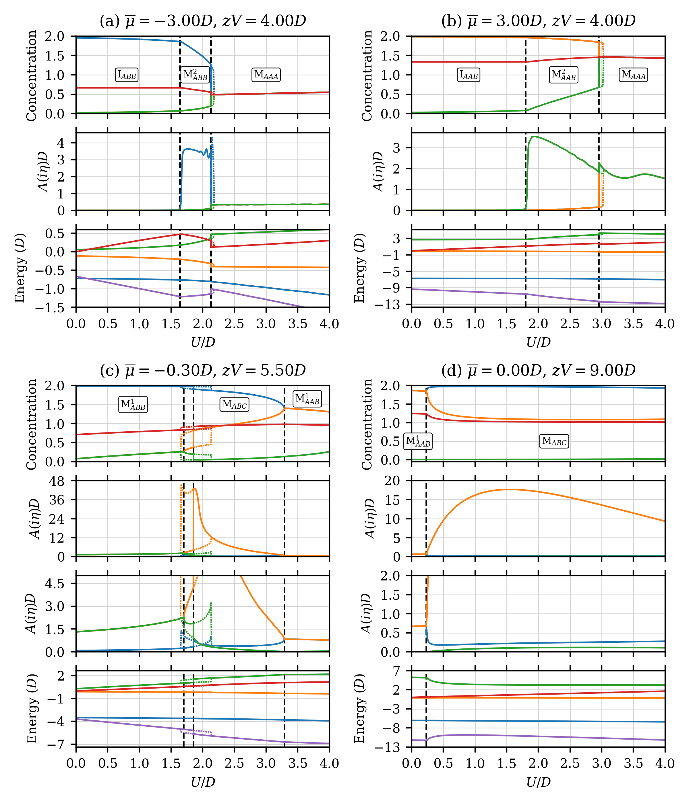
We denote the total concentration . For the analysis of discontinuous phase transitions, the contributions to the grand potential (all per lattice site ) are defined as the thermal averages of the corresponding terms in the Hamiltonian (II): kinetic energy (-term contribution), on-site interaction energy (-term contribution), intersite-interaction energy (-term contribution), potential energy (- and -term contributions together), and chemical energy (-term contribution). At finite temperatures also has a contribution ( is an entropy of the system) which is zero in this research.
One of the advantages of MFA is the ability to plot and analyze a band structure . It is found as eigenvalues of a matrix:
| (15) |
The spectral function is calculated as
| (16) |
where , and are diagonal elements of a matrix
| (17) |
When the spectral function is calculated with such a small , the grid of -points or more is used to make plots of spectral function clear.
The calculations are implemented in the Python language with the use of Matplotlib library for visualization.
III Non-Interacting Limit
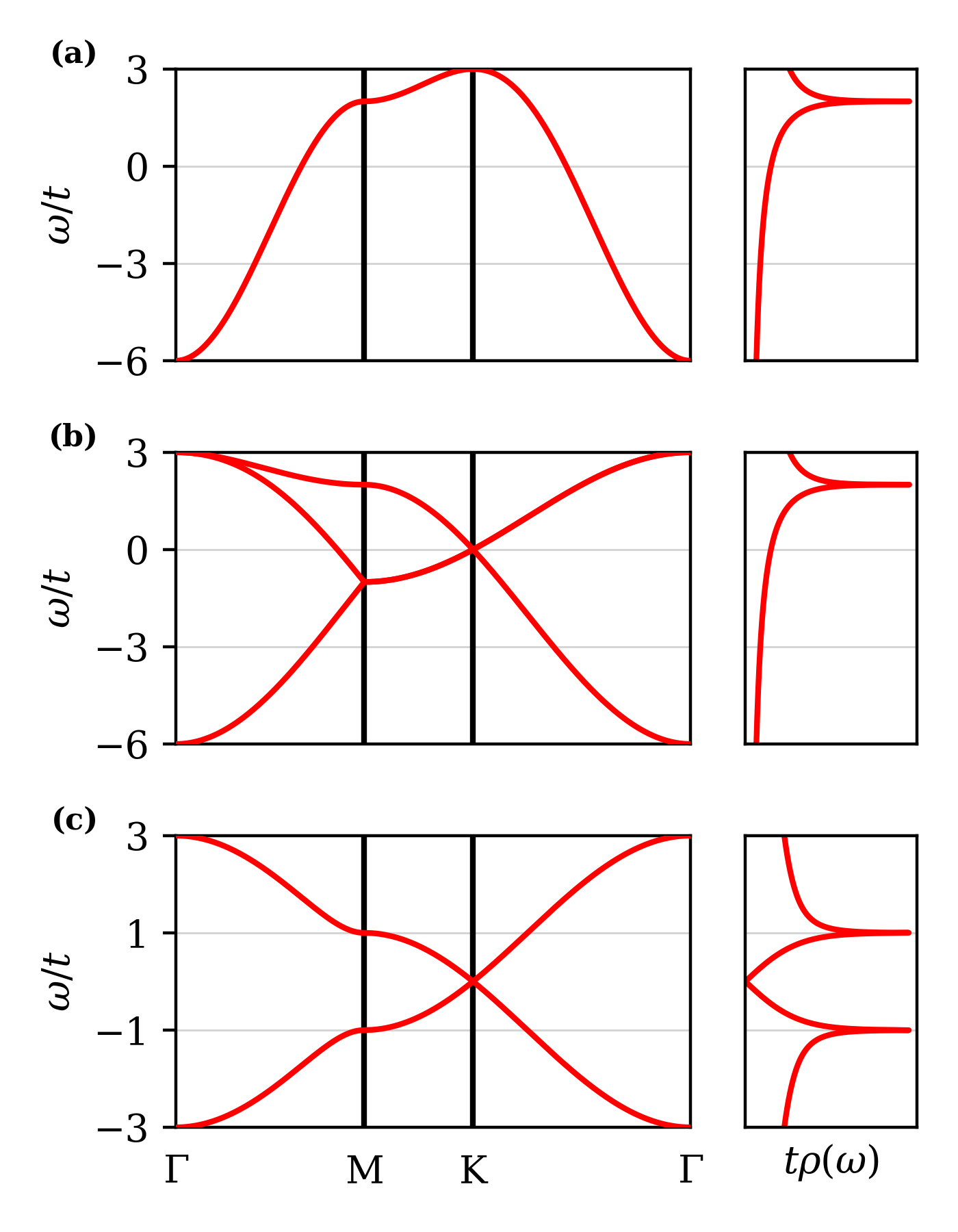
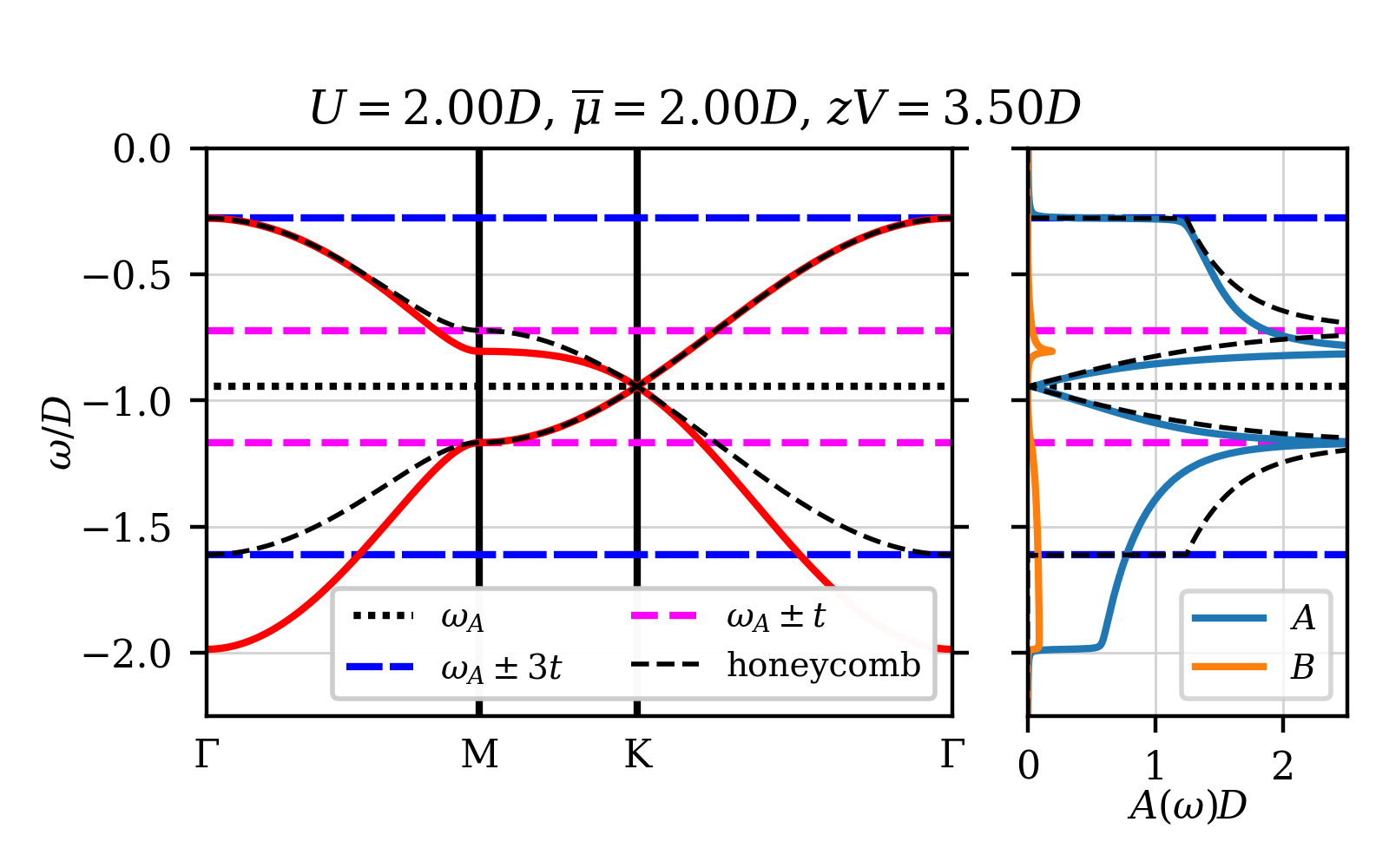
For the reference point and the following analysis, the band structures and the densities of states (DOSs) of non-interacting triangular and honeycomb lattices are presented in Fig. 1. Both the no-sublattice case (Fig. 1a) and the 3-sublattice case with the bands folded in accordance with supercell (Fig. 1b) are shown.
The DOS (per spin) of a triangular lattice is [71]:
| (18) |
where: is the complete elliptic integral of the first kind,
| (19) | |||
It is asymmetric, exists from to , and has a van Hove singularity at . The zero-temperature half-filling would correspond to a Fermi level .
The DOS (per spin) of a honeycomb lattice is [72, 73]:
| (20) |
It is symmetric around the Dirac cone at , exists from to , and has van Hove singularities at (Fig. 1c).
IV Phase Diagram
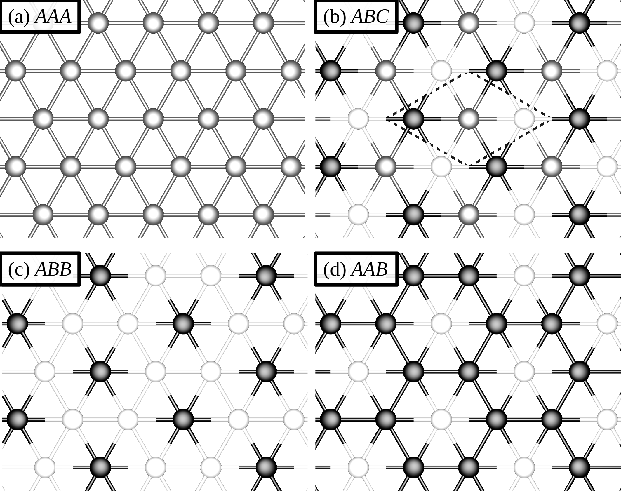
The phase diagram is shown in Fig. 2 while the structures of the found charge orders are schematically presented in Fig. 3. In the model (II), the lattice is fully unoccupied (I000) for and fully occupied (I222) for . The corresponding regions on the phase diagrams are indicated by gray color in Fig. 2.
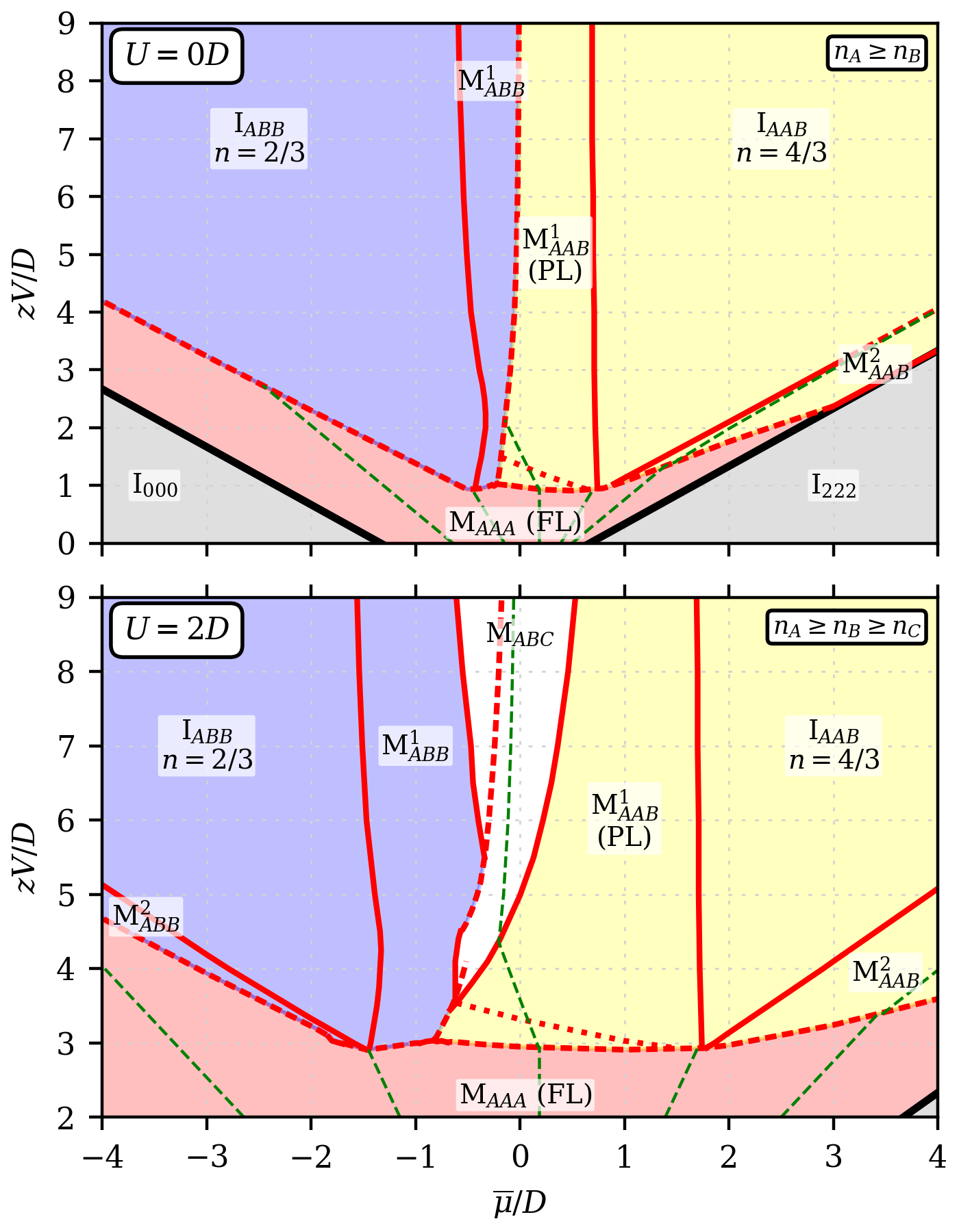
The metallic phase without charge order (CO) is denoted as MAAA or as the Fermi liquid (FL) and marked by the red color. Its band structure and spectral function fully repeat the non-interacting ones (Fig. 1b) except the Fermi level is shifted by:
| (21) |
(cf. Eq. (5) when all are equal). It is possible to have convergence of an algorithm for the non-charge-ordered phase throughout the whole phase diagram. However, the further it goes into the charge-ordered regions of the phase diagram, the easier it can be destabilized toward CO phases by introduction of small deviations in the input , and the larger the difference between its grand potential and the grand potential of the CO phases.
The blue and yellow regions of the phase diagram in Fig. 2 mark the CO phases with the sublattice occupation numbers , ( phases, Fig. 3c) and , ( phases, Fig. 3d), respectively, with . These phases have degeneracy of 3, e.g., the possible sublattice occupation numbers of the yellow region ( region) are , , and .
The yellow region (subsection IV.1) encompasses two CO metallic phases (M and M) and an insulating one (IAAB). The total concentration in the latter is always , while in the atomic-limit case it has the sublattice occupation numbers . The M phase is in fact a so-called pinball liquid (PL) phase, i.e. the electrons cannot hop through one of the sublattices which takes role of pins, while the honeycomb lattice formed by the other two sublattices is metallic. The phase loses its PL properties as it approaches a FL phase (the dotted line).
The blue region in Fig. 2 (subsection IV.2) encompasses two CO metallic phases (M and M) and an insulating one (IABB, ) which in the atomic-limit case has the sublattice occupation numbers .
When , CO metallic phases with the most broken symmetry occur, i.e., all three occupation numbers in the sublattices are different from each other (MABC, white region, Fig. 3b, subsection IV.4). The two phases can be identified in this region: an -like MABC phase and an -like MABC phase. The degeneracy of the phases is .
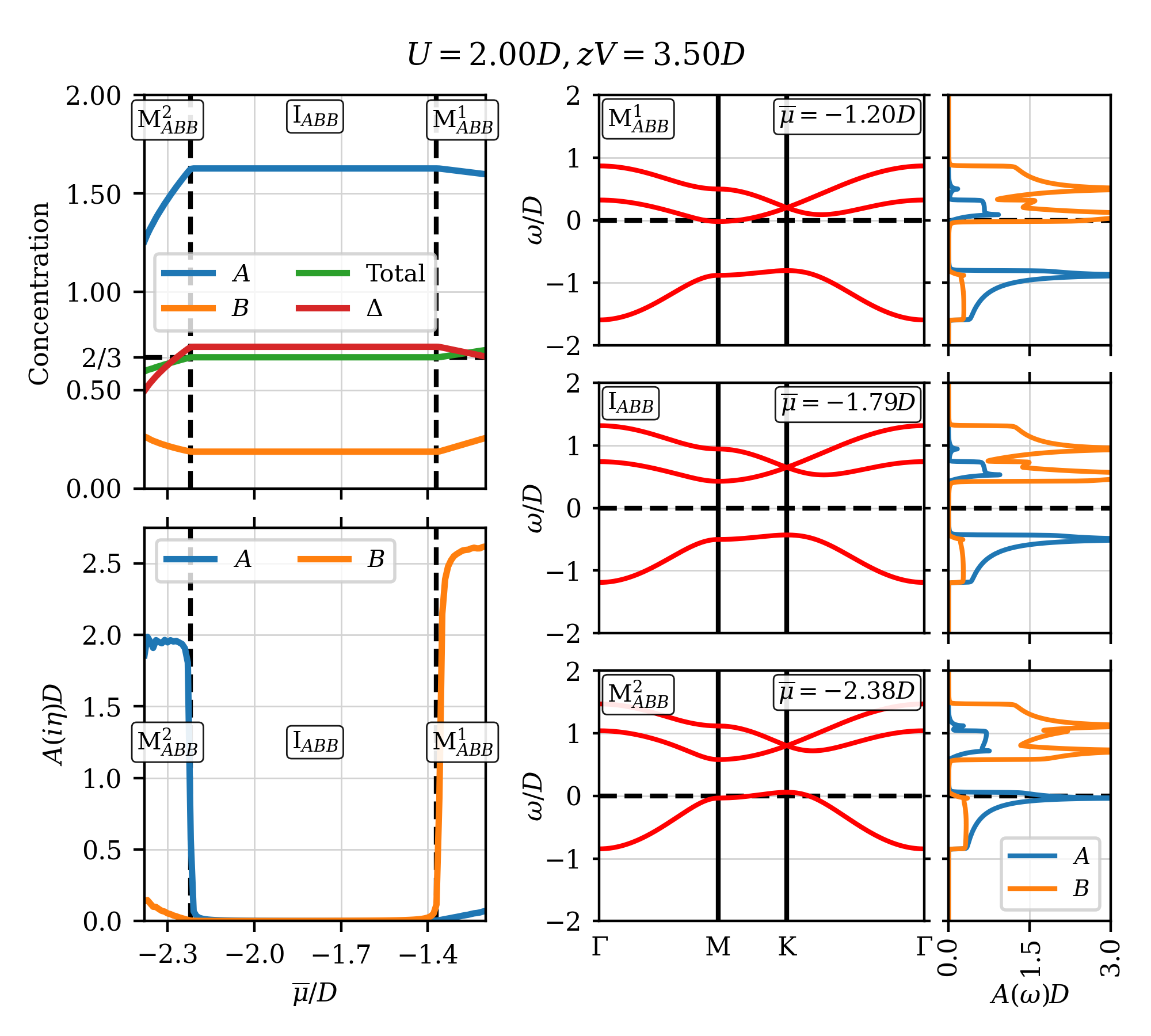
IV.1 AAB Region
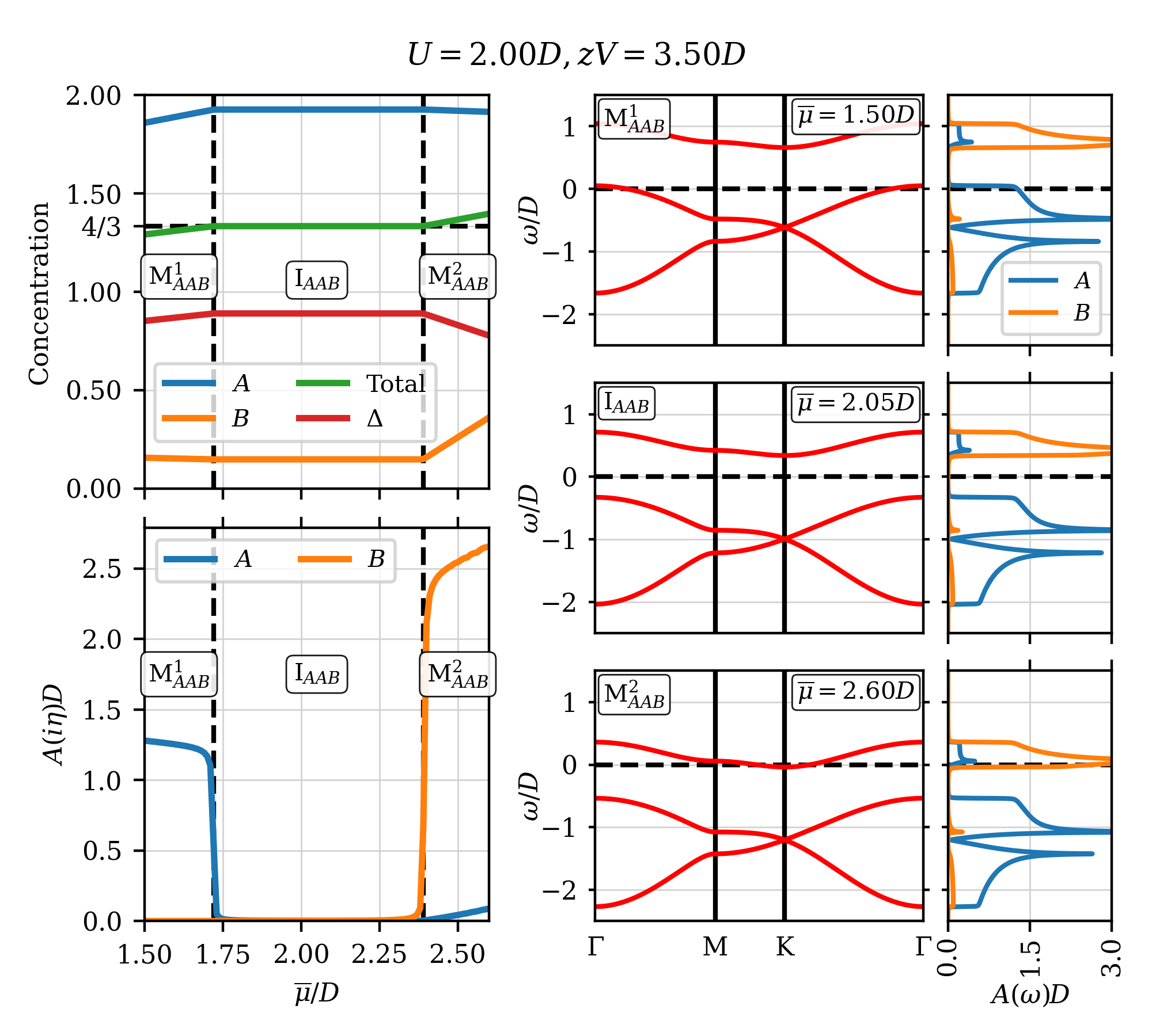
Two continuous phase transitions and the band structures of the phases (yellow-region phases in Fig. 2) are shown in Fig. 4. For the whole band-structure evolution between and for and see the file M1_U2.00_V3.50_AAB.mp4 111See Supplemental Material at [URL will be inserted by publisher] with the results for band structure and evolution of various observables as a function of the model parameters.. Since sublattices in this region are occupied by two different occupation numbers only, the useful order parameter is a polarization
| (22) |
The spectral weight and .
When not in the proximity of the FL or I222 phases (see subsection IV.3), the AAB phases can be described as a separate triangular lattice formed by the sublattice with the occupation (triangular- lattice), a honeycomb lattice represented by the sublattices with the occupation (honeycomb- lattice), and a certain amount of hybridization between them (cf. the non-interacting band structures in Fig. 1a and 1c). The hopping between sites of the triangular- lattice takes place by means of this hybridization with the honeycomb- lattice and hance has a modified amplitude: the opposite sign and a smaller absolute value. As the intersite interaction increases, the hybridization decreases. This turns the triangular-like band into a dispersionless atomic level, while the lower bands become indistinguishable from the non-interacting honeycomb band structure (Fig. 1c) with a shifted Fermi level. For a band-structure evolution with the increase of see the file M2_U2.00_mu2.00_AAB.mp4 [75]. The above is valid for all phases.
Noticeably, a position of a Dirac cone at the K-point of the honeycomb-like bands and a position of an extremum at the K-point of the triangular-like band are always fixed at
| (23) |
respectively, where the distance between them:
| (24) |
The other way to write these expressions is
| (25) |
(in this subsection, and ).
To get more insights on phases, the lower bands (honeycomb-like bands) are shown in Fig. 5 together with and lines where the non-interacting honeycomb band structure has edges and van Hove singularities. It turns out that the upper edge and the lower singularity are always fixed at and , respectively. It justifies the lack of dependency on the interaction of a left boundary of the IAAB phase in Fig. 2. Consequently, the band gap of the IAAB phase:
| (26) |
(asymptotically approaches for a large ).
On the energy scale the hybridization with the triangular- lattice is concentrated around the lower edge and the upper singularity of the honeycomb-like bands. It is clear from the non-zero spectral weight of the triangular- lattice. Locations of these points are not fixed to and , but approach these values in the large- limit where the hybridization disappears (see the file M2_U2.00_mu2.00_AAB.mp4 [75]).
Since there is no spectral weight of the triangular- lattice close to the maximum of the lower bands, the M phase is a pinball liquid. Close to the FL phase, the upper and lower bands start to merge and the phase is not a PL anymore. This transition is continuous and very smooth (see for example Fig. S1d and S1e [75]). To give an approximate boundary of the PL phase, the dotted line in Fig. 2 shows the points where the maximum of the lower bands (located at the -point) and the minimum of the upper band (located at the K-point) have the same energy. From the expressions above it is clear that this line exactly corresponds to .
For or close to , the IAAB-M transition is sharp and gets discontinuous for (see for example Fig. S2a [75]). It can be justified by the proximity of the transition to the fully occupied phase (I222). The total concentration in IAAB and I222 phases is always and , respectively, while the transition between M and I222 phases is continuous (subsection IV.3). As a consequence the sharp change in occupation numbers occurs at the IAAB-M transition. When moving from the CO metallic phase, this discontinuous transition corresponds to the release of the potential energy at the expense of the chemical energy.
It is worth noting, since the M phase exists for any large values of (when is also large), and in the large- limit the hybridization between the honeycomb- and the triangular- lattices disappears, it eventually becomes an insulator: the Fermi level is located in the atomic-like peak formed by the sublattice with the occupation (and both and are not integer!), while the hopping with neighboring sites is restricted. This situation is rather unphysical, and both an inclusion of a next-nearest-neighbor hopping, and an inclusion of the Mott physics can resolve it.
IV.2 ABB Region
The band structures of the phases (blue region in Fig. 2) and phase transitions between them are shown in Fig. 6. For the whole band structure evolution during these transitions see also the file M3_U2.00_V3.50_ABB.mp4 [75]. Here, the spectral weight and .
In the region, honeycomb-like bands of a lattice formed by the sublattices with the occupation (honeycomb- lattice) are located above a triangular-like band of a lattice formed by the sublattice with the occupation (triangular-). It is clear, that the upper bands look less like the honeycomb bands (Fig. 1c) for in comparison to the lower bands for the same . It is justified by the fact that the 1st and the 2nd bands in Fig. 1b can be transformed to the honeycomb bands (Fig. 1c) with less effort than the 2nd and the 3rd bands. When increases, the bands change accordingly to form non-interacting honeycomb-like and triangular-like (eventually, an atomic-like) bands while the hybridization between them disappears: see the file M4_U2.00_mu-1.80_ABB.mp4 [75].
Positions of the K-point extremum of the triangular-like band and the Dirac cone of the honeycomb-like bands are still fixed to the energies defined by Eq. (25) ( and ) or, in terms of the polarization,
| (27) |
Similar to the phases, the upper edge and the lower singularity of the honeycomb-like bands are also fixed to and in contrast to the lower edge and the upper singularity that approach and only in the large- limit when the hybridization disappears. Since, the lower edge is now adjacent to a band gap, the phases are noticeably different from the phases. The right boundary of the IABB phase in Fig. 2 is dependent on . The expression of the lower limit only of the IABB-phase band gap can be written:
| (28) |
When increases, the asymptotically approaches the right-side expression.
Since the hybridization between the honeycomb- and triangular- lattices is concentrated around the minimum of the honeycomb-like bands, exactly where the Fermi level of the M phase is located, the phase is not a PL. In the limit of large the hybridization disappears; hence, in this limit, the M phase would eventually become a PL, but the border of such a transition is vague. Similarly to the M, the M phase in large- limit is an insulator with non-integer occupations which can be viewed as an artifact of a model or its mean-field treating.
In contrast to the region, the M phase does not exist for or close to . The discontinuous transition to the FL phase (subsection IV.3) takes place directly from IABB phase.
IV.3 Symmetry Breaking from a Non-Charge-Ordered Phase
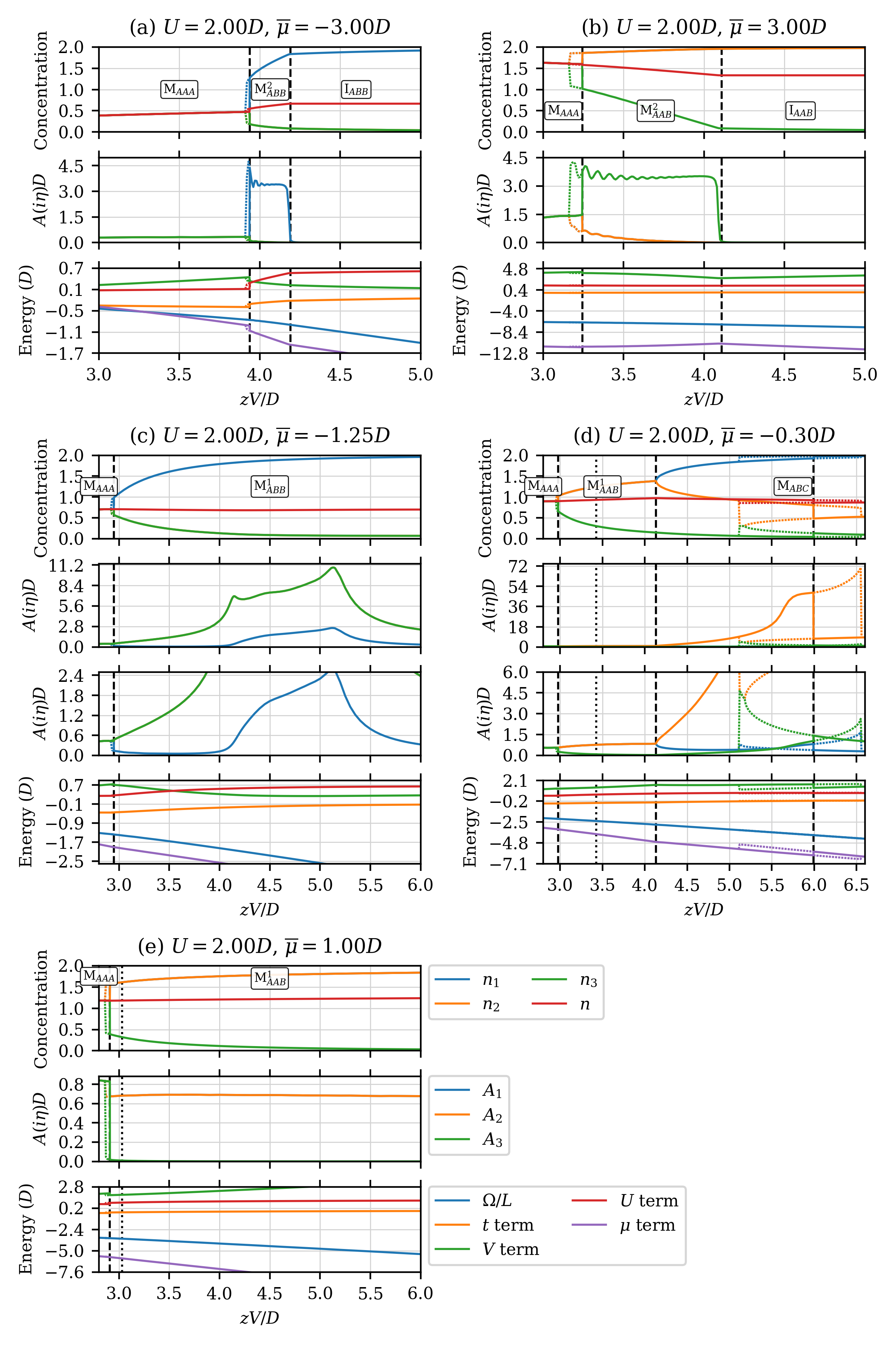
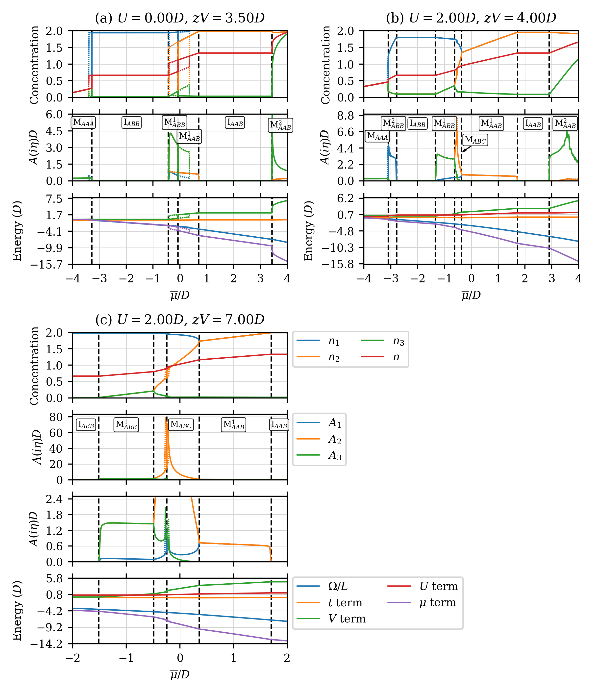
Throughout most of the range of the transitions from the FL phase (MAAA, red region in Fig. 2) to the CO phases (M, M, IABB, M, M, IAAB) are discontinuous (see for example Fig. S1 [75]). Noticeably, these transitions take place for . The discontinuous symmetry breaking corresponds to the release of intersite-interaction energy at the expense of both kinetic and on-site-interaction energy. Additionally, the chemical energy decreases with transitions to the M and IABB phases, and increases with transitions to the M and IABB phases. The CO phases are metastable inside the FL region for a rather small range of parameters: on the axis the span of this range is up to for the most noticeable hysteresis (IABB-MAAA transition for and large hole doping).
The analysis of band structures shows that the CO phases get unstable when the Fermi level approaches certain valleys or saddle points. Moreover, there are ranges of where the symmetry-breaking transitions to the CO metallic phases are continuous (see continuous evolutions in the files M*_SymBreak.mp4 [75]).
IV.3.1 M and IABB Phases
The CO M and IABB phases become unstable when the Fermi level approaches (from above) the maximum of the lower (triangular-like) band located at the K-point (see their phase diagrams in Fig. 6 for the reference).
For the continuous transition to the FL, the maximum of the triangular-like band should merge with the Dirac point of the honeycomb-like bands at the K-point. The Fermi level cannot be above the Dirac point because it destabilizes the M phase towards an phase. However, the Fermi level stays between the maximum of the triangular-like band and the Dirac point close to the triple phase-transition point of the MAAA, M, and M phases. There, the continuous symmetry breaking to the M phase takes place. It is visualized in the file M5_U2.00_mu-0.85_ABB_SymBreak.mp4 [75].
Since the Fermi level appears where all three bands of the FL phase are degenerate at the K-point, the around the continuous transition, i.e.
| (29) |
where is the non-interacting triangular-lattice occupation that corresponds to . Noticeably, around the triple point the which brings us to the expression:
| (30) |
for the triple point.
IV.3.2 M Phase
Similarly, the M phase (but not IAAB) becomes unstable towards the FL phase when the Fermi level approaches (from below) the minimum of the upper (triangular-like) band at the K-point (see its phase diagram in Fig. 4 for the reference). The same as for the M phase, the continuous phase transition (merging the extremum of the triangular-like band and the Dirac point at the K-point) happens around the same triple point of the phase diagram where Eq. (29) is satisfied with the same . The continuous transition is visualized in the file M6_U2.00_mu-0.80_AAB_SymBreak.mp4 [75].
IV.3.3 M Phase
For close to , there is no transition between the FL phase and the M phase. For a larger , the CO phase becomes unstable towards the FL phase in two ways: 1) when the Fermi level approaches (from above) the singularity (saddle point) of the lower (triangular-like) band at the M-point; 2) when the Fermi level approaches (from below) the minimum of the upper (honeycomb-like) bands which in this range of parameters is at the M-point.
The continuous transition between the FL and M phase happens in the small range of when the Fermi level stays in between of the mentioned saddle point and minimum at the M-point. It is visualized in the file M7_U2.00_mu-1.80_ABB_SymBreak.mp4 [75]. Since the Fermi level appears where the two bands of the FL phase are degenerate at the M-point, the around the continuous transition, i.e.
| (31) |
where is the non-interacting triangular-lattice occupation when .
IV.3.4 M and IAAB Phases
The M and IAAB phases become unstable towards the FL phase when the Fermi level approaches (from above) the maximum of the lower (honeycomb-like) bands at the -point.
In contrast to the M, the M phase cannot continuously transform to the FL but has an infinite range of (particularly, ) where it continuously transforms to the fully occupied phase (I222). The continuous transition is visualized in the file M8_U0.00_mu3.10_AAB_SymBreak.mp4 [75].
At this continuous transition the with which corresponds to the top of the non-interacting triangular-lattice bands:
| (32) |
IV.4 AAB-ABB Transition and ABC Region
The transition between the M and M phases (between the yellow and blue regions) is discontinuous (see for example Fig. S2a [75]). When moving from the phase, it happens with the release of chemical energy at the expense of intersite-interaction energy.
For an intermediate region of MABC phases (, , , , white region) opens between the and regions (see for example Fig. S3d [75]). For the most range of parameters the transition between the region and the M phase on one side and the M phase on the other side is continuous. Note that the less-symmetry-broken phases ( and ) can have the self-consistent solution of the Hamiltonian (3) inside the region despite other indicators that the phase transition is continuous.
The region can be characterized by identifying two phases: the -like MABC phase and the -like MABC phase with the discontinuous transition between them. Moreover, there is a range of where the -like MABC phase discontinuously transforms directly into the M phase (see Fig. 2). The same as for the M-M transition, these discontinuous transitions take place with the release of chemical energy at the expense of intersite-interaction energy when moving from the -like side.
There is a range of parameters where the phase can be viewed as both -like and -like MABC phase (in Fig. 2 the region around for ). The visualization of two continuous transitions between the , , and regions for and is presented in the file M9_U2.00_V4.40 _ABB-ABC-AAB.mp4 [75].
The band structure of the MABC phase consists of bands: a lower triangular-like which spectral weight primarily comes from the -sublattice, an upper triangular-like which spectral weight primarily comes from the -sublattice, and an intermediate band which spectral weight primarily comes from the -sublattice. The Fermi level is located inside the intermediate band. All three bands have an extremum at the K-point that is fixed to the energy defined from Eq. (25) (, , and ). In the large- limit the three bands are rather three atomic levels: a fully occupied level, a fully unoccupied level, and a level where the Fermi level is located.
IV.5 Correspondence to the Atomic-Limit Phase Diagram
For a large the atomic-limit solution of the triangular-lattice EHM predicts 7 phases that are denoted according to the three occupation numbers: 000, 100, 200, 210, 220, 221, and 222 [69]. The phase transitions take place at the following lines:
| (33) | |||||
where the ’’ corresponds to the first or second boundary mentioned above, respectively. It is clear from the formulas that the phases 100, 210 and 221 do not exist for .
There is a correspondence between the atomic-limit and mean-field solutions at a large . Besides the obvious correspondence for the fully-unoccupied and fully-occupied phases, the atomic-limit 100 phase can be associated with the mean-field M phase, the 200 phase with the IABB and M phases together, the 210 phase with MABC phase, and correspondingly for the other side of the phase diagram.
Thus, the disappearance of the MABC and M phases for could be predicted from the atomic-limit solution. Despite this correspondence, the mean-field phase M exists even for and large , which makes it an unexpected effect of non-zero itineracy.
To compare the atomic-limit and the mean-field solutions, one can put in Eqs. (IV.5) (despite the fact that in the atomic limit):
The mean-field boundaries of MABC phase at large and indeed slowly approach (Fig. 2). The same is valid for the boundaries of the I000 and I222 phases since the terms and become negligible in comparison to the large . The left boundary of the IABB phase coincide well with the left boundary of the atomic-limit 200 phase even at the small values of , and the same is valid for the 220 and IAAB phases.
It is reasonable to expect that primarily those phases that are associated with non-zero (MABC, M, M) will be modified when taking into account the Mott physics (local correlations). Note also, that in the atomic limit there are also 111 (Mott insulator), 110, and 211 phases for small (particularly, for ).
V Summary
The full zero-temperature phase diagram of the extended Hubbard model on the triangular lattice in the all-encompassing range of chemical potential values and repulsive onsite and nearest-neighbor electron interactions is presented and analyzed. Despite the limitations of the mean-field approximation, restriction to the supercells and the absence of magnetic order, the large variety of features are found. Those are the diverse and numerous phase transitions, including the continuous and discontinuous symmetry breakings; the pinball liquid phase; the strong particle-hole asymmetry manifested in every phase transition with a charge-ordered phase. Both the found phases and the found phase transitions are accompanied by the extensive band-structure analysis that provided clarity and the understanding of the phase diagram. It is worth noting, that the quarter-filling for electrons () and holes () that is common for some organic conductors occurs in the MAAA (FL), M, and M phases, which are not pinball-liquid phases within the MFA.
It is evident that the future investigation beyond the mean-field approximation can benefit from our analysis. Additionally, our research can easily be expanded to include next-nearest-neighbor interactions and finite temperatures. The more work is also required to include magnetic order and to consider the orderings that require larger supercells.
Acknowledgements.
K.J.K. thanks the Polish National Agency for Academic Exchange for funding in the frame of the National Component of the Mieczysław Bekker program (2020 edition) (BPN/BKK/2022/1/00011).References
- Wu et al. [2018] F. Wu, T. Lovorn, E. Tutuc, and A. H. MacDonald, Hubbard model physics in transition metal dichalcogenide moiré bands, Phys. Rev. Lett. 121, 026402 (2018).
- Bistritzer and MacDonald [2011] R. Bistritzer and A. H. MacDonald, Moiré bands in twisted double-layer graphene, PNAS 108, 12233 (2011).
- Chen and Sheng [2023] F. Chen and D. N. Sheng, Singlet, triplet, and pair density wave superconductivity in the doped triangular-lattice moiré system, Phys. Rev. B 108, L201110 (2023).
- Kim et al. [2017] K. Kim, A. DaSilva, S. Huang, B. Fallahazad, S. Larentis, T. Taniguchi, K. Watanabe, B. J. LeRoy, A. H. MacDonald, and E. Tutuc, Tunable moiré bands and strong correlations in small-twist-angle bilayer graphene, PNAS 114, 3364 (2017).
- Cao et al. [2018a] Y. Cao, V. Fatemi, V. Demir, S. Fang, S. L. Tomarken, J. Y. Luo, J. D. Sanchez-Yamagishi, K. Watanabe, T. Taniguchi, K. Kaxiras, R. C. Ashoori, and P. Jarillo-Herrero, Unconventional superconductivity in magic-angle graphene superlattices, Nature 556, 80 (2018a).
- Cao et al. [2018b] Y. Cao, V. Fatemi, V. Demir, S. Fang, S. L. Tomarken, J. Y. Luo, J. D. Sanchez-Yamagishi, K. Watanabe, T. Taniguchi, K. Kaxiras, R. C. Ashoori, and P. Jarillo-Herrero, Correlated insulator behaviour at half-filling in magic-angle graphene superlattices, Nature 556, 43 (2018b).
- Yang et al. [2021] J. Yang, L. Liu, J. Mongkolkiattichai, and P. Schauss, Site-resolved imaging of ultracold fermions in a triangular-lattice quantum gas microscope, PRXQuantum 2, 020344 (2021).
- Struck et al. [2011] J. Struck, C. Ölschläger, R. L. Targat, P. Soltan-Panahi, A. Eckardt, M. Lewenstein, P. Windpassinger, and K. Sengstock, Quantum simulation of frustrated classical magnetism in triangular optical lattices, Science 333, 996 (2011).
- Mathey et al. [2007] L. Mathey, S.-W. Tsai, and A. H. Castro Neto, Exotic superconducting phases of ultracold atom mixtures on triangular lattices, Phys. Rev. B 75, 174516 (2007).
- Yamamoto et al. [2020] D. Yamamoto, T. Fukuhara, and I. Danshita, Frustrated quantum magnetism with Bose gases in triangular optical lattices at negative absolute temperatures, Commun. Phys. 3, 56 (2020).
- Mongkolkiattichai et al. [2023] J. Mongkolkiattichai, L. Liu, D. Garwood, J. Yang, and P. Schauss, Quantum gas microscopy of fermionic triangular-lattice Mott insulators, Phys. Rev. A 108, L061301 (2023).
- Wu et al. [2024] J. Wu, H. Tan, R. Cao, J. Yuan, and Y. Li, Orbital phases of -band ultracold fermions in a frustrated triangular lattice, Phys. Rev. A 110, 043319 (2024).
- Wessel [2007] S. Wessel, Simulations of atomic gases on frustrated optical lattices, Comput. Phys. Commun. 177, 166 (2007).
- Jo et al. [2012] G.-B. Jo, J. Guzman, C. K. Thomas, P. Hosur, A. Vishwanath, and D. M. Stamper-Kurn, Ultracold atoms in a tunable optical kagome lattice, Phys. Rev. Lett. 108, 045305 (2012).
- Kim and Pereg-Barnea [2023] K. W. Kim and T. Pereg-Barnea, Interplay between superconductivity and magnetism in triangular lattices, Phys. Rev. B 108, 195113 (2023).
- Venderley and Kim [2019] J. Venderley and E.-A. Kim, Density matrix renormalization group study of superconductivity in the triangular lattice Hubbard model, Phys. Rev. B 100, 060506 (2019).
- Chen et al. [2013] K. S. Chen, Z. Y. Meng, U. Yu, S. Yang, M. Jarrell, and J. Moreno, Unconventional superconductivity on the triangular lattice Hubbard model, Phys. Rev. B 88, 041103 (2013).
- Jiang [2021] H.-C. Jiang, Superconductivity in the doped quantum spin liquid on the triangular lattice, npj Quantum Materials 7, 71 (2021).
- Horigane et al. [2019] K. Horigane, K. Takeuchi, D. Hyakumura, R. Horie, T. Sato, T. Muranaka, K. Kawashima, H. Ishii, Y. Kubozono, S. Orimo, M. Isobe, and J. Akimitsu, Superconductivity in a new layered triangular-lattice system Li2IrSi2, New J. Phys. 21, 093056 (2019).
- Yamada [2025] A. Yamada, -wave superconductivity in the Hubbard model on the isotropic triangular lattice by the variational cluster approximation, J. Phys. Soc. Jpn. 94, 044705 (2025).
- Watanabe and Ogata [2005] H. Watanabe and M. Ogata, Charge order and superconductivity in two-dimensional triangular lattice at , J. Phys. Soc. Jpn. 74, 2901 (2005).
- Cheng et al. [2024] J. Cheng, J. Bai, B. Ruan, P. Liu, Y. Huang, Q. Dong, Y. Huang, Y. Sun, C. Li, L. Zhang, Q. Liu, W. Zhu, Z. Ren, and G. Chen, Superconductivity in a layered cobalt oxychalcogenide Na2CoSe2O with a triangular lattice, J. Am. Chem. Soc. 146, 5908 (2024).
- Morera et al. [2023] I. Morera, M. Kanász-Nagy, T. Smolenski, L. Ciorciaro, A. m. c. Imamoğlu, and E. Demler, High-temperature kinetic magnetism in triangular lattices, Phys. Rev. Research 5, L022048 (2023).
- Ciorciaro et al. [2023] L. Ciorciaro, T. Smoleński, I. Morera, N. Kiper, S. Hiestand, M. Kroner, Y. Zhang, K. Watanabe, T. Taniguchi, E. Demler, and A. İmamoğlu, High-temperature kinetic magnetism in triangular lattices, Nature 623, 509 (2023).
- Khatua et al. [2022] J. Khatua, M. Pregelj, A. Elghandour, Z. Jagličic, R. Klingeler, A. Zorko, and P. Khuntia, Magnetic properties of the triangular-lattice antiferromagnets , Phys. Rev. B 106, 104408 (2022).
- Sala et al. [2023] G. Sala, M. B. Stone, S.-H. Do, K. M. Taddei, Q. Zhang, G. B. Halász, M. D. Lumsden, A. F. May, and A. D. Christianson, Structure and magnetism of the triangular lattice material YbBO3, J. Phys.: Condens. Matter 35, 395804 (2023).
- Ferreira et al. [2020] T. Ferreira, J. Xing, L. D. Sanjeewa, and A. S. Sefat, Frustrated magnetism in triangular lattice TlYbS2 crystals grown via molten flux, Front. Chem. 8, 127 (2020).
- Ogunbunmi and Strydom [2022] M. O. Ogunbunmi and A. M. Strydom, Physical and magnetic properties of frustrated triangular-lattice antiferromagnets R3Cu (R = Ce, Pr), J. Alloys Compd. 895, 162545 (2022).
- Xing et al. [2020] J. Xing, L. D. Sanjeewa, J. Kim, G. R. Stewart, M.-H. Du, F. A. Reboredo, R. Custelcean, and A. S. Sefat, Crystal synthesis and frustrated magnetism in triangular lattice CsRESe2 (RE = La–Lu): Quantum spin liquid candidates CsCeSe2 and CsYbSe2, ACS Materials Lett. 2, 71 (2020).
- Isono et al. [2020] T. Isono, Y. Machida, and W. Fujita, Low-temperature magnetism in a triangular-lattice antiferromagnet, Cu3(OH)4(HCO2)2, studied by calorimetry, J. Phys. Soc. Jpn. 89, 073707 (2020).
- Yoshioka et al. [2009] T. Yoshioka, A. Koga, and N. Kawakami, Quantum phase transitions in the Hubbard model on a triangular lattice, Phys. Rev. Lett. 103, 036401 (2009).
- Shirakawa et al. [2017] T. Shirakawa, T. Tohyama, J. Kokalj, S. Sota, and S. Yunoki, Ground-state phase diagram of the triangular lattice Hubbard model by the density-matrix renormalization group method, Phys. Rev. B 96, 205130 (2017).
- Jiang and Jiang [2020] Y.-F. Jiang and H.-C. Jiang, Topological superconductivity in the doped chiral spin liquid on the triangular lattice, Phys. Rev. Lett. 125, 157002 (2020).
- Szasz et al. [2020] A. Szasz, J. Motruk, M. P. Zaletel, and J. E. Moore, Chiral spin liquid phase of the triangular lattice Hubbard model: A density matrix renormalization group study, Phys. Rev. X 10, 021042 (2020).
- Noda and Imada [2002] Y. Noda and M. Imada, Quantum phase transitions to charge-ordered and wigner-crystal states under the interplay of lattice commensurability and long-range coulomb interactions, Phys. Rev. Lett. 89, 176803 (2002).
- Hiraki and Kanoda [1998] K. Hiraki and K. Kanoda, Wigner crystal type of charge ordering in an organic conductor with a quarter-filled band: , Phys. Rev. Lett. 80, 4737 (1998).
- Tan et al. [2023] Y. Tan, P. K. H. Tsang, V. Dobrosavljević, and L. Rademaker, Doping a Wigner-Mott insulator: Exotic charge orders in transition metal dichalcogenide moiré heterobilayers, Phys. Rev. Research 5, 043190 (2023).
- Matty and Kim [2022] M. Matty and E.-A. Kim, Melting of generalized wigner crystals in transition metal dichalcogenide heterobilayer Moiré systems, Nat. Commun. 13, 7098 (2022).
- Kuramoto [1978] Y. Kuramoto, Wigner crystal, electron chain, and charge density wave in strong magnetic fields, J. Phys. Soc. Jpn. 44, 1572 (1978).
- Zarenia et al. [2017] M. Zarenia, D. Neilson, and F. M. Peeters, Inhomogeneous phases in coupled electron-hole bilayer graphene sheets: Charge density waves and coupled Wigner crystals, Sci. Rep. 7, 11510 (2017).
- Pankov and Dobrosavljević [2008] S. Pankov and V. Dobrosavljević, Self-doping instability of the wigner-mott insulator, Phys. Rev. B 77, 085104 (2008).
- Amaricci et al. [2010] A. Amaricci, A. Camjayi, K. Haule, G. Kotliar, D. Tanasković, and V. Dobrosavljević, Extended hubbard model: Charge ordering and wigner-mott transition, Phys. Rev. B 82, 155102 (2010).
- Mikolajick et al. [2021] T. Mikolajick, S. Slesazeck, H. Mulaosmanovic, M. H. Park, S. Fichtner, P. D. Lomenzo, M. Hoffmann, and U. Schroeder, Next generation ferroelectric materials for semiconductor process integration and their applications, J. Appl. Phys. 129, 100901 (2021).
- Hotta and Furukawa [2006] C. Hotta and N. Furukawa, Strong coupling theory of the spinless charges on triangular lattices: Possible formation of a gapless charge-ordered liquid, Phys. Rev. B 74, 193107 (2006).
- Hotta and Furukawa [2007] C. Hotta and N. Furukawa, Filling dependence of a new type of charge ordered liquid on a triangular lattice system, J. Phys.: Condens. Matter 19, 145242 (2007).
- Merino et al. [2013] J. Merino, A. Ralko, and S. Fratini, Emergent heavy fermion behavior at the Wigner-Mott transition, Phys. Rev. Lett. 111, 126403 (2013).
- Ralko et al. [2015] A. Ralko, J. Merino, and S. Fratini, Pinball liquid phase from hund’s coupling in frustrated transition-metal oxides, Phys. Rev. B 91, 165139 (2015).
- Trousselet et al. [2012] F. Trousselet, A. Ralko, and A. M. Oleś, Valence bond crystal and possible orbital pinball liquid in a orbital model, Phys. Rev. B 86, 014432 (2012).
- Miyazaki et al. [2009] M. Miyazaki, C. Hotta, S. Miyahara, K. Matsuda, and N. Furukawa, Variational monte carlo study of a spinless fermion t–v model on a triangular lattice: Formation of a pinball liquid, Journal of the Physical Society of Japan 78, 014707 (2009).
- Rakic et al. [2024] M. Rakic, A. F. Ho, and D. K. K. Lee, Elastic properties and thermodynamic anomalies of supersolids, Phys. Rev. Res. 6, 043040 (2024).
- Micnas et al. [1990] R. Micnas, J. Ranninger, and S. Robaszkiewicz, Superconductivity in narrow-band systems with local nonretarded attractive interactions, Rev. Mod. Phys. 62, 113 (1990).
- Rościszewski and Oleś [2003] K. Rościszewski and A. M. Oleś, Charge order in the extended hubbard model, J. Phys.: Condens. Matter 15, 8363 (2003).
- Hirsch [1984] J. E. Hirsch, Charge-density-wave to spin-density-wave transition in the extended hubbard model, Phys. Rev. Lett. 53, 2327 (1984).
- Lin and Hirsch [1986] H. Q. Lin and J. E. Hirsch, Condensation transition in the one-dimensional extended hubbard model, Phys. Rev. B 33, 8155 (1986).
- Clay et al. [1999] R. T. Clay, A. W. Sandvik, and D. K. Campbell, Possible exotic phases in the one-dimensional extended hubbard model, Phys. Rev. B 59, 4665 (1999).
- Penc and Mila [1994] K. Penc and F. Mila, Phase diagram of the one-dimensional extended hubbard model with attractive and/or repulsive interactions at quarter filling, Phys. Rev. B 49, 9670 (1994).
- Calandra et al. [2002] M. Calandra, J. Merino, and R. H. McKenzie, Metal-insulator transition and charge ordering in the extended hubbard model at one-quarter filling, Phys. Rev. B 66, 195102 (2002).
- Davoudi and Tremblay [2006] B. Davoudi and A.-M. S. Tremblay, Nearest-neighbor repulsion and competing charge and spin order in the extended hubbard model, Phys. Rev. B 74, 035113 (2006).
- Litak and Wysokiński [2017] G. Litak and K. I. Wysokiński, Evolution of the charge density wave order on the two-dimensional hexagonal lattice, J. Magn. Magn. Mater. 440, 104 (2017).
- Kaneko and Ogata [2006] M. Kaneko and M. Ogata, Mean-field study of charge order with long periodicity in -(BEDT-TTF) 2X, J. Phys. Soc. Jpn. 75, 014710 (2006).
- Ung et al. [2023] S. F. Ung, J. Lee, and D. R. Reichman, Competing generalized Wigner crystal states in moiré heterostructures, Phys. Rev. B 108, 245113 (2023).
- Pan et al. [2020] H. Pan, F. Wu, and S. Das Sarma, Quantum phase diagram of a Moiré-hubbard model, Phys. Rev. B 102, 201104 (2020).
- Georges et al. [1996] A. Georges, G. Kotliar, W. Krauth, and M. J. Rozenberg, Dynamical mean-field theory of strongly correlated fermion systems and the limit of infinite dimensions, Rev. Mod. Phys. 68, 13 (1996).
- Pietig et al. [1999] R. Pietig, R. Bulla, and S. Blawid, Reentrant charge order transition in the extended hubbard model, Phys. Rev. Lett. 82, 4046 (1999).
- Tong et al. [2004] N.-H. Tong, S.-Q. Shen, and R. Bulla, Charge ordering and phase separation in the infinite dimensional extended hubbard model, Phys. Rev. B 70, 085118 (2004).
- Kapcia and Robaszkiewicz [2011] K. Kapcia and S. Robaszkiewicz, The effects of the next-nearest-neighbour density–density interaction in the atomic limit of the extended Hubbard model, J. Phys.: Condens. Matter 23, 105601 (2011).
- Kapcia and Robaszkiewicz [2016] K. Kapcia and S. Robaszkiewicz, On the phase diagram of the extended Hubbard model with intersite density–density interactions in the atomic limit, Physica A 461, 487 (2016).
- Kapcia et al. [2017] K. Kapcia, S. Robaszkiewicz, M. Capone, and A. Amaricci, Doping-driven metal-insulator transitions and charge orderings in the extended Hubbard model, Phys. Rev. B 95, 125112 (2017).
- Kapcia [2021] K. J. Kapcia, Charge-order on the triangular lattice: A mean-field study for the lattice fermionic gas, Nanomaterials 11, 1181 (2021).
- Kapcia [2022] K. J. Kapcia, Charge-order on the triangular lattice: Effects of next-nearest-neighbor attraction in finite temperatures, . Magn. Magn. Mater. 541, 168441 (2022).
- Hanisch et al. [1997] T. Hanisch, G. S. Uhrig, and E. Müller-Hartmann, Lattice dependence of saturated ferromagnetism in the Hubbard model, Phys. Rev. B 56, 13960 (1997).
- Kogan and Gumbs [2021] E. Kogan and G. Gumbs, Green’s functions and DOS for some 2D lattices, Graphene 10, 1 (2021).
- Cichy et al. [2022] A. Cichy, K. J. Kapcia, and A. Ptok, Connection between the semiconductor-superconductor transition and the spin-polarized superconducting phase in the honeycomb lattice, Phys. Rev. B 105, 214510 (2022).
- Momma and Izumi [2011] K. Momma and F. Izumi, Vesta3 for three-dimensional visualization of crystal, volumetric and morphology data, J. Appl. Crystallogr. 44, 1272 (2011).
- Note [1] See Supplemental Material at [URL will be inserted by publisher] with the results for band structure and evolution of various observables as a function of the model parameters.
Supplemental Material
Particle-Hole Asymmetry and Pinball Liquid in a Triangular-Lattice Extended Hubbard Model within Mean-Field Approximation
Aleksey Alekseev,1 Agnieszka Cichy,1,2 Konrad Jerzy Kapcia,1
1Institute of Spintronics and Quantum Information, Faculty of Physics and Astronomy, Adam Mickiewicz University in Poznań,
Uniwersytetu Poznańskiego 2, PL-61614 Poznań, Poland
2Institut für Physik, Johannes Gutenberg-Universität Mainz, Staudingerweg 9, D-55099 Mainz, Germany
(Dated: May 5, 2025)
In this Supplemental Material we present additional results which clarify the findings included in the main text and extend the discussion, in particular, concerning:
S1 The Dependencies of Order parameters and Grand-potential Contributions
Figures S1, S2, and S3 show the order parameters and the contributions in the grand potential as a function of , , and , respectively. The metastability of the phases (hysteresis) is also shown with dotted lines. In some cases the spectral weight at the Fermi level () is shown on two different scales due to its proximity to a spectral-weight singularity in the and phases. In particular, the figures contain the results for the following model parameters:
In addition, we present nine multimedia movies that show the evolution of the band structure and density of states:
-
1.
M1_U2.00_V3.50_AAB.mp4
— evolution between and for and (transitions M-IAAB and IAAB-M) -
2.
M2_U2.00_mu2.00_AAB.mp4
— evolution between and for and -
3.
M3_U2.00_V3.50_ABB.mp4
— evolution between and for and (transitions M-IABB and IABB-M) -
4.
M4_U2.00_mu-1.80_ABB.mp4
— evolution between and for and -
5.
M5_U2.00_mu-0.85_ABB_SymBreak.mp4
— evolution between and for and (transition MAAA-M) -
6.
M6_U2.00_mu-0.80_AAB_SymBreak.mp4
— evolution between and for and (transition MAAA-M) -
7.
M7_U2.00_mu-1.80_ABB_SymBreak.mp4
— evolution between and for and (transitions MAAA-M and M-IABB) -
8.
M8_U0.00_mu3.10_AAB_SymBreak.mp4
— evolution between and for and (transition I222-M) -
9.
M9_U2.00_V4.40_ABB-ABC-AAB.mp4
— evolution between and for and (transitions M-MABC and MABC-M)
S2 Transitions Found in the System
The list of 24 phase transitions:
-
1.
-metal-insulator transitions (blue region):
-
1.1
M to IABB (continuous);
-
1.2
M to IABB (continuous);
-
1.1
-
2.
-metal-insulator transitions (yellow region):
-
2.1
M to IAAB (continuous);
-
2.2
M to IAAB (continuous);
-
2.3
M to IAAB (discontinuous), for large but small ;
-
2.1
-
3.
FL to transitions (red to blue):
-
3.1
MAAA to M (discontinuous);
-
3.2
MAAA to M (continuous), a small region in the very proximity of M-M transition;
-
3.3
MAAA to M (discontinuous), not for small ;
-
3.4
MAAA to M (continuous), a small region, not for small ;
-
3.5
MAAA to IABB (discontinuous);
-
3.1
-
4.
FL to transitions (red to yellow):
-
4.1
MAAA to M (discontinuous);
-
4.2
MAAA to M (continuous), a small region in the very proximity of M-M transition;
-
4.3
MAAA to M (discontinuous);
-
4.4
MAAA to IAAB (discontinuous);
-
4.1
-
5.
M-M transition (blue to yellow) (discontinuous);
-
6.
region (blue-white-yellow):
-
6.1
MABC to M (continuous);
-
6.2
MABC to M (continuous);
-
6.3
inside the MABC the discontinuous transition from -like MABC phase to -like MABC phase. As shown on phase diagram, there is a region where this transition disappears (the line is terminated)
-
6.4
directly from -like MABC phase to M phase (discontinuous);
-
6.1
-
7.
The M phase is not a PL as it gets closer to M-MAAA-M triple point. The approximate border between M-PL and M-non-PL is the dotted line;
-
8.
In the limit of large , the M phase becomes a PL because the hybridization between triangular and honeycomb lattices disappears, but the border of this phase is hard to define;
-
9.
Additionally, there is one transition from FL to the fully unoccupied phase, and two transitions to the fully occupied phase: from FL and directly from M phase.