*latexText page 1 contains only floats
Neural semi-Lagrangian method for high-dimensional advection-diffusion problems
Abstract
This work is devoted to the numerical approximation of high-dimensional advection-diffusion equations. It is well-known that classical methods, such as the finite volume method, suffer from the curse of dimensionality, and that their time step is constrained by a stability condition. The semi-Lagrangian method is known to overcome the stability issue, while recent time-discrete neural network-based approaches overcome the curse of dimensionality. In this work, we propose a novel neural semi-Lagrangian method that combines these last two approaches. It relies on projecting the initial condition onto a finite-dimensional neural space, and then solving an optimization problem, involving the backwards characteristic equation, at each time step. It is particularly well-suited for implementation on GPUs, as it is fully parallelizable and does not require a mesh. We provide rough error estimates, and present several high-dimensional numerical experiments to assess the performance of our approach, and compare it to other neural methods.
1 Introduction
In this work, we are interested in solving high-dimensional advection-diffusion equations. The large dimensionality may be inherent, for instance in kinetic equations (kinetic transport, Vlasov, or Fokker-Planck equations), where the unknown typically depends on time, space and velocity. It can also be parametric (examples include equations with parametric source terms, differential operators, or boundary conditions). Traditional numerical methods, such as finite difference, finite volume, or finite element methods, applied to such high-dimensional problems, require numerous degrees of freedom to achieve a given level of accuracy. Indeed, the number of degrees of freedom grows as , where is the number of degrees of freedom in each dimension and is the number of dimensions. Thus, grows exponentially with , leading to a curse of dimensionality. This exponential growth is a major obstacle to the numerical solution of high-dimensional kinetic equations, since it leads to a large computational cost and large memory requirements.
With the tremendous progress made in machine learning since the early 2010s, the use of neural network-based methods such as Physics Informed Neural Networks (PINNs) [51, 37, 18] or the Deep Ritz method [21] has significantly grown. In such methods, the solution itself is expressed as a neural network, whose parameters are adjusted such that the equation is satisfied in strong or weak form. These methods have produced good results for elliptic Partial Differential Equations (PDEs) in low or high physical or parametric dimensions, see e.g. [58, 3, 32]. There are also a few applications to high-dimensional transport, although these remain more limited [45, 65, 33]. Indeed, as will be detailed later, PINNs is a spacetime method, which treat space and time in the same way and specific techniques have to be considered to incorporate causality in the training to properly capture the solution, see [61]. For time-dependent equations, another strategy is to use neural networks approximations as functions of space only, and make the neural network parameters evolve in time. This led to the development of the discrete PINNs [57, 5] or Neural Galerkin [40, 29, 9, 34] methods. These methods can be seen as extensions of the classical implicit and explicit Galerkin methods, where the finite-dimensional approximation linear subspace has been replaced with a submanifold of neural networks.
When considering advection equations and even advection-diffusion equations in high dimension, however, semi-Lagrangian approaches [56, 55, 28, 63, 15, 64] are known to be more efficient than standard Galerkin method. At each time step, by using the backward integration of the characteristic curves, the solution is transported exactly before being projected onto the spatial approximation space. Thus, although it is explicit, the scheme has no time step constraints, which reduces the computational cost. Neural networks have been used to improve the accuracy of semi-Lagrangian methods [38, 13, 12]. However, as explained above, numerical simulations for high-dimensional problems are still hard to perform due to the large number of required degrees of freedom. To overcome this difficulty, tensor and low-rank approaches have been developed recently for kinetic dynamics, see e.g. [35, 22, 66] or the review [23].
In order to tackle transport dynamics in large dimension, we propose in this work to combine the semi-Lagrangian approach with neural approximations. The classical projection onto a linear subspace at each time step of the transported solution is then replaced with an optimization process to fit the parameters. This approach constitutes a semi-Lagrangian variant of the discrete PINN method. In the following, we will apply this method to the following parametric advection-diffusion problem, describing the dynamics of an unknown , depending on time variable , space variable and a set of physical parameters. The PDE writes:
| (1.1) |
where is the advection field and is the constant diffusion coefficient. The parameters may appear in the boundary or initial conditions, or in the advection field. We will formally write the PDE without initial and boundary conditions as
| (1.2) |
where the operator is linear in and contains no time derivatives of , or as
| (1.3) |
where the operator is linear in and involves both time and space derivatives. For the remainder of the paper, we assume that the velocity field is known and is not determined by another equation.
The paper is organized as follows. In Section 2, we introduce the classical numerical approaches for this problem and their neural extensions. This discussion illustrates that our approach naturally follows from previous work. Then, in Section 3, we derive the proposed method for pure advection equations, and extend it to advection-diffusion equations. Algorithms and error estimates are provided. Finally, in Section 4, we provide several validation experiments, for both pure advection and advection-diffusion equations, in high-dimensional settings. Section 5 concludes the paper.
2 Classical and neural numerical methods
The goal of this section is to highlight the key differences between classical and neural methods, and to cast the latter into a formalism well-known in the case of classical methods. To that end, Section 2.1 is devoted to classical methods, while Section 2.2 tackles neural methods. We introduce an infinite-dimensional Hilbert space such that , where is the solution to the partial differential equation (1.1). In both Section 2.1 and Section 2.2, this function space will be approximated by a finite-dimensional subspace, denoted by and for classical and neural methods, respectively. The main difference between these two finite-dimensional subspaces is that, while is a linear subspace spanned by some given basis functions, is no longer linear. It may become a submanifold of , depending on the nonlinearity. As such, projecting an element of onto amounts to solving linear systems (or quadratic optimization problems), while projecting it onto requires solving nonlinear, usually non-convex, optimization problems.
First, Section 2.1 introduces three families of classical methods for advection-diffusion equations. These approaches all use Galerkin projections onto a finite-dimensional subspace to represent the PDE solution. Namely, we present the spacetime Galerkin method in Section 2.1.1, the Galerkin method in Section 2.1.2, and the semi-Lagrangian Galerkin method in Section 2.1.3. Second, we discuss neural numerical methods in Section 2.2. We briefly recall that PINNs (Section 2.2.1) and their time-discrete counterparts (Section 2.2.2) can be seen as extensions of classical approaches, where the projection onto a finite-dimensional subspace (finite element space, spectral basis, etc.) is replaced by a projection onto the manifold defined by neural networks with given architectures.
For simplicity, in this section, we drop the dependence on the parameter in the solution . We also do not discuss boundary and initial conditions. Moreover, throughout this section, denotes the approximate solution of the PDE, obtained by the numerical method under consideration in each specific paragraph.
2.1 Classical methods
As mentioned above, classical approaches to solve time-dependent PDEs approximate the solution by projecting the equation onto a finite-dimensional linear subspace of the Hilbert space . To properly introduce this linear subspace, let , and define basis functions . Examples of basis functions include piecewise polynomial functions for finite element methods or Fourier basis functions for spectral methods. The approximate solution then belongs to the -dimensional linear subspace , defined using the basis functions by
where denotes the inner product in and . The goal is to find the degrees of freedom (dofs) that define . These dofs will depend on the choice of basis functions and on the equation to solve. Since we are considering linear equations and projections onto the linear subspace , the dofs will end up being determined by solving linear systems.
2.1.1 Spacetime Galerkin method
In the spacetime Galerkin method (see e.g. [50]), the basis functions depend on both space and time. The solution is approximated, for all and , by
| (2.1) |
Now, to derive the equation for the dofs , we plug the spacetime Galerkin approximation (2.1) into the PDE (1.3), and integrate over the spacetime slab against some test function. We obtain, for all ,
Using (2.1), we obtain
and so
This leads to the linear system , where the components of the mass matrix are defined by
The solution of this linear system then gives the dofs .
2.1.2 Galerkin method
Now, assume that the basis functions only depend on space, and that the dofs depend on time. The idea is to approximate the solution at each discrete time using these space-dependent basis functions. This is equivalent to stating that the linear combination of the basis functions used to represent the solution depends on time. Thus, the approximate solution at time and position is given by
| (2.2) |
We now plug the Galerkin approximation (2.2) into the PDE (1.2), and we integrate over against some test function. We obtain, for all ,
Using the expression (2.2) yields
which we recast as
We finally obtain a linear ODE on the dofs, which reads
where the components of the matrices and are defined by
This linear ODE is then solved using a time-stepping method. We also refer to [50] for more details.
2.1.3 Semi-Lagrangian Galerkin Method
The Galerkin semi-Lagrangian method is a subset of the Galerkin method, specifically designed for advection and advection-diffusion equations. The idea is to avoid the time step restriction by using a Lagrangian approach [20, 48]. We still write the approximate solution under the form (2.2).
We introduce the method in the specific case of a pure transport equation, i.e., when in (1.1). The exact solution satisfies, for all , and ,
| (2.3) |
where is the (backwards) characteristic curve implicitly defined by the ODE
| (2.4) |
Using this, we can formulate the Semi-Lagrangian Galerkin method. To do this, we approximate by in (2.3), and integrate over against a test function. We thus impose that our approximate solution must satisfy, for all and ,
Plugging the Galerkin approximation (2.2) into the above equation, we obtain
Thus, from some known degrees of freedom at some time , we can compute the degrees of freedom at time by solving the above linear system. This is achieved without a stability condition linking to , contrary to the previous methods.
In practice, we define a time discretization , with , and we obtain by projecting the initial condition onto the Galerkin basis. Then, at each time step, is computed by solving
The above linear system is rewritten as
where the elements of mass matrix are defined by
Thanks to this formulation, this method does not have a time step restriction on . As an example, if is a constant vector field, solving (2.4) is immediate, and we get . In this case, the components of the mass matrix simply read
Moreover, if a discontinuous Galerkin basis is used, the mass matrix becomes diagonal, rendering the method particularly efficient [16, 53].
The method can also be extended to advection-diffusion equations, see e.g. [6]. We do not detail this extension here, but the same principle applies. Namely, the feet of the characteristic curves still have to be computed as in the pure advection case. Then, in the presence of diffusion, these feet have to be split into several diffusion directions.
2.2 Neural methods
We now recall some recent neural numerical methods. In such methods, as mentioned above, the approximate function space is no longer a linear subspace spanned by basis functions, but a nonlinear subspace (usually, a submanifold) defined by parameterized nonlinear functions (usually, neural networks). However, it remains finite-dimensional, and the degrees of freedom are the weights of the nonlinear functions. To be clear, let
| (2.5) | ||||
be a parameterized nonlinear function, typically a neural network. Its input will either be , to define spacetime neural methods, or , to define time-discrete neural methods. In the first case, ; in the second one, . Approximating the PDE solution by such nonlinear functions leads to a nonlinear approximation space. Thus, one now expects to solve nonlinear optimization problems, rather than linear systems, to find the dofs . Remark that nonlinear optimization problems have to be solved even when approximating linear equations.
Note that the dofs of the nonlinear function remain denoted by . For instance, if is a neural network, then the dofs are nothing but the weights and biases of the network. Similarly to Section 2.1, the dependence of the dofs in space and time alters the nature of the neural method. Namely, dofs that depend on neither space nor time lead to PINNs, discussed in Section 2.2.1, while time-dependent dofs lead to discrete PINNs and the neural Galerkin method, discussed in Section 2.2.2.
2.2.1 Physics-Informed Neural Networks (PINNs)
To introduce PINNs [51, 37, 18], let us define the nonlinear subspace
The function depends on both space and time. To highlight this dependence, and to distinguish the parameters from the space and time variables, we introduce the notation
Then, a function is written as
Note that depends on both space and time, similarly to the spacetime Galerkin method.
Finding the dofs then consists in directly minimizing, over the spacetime slab, the residual of the PDE (1.3) applied to the approximate solution . This leads to the nonlinear optimization problem
| (2.6) |
It is usually solved using stochastic gradient methods, discretizing the integral with the Monte-Carlo algorithm.
2.2.2 Discrete PINNs and the Neural Galerkin method
Discrete PINNs and the Neural Galerkin method take up the ideas behind the Galerkin method, but applied to the context of nonlinear function spaces. Namely, we replace the approximation space with
The function still depends on space, time, and dofs, but its time dependence is no longer explicit; rather, it depends on time because the dofs themselves are time-dependent. To emphasize this dependence, we introduce the notation
The approximate function now depends on space only, while the dofs (i.e., the weights and biases of the neural network if is a neural network) depend on time. This helps to avoid some issues with causality and time integration (outlined in e.g. [44]), and leads to the following approximation:
The dofs at time are then determined such that the residual of equation (1.2),
| (2.7) |
is minimal in norm. Of course, this minimizer is only approximated, since the true solution to the PDE lies in the infinite-dimensional Hilbert space , while the approximate solution is in the finite-dimensional subspace . Then, to evolve the dofs in time, multiple strategies are available, two of which are detailed in the remainder of this section. Before that, we remark that the initial condition is obtained by fitting the initial condition of the PDE:
Discrete PINNs [57, 5].
Recall the already-introduced time discretization . Then, discrete PINNs rely on directly discretizing the time derivative in (2.7). For simplicity, we consider a simple explicit Euler scheme, but more sophisticated schemes can, and should be, used. This yields, with ,
Using the above equation, we define the updated parameters as minimizers of the residual:
| (2.8) |
Neural Galerkin method [40, 29, 9, 34].
To derive the neural Galerkin method, we go back to (2.7). Applying the chain rule to the first term gives
where is the gradient of with respect to . Therefore, we seek the dofs whose time derivative minimize, in the norm, the residual
The time derivative is thus defined as the minimizer of the above residual:
This is nothing but a quadratic optimization problem, and its exact solution is
| (2.9) |
where the matrix and the vector are defined by
| (2.10) |
where denotes the outer product of two vectors of . Therefore, finding the dofs in the neural Galerkin method amounts to solving the nonlinear ODE (2.9). This is usually done using standard ODE solvers.
3 Neural Semi-Lagrangian method
In this paper, we propose a new approach to solve advection-diffusion equations. Similarly to how space-time and Galerkin methods have their neural equivalents, discussed in Section 2.2, we propose to extend the semi-Lagrangian Galerkin method from Section 2.1.3 to the neural domain. Similarly to Section 2.2.2, the solution will be approximated by a nonlinear function whose dofs depend on time:
| (3.1) |
In practice, we will use neural networks to represent .
This extension has several advantages compared to traditional methods and to other traditional and neural methods:
-
•
compared to traditional methods, it is able to tackle high-dimensional problems with a comparatively low cost, since the number of degrees of freedom does not increase exponentially;
-
•
compared to traditional PINNs, it remains sequential in time, thus avoiding issues observed with PINNs and highlighted in e.g. [44];
-
•
it eliminates the (sometimes very restrictive, and for the moment unknown) stability condition on the time step that discrete PINNs and the neural Galerkin method retain (if explicit time integration is used);
-
•
its optimization problem avoids the need to compute an additional PDE residual, compared to the discrete PINN and neural Galerkin methods with implicit time-stepping.
However, it should be noted that the semi-Lagrangian approach is predominantly suited for advection-diffusion or Fokker-Planck problems like (1.1). This restricts its applicability to a broader range of phenomena. Moreover, compared to traditional semi-Lagrangian methods, the use of a nonlinear representation makes proving convergence estimates much harder, and pretty much unattainable at this state.
3.1 Methodology
Recall that the solution to the advection equation satisfies (2.3). Hence, we seek an approximate solution that also satisfies it:
Plugging (3.1), we obtain
| (3.2) |
The discrete version of (3.2) reads, using the time discretization ,
We wish to approximately satisfy the above equation in the norm. Therefore, we define the dofs at time as the minimizer of the following optimization problem:
| (3.3) |
Just like the semi-Lagrangian Galerkin method, this method does not have a stability condition on the time step.
In the linear advection case, we recall that the characteristic curve is given by . Therefore, the optimization problem reads
In other cases, the ODE (2.4) defining the characteristic curves has to be solved, either exactly or approximately, to compute . This is detailed in the following section.
3.2 Using the method in practice
In practice, we do not exactly solve the optimization problem (3.3). Indeed, we have to make three adjustments to make this problem computationally feasible.
-
1.
As usual, the integrals are approximated using the Monte-Carlo method. Given a number of samples, called “collocation points” and denoted by , we write
This approximation comes with an error in .
-
2.
A time-stepping algorithm (e.g. a Runge-Kutta method) is employed to solve the ODE (2.4) describing the characteristic curves. This leads to an approximate characteristic curve, which is denoted by
Note that as soon as the ODE has a closed-form solution.
-
3.
The optimization problem is solved using a stochastic gradient descent method. This is done by computing the gradient of the objective function with respect to . This gradient is computed using the chain rule, and it requires to compute the gradient of with respect to , which is done using automatic differentiation.
We now summarize the Neural Semi-Lagrangian (NSL) method in the following algorithms, in the case of a parametric advection equation. The method is decomposed into two sub-algorithms:
-
•
first, in Algorithm 1, we explain how to actually compute the approximate characteristic curve ;
-
•
then, in Algorithm 2, we present the NSL method itself.
In Algorithm 1, a time-stepping algorithm must be chosen to approximate the characteristic curve. We elect to use the RK4 (Runge-Kutta 4th order) method, a well-known and widely used ODE solver. For some time step , some initial condition at time , and some parameters , we denote by the RK4 approximation of the solution to the ODE (2.4) at time .
Remark 1.
Algorithm 1 corresponds to the backwards semi-Lagrangian method, where the characteristic curves are integrated backwards in time, leading to a so-called backwards semi-Lagrangian method. While the backwards method is well-known within the realm of traditional numerical methods, the forward version of the semi-Lagrangian method also exists, see [17]. It consists in integrating the characteristic curves forwards in time rather than backwards. It would also be possible to develop a forwards version of the present method, simply by replacing (3.3) with
where is the (forwards) characteristic curve originating in point at time , and is the position of the head at time . Both forwards and backwards versions of the present method should perform the same, and we focus on the backwards version to simplify the presentation.
3.3 Error estimates
In this section, we do not consider the dependence in the parameters , for simplicity. Moreover, we consider the pure transport case, i.e., we take in (1.1). We seek to estimate
where is the exact PDE solution, and where is the approximate solution at time . It is obtained by solving, in an approximate manner, the nonlinear optimization problem from Algorithm 2, which reads
| (3.4) |
where is the nonlinear approximation space. Let us emphasize that, up to an optimization error to be discussed later, we have
Note that
Theorem 2.
Let be the exact solution of the transport equation (i.e., equation (1.1) with ) on a cuboid with periodic boundary conditions, and let be the approximate solution at time . Then, we have, for all such that ,
| (3.5) |
where is a constant independent of , is the order of the characteristic curve solver, and , , and are, respectively, upper bounds of the optimization, integration and approximation errors at each time step, including at the initialization.
Proof.
We wish to bound the error . We first note that, since is the exact solution of the advection equation, with characteristic curve ,
where we have defined . Now, we split the error into a telescopic sum, as follows:
Therefore,
We now bound each of the four terms separately.
First, with a triangle inequality, satisfies
In the above equation, we have defined the integration error at the -th time step. Moreover, is the optimization error, depending on the optimization algorithm used to solve (3.4).
Now, we note that . Indeed, , the approximation error, represents the error made by the nonlinear model for representing the function .
Then, the term corresponds to the error made when approximating the characteristic curve. Since is smooth, we have
Arguing the properties of the numerical solver used to approximate the characteristic equation, we obtain
where the constant does not depend on .
Lastly, we use the periodic boundary conditions to write
Putting everything together, we obtain
By induction, this leads to
Noting that and that , we obtain the desired result. ∎
Compared to classical error estimates, the interpolation error in the semi-Lagrangian schemes (see e.g. [25, 11, 27]) or the projection error in the semi-Lagrangian discontinuous Galerkin schemes (see e.g. [52, 53, 49]) is replaced with the approximation error, and we have additional optimization and integration errors (which is already present in semi-Lagrangian Galerkin methods). Let us discuss these three errors in more detail.
-
•
The integration error depends on the chosen quadrature method. In our case, since we choose the Monte-Carlo method, it is bounded by , where is the number of collocation points, up to a constant independent of . Thus, this error can be made as small as desired. In addition, we can further simplify (3.5) by remarking that
where is a constant independent of and .
-
•
The optimization error is the threshold at which the optimization algorithm is stopped. Depending on the algorithm used, this threshold may or may not be computationally reachable. Moreover, it may strongly depend on time since the optimization problem may be harder to solve at some time steps than at others.
-
•
The approximation error depends only on the expressiveness of the chosen approximation space . To decrease this error, we must increase the number of dofs (i.e., the number of neurons in the neural network), but no generic quantitative estimates are available for the moment.
All in all, supposing that these three errors can be controlled, they must be at least in to ensure the convergence of the method. In pratice, we do not have fine control over these three errors. If these errors become large, larger times steps are recommended to limit the error accumulating at each time step. Note, however, that it would also lead to more difficult optimization problems.
3.4 Extension to advection-diffusion equations
Equipped with the NSL method applied to advection equations with a space-, time- and parameter-dependent advection field, we extend it to the full advection-diffusion equation (1.1). In this context, recall that represents a constant diffusion coefficient.
To perform this extension, it turns out that it is sufficient to modify the computation of the foot of the characteristic curves. Indeed, after e.g. [26], the advection-diffusion equation can be reformulated as a stochastic differential equation (SDE) with a Gaussian noise, whose variance depends on the dimension , the time step , and the diffusion coefficient . To discretize this SDE, an appropriate discretization of the Gaussian noise must be provided. On classical, mesh-based methods, the directions of discretization are constrained by the mesh, see e.g. [30, 8]. For instance, on a 2D Cartesian mesh, it is shown in [7] that 4 directions are required for a scheme of order and 9 directions for a scheme of order . This number of diffusion directions would increase exponentially with the dimension, leading to in dimension for a scheme of order . Conversely, in our meshless method, we can choose arbitrary directions, not being restricted by the mesh. This leads to a scheme of order for advection-diffusion equations using directions, lifing the curse of dimensionality and rendering computations in high dimensions tractable.
More precisely, we choose the directions based on the vertices of a -dimensional simplex centered at the origin. The directions are then defined as the (normalized) vectors pointing from the origin to the vertices:
where for all , is the vector of the canonical basis of , and where is the vector of whose components are all equal to .
Equipped with the directions, we can now compute the foot of the characteristic curves in the presence of a constant diffusion, with a scheme of time order . In this case, the nonlinear optimization problem in step 5 of Algorithm 2 is replaced with
Compared to the pure advection case, this problem contains characteristic feet to be computed instead of one. They are computed using the directions as follows:
where is the result of Algorithm 1, i.e. the approximate foot of the characteristic curve in the presence of advection only.
3.5 Further improvements
In this section, motivated by the error estimate from Theorem 2, we present several techniques to further improve the results of the NSL method. Namely, we first focus on improving the resolution of the optimization problem (3.3) in Section 3.5.1 via natural gradient preconditioning, to decrease the optimization error . Then, we introduce an adaptive sampling strategy in Section 3.5.2 that, while not directly related to the NSL method, allows us to improve the quality of the solution by improving the Monte-Carlo approximation of the integral in (3.3), thus decreasing the integration error .
3.5.1 Natural gradient preconditioning
To properly introduce natural gradient descent, we go back to the optimization problem (3.3) and rewrite it, dropping the time indices for simplicity, as
| (3.6) |
In (3.6), we have reused the nonlinear parametric function defined in (2.5), typically a neural network, and we have introduced the function to concisely represent the approximate foot of the characteristic curve. It should be noted that (3.6) is nothing but a nonlinear least-squares problem with objective function .
Natural gradient descent was introduced in [1]. Now, we present the method, alongside its main advantages over standard gradient descent, and why it is particularly well-suited to solving problems such as (3.6).
To solve (3.6), one usually constructs a sequence of iterates , which converges to the solution . These iterates are updated using the gradient descent method111Usually, a stochastic version of the gradient method is used; the deterministic version is presented here for simplicity.. This method amounts to finding a so-called descent direction , and writing as the time discretization of the ordinary differential equation . To find the descent direction, it is convenient to rewrite the optimization problem (3.6) as
with the loss function depending on the neural network , which itself depends on the dofs . More precisely, we have
| (3.7) |
In (3.7), similarly to (3.4), we have defined the finite-dimensional nonlinear function space
Equipped with this notation, the gradient descent (GD) methods corresponds to the steepest descent in terms of the vector , i.e., the descent direction is given by
where is the gradient of . This disregards the fact that is a nonlinear space.
Conversely, natural gradient descent (NGD) corresponds to an approximation of the steepest descent direction in terms of the nonlinear function . In the general case, one needs to consider the tangent space of the manifold at the point . However, in our specific case, the system under consideration is the nonlinear least-squares problem (3.6). Thus, NGD amounts to modifying the gradient descent direction to
where is the so-called Fisher information matrix, with its pseudo-inverse. Note that this matrix is identical to the Neural Galerkin mass matrix, defined in (2.10). The coefficient of this matrix is defined by
In the end, NGD amounts to preconditioning the gradient descent direction using the gradient of the neural network with respect to its dofs.
More sophisticated methods have been proposed to further improve NGD, most notably in the context of physics-informed learning, see for instance [47, 46, 54]. In all of these cases, information from the loss function is used to improve the convergence of the optimization problem. In physics-informed learning, the loss function involves the residual of the PDE, like (2.6) for PINNs. As a result, the preconditioner becomes much more complicated to compute, since derivatives with respect to of the space and time derivatives of the residual become involved. One major advantage of the proposed method is that the optimization problem (3.3) is nothing but a nonlinear least-squares problem, for which classical natural gradient preconditioning can directly be applied with minimal implementation effort and computational cost.
3.5.2 Adaptive sampling
We now introduce a technique to decrease the integration error . Namely, rather than uniformly sampling the collocation points in step 7 of Algorithm 2, we propose an adaptive sampling strategy, in the framework of rejection sampling. For simplicity, we assume that we wish to sample additional points in the vicinity of the zeros of some function . This is motivated by e.g. the transport of level-set functions, or the approximation of localized functions (where could be the inverse of the norm of the gradient of the function to be approximated).
Algorithm 3 details the adaptive sampling strategy. It relies on three hyperparameters , and , whose specific choice turns out not to be crucial. The algorithm performs three iterations, each corresponding to a different value of the parameter . In each iteration, it uniformly samples candidate points from the domain , evaluates the function at those points, and computes weights that reflect proximity to the zero set of . From these, it selects up to points where , which are close to the zeros of , and adds them to the growing set of collocation points. After the three passes, it supplements the set with up to additional uniformly sampled points to ensure some coverage of the entire domain. The final output is a collection of points in , strategically biased towards regions where is close to .
Let us emphasize that more sophisticated adaptive sampling could be used to further decrease . The proposed strategy was chosen for its simplicity. One idea could be to advect the collocation points using the characteristic curves. However, since the optimization problem (3.3) is a simple nonlinear least-squares problem and does not involve the residual of the PDE (compared to e.g. discrete PINNs), we would not need more complex physics-informed sampling relying on the PDE residual, see e.g. the review paper [62]. In our case, another possibility would be to use optimal least-squares sampling [14].
4 Validation
This section is dedicated to the presentation of some numerical experiments, to validate the proposed method.
We first test the method on an advection equation with constant advection coefficient in one space dimension in Section 4.1. Then, we move on to nonconstant advection coefficients in a multidimensional setting in Section 4.2. In these cases, we compare the proposed Neural Semi-Lagrangian (NSL) method from Section 3 to other neural methods, namely PINNs from Section 2.2.1, discrete PINNs (dPINNs) from Section 2.2.2, and the neural Galerkin (NG) method, also from Section 2.2.2.
Afterwards, in Section 4.3, we test the several avenues of improvement proposed in Section 3.5. The improved NSL scheme is then used on challenging level-set transport problems in Section 4.4. Lastly, the scheme is tested on high-dimensional advection-diffusion problems in Section 4.5.
Unless otherwise mentioned, all ODEs (in e.g. dPINN and NG, or in the NSL method when the foot of the characteristic curve is unknown) are solved using the Runge-Kutta 4 (RK4) method. Moreover, all nonlinear optimization problems in Sections 4.1 and 4.2 are solved by first applying the Adam optimizer, and then switching to LBFGS for the last of the epochs. Afterwards, natural gradient preconditioning is applied. The problems are solved using the PyTorch library [2] and the ScimBa222https://gitlab.inria.fr/scimba/scimba scientific machine learning library; to report computation times, we use a single AMD Instinct MI210 GPU.
For experiments with periodic boundary conditions, the dPINN and NG methods make use of a periodic embedding. Boundary conditions are imposed in the PINN, either in a weak way (in the loss function) or in a strong way (by modifying the output of the neural network, see [58]). To impose periodic boundary conditions for rectangular domains in the NSL method, we simply place the foot of the characteristic curve back into the domain when it leaves through a periodic boundary. This amounts to adding a step between steps 14 and 15 of Algorithm 1, replacing with , where is the lower bound of the domain , is its extent, and denotes the modulo operator. For example, in the case of a domain with periodic boundary conditions, and .
4.1 Constant advection in 1D
The first numerical experiment we run consists in solving
| (4.1) |
where we have introduced two parameters : the variance of the Gaussian pulse, and the advection coefficient . The two parameters are grouped into a single vector , and we set the parameter space to be . The parametric initial condition is defined by
and the exact solution is given by . Since is constant in space, the first branch of Algorithm 1 is applied.
4.1.1 Non-parametric case
We first focus on the non-parametric case, where the advection coefficient is fixed to in (4.1). The variance is also set to a constant value. We compare the PINN, dPINN, NG and NSL methods. All hyperparameters are given in Table 8. Note that the PINN solves a 2D problem (1D in space and 1D in time), while the neural network inherent in dPINN, NG and NLS solves a 1D problem in space. For comparison purposes, we denote the pointwise error by and the error by . They are respectively given by
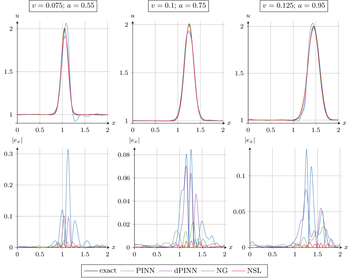
Figure 1 displays the results of the four approaches, for four distinct values of the variance . Note that each value of the variance corresponds to a new problem to solve, with a new neural network to train. The truly parametric case is treated in the following section. For dPINN, we take (corresponding to time steps) for , and (corresponding to time steps) otherwise. For NG and NSL, we take (corresponding to time steps). We have chosen epochs for the inner optimization problems (3.3) of the NSL method, since the problem converged quickly and more epochs did not bring noticeable improvements.
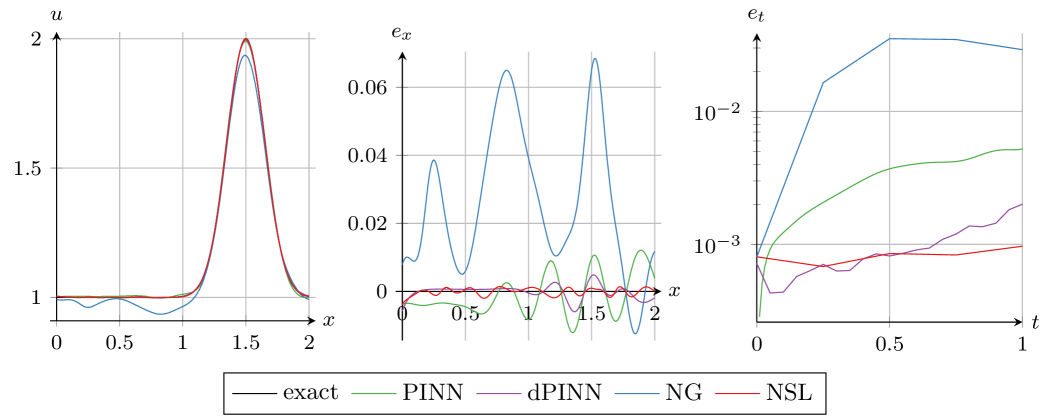
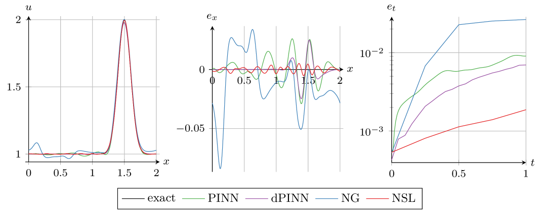
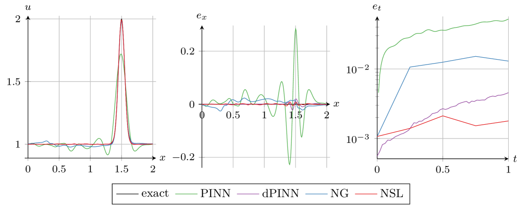
We observe that the NSL method outperforms the other methods, by almost an order of magnitude in some cases. Indeed, the NSL method is able to capture both the peak of the Gaussian pulse and the constant state far away from the peak, with good accuracy.
On the contrary, the other methods tend to either diffuse the peak or create oscillations in the constant state, or both. Notably, the dPINN method required quite a restrictive time step to perform well; larger time steps led to numerical instabilities and oscillations destroying the simulation quality. Moreover, it also required better solving the optimization problems, which led to an increased number of epochs during the initialization phase and the inner epochs, compared to the NG and NSL methods. Therefore, even if the results of the dPINN method are quite good, they come at a large computational cost, at least times as large as the NG and NSL methods.
To better understand the role of , we display in Figure 2 the results of the methods for and for several values of . Namely, we show the error as a function of time, for , which corresponds to , , , , , and time steps, respectively. For time steps , we perform epochs for the inner optimization problems instead of , to help convergence. The results of the dPINN method are only shown for , since otherwise it does not converge.
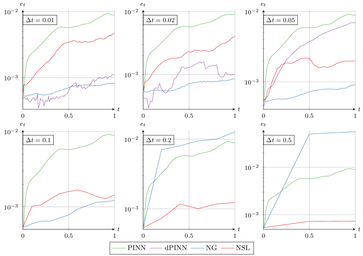
On the one hand, for both the NG and dPINN methods, we observe that the accuracy is improved when using smaller time steps, overtaking the PINN for . On the other hand, interestingly, we note that smaller time steps do not necessarily lead to better results for the NSL method, at least in this simpler case. We expect this observation to change when considering time-dependent advection coefficients, or advection-diffusion equations.
4.1.2 Parametric case
We now turn to the parametric version of (4.1), where this time the variance and the advection coefficient are both parameters. The hyperparameters are defined in Table 9. Compared to the previous case, the PINN is now solving a 4D problem (1D in space, 1D in time, and 2D in the parameter space), and the dPINN, NG and NSL neural networks are solving 3D problems (1D in space and 2D in the parameter space). This makes the problem quite a bit more complex, which explains the increased number of epochs, collocation points and neurons in the hidden layers.
An added difficulty for the dPINN, NG and NSL methods is that the initial condition does not depend on , so the network has to learn to ignore the second parameter for learning the initial condition, but to use it for the time evolution. To overcome that difficulty, on the one hand, we set a rather small time step for NG and dPINN (). On the other hand, the NSL time step is still large (), but the number of epochs in the inner optimization problems has been increased to . With this setup, on the one hand, for NG and NSL, it takes seconds to train the network approximating the initial condition, while the whole time stepping takes about minute (meaning that NSL iterations are about times slower than NG ones). On the other hand, it takes about minutes to train the PINN. The dPINN method is much slower than the other ones: indeed, training and solving the optimization problems totals about minutes. This is due to the larger dimension of the problem, requiring additional collocation points.
As a first test, we take three values of the parameters , and we draw the solutions (top panels) and associated errors (bottom panels) in Figure 3. We observe that NSL consistently yields a better approximation than the other methods; namely, it is less oscillatory.
To get a more quantitative estimation of the error with respect to the parameter set , we compute the norm of (computed at the final time) for randomly sampled parameters in . The results are presented in Table 1, where we report the minimum, average and maximum of the norm of over , as well as its standard deviation. We observe that, over the whole parameter set , the NSL method consistently gives very good results. On average, the NSL results are quite close to the PINN. However, this comes at a much lower computational cost, as the NSL method is about times faster than the PINN method.
| PINN | dPINN | NG | NSL | |
|---|---|---|---|---|
| min | ||||
| avg | ||||
| max | ||||
| std |
4.2 Nonconstant advection in 2D
We now provide some numerical experiments on advection equations with nonconstant advection coefficients, in two and three space dimensions, and with several parameters. The first test case consists in a 2D advection equation with a rotating transport, presented in Section 4.2.1. The second one, presented in Section 4.2.2 is a 2D advection equation, without parameters, mimicking the Vlasov equation representing the movement of charged particles in an electric field.
In this section, we do not consider the dPINN method any longer, since it is not competitive with NSL and NG for the problems at hand, especially in terms of stability condition, and to simplify the presentation.
4.2.1 2D parametric rotating transport
We first consider a 2D advection equation with a nonconstant advection coefficient, leading to a rotating advection equation within the unit disk . The advection equation reads
with the divergence-free advection vector field given by
| (4.2) |
The parametric exact solution is given by
where and , and with the parameters , where is in the parameter set . Equipped with the exact solution, the initial condition is then simply given by .
Note that the advection field (4.2) is no longer constant in space, although it still leads to an exact solution to the ODE (2.4) governing the characteristic curves. This exact solution is given by
where we have set
This allows us to apply the second branch of Algorithm 1 when computing the characteristic curves in the NSL method.
The hyperparameters are given in Table 10. We note that, for this experiment, more collocation points are used to approximate the integrals. Indeed, the solution is a Gaussian function, highly localized in both parameter space and physical space, which requires a better Monte-Carlo approximation.
We run the PINN, NG and NSL methods on this problem. On the one hand, we set a fixed time step for the NG method, leading to time steps and for the NSL method, leading to time steps. With this setup, it takes about seconds to train the network approximating the initial condition, and about seconds to run both the NG and the NSL methods. On the other hand, since the PINN is now solving a 5D problem, a larger network has to be used, leading to a training time of about minutes.
The results are displayed on Figure 4, where we show the approximate solutions (top panels) and the associated errors (bottom panels). We observe a very good agreement of the NSL solution, especially close to the peak of the Gaussian bump, which is much better approximated with the NSL method than with the other methods.
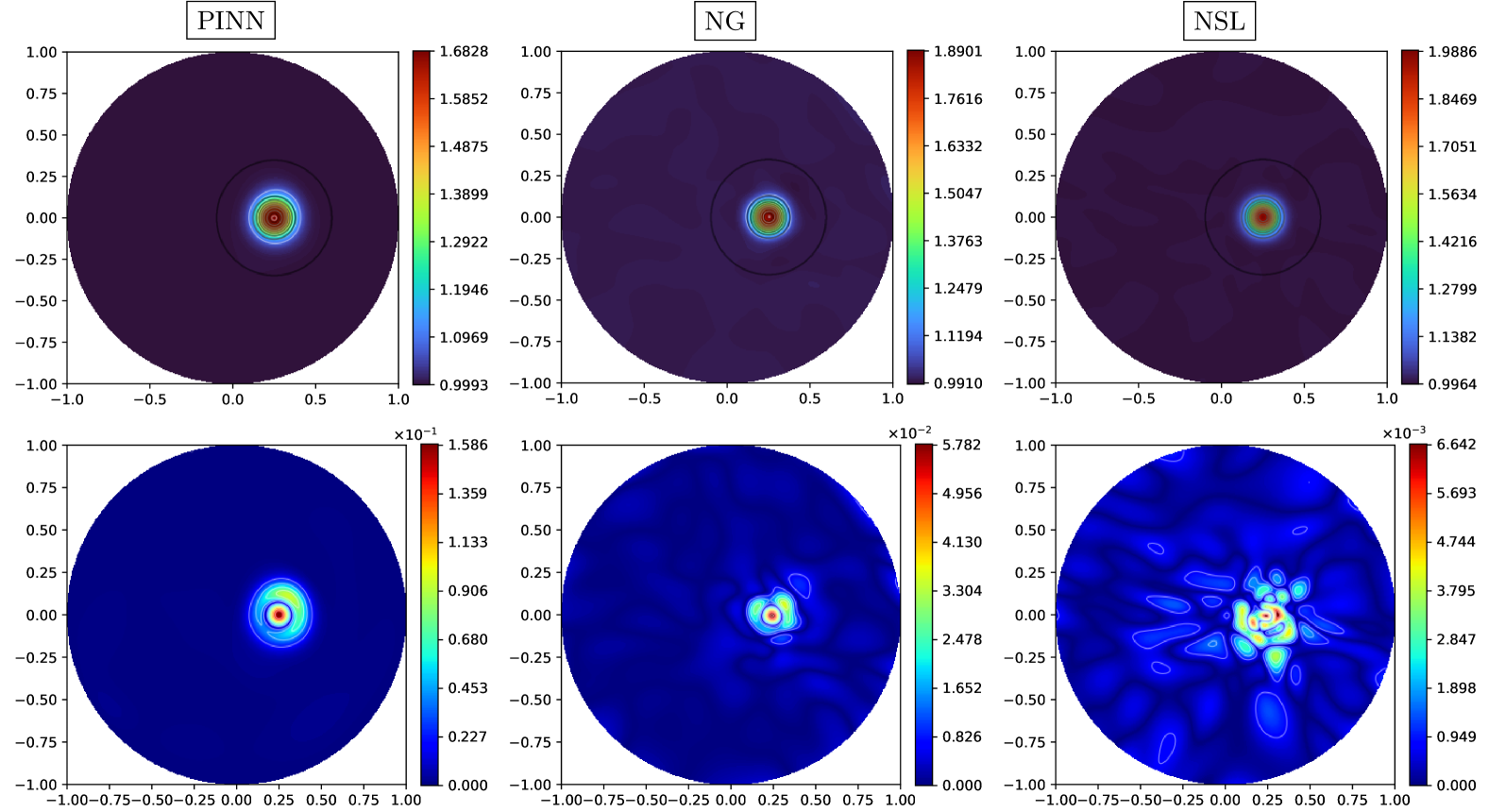
For a refined comparison of the methods, we run the three methods on randomly sampled parameters in , and report the statistics on the errors in Table 2. In both and norms, we observe a significant gain in accuracy for the NG and NSL methods over the PINN. Furthermore, the NSL method outperforms the NG method, by a factor of in norm, and up to in norm.
| NSL | NG | PINN | ||||
|---|---|---|---|---|---|---|
| error | error | error | error | error | error | |
| min | ||||||
| avg | ||||||
| max | ||||||
| std | ||||||
4.2.2 1D1V Vlasov equation
The next test case in this series is a Vlasov equation in one space dimension and one velocity dimension. It is nothing but a 2D advection equation without parameters, whose setup is described in e.g. [4]. It is given by the following set of equations, with periodic boundary conditions in and :
| (4.3) |
with the initial condition
This time, neither the advection equation (4.3) nor the characteristic ODE (2.4) have a closed-form solution. To obtain a reference solution, we numerically solve (4.3) using a classical semi-Lagrangian scheme333The semi-Lagrangian code is inspired from the one developed by Pierre Navaro, available at https://pnavaro.github.io/python-notebooks/19-LandauDamping.html. on a Cartesian grid, with in space and in velocity, and with time steps per second (leading to e.g. time steps for ). Moreover, to solve the characteristic ODE, we use the third branch of Algorithm 1, with sub-time-steps.
Since this problem is more complex than the previous ones, in that it leads to a sheared solution with filaments, we ran the simulation in double precision. Moreover, the hyperparameters are adjusted accordingly. Namely, more collocation points are used to approximate the integrals. All hyperparameters are given in Table 11. We elect to use a fixed time step for the NG method, corresponding to time iterations, and for the NSL method, corresponding to time iterations. This leads to a computation time of about minutes for the PINN, minute for the NSL method and minutes for the NG method (plus seconds for the initial condition). The results are displayed in Figures 5, 6 and 7.
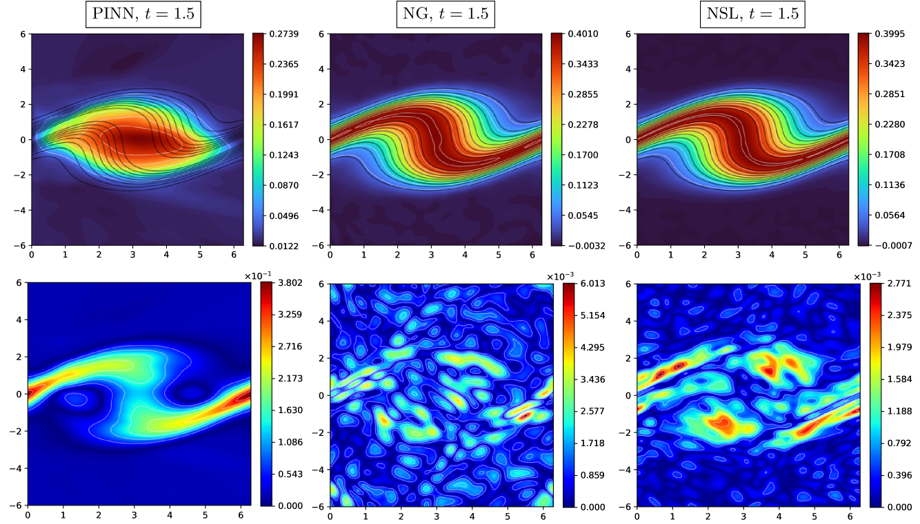

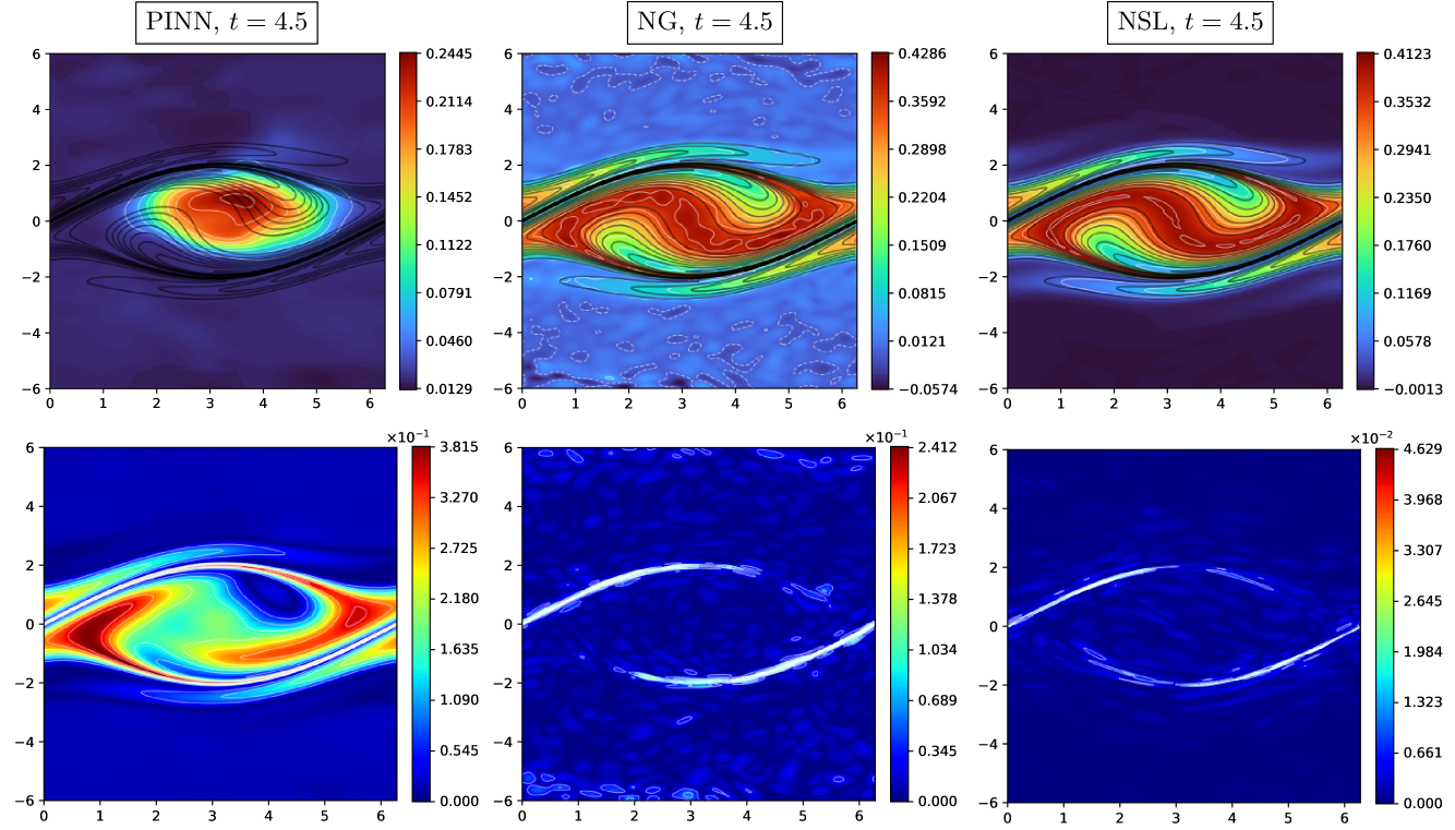
This experiment shows the limits of the PINN when approximating a solution with fine structures. Indeed, the results of the PINN (displayed in the left panels of the figures) are quite poor, and the solution is diffused away. Since the PINN learns all times at once, there is no reason why the early times should be better approximated than the later times, and this is confirmed by observing the results.
The NG scheme, on the other hand, provides a better approximation of the solution than the PINN. However, even though the solution is less diffusive, it remains more oscillatory, especially close to the filaments. In particular, we see that the solution becomes negative in some regions, which is not physical.
Finally, the NSL method provides the best approximation among the three tested methods. Namely, the fine filaments present in the solution are well-captured, although the approximation quality decreases with time since the filamentation process increases. This decrease in quality is not improved when decreasing the time step, even locally in time (e.g. taking two time steps between and ). This motivates the next section, where we will introduce preconditioning and other techniques to further improve the accuracy and efficiency of our method.
| time | PINN error | NG error | NSL error | |||
|---|---|---|---|---|---|---|
| error | error | error | error | error | error | |
Lastly, we report in Table 3 the and errors of each method, bearing in mind that the error may not be very informative in this case, since we are comparing solutions with sharp gradients. These errors confirm our observations from Figures 5, 6 and 7, namely that PINN is the least accurate method, while NSL is the most accurate one, improving the error by a factor of about and the error by a factor of about compared to the NG method, all for a third of the computational cost.
4.3 Transport equation in a cylinder
From this section onwards, we will only consider the NSL method, and check it on several benchmark problems. The present section is devoted to testing the improvements proposed in Section 3.5. To that end, we consider an advection equation in three space dimensions and two parameter dimensions. The space domain is a cylinder . The solution is governed by the advection equation
supplemented with periodic boundary conditions in the third variable, and a suitable initial condition. Namely, we set the advection field to
| (4.4) |
corresponding to a rotation in the first two variables and a constant advection in the third one. Moreover, the (parameter-dependent) exact solution is a bump function, which reads
where we have set
where denotes the modulo operation. The two parameters and respectively represent the position of the center of the Gaussian bump, and its variance. The exact solution corresponds to a rotation of the bump around the -axis, with a constant advection in the direction. We take a time step , corresponding to time steps.
We compare the results of the NSL method, as described before, to the improved version equipped with natural gradient preconditioning (Section 3.5.1) and adaptive sampling (Section 3.5.2). The adaptive sampling is based on the zeroes of the gradient of the approximate solution, i.e.,
in Algorithm 3, where is a safety factor to avoid division by zero. Furthermore, we take , and in Algorithm 3. We test three configurations for the improved NSL method: first with a small network (configuration (a)), then with a larger network but few epochs (configuration (b)), and lastly with a larger network, as well as additional epochs and collocation points (configuration (c)). The hyperparameters are summarized in Table 4, for each configuration.
| Hyperparameter | NSL | improved NSL | ||
|---|---|---|---|---|
| configuration (a) | configuration (b) | configuration (c) | ||
| (init.) | ||||
| (iter.) | ||||
To report the results, we perform a parametric study over randomly sampled parameters in , and report the statistics in Table 5, along with the computation time. The first configuration of the improved NSL method decreases the computation time by a factor of roughly , and decreases the average error by a factor of in norm, in norm. These substantial increases in accuracy and efficiency make the improved NSL method even more competitive with other neural methods. We remark that the network is really quite small, and natural gradient preconditioning shows that solving the optimization problem is an important bottleneck in the training of the neural network. Moving on to larger networks and additional epochs, we observe a further decrease of the error, alongside a (substantial) increase in the computation time. We observe that, in configuration (b), the increase in epochs in not sufficient to improve the accuracy and solve the optimization problems more efficiently than in configuration (a). However, in configuration (c), the further increase in both epochs and collocation points allows us to further decrease the error by a factor of around . The downside is that the computation time is increased by a factor of about . All in all, we see that the improved NSL method is able to provide a very accurate solution for a small computational cost, and that this accuracy can be improved further should one be willing to pay the computation time.
| min | avg | max | std | ||
| non-improved | error | ||||
| error | |||||
| computation time (init.) | \qty121.78 | ||||
| computation time (iter.) | \qty296.58 | ||||
| configuration (a) | error | ||||
| error | |||||
| computation time (init.) | \qty19.06 | ||||
| computation time (iter.) | \qty26.35 | ||||
| configuration (b) | error | ||||
| error | |||||
| computation time (init.) | \qty110.20 | ||||
| computation time (iter.) | \qty149.87 | ||||
| configuration (c) | error | ||||
| error | |||||
| computation time (init.) | \qty774.73 | ||||
| computation time (iter.) | \qty1267.12 | ||||
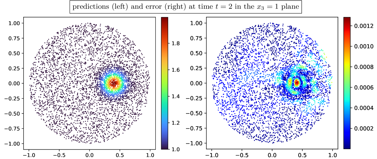
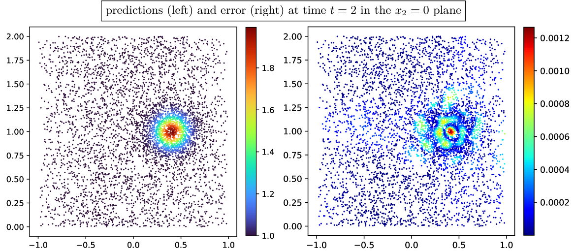
To give an idea of the adaptively sampled points, we represent in Figures 8 and 9 the predictions (left panels) and associated errors (right panels) of the improved method, in configuration (c), at the final time , for the physical parameters and , and in two planes where the Gaussian bump is localized ( for Figure 8 and for Figure 9). We have displayed adaptively sampled points out of the collocation points actually used in this test case. In both cases, in addition to noticing that the errors produced by the improved NSL method are quite low, we observe that the adaptively sampled points are concentrated around the peak of the Gaussian bump, where the solution is the most challenging to approximate, and where the error is the largest, even though the adaptive sampling procedure is not aware of the exact solution.
Remark 3.
For the remainder of the numerical experiments, we elect to use hyperparameters similar to configuration (c). This leads to higher computation times, but better accuracy for the optimization problems. Using hyperparameters similar to configuration (a) would lead to significantly lower computation times, at the cost of a decrease in accuracy.
4.4 Deformation of level-set functions
Equipped with the improved version of NSL, we now test it on two challenging test cases, namely the deformation of level-set functions, in 2D (Section 4.4.1) and 3D (Section 4.4.2). These test cases, described in e.g. [39, 10], consist in the transport of a level-set function by a time-dependent advection field. They are particularly interesting since, while the transient solution is not known, the final solution is the initial condition itself, which allows for a better assessment of the accuracy of the method. Since we are approximating a level-set function, we use in Algorithm 3; we take , and .
4.4.1 Deformation of a 2D level-set function
The initial condition of this two-dimensional level-set advection test case is, accordingly, a level-set function. It represents the disk of radius centered at , i.e.,
The shape then undergoes a deformation, according to the following time-dependent advection field:
where is the final time. The shape is most deformed at time , and goes back to the initial shape at time . The hyperparameters for this experiment are given in Table 12. We take a time step , corresponding to time steps. Note that additional time steps are performed compared to previous experiments; this is to obtain a good discretization of the time-dependent advection field. With this configuration, the full computation takes about one hour.
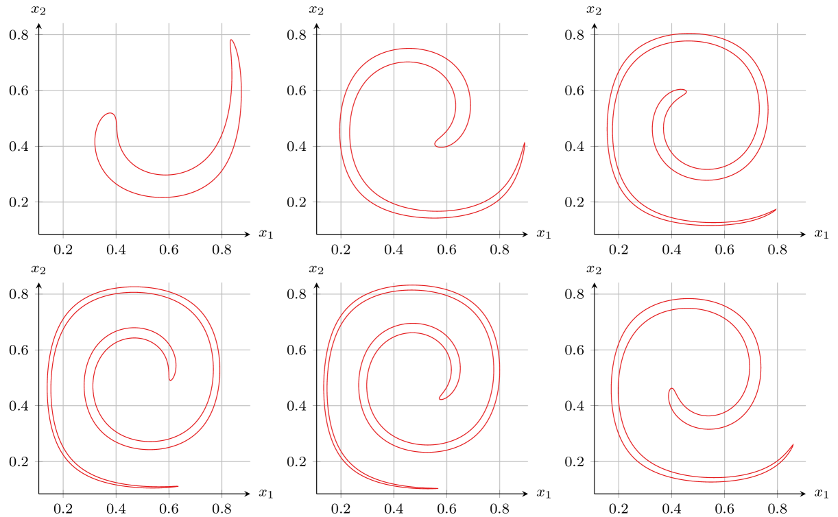
Figure 10 depicts the zero contour of the approximate level-set function at several times. We observe a good agreement with the reference solution from [39, 10]. Namely, the deformation of the shape is well-captured, even at its most deformed, for .
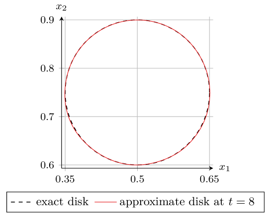
To get a better view of the accuracy of the NSL method, we compare the NSL solution at to the exact solution, which is nothing but the initial condition. Namely, the zero contour of the exact solution is the disk of radius centered at . This comparison is carried out in Figure 11, where we observe a very good agreement between the two solutions, further validating the accuracy of the NSL method.
4.4.2 Deformation of a 3D level-set function
After the 2D level-set deformation, we move on to a more complex three-dimensional test case. This time, the initial condition is a level-set function of the sphere of radius centered at , given by
It is then advected with the time-dependent advection field
Similarly to Section 4.4.1, we recover the initial condition for . We take a time step , which corresponds to time steps. This leads, together with the hyperparameters reported in Table 12, lead to a computation time of about minutes. Same as the 2D level-set deformation, additional points are sampled around the zeroes of the approximate solution.
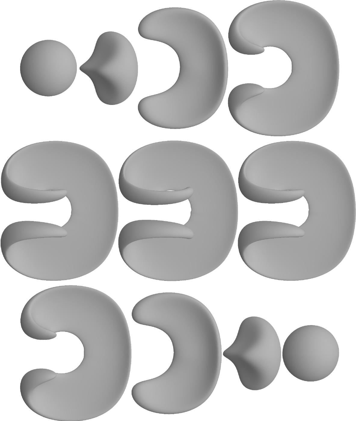
First, in Figure 12, we display the zero contour of the approximate level-set function at all computed times between and , with a step of . The approximate zero contour is well-captured by the NSL scheme, as can be seen by comparing it to the reference solution from [39, 10].
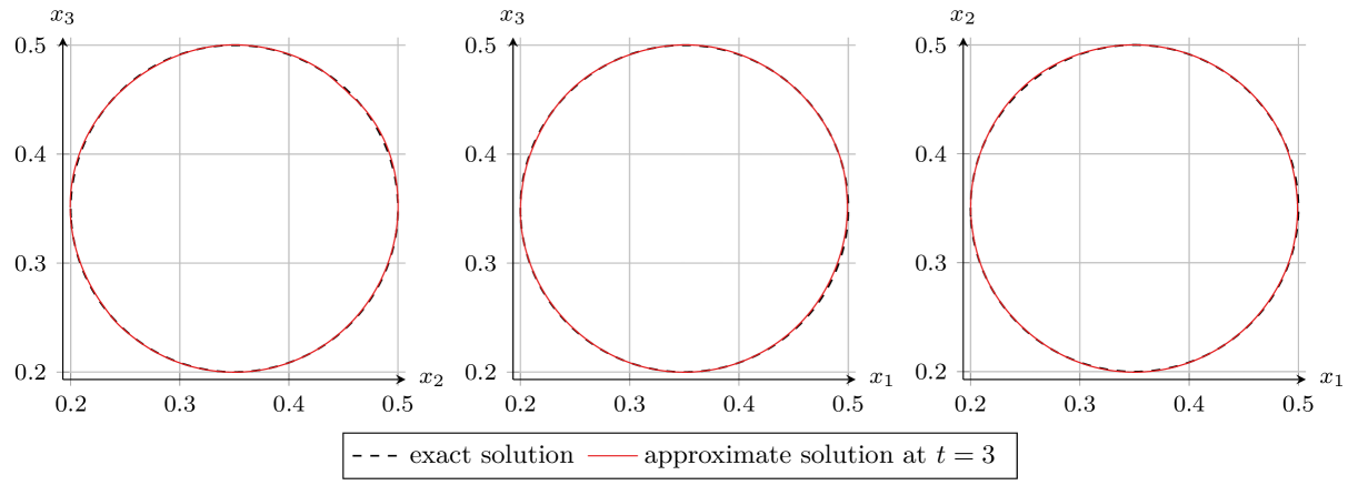
Second, Figure 13 shows the zero contour of the approximate level-set function, comparing it to the exact solution . To do so, we display the 3D sphere sliced by the planes , and , leading to three 2D graphs. Once again, we observe a very good agreement between the NSL solution and the exact solution, even for this more complex three-dimensional problem.
4.5 High-dimensional advection-diffusion equations
This last section is dedicated to the approximation of advection-diffusion equations, following Section 3.4. In a -dimensional space domain , we define a constant advection field and a constant diffusion coefficient . The advection-diffusion equation (1.1) then reads
We first check the convergence of the scheme in Section 4.5.1, and then we test it on two high-dimensional problems: a periodic solution in Section 4.5.2 and a Gaussian solution in Section 4.5.3.
4.5.1 Convergence study
For this study, the space domain is supplemented with periodic boundary conditions. We define the exact solution, for all and , by
where for all is used to make the problem harder by introducing a different phase shift in each dimension. In practice, the diffusion coefficient is set to . For this experiment, natural gradient preconditioning is used, but not adaptive sampling, since there are no obvious areas in which additional points should be sampled. Moreover, activation functions are employed.
To test the convergence of the scheme as decreases, we select dimension to avoid unnecessary computational costs but still have a reasonably high-dimensional problem. According to Remark 3, we choose to use hyperparameters corresponding to a higher accuracy, at the cost of computation time. This leads us to taking layers, epochs for the initialization, epochs per time step, and collocation points. We take the final time , and we vary by running the scheme with several numbers of time steps. This study is done in To that end, we compute the following and relative errors:
for a set of collocation points uniformly drawn in . Note that the true error would have required a multiplication by the volume of the domain, which is . The errors are reported in Figure 14, where we observe, as expected, that the error decreases with order as the number of time steps increases. Moreover, the scheme is indeed stable for all time steps, even very large ones.
| 4 | ||
|---|---|---|
| 8 | ||
| 16 | ||
| 32 | ||
| 64 | ||
| 128 |
4.5.2 High-dimensional periodic solution
Then, we check the error and the computation time with respect to the dimension , making sure that they do not explode with the dimension. We still consider the periodic solution from Section 4.5.1. We fix the dimension-dependent final time
which corresponds to the time at which the diffusion halves the amplitude of the solution. The interval is discretized into time steps.
Compared to the previous case, we still use activation functions, but the number of layers depends on the dimension : namely, we take . Moreover, we use Fourier features to enhance the solution approximation, see [59], with Fourier features. The other hyperparameters are the same with respect to the dimension: the number of collocation points is , the number of epochs is for the initialization and for each iteration.
| dimension | computation time | relative error | ||
|---|---|---|---|---|
| init. | iter. | |||
| 1 | \qty50.12 | \qty13.81 | ||
| 2 | \qty55.96 | \qty17.07 | ||
| 3 | \qty76.06 | \qty25.12 | ||
| 4 | \qty121.85 | \qty36.62 | ||
| 5 | \qty198.20 | \qty57.18 | ||
| 6 | \qty341.12 | \qty101.95 | ||
| 7 | \qty591.64 | \qty168.27 | ||
| 8 | \qty1000.97 | \qty262.36 | ||
The results are reported in Table 6. We note that the computation time does not increase exponentially with the dimension. We observe that the error remains roughly constant with the dimension, hovering around in norm and in norm.
4.5.3 High-dimensional Gaussian solution
We now consider a more localized, non-separable solution. Namely, in a non-periodic domain, the exact solution is given by
where the mean is defined by and the covariance satisfies , with the identity matrix in dimension . The symmetric positive-definite initial covariance satisfies
and we take the diffusion coefficient . This solution corresponds to a nonsymmetric Gaussian pulse being advected and diffused along the diagonal of the domain. To have a good representation of this solution, we take the space domain , and the final time is . This corresponds, at the final time, to the solution being diffused by a factor of around .
This time, we use both the natural gradient preconditioning and the adaptive sampling. For the latter, we sample using the gradient of the solution, like in (4.4), and we set , and . Regarding the other hyperparameters, we take time steps, activation functions, and the number of layers is . The number of epochs is for the initialization and for each iteration (except for where ), and we take collocation points.
| dimension | computation time | relative error | ||
|---|---|---|---|---|
| init. | iter. | |||
| 1 | \qty33.67 | \qty49.08 | ||
| 2 | \qty39.29 | \qty41.85 | ||
| 3 | \qty46.32 | \qty51.41 | ||
| 4 | \qty58.18 | \qty66.80 | ||
| 5 | \qty78.26 | \qty89.54 | ||
| 6 | \qty106.11 | \qty122.03 | ||
| 7 | \qty146.83 | \qty168.42 | ||
| 8 | \qty217.95 | \qty243.31 | ||
The results are reported in Table 7. Similarly to the previous case, the computation time does not increase exponentially, and the errors remain at roughly the same level. The errors tend to decrease with the dimension, which is expected since the solution becomes more localized as the dimension grows.
5 Conclusion
In this work, we have introduced a neural version of the well-known semi-Lagrangian method. This method has the advantage of being able to solve advection-diffusion in high dimensions, without any time step requirements for stability. It is based on modelling the approximate solution using a neural network, and then using nonlinear optimization to solve the resulting backwards transport equation. Numerical results show the performance of the method, especially compared to (albeit more general) methods from the literature. Namely, we show that a good accuracy is retained in high dimensions, for a comparatively low computational cost.
To improve Vlasov simulations, the next step consists in exploring improved network architectures, e.g. using Fourier features [59], PirateNets [60], or Kolmogorov-Arnold Networks (KAN, see [42]). Domain decomposition and parallelism will also be employed to optimize computational efficiency, in the spirit of e.g. [19]. We will also propose a better adaptive sampling, to further reduce the computational cost, especially at high dimensions. Work like [43] could be adapted. Our neural strategy will also be extended to solving the Vlasov-Poisson [36], Vlasov-Maxwell [41], and gyrokinetic [24] models, going towards high-dimensional applications in plasma physics.
Acknowledgments
This work was supported by the French National Research Agency through projects ANR-23-PEIA-0004 (PDE-AI, all three authors), ANR-22-EXNU-0002 (Exa-MA, all three authors), ANR-21-CE46-0014 (Milk, E. F. and L. N.), and ANR-22-CE25-0017 (OptiTrust, V. M.-D.).
References
- [1] S. Amari and S. C. Douglas. Why natural gradient? In Proceedings of the 1998 IEEE International Conference on Acoustics, Speech and Signal Processing, ICASSP ’98 (Cat. No.98CH36181), volume 2 of ICASSP-98, pages 1213–1216. IEEE, 1998.
- [2] J. Ansel and E. Yang et al. PyTorch 2: Faster Machine Learning Through Dynamic Python Bytecode Transformation and Graph Compilation. In Proceedings of the 29th ASPLOS, Volume 2, volume 5 of ASPLOS ’24, pages 929–947. ACM, 2024.
- [3] A. Beltran-Pulido, I. Bilionis, and D. Aliprantis. Physics-Informed Neural Networks for Solving Parametric Magnetostatic Problems. IEEE Trans. Energy Convers., 37(4):2678–2689, 2022.
- [4] J. Berman and B. Peherstorfer. Randomized Sparse Neural Galerkin Schemes for Solving Evolution Equations with Deep Networks. In Thirty-seventh Conference on Neural Information Processing Systems, 2023.
- [5] V. Biesek and P. H. de Almeida Konzen. Burgers’ PINNs with implicit Euler Transfer Learning. Rev. Mundi Eng., Tecnol. Gest., 9(4), 2024.
- [6] O. Bokanowski and G. Simarmata. Semi-Lagrangian discontinuous Galerkin schemes for some first- and second-order partial differential equations. ESAIM: M2AN, 50(6):1699–1730, 2016.
- [7] L. Bonaventura, E. Calzola, E. Carlini, and R. Ferretti. Second Order Fully Semi-Lagrangian Discretizations of Advection-Diffusion-Reaction Systems. J. Sci. Comput., 88(1), 2021.
- [8] L. Bonaventura, R. Ferretti, and L. Rocchi. A fully semi-Lagrangian discretization for the 2D incompressible Navier-Stokes equations in the vorticity-streamfunction formulation. Appl. Math. Comput., 323:132–144, 2018.
- [9] J. Bruna, B. Peherstorfer, and E. Vanden-Eijnden. Neural Galerkin schemes with active learning for high-dimensional evolution equations. J. Comput. Phys., 496:112588, 2024.
- [10] C. Bui, C. Dapogny, and P. Frey. An accurate anisotropic adaptation method for solving the level set advection equation. Int. J. Numer. Meth. Fl., 70(7):899–922, 2011.
- [11] F. Charles, B. Després, and M. Mehrenberger. Enhanced Convergence Estimates for Semi-Lagrangian Schemes Application to the Vlasov–Poisson Equation. SIAM J. Numer. Anal., 51(2):840–863, 2013.
- [12] Y. Chen, W. Guo, and X. Zhong. A learned conservative semi-Lagrangian finite volume scheme for transport simulations. J. Comput. Phys., 490:112329, 2023.
- [13] Y. Chen, W. Guo, and X. Zhong. Conservative semi-lagrangian finite difference scheme for transport simulations using graph neural networks. J. Comput. Phys., 526:113768, 2025.
- [14] A. Cohen and G. Migliorati. Optimal weighted least-squares methods. SMAI J. Comput. Math., 3:181–203, 2017.
- [15] N. Crouseilles, M. Mehrenberger, and É. Sonnendrücker. Conservative semi-Lagrangian schemes for Vlasov equations. J. Comput. Phys., 229(6):1927–1953, 2010.
- [16] N. Crouseilles, M. Mehrenberger, and F. Vecil. Discontinuous Galerkin semi-Lagrangian method for Vlasov-Poisson. ESAIM: Proceedings, 32:211–230, 2011.
- [17] N. Crouseilles, T. Respaud, and É. Sonnendrücker. A forward semi-Lagrangian method for the numerical solution of the Vlasov equation. Comput. Phys. Commun., 180(10):1730–1745, 2009.
- [18] T. De Ryck and S. Mishra. Error analysis for physics-informed neural networks (PINNs) approximating Kolmogorov PDEs. Adv. Comput. Math., 48(6), 2022.
- [19] V. Dolean, A. Heinlein, S. Mishra, and B. Moseley. Multilevel domain decomposition-based architectures for physics-informed neural networks. Comput. Method. Appl. M., 429:117116, 2024.
- [20] J. Douglas, Jr and T. F. Russell. Numerical methods for convection-dominated diffusion problems based on combining the method of characteristics with finite element or finite difference procedures. SIAM J. Numer. Anal., 19(5):871–885, 1982.
- [21] W. E and B. Yu. The Deep Ritz Method: A Deep Learning-Based Numerical Algorithm for Solving Variational Problems. Commun. Math. Stat., 6(1):1–12, 2018.
- [22] L. Einkemmer and I. Joseph. A mass, momentum, and energy conservative dynamical low-rank scheme for the vlasov equation. J. Comput. Phys., 443:110495, 2021.
- [23] L. Einkemmer, K. Kormann, J. Kusch, R. G. McClarren, and J.-M. Qiu. A review of low-rank methods for time-dependent kinetic simulations, 2024. Preprint.
- [24] V. Grandgirard et al. A 5D gyrokinetic full- global semi-Lagrangian code for flux-driven ion turbulence simulations. Comput. Phys. Commun., 207:35–68, 2016.
- [25] M. Falcone and R. Ferretti. Convergence analysis for a class of high-order semi-Lagrangian advection schemes. SIAM J. Numer. Anal., 35(3):909–940, 1998.
- [26] R. Ferretti. A Technique for High-Order Treatment of Diffusion Terms in Semi-Lagrangian Schemes . Commun. Comput. Phys., 8(2):445–470, 2010.
- [27] R. Ferretti and M. Mehrenberger. Stability of semi-Lagrangian schemes of arbitrary odd degree under constant and variable advection speed. Math. Comput., 89(324):1783–1805, 2020.
- [28] F. Filbet, É. Sonnendrücker, and P. Bertrand. Conservative Numerical Schemes for the Vlasov Equation. J. Comput. Phys., 172(1):166–187, 2001.
- [29] M. A. Finzi, A. Potapczynski, M. Choptuik, and A. G. Wilson. A Stable and Scalable Method for Solving Initial Value PDEs with Neural Networks. In The Eleventh International Conference on Learning Representations, 2023.
- [30] A. Hamiaz, M. Mehrenberger, H. Sellama, and É. Sonnendrücker. The semi-Lagrangian method on curvilinear grids. Commun. Appl. Ind. Math., 7(3):99–137, 2016.
- [31] Q. Hong, J. W. Siegel, Q. Tan, and J. Xu. On the Activation Function Dependence of the Spectral Bias of Neural Networks. preprint, 2022.
- [32] Z. Hu, K. Shukla, G. E. Karniadakis, and K. Kawaguchi. Tackling the curse of dimensionality with physics-informed neural networks. Neural Networks, 176:106369, 2024.
- [33] S. Jin, Z. Ma, and K. Wu. Asymptotic-Preserving Neural Networks for Multiscale Time-Dependent Linear Transport Equations. J. Sci. Comput., 94(3), 2023.
- [34] M. Kast and J. S. Hesthaven. Positional embeddings for solving PDEs with evolutional deep neural networks. J. Comput. Phys., 508:112986, 2024.
- [35] K. Kormann. A Semi-Lagrangian Vlasov Solver in Tensor Train Format. SIAM J. Sci. Comput., 37(4):B613–B632, 2015.
- [36] K. Kormann, K. Reuter, and M. Rampp. A massively parallel semi-Lagrangian solver for the six-dimensional Vlasov-Poisson equation. Int. J. High Perform. C., 33(5):924–947, 2019.
- [37] A. Krishnapriyan, A. Gholami, S. Zhe, R. Kirby, and M. W. Mahoney. Characterizing possible failure modes in physics-informed neural networks. In Thirty-fourth Conference on Neural Information Processing Systems, 2021.
- [38] L. Á. Larios-Cárdenas and F. Gibou. Error-correcting neural networks for semi-Lagrangian advection in the level-set method. J. Comput. Phys., 471:111623, 2022.
- [39] R. J. LeVeque. High-Resolution Conservative Algorithms for Advection in Incompressible Flow. SIAM J. Numer. Anal., 33(2):627–665, 1996.
- [40] L. Li and C. Yang. APFOS-Net: Asymptotic preserving scheme for anisotropic elliptic equations with deep neural network. J. Comput. Phys., 453:110958, 2022.
- [41] H. Liu, X. Cai, G. Lapenta, and Y. Cao. Conservative semi-Lagrangian kinetic scheme coupled with implicit finite element field solver for multidimensional Vlasov Maxwell system. Commun. Nonlinear Sci., 102:105941, 2021.
- [42] Z. Liu and Y. Wang et al. KAN: Kolmogorov-Arnold Networks. In The Thirteenth International Conference on Learning Representations, 2025.
- [43] Z. Mao and X. Meng. Physics-informed neural networks with residual/gradient-based adaptive sampling methods for solving partial differential equations with sharp solutions. Appl. Math. Mech., 44(7):1069–1084, 2023.
- [44] X. Meng, Z. Li, D. Zhang, and G. E. Karniadakis. PPINN: Parareal physics-informed neural network for time-dependent PDEs. Comput. Method. Appl. M., 370:113250, 2020.
- [45] S. Mishra and R. Molinaro. Physics informed neural networks for simulating radiative transfer. J. Quant. Spectrosc. Radiat. Transfer, 270:107705, 2021.
- [46] J. Müller and M. Zeinhofer. Achieving high accuracy with PINNs via energy natural gradient descent. In A. Krause, E. Brunskill, K. Cho, B. Engelhardt, S. Sabato, and J. Scarlett, editors, Proceedings of the 40th International Conference on Machine Learning, volume 202 of Proceedings of Machine Learning Research, pages 25471–25485. PMLR, 23–29 Jul 2023.
- [47] L. Nurbekyan, W. Lei, and Y. Yang. Efficient Natural Gradient Descent Methods for Large-Scale PDE-Based Optimization Problems. SIAM J. Sci. Comput., 45(4):A1621–A1655, 2023.
- [48] O. Pironneau. On the transport-diffusion algorithm and its applications to the Navier-Stokes equations. Numer. Math., 38:309–332, 1982.
- [49] J.-M. Qiu and C.-W. Shu. Positivity preserving semi-Lagrangian discontinuous Galerkin formulation: theoretical analysis and application to the Vlasov–Poisson system. J. Comput. Phys., 230(23):8386–8409, 2011.
- [50] A. Quarteroni and A. Valli. Numerical approximation of partial differential equations, volume 23. Springer Science & Business Media, 2008.
- [51] M. Raissi, P. Perdikaris, and G. E. Karniadakis. Physics-informed neural networks: A deep learning framework for solving forward and inverse problems involving nonlinear partial differential equations. J. Comput. Phys., 378:686–707, 2019.
- [52] M. Restelli, L. Bonaventura, and R. Sacco. A semi-Lagrangian discontinuous Galerkin method for scalar advection by incompressible flows. J. Comput. Phys., 216(1):195–215, 2006.
- [53] J. A. Rossmanith and D. C. Seal. A positivity-preserving high-order semi-Lagrangian discontinuous Galerkin scheme for the Vlasov–Poisson equations. J. Comput. Phys., 230(16):6203–6232, 2011.
- [54] N. Schwencke and C. Furtlehner. ANaGRAM: A natural gradient relative to adapted model for efficient PINNs learning. In The Thirteenth International Conference on Learning Representations, 2025.
- [55] É. Sonnendrücker, J. Roche, P. Bertrand, and A. Ghizzo. The Semi-Lagrangian Method for the Numerical Resolution of the Vlasov Equation. J. Comput. Phys., 149(2):201–220, 1999.
- [56] A. Staniforth and J. Côté. Semi-Lagrangian Integration Schemes for Atmospheric Models—A Review. Mon. Weather Rev., 119(9):2206–2223, 1991.
- [57] J. Stiasny and S. Chatzivasileiadis. Physics-informed neural networks for time-domain simulations: Accuracy, computational cost, and flexibility. Electr. Pow. Syst. Res., 224:109748, 2023.
- [58] N. Sukumar and A. Srivastava. Exact imposition of boundary conditions with distance functions in physics-informed deep neural networks. Comput. Method. Appl. M., 389:114333, 2022.
- [59] M. Tancik, P. Srinivasan, B. Mildenhall, S. Fridovich-Keil, N. Raghavan, U. Singhal, R. Ramamoorthi, J. Barron, and R. Ng. Fourier Features Let Networks Learn High Frequency Functions in Low Dimensional Domains. In H. Larochelle, M. Ranzato, R. Hadsell, M. F. Balcan, and H. Lin, editors, Advances in Neural Information Processing Systems, volume 33, pages 7537–7547. Curran Associates, Inc., 2020.
- [60] S. Wang, B. Li, Y. Chen, and P. Perdikaris. PirateNets: Physics-informed Deep Learning with Residual Adaptive Networks. J. Mach. Learn. Res., 25:1–51, 2024.
- [61] S. Wang, S. Sankaran, and P. Perdikaris. Respecting causality for training physics-informed neural networks. Comput. Method. Appl. M., 421:116813, 2024.
- [62] C. Wu, M. Zhu, Q. Tan, Y. Kartha, and L. Lu. A comprehensive study of non-adaptive and residual-based adaptive sampling for physics-informed neural networks. Comput. Methods Appl. Mech. Engrg., 403:115671, 2023.
- [63] D. Xiu and G. E. Karniadakis. A Semi-Lagrangian High-Order Method for Navier-Stokes Equations. J. Comput. Phys., 172(2):658–684, 2001.
- [64] C. Yang and M. Mehrenberger. Highly accurate monotonicity-preserving Semi-Lagrangian scheme for Vlasov-Poisson simulations. J. Comput. Phys., 446:110632, 2021.
- [65] B. Zhang, G. Cai, H. Weng, W. Wang, L. Liu, and B. He. Physics-informed neural networks for solving forward and inverse Vlasov-Poisson equation via fully kinetic simulation. Mach. Learn.: Sci. Technol., 4(4):045015, 2023.
- [66] N. Zheng, D. Hayes, A. Christlieb, and J.-M. Qiu. A Semi-Lagrangian Adaptive-Rank (SLAR) Method for Linear Advection and Nonlinear Vlasov-Poisson System. J. Comput. Phys., page 113970, 2025.
Appendix A Hyperparameters for the numerical experiments
This section regroups all the hyperparameters used in the numerical experiments. We denote by:
-
•
the number of collocation points, i.e., the number of points uniformly sampled to discretize the space domain and approximate the integrals in the optimization problems, see Algorithm 2;
-
•
the number of epochs;
-
•
the activation function;
-
•
(resp. ) the boundary (resp. initial) loss function coefficient, i.e., the coefficient by which the boundary (resp. initial) loss function is multiplied when weakly imposing the boundary (resp. initial) conditions in the PINN;
-
•
(resp. ) the number of collocation points in the boundary (resp. initial) integrals in the PINN;
-
•
the list of layer sizes,
-
•
the learning rate (note that no learning rate is reported when natural gradient preconditioning is deployed).
Note that or being set to means that the corresponding loss function is not used, and that the boundary or initial conditions are strongly imposed. Moreover, the activation function corresponds to the following regularized hat function, see [31]:
For each experiment, we report the hyperparameters used:
-
•
to train the PINN;
-
•
to compute the initial dofs for the dPINN, NG and NSL methods (in the column called “initialization”);
-
•
to iterate the dPINN method, i.e., to solve the nonlinear optimization problem (2.8) at each time step;
-
•
to iterate the NSL method, i.e., to solve the nonlinear optimization problem (3.3) at each time step.
| Hyperparameter | PINN | initialization | dPINN iterations | NSL iterations |
|---|---|---|---|---|
| N/A | N/A | |||
| N/A | N/A | |||
| N/A | N/A | N/A | ||
| N/A | N/A | N/A | ||
| N/A | N/A | N/A | ||
| N/A | N/A | N/A |
| Hyperparameter | PINN | initialization | dPINN iterations | NSL iterations |
|---|---|---|---|---|
| N/A | N/A | |||
| N/A | N/A | |||
| N/A | N/A | N/A | ||
| N/A | N/A | N/A | ||
| N/A | N/A | N/A | ||
| N/A | N/A | N/A |
| Hyperparameter | PINN | NG and SL initialization | NSL iterations |
|---|---|---|---|
| N/A | |||
| N/A | |||
| N/A | N/A | ||
| N/A | N/A | ||
| N/A | N/A | ||
| N/A | N/A |
| Hyperparameter | PINN | NG and SL initialization | NSL iterations |
|---|---|---|---|
| N/A | |||
| N/A | |||
| N/A | N/A | ||
| N/A | N/A | ||
| N/A | N/A | ||
| N/A | N/A |
| Hyperparameter | Section 4.4.1 | Section 4.4.2 |
|---|---|---|